TTP03-11

QCD corrections to single top quark production
in electron photon interactions
J.H. Kühn, C. Sturm, and P. Uwer

Institut für Theoretische Teilchenphysik, Universität Karlsruhe
76128 Karlsruhe, Germany

Abstract

Single top quark production in electron photon interactions provides a clean environment for the measurement of the Cabbibo-Kobayashi-Maskawa matrix element $V_{tb}$. Aiming an experimental precision at the percent level the knowledge of radiative corrections is important. In this paper we present results for the radiative corrections in quantum chromodynamics.

1 Introduction

One of the fundamental unsolved problems of todays high-energy physics is the exact mechanism of electroweak symmetry breaking (EWSB). Due to the fact that only the top quark couples with a Yukawa coupling of order one to the so far unobserved Higgs boson it is natural to assume that the top quark plays a special rôle in the context of the EWSB. For example in so-called dynamical symmetry breaking models the scalar Higgs field — responsible for the spontaneous symmetry breaking in the Standard Model — is replaced by a composite scalar operator. Such an operator could be built for example from heavy fermion fields. Having eliminated the elementary scalar field from the theory the problem of the large mass corrections due to quantum corrections is solved. Examples for such models are technicolour models (for a review see ref. [1] and references therein), top-condensate models [2], and top-colour models [3, 4]. For the search of such extensions a precise understanding of the top quark sector of the standard model is necessary.

At hadron colliders both single top quark production as well as top quark pair production have been studied extensively in the past. The differential cross section for top quark pair production is known to next-to-leading order (NLO) accuracy in quantum chromodynamics (QCD) [5, 6, 7, 8]. In addition the resummation of logarithmic enhanced contributions has been studied in detail in refs. [9, 10, 11, 12, 13]. Recently also the spin correlations between top quark and anti-top quark were calculated at NLO in QCD [14]. Due to the fact that single top quark production provides an excellent opportunity to test the charged-current weak-interaction of the top quark it has also attracted a lot of interest in the past. In particular NLO corrections were studied in refs. [15, 16, 17, 18]. In ref. [18] the NLO corrections for the fully differential cross section is given keeping also the spin information of the top quark. On the experimental side the situation is not very conclusive for the moment as far as single top quark production is concerned. Due to limited statistics at run I of the Tevatron collider only upper bounds were obained in ref. [19]. In ref. [20] the possibility to measure the electroweak couplings in single top quark production at the LHC is studied. In particular also the sensitivity to new physics is discussed.

As far as lepton colliders are concerned much effort has been devoted to top quark pair production in $e^{+}e^{-}$-annihilation. In particular the total cross section in the threshold region is known at next-to-next-leading order (NNLO) in QCD. (For an overview of the theoretical status we refer to ref. [21].) Momentum [22, 23] as well as angular [24, 25] distributions were studied in detail. In the continuum region the total cross section for massive quarks is known to order ${\alpha_{s}}^{2}$ in the coupling constant of the strong interaction [26]. In order ${\alpha_{s}}^{3}$ the quartic mass corrections to the total cross section are also known [27]. Also less inclusive observables have been studied in great detail. For example the spin structure of top anti-top system is completely known at order ${\alpha_{s}}$ [28, 29, 30, 31, 32] and partially known at order ${\alpha_{s}}^{2}$ [33]. Futhermore the 3-jet results obtained for massive $b$-quarks [34, 35, 36, 37, 38, 39] are also applicable to top quark physics [40].

Less attention has been devoted to single top quark production. Studies at tree level can be found for example in refs. [41, 42, 43, 44, 45]. In the refs. [41, 42] special emphasis was put on single top quark production at LEP II. For a top quark mass arround 175 GeV the production rates in the standard model are to small to be detectable at LEP II. This was recently confirmed by the L3 collaboration [46]. In ref. [45] also the single top quark production in electron photon collisions is studied. The electron photon reaction provides a clean environment for the study of single top quark production because there is no background from top quark pair production. As a consequence this reaction is very well suited for the measurement of the weak couplings of the top quark. In particular it has been shown in ref. [45] that using polarised beams the Cabibbo-Kobayashi-Maskawa (CKM) matrix element $V_{tb}$ can be measured with an uncertainty of 1% at the 2$\sigma$ level. In this analysis $10^{4}$ top quark events were assumed which corresponds to a luminosity of 100 fb^-1 of an electron photon collider operating at $\sqrt{s}=500$ GeV.
Aiming an accuracy at the percent level it is clear that the knowledge of the QCD corrections is mandatory. This is the main purpose of the present paper. In addition we study the structure of logarithmic enhanced contributions which are related to initial state singularities. The full dependence on the $b$-quark mass is kept. This allows a systematic comparison between the structure function approach and the fixed-order calculation. Furthermore close to the threshold effects of the finite $b$-quark mass are important. To calculate the QCD corrections we use the effective W-approximation. In the $W$-approximation the scattering process which needs to be studied is $W^{+}\gamma\to t\bar{b}$. Using the $W$-approximation which describes the momentum distribution of the $W$-boson in the electron a prediction for $e^{+}\gamma\to t\bar{b}\nu_{e}$ can be obtained. A more detailed discussion is given in section 5.

The outline of the paper is as follows. In section 2 we discuss the kinematics and the leading order results for the reaction $W^{+}\gamma\to t\bar{b}$. The virtual corrections to this process are discussed in section 3. In section 4 the real corrections are calculated. In particular the cancellation of the infrared singularities is shown. In the following section we present the results for the subreaction $W^{+}\gamma\to t\bar{b}$ as well as for the reaction $e^{+}\gamma\to t\bar{b}\bar{\nu}_{e}$. We finally close with our conclusions in section 6.

2 Kinematics and leading-order results

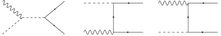
Figure 2.1: Feynman diagrams for $W^{+}\gamma\to t\bar{b}$ in leading-order

In the following we study the reaction

$$W^{+}({k_{w}})+\gamma({k_{\gamma}})\to t({k_{t}})+\bar{b}({k_{b}}),$$ (2.1)

where we treat both outgoing quarks as massive. For later use it is convenient to define dimensionless variables. In particular we define the rescaled masses

$$z_{i}={m_{i}^{2}\over s}$$ (2.2)

and the energy fractions

$$x_{i}={2(k\cdot k_{i})\over s}$$ (2.3)

with $k={k_{w}}+{k_{\gamma}}$ and $s=k^{2}$. For the reaction given in eq. (2.1) the energy fractions are fixed completely by the kinematics:

$${x_{t}}=1+{z_{t}}-{z_{b}},\quad\mbox{and}\quad{x_{b}}=1+{z_{b}}-{z_{t}}.$$ (2.4)

This is no longer true when the emission of an additional gluon is considered (c.f. section 4 ). The calculation of the Born matrix elements for the reaction (2.1) is straightforward so we just quote the results here. The corresponding Feynman diagrams are shown in fig. 2.1. For the $W$ boson we distinguish between longitudinal and transverse polarization while for the photon we average over the incoming polarization. For partons in the final state the polarization (and the colour) is summed over. In terms of the leading-order squared matrix elements $|{\cal M}_{0}^{T,L}|^{2}$ for transversely/longitudinally polarized $W$-bosons the differential cross sections are given by

$${d\sigma^{T,L}\over d\Omega}={N\*\lambda_{bt}\over 64\*\pi^{2}\*(1-{z_{w}})\*s}\*{1\over{\cal N}_{\,T,L}}\*\sum_{{\mbox{{\mbox{\scriptsize$\gamma,t,b$ Pol.}}}}}|{\cal M}_{0}^{T,L}|^{2},$$ (2.5)

where $\lambda_{bt}$ is defined as

$$\lambda_{bt}=\lambda(1,{z_{b}},{z_{t}})$$ (2.6)

with

$$\lambda(x,y,z)=\sqrt{x^{2}+y^{2}+z^{2}-2\*x\*y-2\*x\*z-2\*y\*z}.$$ (2.7)

The number of colours is denoted by $N$. For transversely polarized $W$-bosons the normalization ${\cal N}_{T}$ is given by ${\cal N}_{T}=2\cdot 2$. For longitudinally polarized $W$-bosons we have ${\cal N}_{L}=2$. The squared matrix element for longitudinally polarized $W$-bosons is given by

$$\sum_{{\mbox{{\mbox{\scriptsize$\gamma,t,b$ Pol.}}}}}|{\cal M}_{0}^{L}|^{2} = {2\*\kappa\over 9\*{z_{w}}\*(1-{z_{w}})^{2}}\*\Bigg{(}{8\*({z_{b}}^{3}-2\*{z_{b}}^{2}\*{z_{t}}+{z_{b}}\*{z_{t}}^{2}+(3\*{z_{b}}^{2}-{z_{b}}\*{z_{t}})\*{z_{w}})\over\left({x_{b}}-\lambda_{bt}\*{z}\right)^{2}}$$ (2.8)

$$+ {32\*({z_{b}}^{2}\*{z_{t}}-2\*{z_{b}}\*{z_{t}}^{2}+{z_{t}}^{3}+(3\*{z_{t}}^{2}-{z_{b}}\*{z_{t}})\*{z_{w}})\over\left({x_{t}}+\lambda_{bt}\*{z}\right)^{2}}+{l_{1}^{L}\over{x_{b}}-\lambda_{bt}\*{z}}+{l_{2}^{L}\over{x_{t}}+\lambda_{bt}\*{z}}$$

$$+ 12\*{z}\*\lambda_{bt}\*(3\*{z_{b}}-3\*{z_{t}}-{z_{w}})\*{z_{w}}+18\*{z}^{2}\*\lambda_{bt}^{2}\*{z_{w}}^{2}+18\*{z_{b}}^{2}-9\*{z_{b}}\*(1+4\*{z_{t}})-9\*{z_{t}}$$

$$+ 18\*{z_{t}}^{2}+{z_{w}}\*(36\*{z_{b}}^{2}+12\*{z_{b}}\*(1-6\*{z_{t}})+60\*{z_{t}}+36\*{z_{t}}^{2})$$

$$+ {z_{w}}^{2}\*(2-18\*{z_{b}}^{2}+39\*{z_{t}}-18\*{z_{t}}^{2}+3\*{z_{b}}\*(5+12\*{z_{t}}))\Bigg{)},$$

where ${z}$ denotes the cosine of the scattering angle

$${z}=\cos\theta_{b\gamma}=-\cos\theta_{t\gamma}$$ (2.9)

in the center of mass system and the prefactor $\kappa$ is given by

$$\kappa=8\*\sqrt{2}\*\pi\alpha\*{G_{f}}\*{|V_{tb}|^{2}}\*{z_{w}}\*s.$$ (2.10)

Here ${G_{f}}$ denotes the Fermi constant and $V_{tb}$ the Cabbibo-Kobayashi-Maskawa (CKM) matrix element. The functions $l_{1}^{L},\,l_{2}^{L}$ are given by

$$l_{1}^{L} = 2\*(-10\*{z_{b}}^{3}-2\*{z_{b}}^{2}\*(1-11\*{z_{t}})+{z_{b}}\*(1+4\*{z_{t}}-14\*{z_{t}}^{2})+{z_{t}}-2\*{z_{t}}^{2}+2\*{z_{t}}^{3}$$ (2.11)

$$-2\*{z_{w}}\*(19\*{z_{b}}^{2}+{z_{t}}^{2}+4\*{z_{b}}\*(1-3\*{z_{t}}))+{z_{w}}^{2}\*({z_{t}}-7\*{z_{b}})),$$

$$l_{2}^{L} = 8\*({z_{b}}-2\*{z_{b}}^{2}+2\*{z_{b}}^{3}+(1+4\*{z_{b}}-8\*{z_{b}}^{2})\*{z_{t}}-2\*(1-5\*{z_{b}})\*{z_{t}}^{2}-4\*{z_{t}}^{3}$$ (2.12)

$$+{z_{w}}\*(-2\*{z_{b}}^{2}-2\*(4-9\*{z_{b}})\*{z_{t}}-20\*{z_{t}}^{2})+{z_{w}}^{2}\*({z_{b}}-7\*{z_{t}})).$$

The above matrix element is given in 4 dimension. In the context of the QCD corrections we will also need the squared matrix elements in $d$ dimensions. The matrix element in $d=4-2{\epsilon}$ dimensions for longitudinally polarized $W$-bosons is given by

$$\sum_{{\mbox{{\mbox{\scriptsize$\gamma,t,b$ Pol.}}}}}|{\cal M}_{0,d}^{L}|^{2}=\sum_{{\mbox{{\mbox{\scriptsize$\gamma,t,b$ Pol.}}}}}|{\cal M}_{0}^{L}|^{2}+{\epsilon}\*\kappa\*{2\*({z_{b}}+{z_{t}})\over{z_{w}}}\*\left[1-{1\over 9}\*\left({2\over{x_{b}}-\lambda_{bt}\*{z}}+{8\over{x_{t}}+\lambda_{bt}\*{z}}\right)\right].$$ (2.13)

In the derivation of the results above we used

$${\epsilon}_{L}^{\mu}({k_{w}}){\epsilon}_{L}^{\nu}({k_{w}})^{\ast}=\left({{k_{w}}^{\mu}{k_{w}}^{\nu}\over{m_{w}}^{2}}-{{k_{w}}^{\mu}{k_{\gamma}}^{\nu}+{k_{w}}^{\nu}{k_{\gamma}}^{\mu}\over({k_{w}}\cdot{k_{\gamma}})}+{{m_{w}}^{2}{k_{\gamma}}^{\mu}{k_{\gamma}}^{\nu}\over({k_{w}}\cdot{k_{\gamma}})^{2}}\right)$$ (2.14)

with ${\epsilon}_{L}({k_{w}})$ being the polarization vector of the incoming longitudinally polarized $W$ boson. The squared matrix element for transversely polarized $W$-bosons reads:

$$\sum_{{\mbox{{\mbox{\scriptsize$\gamma,t,b$ Pol.}}}}}|{\cal M}_{0}^{T}|^{2} = {2\*\kappa\over 9\*{z_{w}}\*(1-{z_{w}})^{2}}\*\Bigg{(}{64\*{z_{t}}\*{z_{w}}\*({z_{b}}-{z_{t}}-{z_{w}})\over\left({x_{t}}+\lambda_{bt}\*{z}\right)^{2}}-{16\*{z_{b}}\*{z_{w}}\*({z_{b}}-{z_{t}}+{z_{w}})\over\left({x_{b}}-\lambda_{bt}\*{z}\right)^{2}}$$ (2.15)

$$+ {l_{1}^{T}\over{x_{b}}-\lambda_{bt}\*{z}}+{l_{2}^{T}\over{x_{t}}+\lambda_{bt}\*{z}}+6\*{z}\*\lambda_{bt}\*\bigg{(}{z_{w}}\*(1-3\*{z_{b}}+3\*{z_{t}})+6\*{z_{w}}^{2}\*({z_{t}}-{z_{b}})$$

$$+ {z_{w}}^{3}\*(1+3\*{z_{b}}-3\*{z_{t}})\bigg{)}-9\*{z}^{2}\*\lambda_{bt}^{2}\*{z_{w}}\*(1+{z_{w}}^{2})+{z_{w}}\*(-19-45\*{z_{b}}^{2}-18\*{z_{t}}$$

$$- 45\*{z_{t}}^{2}+{z_{b}}\*(18+90\*{z_{t}}))+{z_{w}}^{2}\*(36\*{z_{b}}^{2}-{z_{b}}\*(12+72\*{z_{t}})-60\*{z_{t}}+36\*{z_{t}}^{2})$$

$$+ {z_{w}}^{3}\*(-19-9\*{z_{b}}^{2}+6\*{z_{t}}-9\*{z_{t}}^{2}-{z_{b}}\*(6-18\*{z_{t}}))\Bigg{)}$$

with

$$l_{1}^{T} = 4\*{z_{w}}\*\left(1+14\*{z_{b}}^{2}+2\*{z_{b}}\*(1-8\*{z_{t}})-2\*{z_{t}}+2\*{z_{t}}^{2}+2\*{z_{w}}\*(7\*{z_{b}}-{z_{t}})+{z_{w}}^{2}\right),$$ (2.16)

$$l_{2}^{T} = 16\*{z_{w}}\*\left(1+2\*{z_{b}}^{2}-{z_{b}}\*(2+10\*{z_{t}})+2\*{z_{t}}+8\*{z_{t}}^{2}-2\*{z_{w}}\*({z_{b}}-4\*{z_{t}})+{z_{w}}^{2}\right),$$ (2.17)

where we have used

$$\sum{\epsilon}_{T}^{\mu}({k_{w}}){\epsilon}_{T}^{\nu}({k_{w}})^{\ast}=\left(-g^{\mu\nu}+{{k_{w}}^{\mu}{k_{\gamma}}^{\nu}+{k_{w}}^{\nu}{k_{\gamma}}^{\mu}\over({k_{w}}\cdot{k_{\gamma}})}-{{m_{w}}^{2}{k_{\gamma}}^{\mu}{k_{\gamma}}^{\nu}\over({k_{w}}\cdot{k_{\gamma}})^{2}}\right)$$ (2.18)

for the sum over the two different transverse polarizations of the $W$-boson.

For later use we also give the squared matrix element for transversely polarized $W$-bosons in $d$ dimensions:

$$\sum_{{\mbox{{\mbox{\scriptsize$\gamma,t,b$ Pol.}}}}}|{\cal M}^{T}_{\rm d}|^{2}=\sum_{{\mbox{{\mbox{\scriptsize$\gamma,t,b$ Pol.}}}}}|{\cal M}^{T}|^{2}+{\epsilon}\*\kappa\*\Bigg{[}2\*{z}^{2}\*\lambda_{bt}^{2}-{4\over 3}\*{z}\*\lambda_{bt}\*(1+3\*({z_{b}}-zt))$$ (2.19)

$$- {1\over 9\*(1-{z_{w}})^{2}}\*\Bigg{(}{32\*{z_{b}}\*({z_{b}}+{z_{t}}-{z_{w}})\over({x_{b}}-\lambda_{bt}\*{z})^{2}}+{128\*{z_{t}}\*({z_{b}}+{z_{t}}-{z_{w}})\over({x_{t}}+\lambda_{bt}\*{z})^{2}}$$

$$+ {16\over{x_{b}}-\lambda_{bt}\*{z}}\*\left(1-{z_{b}}-5\*{z_{b}}^{2}-(1+4\*{z_{b}})\*{z_{t}}+{z_{t}}^{2}-(1-5\*{z_{b}}+{z_{t}})\*{z_{w}}+{z_{w}}^{2}\right)$$

$$+ {64\over{x_{t}}+\lambda_{bt}\*{z}}\*\left(1-{z_{b}}+{z_{b}}^{2}-(1+{z_{b}})\*{z_{t}}-2\*{z_{t}}^{2}-(1+{z_{b}}-2\*{z_{t}})\*{z_{w}}+{z_{w}}^{2}\right)$$

$$- 2\*\left(-36\*({z_{b}}+{z_{t}})+37\*(1+{z_{w}}^{2})-38\*{z_{w}}+3\*(1-{z_{w}})^{2}\*(2+3\*({z_{b}}-{z_{t}}))\*({z_{b}}-{z_{t}})\right)\Bigg{)}\Bigg{]}$$

$$- 4\*\kappa\*{\epsilon}^{2}\*\left[1-{1\over 9}\*\left({2\over{x_{b}}-\lambda_{bt}\*{z}}+{8\over{x_{t}}+\lambda_{bt}\*{z}}\right)\right]$$

Performing the remaining integration over the scattering angle we obtain the leading-order total cross section $\sigma_{\rm tot}^{T,L}$ for transversely/longitudinally polarized $W$-bosons:

$$\sigma_{\rm tot}^{T,L}={1\over 9\*\sqrt{2}}\*{\alpha\*{G_{f}}\*{|V_{tb}|^{2}}\*N\over(1-{z_{w}})^{3}}\*{1\over{\cal N}_{\,T,L}}\*\left(l_{1}^{T,L}\*\ln\left({1+\beta_{b}\over 1-\beta_{b}}\right)+l_{2}^{T,L}\*\ln\left({1+\beta_{t}\over 1-\beta_{t}}\right)+K^{T,L}\right),$$ (2.20)

with

$$K^{L} = 2\*\lambda_{bt}\*\Big{(}28\*{z_{b}}^{2}-9\*{z_{t}}+28\*{z_{t}}^{2}-{z_{b}}\*(9+56\*{z_{t}})+2\*{z_{w}}\*(18\*{z_{b}}^{2}+41\*{z_{t}}+18\*{z_{t}}^{2}$$ (2.21)

$$+{z_{b}}\*(5-36\*{z_{t}}))-{z_{w}}^{2}\*(-8+12\*{z_{b}}^{2}-3\*{z_{b}}\*(1+8\*{z_{t}})-27\*{z_{t}}+12\*{z_{t}}^{2})\Big{)}$$

$$K^{T} = 4\*{z_{w}}\*\lambda_{bt}\*\Big{(}-24\*{z_{b}}^{2}+6\*{z_{b}}\*(3+8\*{z_{t}})-11-12\*{z_{t}}-24\*{z_{t}}^{2}-2\*{z_{w}}\*(-9\*{z_{b}}^{2}+3\*{z_{b}}\*(1+6\*{z_{t}})$$ (2.22)

$$+5+15\*{z_{t}}-9\*{z_{t}}^{2})-{z_{w}}^{2}\*(6\*{z_{b}}^{2}-12\*{z_{b}}\*{z_{t}}+11-6\*{z_{t}}+6\*{z_{t}}^{2})\Big{)}.$$

The velocities $\beta_{t},\beta_{b}$ of the outgoing quarks in the center-of-mass system are given by

$$\beta_{t}={\lambda_{bt}\over 1+{z_{t}}-{z_{b}}},\quad\mbox{and}\quad\beta_{b}={\lambda_{bt}\over 1+{z_{b}}-{z_{t}}}.$$ (2.23)

Note that the relation between the cross sections for unpolarized, transversely and longitudinally polarized $W$-bosons is given by

$$\sigma={1\over 3}(2\sigma^{T}+\sigma^{L}).$$ (2.24)

Furthermore we note that the structure of the logarithmic terms in eq. (2.20) is universal and can be obtained without an explicit calculation. In particular the singular contribution in the limit ${m_{b}}\to 0$ can be written as

$$\sigma(W^{+}({k_{w}})\gamma({k_{\gamma}})\to t({k_{t}})\bar{b}({k_{b}}))\stackrel{{\scriptstyle m_{b}\to 0}}{{\longrightarrow}}\int_{0}^{1}dx\;f_{b/\gamma}(x,{m_{b}}^{2},s)\times\sigma(W^{+}({k_{w}})b(x{k_{\gamma}})\to t({k_{t}})),$$ (2.25)

where $f_{b/\gamma}(x,{m_{b}}^{2},s)$ can be interpreted as the bottom distribution in the photon (at scale $s$):

$$f_{b/\gamma}(x,{m_{b}}^{2},s)={\alpha\over 2\pi}Q_{b}^{2}P_{\gamma\to q\bar{q}}(x)\ln\left({s\over{m_{b}}^{2}}\right)$$ (2.26)

with the Altarelli-Parisi $P_{\gamma\to q\bar{q}}(x)$ kernel [47] given by

$$P_{\gamma\to q\bar{q}}(x)=x^{2}+(1-x)^{2}.$$ (2.27)

(We denote with $Q_{b}$ the electric charge of the $b$-quark in units of the elementary charge $e$.) A more detailed discussion will be given in section 5 where the so-called structure function approach is investigated.

3 Virtual corrections

In this section we discuss the calculation of the virtual corrections. In particular we sketch briefly a few technicalities of the calculation, discuss the ultraviolet (UV) and infrared singularities (IR), and carry out the renormalization.

We work in renormalized perturbation theory, which means that the bare quantities (fields and couplings) are expressed in terms of renormalized quantities. By this procedure one obtains two contributions: one is the original Lagrangian but now in terms of the renormalized quantities, the second contribution are the so-called counter terms:

$${\cal L}(\Psi_{0},A_{0},m_{0},g_{0})={\cal L}(\Psi_{R},A_{R},m_{R},g_{R})+{\cal L}_{ct}(\Psi_{R},A_{R},m_{R},g_{R}).$$ (3.1)

The first contribution yields the same Feynman rules as the bare Lagrangian but with the bare quantities replaced by renormalized ones. In the following we renormalize the quark field and the quark mass in the on-shell scheme. The conversion of the on-shell mass to the frequently used $\overline{\mbox{MS}}$ mass or to any other renormalization scheme can be performed at the end of the calculation. In spite of the fact that the calculation presented here is a one-loop calculation, it is still leading-order in the strong coupling constant ${\alpha_{s}}$. As a consequence the renormalization of the coupling constant does not appear.

Whereas in the $\overline{\mbox{MS}}$ scheme the renormalization constants contain only UV singularities, in the on-shell scheme they contain also infrared divergences. We use dimensional regularization to treat both types of divergencies. Although at the very end all the divergences must cancel it is worthwhile to distinguish between UV and IR singularities so that one can check the UV finiteness after renormalization and the cancellation of the IR singularities independently.

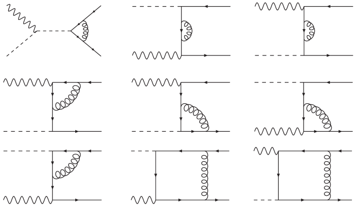
Figure 3.1: Virtual corrections to $W^{+}\gamma\to t\bar{b}$

To start with let us discuss the contribution of the one-loop diagrams before renormalization, that is the contribution from ${\cal L}(\Psi_{R},\ldots,m_{R},g_{R})$. The corresponding Feynman diagrams are shown in fig. 3.1. The calculation of the one-loop amplitude is tedious but straightforward. To reduce the one-loop tensor integrals to scalar one-loop integrals we used the Passarino-Veltman reduction procedure [48]. The two one-loop box integrals are given by

$$D_{0,1}^{d} = {1\over i\pi^{2}}\int d^{d}\ell{1\over(\ell^{2}-{m_{t}}^{2})(\ell-{k_{t}})^{2}((\ell-{k_{t}}-{k_{b}})^{2}-{m_{b}}^{2})((\ell-{k_{t}}-{k_{b}}+{k_{\gamma}})^{2}-{m_{b}}^{2})},$$

$$D_{0,2}^{d} = \left.D_{0,1}^{d}\right|_{({m_{t}},{k_{t}})\leftrightarrow({m_{b}},{k_{b}})}.$$ (3.2)

All the simpler topologies follow from these integrals by dropping one, two or three propagators. For example, using the standard notation [48] the infrared divergent triangle integral is given by

$$C^{d}_{0}(1,2,3)={1\over i\pi^{2}}\int d^{d}\ell{1\over(\ell^{2}-{m_{t}}^{2})(\ell-{k_{t}})^{2}((\ell-{k_{t}}-{k_{b}})^{2}-{m_{b}}^{2})}.$$ (3.3)

The one-point, two-point and the finite three-point integrals have been calculated in the standard way using Feynman parameterization. We have checked that our results for these integrals agree with the numerical evaluation given by the FF package of G. J. van Oldenborgh [49, 50]. Here we give only explicit results for the two IR divergent integrals. The triangle integral is given by

$$(2\pi\mu)^{2{\epsilon}}\,\,{\rm Re}C^{d}_{0}(1,2,3) = {1\over s\*\lambda_{bt}}\*\Gamma(1+{\epsilon})\left({4\pi\mu^{2}\over s}\right)^{\epsilon}\*\bigg{[}{1\over{\epsilon}}\*\ln(\rho)-{2\over 3}\*\pi^{2}-2\*\ln(\lambda_{bt})\*\ln(\rho)$$ (3.4)

$$- {1\over 4}\*(\ln({\omega_{t}})^{2}+\ln({\omega_{b}})^{2})-{{\rm Li}_{2}}({\omega_{b}})-{{\rm Li}_{2}}({\omega_{t}})\bigg{]}+O({\epsilon})$$

$$= {1\over s\*\lambda_{bt}}\*\Gamma(1+{\epsilon})\left({4\pi\mu^{2}\over s}\right)^{\epsilon}{1\over{\epsilon}}\*\ln(\rho)+\overline{C}_{0}(1,2,3),$$

with

$$\omega_{i}={1-\beta_{i}\over 1+\beta_{i}}\quad(i=t,b),$$ (3.5)

and

$$\rho=\sqrt{{1-{z_{t}}-{z_{b}}-\lambda_{bt}\over 1-{z_{t}}-{z_{b}}+\lambda_{bt}}}.$$ (3.6)

To calculate the infrared divergent box integral we have used two different methods. First we have considered a subtracted version of the integral which can be calculated in 4 dimensions using Feynman parameterization. From this result the desired result for the box integral can be easily obtained. The second method is based on the result given in ref. [51]. There the infrared singularity is regulated by a small photon mass $\lambda$. This result can be converted to dimensional regularization using the substitution [52]

$$\ln(\lambda^{2})\to{1\over{\epsilon}}-\gamma+\ln(4\pi\mu^{2}).$$ (3.7)

We found agreement of the results obtained by the two methods. The final expression reads

$$(2\pi\mu)^{2{\epsilon}}{\rm Re}D^{d}_{0,1}=\*{1\over s^{2}\lambda_{tb}}{2\over(1-{z_{w}})\*({x_{b}}-{z}\lambda_{bt})}\*\Gamma(1+{\epsilon})\left({4\pi\mu^{2}\over s}\right)^{\epsilon}$$

$$\times\bigg{\{}-{1\over{\epsilon}}\ln(\rho)+\ln(\rho)\*\ln\left({{({x_{b}}-{z}\*\lambda_{bt})^{2}\*\lambda_{bt}^{2}\over 4\*{z_{b}}}}\right)-\ln({x_{3}})^{2}$$

$$+2\*\ln\left({{x_{3}}+\rho\over 1+\rho\*{x_{3}}}\right)\*\ln({x_{3}})-2\*{{\rm Li}_{2}}(-\rho\*{x_{3}})+{{\rm Li}_{2}}(\rho^{2})-2\*{{\rm Li}_{2}}(-\rho/{x_{3}})+{1\over 2}\*\pi^{2}\bigg{\}},$$ (3.8)

with

$${x_{3}}=-{s\over 2\*{m_{b}}\*{m_{t}}}\*({z_{w}}-{z_{t}}-{z_{b}}+\lambda({z_{w}},{z_{b}},{z_{t}}))=\sqrt{{{z_{w}}-{z_{t}}-{z_{b}}+\lambda({z_{w}},{z_{t}},{z_{b}})\over{z_{w}}-{z_{t}}-{z_{b}}-\lambda({z_{w}},{z_{t}},{z_{b}})}}.$$ (3.9)

In the actual calculation we have replaced the box integral in $d=4-2{\epsilon}$ dimensions by the box integral in $(d+2)$ dimensions. This can be done by the use of the relation

$$D_{27}^{d}=-{1\over 2\pi}D_{0}^{d+2}$$ (3.10)

where $D_{27}^{d}$ is the coefficient of the metric tensor $g_{\mu\nu}$ in the decomposition of the four-point tensor integral $D^{d}_{\mu\nu}$ (cf. eq. (F.3) in ref. [48]), which in turn can be expressed as a linear combination of the scalar box integral $D_{0}^{d}$ and scalar triangle integrals $C_{0}^{d}(i,j,k)$ in $d$ dimensions. This procedure has the advantage that only one infrared divergent integral appears. As a consequence the extraction of the IR divergent contribution is simplified. Very often this procedure yields also a reduction of the algebraic complexity of the coefficients of the scalar integrals. Using $D_{0}^{d+2}$ instead of $D_{0}^{d}$ we obtain the following result for the contribution involving $C_{0}(1,2,3)$:

$$\left.\delta|{\cal M}^{T,L}_{1,d}|^{2}\right|_{\rm IR-div.}={{\alpha_{s}}\over\pi}C_{F}\*\left({z_{b}}+{z_{t}}-1\right)\,(2\pi\mu)^{2{\epsilon}}{\rm Re}C_{0}(1,2,3)\,\,\*s\*\sum_{{\mbox{{\mbox{\scriptsize$\gamma,t,b$ Pol.}}}}}|{\cal M}^{T,L}_{0,\rm d}|^{2}$$ (3.11)

(In the following discussion of the structure of the singularities we restrict ourselves to the total cross section for unpolarized $W$-bosons. The singular structure of the cross section for polarized $W$-bosons is analogous.) As mentioned above the contribution involving $C_{0}^{d}(1,2,3)$ is the only infrared divergent contribution as far as the generic loop diagrams are concerned. Furthermore we note that no expansion in the dimensional regulator ${\epsilon}$ has been performed so far. As a consequence we observe that the rational function multiplying the $C^{d}_{0}(1,2,3)$ integral is up to an additional factor the squared born matrix element in $d$ dimensions as it must be. This is an important cross check of the calculation. The cancellation of the divergencies by the real corrections is discussed in detail in section 4.

Let us now switch to the UV divergent contribution which is generated by the scalar one- and two-point integrals. Defining the finite parts $\overline{A},\,\overline{B}$ of these integrals by

$$(2\pi\mu)^{2{\epsilon}}A({m_{t}}) = {1\over{\epsilon}}\Gamma(1+{\epsilon})\*\left({4\pi\mu^{2}\over{m_{t}}{m_{b}}}\right)^{{\epsilon}}\*{m_{t}}^{2}+\overline{A}({m_{t}}),$$

$$(2\pi\mu)^{2{\epsilon}}A({m_{b}}) = {1\over{\epsilon}}\Gamma(1+{\epsilon})\*\left({4\pi\mu^{2}\over{m_{t}}{m_{b}}}\right)^{{\epsilon}}\*{m_{b}}^{2}+\overline{A}({m_{b}}),$$

$$(2\pi\mu)^{2{\epsilon}}B_{0} = {1\over{\epsilon}}\Gamma(1+{\epsilon})\left({4\pi\mu^{2}\over{m_{t}}{m_{b}}}\right)^{{\epsilon}}+\overline{B}_{0},$$ (3.12)

the UV divergent contribution before renormalization reads:

$$\left.\delta|{\cal M}_{1,d}|^{2}\right|_{\rm UV-div.} = {{\alpha_{s}}\over 2\pi}\*\Gamma(1+{\epsilon})C_{F}\left({4\pi\mu^{2}\over{m_{t}}{m_{b}}}\right)^{{\epsilon}}{1\over{\epsilon}}|{\cal M}_{0}|^{2}$$ (3.13)

$$- 3\*{{\alpha_{s}}\over\pi}\*\Gamma(1+{\epsilon})C_{F}\left({4\pi\mu^{2}\over{m_{t}}{m_{b}}}\right)^{{\epsilon}}\*{1\over{\epsilon}}\*F({z_{w}},{z_{b}},{z_{t}}),$$

with

$$F({z_{w}},{z_{b}},{z_{t}})={\kappa\over 3\*{z_{w}}}\*\Bigg{(}z\*{\lambda_{bt}\*({z_{b}}-2\*{z_{t}})}+{1\over 2\*(1-{z_{w}})\*{z_{w}}}\*(2\*{z_{b}}^{2}\*(1+{z_{w}}^{2})-{z_{b}}\*\big{(}1-5\*{z_{w}}-6\*{z_{w}}^{2}$$

$$+ 6\*{z_{t}}\*(1+{z_{w}}^{2})\big{)}-2\*{z_{t}}\*\big{(}1-5\*{z_{w}}-6\*{z_{w}}^{2}-2\*{z_{t}}\*(1+{z_{w}}^{2})\big{)})$$

$$+ {1\over 3\*(1-{z_{w}})^{3}\*{z_{w}}}\*\Bigg{[}\left\{{{z_{b}}^{2}\over({x_{b}}-\lambda_{bt}\*{z})^{3}}+{4\*{z_{t}}^{2}\over({x_{t}}+\lambda_{bt}\*{z})^{3}}\right\}\*64\*{z_{w}}\*({z_{b}}^{2}-{z_{b}}\*(2\*{z_{t}}-{z_{w}})+{z_{t}}^{2}$$

$$+ {z_{t}}\*{z_{w}}-2\*{z_{w}}^{2})-{8\*{z_{b}}\*{z_{w}}\over({x_{b}}-\lambda_{bt}\*{z})^{2}}\*\Big{\{}10\*{z_{b}}^{3}+{z_{b}}^{2}\*(7-22\*{z_{t}}+5\*{z_{w}})-{z_{b}}\*\big{(}1-14\*{z_{t}}^{2}$$

$$- 7\*{z_{w}}+24\*{z_{w}}^{2}+2\*{z_{t}}\*(5-7\*{z_{w}})\big{)}+(1-{z_{t}})\*\big{(}2\*{z_{t}}^{2}-2\*{z_{w}}\*(1+{z_{w}})-{z_{t}}\*(1-3\*{z_{w}})\big{)}\Big{\}}$$

$$+ {32\*{z_{t}}\*{z_{w}}\over({x_{t}}+\lambda_{bt}\*{z})^{2}}\*\Big{\{}2\*{z_{b}}^{3}-{z_{b}}^{2}\*(3+8\*{z_{t}}-3\*{z_{w}})+{z_{b}}\*\big{(}1+10\*{z_{t}}^{2}-5\*{z_{w}}-2\*{z_{w}}^{2}+2\*{z_{t}}\*(5-4\*{z_{w}})\big{)}$$

$$- 4\*{z_{t}}^{3}-{z_{t}}^{2}\*(7-{z_{w}})+{z_{t}}\*(1-7\*{z_{w}}+12\*{z_{w}}^{2})+2\*{z_{w}}\*(1+{z_{w}})\Big{\}}$$

$$- {2\over({x_{t}}+\lambda_{bt}\*{z})}\*\Big{\{}8\*{z_{b}}^{4}\*{z_{w}}-12\*{z_{b}}^{3}\*(1-{z_{w}})\*{z_{w}}-2\*{z_{b}}^{2}\*\big{(}8\*{z_{t}}^{2}\*{z_{w}}-{z_{t}}\*(3-18\*{z_{w}}+31\*{z_{w}}^{2})$$

$$- 2\*{z_{w}}\*(1-2\*{z_{w}}-5\*{z_{w}}^{2})\big{)}-{z_{b}}\*\big{(}4\*(1-5\*{z_{w}})\*{z_{w}}^{2}+4\*{z_{t}}^{2}\*(3-27\*{z_{w}}+16\*{z_{w}}^{2})$$

$$+ {z_{t}}\*(3-21\*{z_{w}}+41\*{z_{w}}^{2}+25\*{z_{w}}^{3})\big{)}+{z_{t}}\*\big{(}8\*{z_{t}}^{3}\*{z_{w}}+6\*{z_{t}}^{2}\*(1-10\*{z_{w}}+9\*{z_{w}}^{2})$$

$$+ 4\*{z_{w}}\*(2+3\*{z_{w}}-6\*{z_{w}}^{2}+5\*{z_{w}}^{3})-3\*{z_{t}}\*(1-3\*{z_{w}}+19\*{z_{w}}^{2}-9\*{z_{w}}^{3})\big{)}\Big{\}}$$

$$- {1\over({x_{b}}-\lambda_{bt}\*{z})}\*\Big{\{}16\*{z_{b}}^{4}\*{z_{w}}+{z_{b}}^{3}\*(6-72\*{z_{w}}+66\*{z_{w}}^{2})-{z_{b}}^{2}\*\big{(}3-21\*{z_{w}}+32\*{z_{t}}^{2}\*{z_{w}}+81\*{z_{w}}^{2}$$

$$- 15\*{z_{w}}^{3}+4\*{z_{t}}\*(3-30\*{z_{w}}+11\*{z_{w}}^{2})\big{)}+{z_{b}}\*\big{(}{z_{t}}^{2}\*(6-24\*{z_{w}}+82\*{z_{w}}^{2})+4\*{z_{w}}\*(1+3\*{z_{w}}+4\*{z_{w}}^{3})$$

$$- {z_{t}}\*(3-21\*{z_{w}}+73\*{z_{w}}^{2}+41\*{z_{w}}^{3})\big{)}-8\*(1-{z_{t}})\*{z_{t}}\*{z_{w}}\*\big{(}2\*{z_{t}}^{2}+{z_{w}}-5\*{z_{w}}^{2}-{z_{t}}\*(1-3\*{z_{w}})\big{)}\Big{\}}\Bigg{]}\Bigg{)}.$$

The UV singularities must be canceled by the renormalization procedure. For the renormalization we need only to consider the wave function renormalization $Z_{\Psi}$ of the quark fields and the renormalization of the mass parameters. As mentioned earlier the top quark mass and the bottom mass are renormalized in the on-shell scheme. The generic counter term for a quark flavour $f$ is given by

$$= i((Z_{\Psi}^{{\mbox{\scriptsize on}}}(f)-1)k\!\!\!/-(Z_{0}^{{\mbox{\scriptsize on}}}(f)-1)m_{{\mbox{\scriptsize on}}})$$ (3.14)

$$= i\delta Z_{\Psi}^{{\mbox{\scriptsize on}}}(f)(k\!\!\!/-m_{{\mbox{\scriptsize on}}})+i(\delta Z_{\Psi}^{{\mbox{\scriptsize on}}}(f)-\delta Z_{0}^{{\mbox{\scriptsize on}}}(f))m_{{\mbox{\scriptsize on}}},$$

with

$$Z_{\Psi,0}^{{\mbox{\scriptsize on}}}(f)=1+\delta Z_{\Psi,0}^{{\mbox{\scriptsize on}}}(f).$$ (3.15)

The first term in eq. (3.14) gives simply the corresponding born diagram multiplied by $-\delta Z_{\Psi}^{{\mbox{\scriptsize on}}}$. This contribution itself is not gauge independent, it is canceled by a similar contribution from the $\gamma t\bar{t}$ and $\gamma b\bar{b}$ counter terms. In addition to the mass counter term we have to consider the counter terms which corresponds to the vertex corrections. These counter terms amount to an additional factor multiplying the born amplitude:

$$= \parbox[c]{99.58464pt}{\includegraphics[bb=111 681 208 762]{vertex}}\times\;(\sqrt{Z_{\Psi}^{{\mbox{\scriptsize on}}}(f)}\sqrt{Z_{\Psi}^{{\mbox{\scriptsize on}}}(f^{\prime})}-1),$$ (3.16)

where $f(f^{\prime})$ denote the flavours of the outgoing quark (anti-quark). Expanding the factor in the coupling we obtain

$$\sqrt{Z_{\Psi}^{{\mbox{\scriptsize on}}}(f)}\sqrt{Z_{\Psi}^{{\mbox{\scriptsize on}}}(f^{\prime})}-1={1\over 2}(\delta Z_{\Psi}^{{\mbox{\scriptsize on}}}(f)+\delta Z_{\Psi}^{{\mbox{\scriptsize on}}}(f^{\prime})).$$ (3.17)

The contribution from the renormalization is thus given by

$${\cal M}_{1}^{{\mbox{\scriptsize ren}}}={1\over 2}(\delta Z_{\Psi}^{{\mbox{\scriptsize on}}}(t)+\delta Z^{{\mbox{\scriptsize on}}}_{\Psi}(b)){\cal M}_{0,\rm d}+{\cal M}_{1}^{{\mbox{\scriptsize ct}}}$$ (3.18)

where ${\cal M}_{1}^{{\mbox{\scriptsize ct}}}$ denotes the contribution of the term $i(\delta Z_{\Psi}-\delta Z_{0})m_{{\mbox{\scriptsize on}}}$ in eq. (3.14). The contribution to the squared matrix element finally reads

$${\cal M}_{1}^{{\mbox{\scriptsize ren}}}{{\cal M}_{0,\rm d}}^{\ast}+{{\cal M}_{1}^{{\mbox{\scriptsize ren}}}}^{\ast}{\cal M}_{0,\rm d}=(\delta Z_{\Psi}(t)+\delta Z_{\Psi}(b))|{\cal M}_{0,\rm d}|^{2}+2{\rm Re}({\cal M}_{1}^{{\mbox{\scriptsize ct}}}{{\cal M}_{0,\rm d}}^{\ast}).$$ (3.19)

Using

$$\delta Z_{\Psi}^{{\mbox{\scriptsize on}}}(f) = {{\alpha_{s}}\over 4\*\pi}\*\Gamma(1+{\epsilon})\*C_{F}\left({4\*\pi\*\mu^{2}\over m_{f}^{2}}\right)^{{\epsilon}}\*\left\{-{1\over{\epsilon}}+{2\over{{\epsilon}_{\rm IR}}}-4\right\}+O({\epsilon})$$

$$\delta Z_{\Psi}^{{\mbox{\scriptsize on}}}(f)-\delta Z_{0}^{{\mbox{\scriptsize on}}}(f) = {{\alpha_{s}}\over 4\*\pi}\Gamma(1+{\epsilon})\*C_{F}\left({4\pi\mu^{2}\over m_{f}^{2}}\right)^{{\epsilon}}\left\{{3\over{\epsilon}}+4\right\}+O({\epsilon}).$$ (3.20)

we obtain

$${\cal M}_{1}^{{\mbox{\scriptsize ren}}}{{\cal M}_{0,\rm d}}^{\ast}+{{\cal M}_{1}^{{\mbox{\scriptsize ren}}}}^{\ast}{\cal M}_{0,\rm d}=$$

$${{\alpha_{s}}\over 4\*\pi}\*\Gamma(1+{\epsilon})\*C_{F}\*\bigg{\{}-{2\over{\epsilon}}\left({4\*\pi\*\mu^{2}\over{m_{t}}{m_{b}}}\right)^{{\epsilon}}+{2\over{{\epsilon}_{\rm IR}}}\left({4\*\pi\*\mu^{2}\over{m_{t}}^{2}}\right)^{{\epsilon}}+{2\over{{\epsilon}_{\rm IR}}}\left({4\*\pi\*\mu^{2}\over{m_{b}}^{2}}\right)^{{\epsilon}}-8\bigg{\}}|{\cal M}_{0,\rm d}|^{2}$$

$$+{{\alpha_{s}}\over\pi}\Gamma(1+{\epsilon})\*C_{F}\left\{{3\over{\epsilon}}+4\right\}\bigg{(}\left({4\pi\mu^{2}\over{m_{t}}^{2}}\right)^{{\epsilon}}f_{t}({z_{w}},{z_{b}},{z_{t}})+\left({4\pi\mu^{2}\over{m_{b}}^{2}}\right)^{{\epsilon}}f_{b}({z_{w}},{z_{b}},{z_{t}})\bigg{)}$$ (3.21)

In eq. (3.20) we have introduced ${{\epsilon}_{\rm IR}}$ (with $d=4+2{{\epsilon}_{\rm IR}}$) to distinguish between IR and UV singularities. The functions $f_{t},f_{b}$ are given in the appendix. Inspecting eq. (3.21) one observes that the UV singularities match exactly those appearing in eq. (3.13). The UV singularities are thus canceled by the renormalization procedure as it should be. Note that the renormalization procedure introduces an additional IR divergent contribution

$${{\alpha_{s}}\over 2\*\pi}\*\Gamma(1+{\epsilon})\*C_{F}{1\over{{\epsilon}_{\rm IR}}}\left(\left({4\*\pi\*\mu^{2}\over{m_{t}}^{2}}\right)^{{\epsilon}}+\left({4\*\pi\*\mu^{2}\over{m_{b}}^{2}}\right)^{{\epsilon}}\right)\*|{\cal M}_{0,\rm d}|^{2}.$$ (3.22)

The complete IR divergent contribution of the virtual corrections is thus given by:

$${{\alpha_{s}}\over\pi}\Gamma(1+{\epsilon})\left({4\pi\mu^{2}\over s}\right)^{\epsilon}C_{F}{\left({z_{b}}+{z_{t}}-1\right)\over\lambda_{bt}}\*\*\ln(\rho){1\over{\epsilon}}\sum_{{\mbox{{\mbox{\scriptsize$\gamma,t,b$ Pol.}}}}}|{\cal M}_{0,\rm d}|^{2}$$

$$-{{\alpha_{s}}\over 2\*\pi}\*\Gamma(1+{\epsilon})\*C_{F}\left(\left({4\*\pi\*\mu^{2}\over{m_{t}}^{2}}\right)^{{\epsilon}}+\left({4\*\pi\*\mu^{2}\over{m_{b}}^{2}}\right)^{{\epsilon}}\right)\*{1\over{\epsilon}}\sum_{{\mbox{{\mbox{\scriptsize$\gamma,t,b$ Pol.}}}}}|{\cal M}_{0,\rm d}|^{2}.$$ (3.23)

The cancellation of the IR singularities is discussed in the next section.

4 Real corrections

In this section we consider the calculation of the real corrections

$$W^{+}({k_{w}})+\gamma({k_{\gamma}})\to t({k_{t}})+\bar{b}({k_{b}})+g({k_{1}}).$$ (4.1)

The calculation of the matrix elements is straightforward and does not impose any problems. In principle it can also be done automatically with packages like for example CompHEP [53] or MadGraph [54]. We have checked that we reproduce in the soft limit the factorization formulae

$${\cal M}_{0}({k_{\gamma}},{k_{w}},{k_{t}},{k_{b}},{k_{1}})\stackrel{{\scriptstyle{k_{1}}{\mbox{\scriptsize soft}}}}{{\longrightarrow}}{\cal S}({k_{t}},{k_{1}},{k_{b}})\times{\cal M}_{0}({k_{\gamma}},{k_{w}},{k_{t}},{k_{b}})$$ (4.2)

with the well known eikonal factor

$${\cal S}(k_{i},k_{s},k_{j})={2\*(k_{i}\cdot k_{j})\over(k_{i}\cdot k_{s})\*(k_{j}\cdot k_{s})}-{(k_{i}\cdot k_{i})\over(k_{i}\cdot k_{s})^{2}}-{(k_{j}\cdot k_{j})\over(k_{j}\cdot k_{s})^{2}}.$$ (4.3)

We also compared the results numerically with MadGraph and found agreement. The IR divergencies arise from the phase space integration over regions where the gluon is soft. To extract these singularities we used the subtraction method for massive quarks [55, 56]. The basic idea of the subtraction method is to add and subtract a so-called dipole term which on the one hand matches point-wise the singularities in the real corrections and on the other hand is simple enough to allow an analytic integration over the unresolved phase space in $d$ dimensions [56]:

$$\sigma^{{\mbox{\scriptsize NLO}}} = \int dR({k_{t}},{k_{b}})\bigg{[}d\sigma^{{\mbox{\scriptsize virt.}}}({k_{\gamma}},{k_{w}},{k_{t}},{k_{b}})+d\sigma^{{\mbox{\scriptsize born}}}({k_{\gamma}},{k_{w}},{k_{t}},{k_{b}})\otimes{\bf I}\bigg{]}_{{\epsilon}=0}$$ (4.4)

$$+ \int dR({k_{t}},{k_{b}},{k_{1}})\bigg{[}\left.d\sigma^{{\mbox{\scriptsize real}}}({k_{\gamma}},{k_{w}},{k_{t}},{k_{b}},{k_{1}})\right|_{{\epsilon}=0}$$

$$-\sum_{{\mbox{\scriptsize dipoles}}}d\sigma^{{\mbox{\scriptsize born}}}({k_{\gamma}},{k_{w}},{k_{t}},{k_{b}})\otimes dV_{{\mbox{\scriptsize dipoles}}}\bigg{|}_{{\epsilon}=0}\bigg{]},$$

In eq. (4.4) the symbol $\otimes$ involves in addition to the identification of the kinematics also spin correlations. In general also colour correlations appear. This is not the case here because the leading-order matrix element is proportional to the unit matrix in colour space. We note that the dipoles $dV_{{\mbox{\scriptsize dipoles}}}$ are universal and can be obtained from the study of soft and collinear limits [56]. The dependence on the specific process is encoded in $d\sigma^{{\mbox{\scriptsize born}}}({k_{\gamma}},{k_{w}},{k_{t}},{k_{b}})$. The integral of the dipoles over the ‘dipole phase space’ which appears in the factorization of the phase space is denoted by

$${\bf I}=\int_{1}\sum_{{\mbox{\scriptsize dipoles}}}dV_{{\mbox{\scriptsize dipoles}}}.$$ (4.5)

A more detailed description of the subtraction method is given in ref. [56], here we just reproduce the relevant formulae for the specific case studied in this paper. In the notation of ref. [56] the dipoles $dV_{{\mbox{\scriptsize dipoles}}}$ are given by

$$\sum_{{\mbox{\scriptsize dipoles}}}d\sigma^{{\mbox{\scriptsize born}}}({k_{\gamma}},{k_{w}},{k_{t}},{k_{b}})\otimes dV_{{\mbox{\scriptsize dipoles}}} = {1\over 2\*({k_{1}}\cdot{k_{t}})}\*\langle V_{1t,b}\rangle|{\cal M}_{0}(\tilde{k}_{1t},\tilde{k_{b}})|^{2}$$ (4.6)

$$+ {1\over 2\*({k_{1}}\cdot{k_{b}})}\*\langle V_{1b,t}\rangle|{\cal M}_{0}(\tilde{k_{t}},\tilde{k}_{1b})|^{2}$$

with

$$\langle V_{1t,b}\rangle=8\*\pi\*{\alpha_{s}}\*C_{F}\*\left({2\over 1-\tilde{z}_{t}\*(1-y_{1t,b})}-{\tilde{v}_{1t,b}\over v_{1t,b}}\*\bigg{[}1+\tilde{z}_{t}+{{m_{t}}^{2}\over({k_{t}}\cdot{{k_{1}}})}\bigg{]}\right).$$ (4.7)

The momenta $\tilde{k}_{ij},\tilde{k}_{k}$ play the role of the emitter and the spectator. For the detailed definition we refer to ref. [56]. The general expressions for $\tilde{z}_{i},y_{ij,k},v_{ij,k},\tilde{v}_{ij,k}$ are also given in ref. [56]. For the specific reaction considered here we obtain

$$\tilde{z}_{t}={({k_{t}}\cdot{k_{b}})\over({k_{t}}\cdot{k_{b}})+({{k_{1}}}\cdot{k_{b}})},$$ (4.8)

$$y_{1t,b}={({k_{t}}\cdot{{k_{1}}})\over({k_{t}}\cdot{{k_{1}}})+({{k_{1}}}\cdot{k_{b}})+({k_{t}}\cdot{k_{b}})},$$ (4.9)

$$\tilde{v}_{1t,b}={\lambda_{bt}\over 1-{z_{t}}-{z_{b}}},$$ (4.10)

and

$$v_{1t,b}={\sqrt{[2\*{z_{b}}+(1-{z_{t}}-{z_{b}})\*(1-y_{1t,b})]^{2}-4\*{z_{b}}}\over(1-{z_{t}}-{z_{b}})\*(1-y_{1t,b})}.$$ (4.11)

Combining the dipole terms as given in eq. (4.4)  together with the real corrections given by $d\sigma^{{\mbox{\scriptsize real}}}({k_{\gamma}},{k_{w}},{k_{t}},{k_{b}},{k_{1}})$ the integration can be done numerically in 4 dimensions over the whole phase space. The integrals of the dipoles over the dipole phase space (which we have to add to account for the additional term we have subtracted from the real corrections) can be obtained from ref. [56]:

$${\bf I}={{\alpha_{s}}\over 2\pi}{1\over\Gamma(1-{\epsilon})}\left({4\pi\mu^{2}\over s}\right)^{\epsilon}C_{F}[4\,\*I^{{\mbox{\scriptsize eik}}}_{+}(\sqrt{{z_{t}}},\sqrt{{z_{b}}};{\epsilon})+I^{{\mbox{\scriptsize coll}}}_{1t,b}(\sqrt{{z_{t}}},\sqrt{{z_{b}}};{\epsilon})+I^{{\mbox{\scriptsize coll}}}_{1b,t}(\sqrt{{z_{b}}},\sqrt{{z_{t}}};{\epsilon})]$$ (4.12)

with

$$I^{{\mbox{\scriptsize eik}}}_{+}(\mu_{j},\mu_{k};{\epsilon}) = {1\over\tilde{v}_{ij,k}}\*\Bigg{[}{1\over 2\*{\epsilon}}\*\ln(\rho)-\ln(\rho)\,\*\ln\Big{(}1-(\mu_{j}+\mu_{k})^{2}\Big{)}-{1\over 2}\*\ln(\rho_{j}(\mu_{j},\mu_{k}))^{2}$$ (4.13)

$$-{1\over 2}\*\ln(\rho_{k}(\mu_{j},\mu_{k}))^{2}+{\pi^{2}\over 6}+2\*{{\rm Li}_{2}}(-\rho)-2\*{{\rm Li}_{2}}(1-\rho)$$

$$-{1\over 2}\*{{\rm Li}_{2}}(1-\rho_{j}^{2}(\mu_{j},\mu_{k}))-{1\over 2}\*{{\rm Li}_{2}}(1-\rho_{k}^{2}(\mu_{j},\mu_{k}))\Bigg{]}+O({\epsilon}){}$$

$$\equiv \frac{1}{\tilde{v}_{ij,k}}\frac{1}{2{\epsilon}}\ln\rho+\hat{I}^{{\mbox{\scriptsize eik}}}_{+}(\mu_{j},\mu_{k}),$$

$$I^{{\mbox{\scriptsize coll}}}_{gQ,k}(\mu_{Q},\mu_{k};{\epsilon}) = \frac{1}{{\epsilon}}+\ln(\mu_{Q})-2\*\ln\left[(1-\mu_{k})^{2}-\mu_{Q}^{2}\right]+\ln(1-\mu_{k})$$ (4.14)

$$-{2\*\mu_{Q}^{2}\over 1-\mu_{Q}^{2}-\mu_{k}^{2}}\*\ln\left({\mu_{Q}\over 1-\mu_{k}}\right)+5-{\mu_{k}\over 1-\mu_{k}}-{2\*\mu_{k}\*(1-2\*\mu_{k})\over 1-\mu_{Q}^{2}-\mu_{k}^{2}}+O({\epsilon}){}\>,$$

$$\equiv \frac{1}{{\epsilon}}+\hat{I}^{{\mbox{\scriptsize coll}}}_{gQ,k}(\mu_{Q},\mu_{k}),$$

and

$$\rho_{n}(\mu_{j},\mu_{k})=\sqrt{{1-\tilde{v}_{ij,k}+2\mu_{n}^{2}/(1-\mu_{j}^{2}-\mu_{k}^{2})\over 1+\tilde{v}_{ij,k}+2\mu_{n}^{2}/(1-\mu_{j}^{2}-\mu_{k}^{2})}},\quad(n=j,k)\mbox{ with }\mu_{i}=\sqrt{z_{i}}$$ (4.15)

and $\rho$ as defined in eq. (3.6). From the formulae above we can read off the singular contribution

$${{\alpha_{s}}\over 2\pi}{1\over\Gamma(1-{\epsilon})}\left({4\pi\mu^{2}\over s}\right)^{\epsilon}C_{F}\frac{2}{{\epsilon}}\left(\frac{1-{z_{t}}-{z_{b}}}{\lambda_{bt}}\ln(\rho)+1\right)|{\cal M}_{0,\rm d}|^{2}$$ (4.16)

Comparing the above result with eq. (3.23) we observe that the real corrections indeed cancel the IR divergent contribution from the virtual corrections. Having canceled the IR divergencies all the remaining phase space integrals can now be done numerically in 4 dimensions.

5 Results

Before presenting the results we first discuss a few consistency checks. As mentioned earlier we have checked the loop integrals appearing in the virtual corrections with the FF package of G. J. van Oldenborgh [49, 50] or in the case of the box integral by comparison with results available in the literature. Using the box integrals in $d+2$ dimensions we have verified that only the triangle integral $C_{0}^{d}(1,2,3)$ produces an IR singularity and that the form of this singularity agrees with the structure predicted by QCD. By this procedure we test essentially the coefficients of the two box integrals and the IR divergent triangle integral. Note that this check is valid in $d$ dimensions. That means that the $\gamma$-algebra is also tested in $d$ dimensions. (The treatment of $\gamma_{5}$ is not an issue here because we have only four external momenta.) Furthermore we have checked that the UV singularities have exactly the form as predicted by the renormalization procedure. The structure of the UV singularities is determined by the one- and two-point integrals. The coefficients of these integrals (more precisely a linear combination of them) are thus checked by the fact that we reproduce the predicted structure of the UV singularities. We have checked the real corrections by the comparison with Madgraph. A further important check is also the finiteness of the real corrections in combination with the subtraction terms discussed in the previous section. This is a non-trivial check because the matrix elements are tested point wise in the singular regions.

Let us now come to the numerical results. For the numerical evaluation we have chosen the following parameters:

$${G_{f}}=1.16639\times 10^{-5}\mbox{GeV}^{-2},\quad\alpha={1\over 137.036},\quad{m_{w}}=80.42\leavevmode\nobreak\ \mbox{GeV},\quad{m_{t}}=175\leavevmode\nobreak\ \mbox{GeV}.$$ (5.1)

For the strong coupling we have used a running $\alpha_{s}$ with the renormalization scale set to the center of mass energy. As input value we used $\alpha_{s}(\mu=200\mbox{ GeV})=0.105$. Note that the Fermi constant ${G_{f}}$ and the electric coupling $\alpha$ enter only through a prefactor and can thus be changed without redoing the numerical integration. For the $b$-quark pole mass we consider the range between $4.6$ and $5.1$ GeV as given by the particle data group [57].

Figure 5.1: Total cross section for the process $W^{+}\gamma\rightarrow t\bar{b}$ for polarised W-Bosons. The smaller figures inside the plots show the threshold region.

Figure 5.2: Differential cross section for the process $W^{+}\gamma\rightarrow t\bar{b}$ with polarised W-Bosons as a function of $\cos(\theta_{t\gamma})$

In fig. 5.1 the total cross section for the process $W^{+}\gamma\rightarrow t\bar{b}$ is shown for polarised $W$-bosons. Fig. 5.1a shows the total cross section for longitudinally polarised $W$-bosons, whereas fig. 5.1b is the corresponding plot for the transversely polarised case. Both plots show the Born cross section as well as the QCD corrected cross sections for two different values of the $b$-quark mass. The QCD corrections are of the order of 12% in the longitudinally polarised case and of the order of 24% in the transversely polarised case for a center of mass energy of 1000 GeV. In the smaller figures inside the two plots the threshold region is shown. Here one observes that the QCD corrections become negative for a center of mass energy between 195 and 225 GeV. Close to the threshold the corrections are again positive. As one might expect from phase space arguments the cross section for a $b$-quark mass of 4.6 GeV is larger than the cross section for a $b$-quark mass of 5.1 GeV. We note that the difference between the two different mass values is quite sizeable in the energy range 300–600 GeV given the smallness of $b$-quark mass compared to the center of mass energy. The relative size in this region is roughly given by $\ln(m_{b1}^{2}/m_{b2}^{2})/\ln(m_{b1}^{2}/s)$. For a center of mass energy arround 500 GeV this corresponds to an effect of around 2.2%. For larger center of mass energies the curves approach rapidly. Furthermore we note that the cross section for transversely polarised $W$-bosons is suppressed in comparison with the one for longitudinal $W$-bosons. This is a well known feature of the $W$-boson couplings to very massive quarks. In ref. [58] it has been demonstrated that in the space-like axial gauge with a specific parmetrization of the Higgs-doublet the contribution of longitudinally polarized gauge bosons comes primarily from the ‘scalar gauge fields’. In particular in this specific gauge the equivalence theorem [59, 60, 61, 62] known from the $R_{\xi}$-gauge becomes an identity in the sense of an expansion in ${m_{w}}^{2}\over s$.

Let us add at this point also a remark about the renormalization scale uncertainty. As told already the QCD corrections are of leading-order in the strong coupling constant. That means no compensation of the residual scale dependence takes place. If we consider for example for a $\mu$ value of 500 GeV the range between 250 and 1000 GeV we obtain a variation of the QCD corrections by about 7-8 %. Keeping in mind that the QCD corrections are only of the order of 10-20 % this yield an uncertainty of the cross section of 1.5 %. We can thus conclude that the scale dependence is small as far as the total cross section is concerned.

In fig. 5.2 the differential cross section is shown as a function of $\cos\theta_{t\gamma}$, with $\theta_{t\gamma}$ defining the angle between the initial state photon and the final state top quark. Figure a) shows again the longitudinally polarised case and figure b) the transversely polarised one. In the curves shown the QCD corrections are included. Both cross sections increase strongly for the case that the angle $\theta_{t\gamma}$ becomes close to $180$ degrees. The origin of this behaviour is an initial state collinear singularity which appears for massless $b$-quarks, when the initial state photon and the final state $b$-quark become collinear. In the case of a none-vanishing $b$-quark mass this singularity is regulated by the finite $b$-quarks mass and becomes manifest as a $\ln({m_{b}}^{2}/s)$. When the photon and the top quark become collinear the increase of the cross section is smaller since the top quark mass is not so small compared to the center of mass energies considered in fig. 5.2.
In principle these logarithmic terms could be large and one might worry that the convergence of the perturbative expansion is spoiled. As far as QED is concerned this is here not the case as long as one considers only moderate values for the center of mass energy. Then $\alpha\ln({{m_{b}}^{2}\over s})$ is still a small quantity (i.e. $\leavevmode\nobreak\ {1\over 137}\*\ln({5^{2}\over 1000^{2}})=-0.077$) and perturbation theory remains applicable. Although these logarithms are not a problem at leading-order it is worthwhile to study their resummation. This is interesting in itself for two reasons. On the one hand the framework to do so is the so-called structure function approach for massless quarks (only the $b$-quark is considered massless) — which, in principle, one could have used from the begining. In the structure function approach the logarithms are absorbed into the structure functions and resummed via an Altarelli-Parisi like evolution. As mentioned earlier the QED evolution itself is not important for moderate values of the center of mass energy. Therefore one might argue that the structure function approach for massless $b$-quarks should give a good description because terms of order ${{m_{b}}^{2}\over s}$ — which are dropped in this approach — are small. In general this is not true because close to the threshold region the $b$-quark mass effects can be important. It is therefore instructive to compare the fixed-order calculation with the structure function approach. The second reason why the structure function approach is of interest are the logarithms appearing in the QCD corrections. In principle they could be larger and the need for the resummation becomes more important. The theoretical framework would be once again the structure function approach but now with a mixed evolution.

In the structure function approach the total cross section for top quark production reads:

$$\sigma = \int dx\,\Gamma_{\gamma/\gamma}(\mu_{F},x)\times\hat{\sigma}(W^{+}({k_{w}})\gamma(x{k_{\gamma}})\to t({k_{t}})\bar{b}({k_{b}}))$$ (5.2)

$$+ \int dx\,\Gamma_{b/\gamma}(\mu_{F},x)\times\hat{\sigma}(W^{+}({k_{w}})b(x{k_{\gamma}})\to t({k_{t}}))$$

The cross sections appearing in the above equation are the subtracted cross sections for massless $b$-quarks. They depend on the factorization scheme used to factorize the singular part. We used the $\overline{\mbox{MS}}$  scheme. Note that although not written down explicitly the cross sections depend in general also on the factorization scale $\mu_{F}$ at which the subtraction is done. The functions $\Gamma_{\gamma/\gamma}(\mu_{F},x)$, $\Gamma_{b/\gamma}(\mu_{F},x)$ are the ‘parton distribution functions’ describing the probability to find a photon or a $b$-quark inside a photon. The above procedure is in fact almost the same as the corresponding procedure in QCD describing hadron-hadron reactions. However there is one important difference: in QCD the structure functions are not calculable in perturbation theory, while in QED it is possible to calculate the structure functions perturbatively. To the order needed here they are given by

$$\Gamma_{\gamma/\gamma}(\mu_{F},x) = \delta(1-x)+O(\alpha),$$

$$\Gamma_{b/\gamma}(\mu_{F},x) = {\alpha\over 2\pi}Q_{b}^{2}(x^{2}+(1-x)^{2})\*\ln\left({\mu_{F}^{2}\over{m_{b}}^{2}}\right)+O(\alpha^{2}).$$ (5.3)

Note that the $\Gamma_{\gamma/\gamma}(\mu_{F},x)$ structure function is only needed to order $\alpha^{0}$ because the subtracted hard scattering cross section starts already with $\alpha$. The above results for the structure functions can be easily obtained from a matching calculation. In fact one could also argue that one starts with the initial conditions $\Gamma_{\gamma/\gamma}({m_{b}},x)=\delta(1-x)$, $\Gamma_{b/\gamma}({m_{b}},x)=0$ and generates the above distributions dynamically through evolution. This gives the same result.

In the following discussion we restrict ourselves to the unpolarized cross section, the polarized case can be discussed in the same way. Using

$$\hat{\sigma}(W^{+}({k_{w}})\gamma({k_{\gamma}})\to t({k_{t}})\bar{b}({k_{b}}))=$$

$${1\over 27}\*{1\over\sqrt{2}}\*\alpha\*{G_{f}}\*|V_{tb}|^{2}\*N\*{1\over(1-{z_{w}})^{3}}\*\bigg{(}(1-{z_{t}})\*(-2\*{z_{w}}\*(11+6\*{z_{w}}+11\*{z_{w}}^{2})$$

$$-(9-58\*{z_{w}}+33\*{z_{w}}^{2}-12\*{z_{w}}^{3})\*{z_{t}}+4\*(7-3\*{z_{w}}^{3}+6\*{z_{w}}^{2}-3\*{z_{w}})\*{z_{t}}^{2})$$

$$-4\*({z_{t}}+2\*{z_{w}})\*(1-2\*{z_{t}}+4\*{z_{w}}\*{z_{t}}+{z_{w}}^{2}-4\*{z_{t}}^{2})\*\ln({z_{t}})$$

$$+({z_{t}}+2\*{z_{w}})\*(1-2\*{z_{t}}-2\*{z_{w}}\*{z_{t}}+{z_{w}}^{2}+2\*{z_{t}}^{2})\*\ln\left({(1-{z_{t}})^{2}\*s\over\mu_{F}^{2}}\right)\bigg{)}$$ (5.4)

for the $\overline{\mbox{MS}}$  subtracted parton cross section we obtain the following result for the leading-order cross section in the structure function approach:

$$\sigma = {1\over 27}\*{1\over\sqrt{2}}\*\alpha\*{G_{f}}\*|V_{tb}|^{2}\*N\*{1\over(1-{z_{w}})^{3}}\*\bigg{(}(1-{z_{t}})\*(-2\*{z_{w}}\*(11+6\*{z_{w}}+11\*{z_{w}}^{2})$$ (5.5)

$$-(9-58\*{z_{w}}+33\*{z_{w}}^{2}-12\*{z_{w}}^{3})\*{z_{t}}+4\*(7-3\*{z_{w}}+6\*{z_{w}}^{2}-3\*{z_{w}}^{3})\*{z_{t}}^{2})$$

$$-4\*({z_{t}}+2\*{z_{w}})\*(1-2\*{z_{t}}+4\*{z_{w}}\*{z_{t}}+{z_{w}}^{2}-4\*{z_{t}}^{2})\*\ln({z_{t}})$$

$$+({z_{t}}+2\*{z_{w}})\*(1-2\*{z_{t}}-2\*{z_{w}}\*{z_{t}}+{z_{w}}^{2}+2\*{z_{t}}^{2})\*\ln\left({(1-{z_{t}})^{2}\over{z_{b}}}\right)\bigg{)}$$

Note that we have used the structure functions given in eq. (5.3) — and not the evolved ones — which is strictly speaking only valid for $\mu_{F}\approx{m_{b}}$. As mentioned earlier limiting ourselves to center of mass energies up to 1 TeV the evolution does not change the structure functions very much.

Figure 5.3: Total born cross section for the process $W^{+}\gamma\rightarrow t\bar{b}$ for unpolarized W-Bosons. The upper figure compares the structure function approach with the fixed order calculation for massive $b$-quarks. The lower figure shows the deviation of the structure function approach from the massive calculation in percent.

We have checked that the difference which one obtains using on the one hand the evolved structure functions and on the other hand the fixed order results (eq. (5.3)) is indeed of the order of a few per mil and thus negligible. Keeping only terms involving $\ln({m_{b}})$ in the exact result eq. (2.20), and dropping all terms which vanish in the limit ${m_{b}}\to 0$, we reproduce the above result. The comparison between the two approaches is shown in fig. 5.3. It is clearly visible that for large center of mass energies the structure function approach agrees with the fixed order calculation. This is due to the fact that the corrections of the type ${m_{b}}^{2}/s$ can be neglected at high energies and that the logarithms of the form $\ln({{m_{b}}^{2}\over s})$ are still of moderate size so that the resummation of these terms would not change the result. In the threshold region one observes a significant difference between the two methods. In this region the finite $b$-quark mass is important because it affects the location of the threshold.

So far we have only studied the reaction $W^{+}\gamma\to t\bar{b}$ which is not directly observable. While a high energy photon ‘beam’ can be realized through the interaction of low energy photons of a laser with high energy electrons/positrons (see for example ref. [63]) a $W$-boson beam is not available. On the other hand one can argue that the dominant contribution to the reaction

$$\ell^{+}\gamma\to t\bar{b}\bar{\nu}_{\ell}\quad(\ell=e,\mu)$$ (5.6)

proceeds via the production of an almost on-shell $W$-boson which then interacts with the photon to produce the top quark and the $b$-quark. This is the essence of the so called effective $W$-boson approximation [64, 65, 66, 58, 67]. In this approach the intermediate $W$-bosons is considered on-shell and described through structure functions similar to the afore mentioned structure function approach for the $b$-quark. The effective $W$-approximation is similar to the Weizsäcker-Williams [68] approximation. The total cross section for $\ell^{+}\gamma\to t\bar{b}\bar{\nu}_{\ell}$ in this approach is then given by [64, 65, 66, 58, 67]

$$\sigma(\ell^{+}\gamma\rightarrow t\bar{b}\bar{\nu}_{e})=\int\!dx\,\,f_{W_{L}^{+}/\ell^{+}}(x)\,\,\,\sigma(W_{L}^{+}\gamma\rightarrow t\bar{b})+\int\!dx\,\,f_{W_{T}^{+}/\ell^{+}}(x)\,\,\,\sigma(W_{T}^{+}\gamma\rightarrow t\bar{b}),$$ (5.7)

with the structure functions $f_{W_{T,L}}$ given by

$$f_{W_{L}/\ell}(x)={\alpha\over 4\,\pi\,\sin\theta_{w}^{2}}\,{1-x\over x}\,,$$ (5.8)

$$f_{W_{T}/\ell}(x)={\alpha\over 8\,\pi\,\sin\theta_{w}^{2}}\,{1+(1-x)^{2}\over x}\,\ln\left({s\over m_{w}^{2}}\right)\,.$$ (5.9)

Note that we have written down only the leading terms for the structure functions. The ‘sub-leading’ terms which are suppressed by additional powers of ${m_{w}}^{2}/s$ are not universal and depend on the exact prescription how to define them. We note that the distribution function of longitudinally polarized $W$-bosons is very well approximated by the leading term. On the other hand using only the leading term for the structure function of transversly polarized $W$-bosons results in an overestimate of the cross section for energies of the order of 1 TeV. For the structure function $f_{W_{T}/\ell}(x)$ we have included the sub-leading terms as given in ref. [65]. An additional remark on the use of those functions is in order: while in the original work [65] a lower boundary on the allowed $x$ values appears ($x>{m_{w}}/E$), apparently no such boundary appears in refs. [69, 58]. Having studied the quality of the approximation for center of mass energies of about 40 TeV and heavy $t,b$-quarks we find that only without this additional constraint we obtain good agreement. For the present case we have used the following approach: for the contribution of the longitudinally polarized $W$-bosons the constraint $x>{m_{w}}/E$ is not used. For the transversly polarized $W$-bosons we must use the additional constraint because otherwise the distribution function (including ${{m_{w}}^{2}\over s}$ corrections, see eq. (2.18) in ref. [65]) is not defined.

Figure 5.4: Total cross section for the process $e^{+}\gamma\rightarrow t\bar{b}\bar{\nu}_{e}$. The full line shows the exact result while the dashed line shows the result using the effective $W$-approximation.

In fig. 5.4 we show the leading order result for the reaction $\ell^{+}\gamma\to t\bar{b}\bar{\nu}_{\ell}$. The full line is the exact result. The exact result agrees with the result presented in ref. [45]. The dashed line shows the result in the effective $W$-approximation using the above prescription.

It is clearly visible that the accuracy of the approximation is only at the 10% level for small values of the center of mass energy. To obtain a reliable prediction at NLO we have combined the exact leading-order result with the QCD corrections obtained in the effective $W$-approximation. We expect that by this procedure the uncertainty due to the effective $W$-approximation is smaller than a percent and thus of the same order as the next-to-next-to-leading order QCD corrections. The NLO cross section obtained by this procedure is shown in fig. 5.5.

Figure 5.5: Total cross section for the process $e^{+}\gamma\rightarrow t\bar{b}\bar{\nu}_{e}$ in the effective $W$-approximation.

We note that the QCD corrections which are quite sizeable at the level of the partonic reaction $W^{+}\gamma\to t\bar{b}$ for large values of the center of mass energy are only of the order of 5% for the reaction $e^{+}\gamma\to t\bar{b}\bar{\nu}_{e}$. This is due to the convolution with the $W$-distribution functions which gives more weight to the lower center of mass energy values.

6 Conclusions

In the present paper we have studied the QCD corrections for single top quark production in electron photon interactions. We have first calculated the QCD corrections for $W^{+}\gamma\to t\bar{b}$. Applying the effective $W$-approximation these results can be used to obtain the QCD corrections for $e^{+}\gamma\to t\bar{b}\bar{\nu}_{e}$. While the corrections are sizeable for the reaction $W^{+}\gamma\to t\bar{b}$ they are only of the order of 5% for the reaction $e^{+}\gamma\to t\bar{b}\bar{\nu}_{e}$. We can thus conclude that as far as the QCD corrections are concerned the reaction $e^{+}\gamma\to t\bar{b}\bar{\nu}_{e}$ is very well suited for precise measurements of the CKM matrix element $V_{tb}$.

Acknowledgments:
One of us (P.U.) would like to thank Arnd Brandenburg, Sven Moch, Markus Roth and Stefan Weinzierl for useful discussions, and Arnd Brandenburg for a careful reading of the manuscript. C.S. would like to thank the Land Baden-Württemberg and the Graduiertenkolleg for High Energy Physics and Particle Astrophysics for financial support. This work has been supported by BMBF contract 05HT1VKA3.

Appendix A Contributions from self-energy like counter terms

$$f_{t}({z_{w}},{z_{b}},{z_{t}}) = {\kappa\over 3\*{z_{w}}}\*\Bigg{(}{{z_{t}}\over{z_{w}}\*(1-{z_{w}})}\*\left\{2\*{z_{t}}\*(1+{z_{w}}^{2})-2\*{z_{b}}\*(1+{z_{w}}^{2})+6\*{z_{w}}^{2}+5\*{z_{w}}-1\right\}$$ (A.1)

$$+ {256\*{z_{t}}^{2}\over 3\*(1-{z_{w}})^{3}\*({x_{t}}+\lambda_{bt}\*z)^{3}}\*\left\{{z_{b}}^{2}-{z_{b}}\*(2\*{z_{t}}-{z_{w}})+{z_{t}}^{2}+{z_{t}}\*{z_{w}}-2\*{z_{w}}^{2}\right\}$$

$$+ {32\*{z_{t}}\over 3\*(1-{z_{w}})^{3}\*({x_{t}}+\lambda_{bt}\*z)^{2}}\*\Big{\{}2\*{z_{b}}^{3}-{z_{b}}^{2}\*(3+8\*{z_{t}}-3\*{z_{w}})+{z_{b}}\*(1+10\*{z_{t}}^{2}$$

$$+ {z_{t}}\*(10-8\*{z_{w}})-5\*{z_{w}}-2\*{z_{w}}^{2})-4\*{z_{t}}^{3}-{z_{t}}^{2}\*(7-{z_{w}})+{z_{t}}\*(1-7\*{z_{w}}$$

$$+ 12\*{z_{w}}^{2})+2\*{z_{w}}+2\*{z_{w}}^{2}\Big{\}}-{2\*{z_{t}}\over 3\*{z_{w}}\*(1-{z_{w}})^{3}\*({x_{t}}+\lambda_{bt}\*z)}\*\Big{\{}8\*{z_{b}}^{3}\*{z_{w}}+{z_{b}}^{2}\*(6$$

$$- 44\*{z_{w}}-8\*{z_{t}}\*{z_{w}}+38\*{z_{w}}^{2})-{z_{b}}\*(3-17\*{z_{w}}+8\*{z_{t}}^{2}\*{z_{w}}+17\*{z_{w}}^{2}+21\*{z_{w}}^{3}$$

$$+ {z_{t}}\*(12-104\*{z_{w}}+60\*{z_{w}}^{2}))+8\*{z_{t}}^{3}\*{z_{w}}+{z_{t}}^{2}\*(6-60\*{z_{w}}+54\*{z_{w}}^{2})$$

$$- {z_{t}}\*(3-9\*{z_{w}}+57\*{z_{w}}^{2}-27\*{z_{w}}^{3})+20\*{z_{w}}^{4}-24\*{z_{w}}^{3}+12\*{z_{w}}^{2}+8\*{z_{w}}\Big{\}}$$

$$- {8\*{z_{t}}\over 3\*(1-{z_{w}})^{3}\*({x_{b}}-\lambda_{bt}\*z)}\*\Big{\{}2\*{z_{b}}^{3}+{z_{b}}^{2}\*(1-2\*{z_{t}}-{z_{w}})+{z_{b}}\*(1-2\*{z_{t}}^{2}-6\*{z_{w}}$$

$$- {z_{w}}^{2}+{z_{t}}\*(2+6\*{z_{w}}))+2\*{z_{t}}^{3}-3\*{z_{t}}^{2}\*(1-{z_{w}})+{z_{t}}\*(1-2\*{z_{w}}-5\*{z_{w}}^{2})$$

$$- {z_{w}}+5\*{z_{w}}^{2}\Big{\}}-2\*z\*{z_{t}}\*\lambda_{bt}-{\epsilon}\*\bigg{[}{4\*{z_{t}}\*(1+2\*{z_{w}})\over(1-{z_{w}})}+{512\*{z_{w}}\*{z_{t}}^{2}\*({z_{t}}+{z_{b}}-{z_{w}})\over 3\*(1-{z_{w}})^{3}\*({x_{t}}+\lambda_{bt}\*z)^{3}}$$

$$+ {32\*{z_{t}}\over 3\*(1-{z_{w}})^{3}\*({x_{t}}+\lambda_{bt}\*z)^{2}}\*\Big{\{}4\*{z_{b}}^{2}\*{z_{w}}-{z_{b}}\*(4\*{z_{t}}\*{z_{w}}+{z_{w}}^{2}+8\*{z_{w}}-1)-8\*{z_{t}}^{2}\*{z_{w}}$$

$$+ {z_{t}}\*(15\*{z_{w}}^{2}-12\*{z_{w}}+1)+2\*{z_{w}}^{3}-2\*{z_{w}}^{2}+4\*{z_{w}}\Big{\}}$$

$$- {8\*{z_{t}}\over 3\*(1-{z_{w}})^{3}\*({x_{t}}+\lambda_{bt}\*z)}\*\Big{\{}4\*{z_{b}}^{2}\*{z_{w}}+{z_{b}}\*(8\*{z_{t}}\*{z_{w}}-5\*{z_{w}}^{2}-2\*{z_{w}}-1)+4\*{z_{t}}^{2}\*{z_{w}}$$

$$+ {z_{t}}\*(11\*{z_{w}}^{2}-22\*{z_{w}}+3)+11\*{z_{w}}^{3}-16\*{z_{w}}^{2}+7\*{z_{w}}+2\Big{\}}$$

$$- {16\*{z_{t}}\over 3\*(1-{z_{w}})^{3}\*({x_{b}}-\lambda_{bt}\*z)}\*\Big{\{}2\*{z_{b}}^{2}\*{z_{w}}+{z_{b}}\*(4\*{z_{t}}\*{z_{w}}-{z_{w}}^{2}-4\*{z_{w}}+1)$$

$$+ 2\*{z_{t}}^{2}\*{z_{w}}-2\*{z_{t}}\*{z_{w}}\*(1+{z_{w}})+2\*{z_{w}}^{2}\Big{\}}\bigg{]}\Bigg{)}+O({\epsilon}^{2})$$

$$f_{b}({z_{w}},{z_{b}},{z_{t}}) = {\kappa\over 3\*{z_{w}}}\*\Bigg{(}{{z_{b}}\over 2\*{z_{w}}\*(1-{z_{w}})}\*\left\{2\*{z_{b}}\*(1+{z_{w}}^{2})-2\*{z_{t}}\*(1+{z_{w}}^{2})+6\*{z_{w}}^{2}+5\*{z_{w}}-1\right\}$$ (A.2)

$$+ {64\*{z_{b}}^{2}\over 3\*(1-{z_{w}})^{3}\*({x_{b}}-\lambda_{bt}\*z)^{3}}\*\left\{{z_{b}}^{2}-{z_{b}}\*(2\*{z_{t}}-{z_{w}})+{z_{t}}^{2}+{z_{t}}\*{z_{w}}-2\*{z_{w}}^{2}\right\}$$

$$- {8\*{z_{b}}\over 3\*(1-{z_{w}})^{3}\*({x_{b}}-\lambda_{bt}\*z)^{2}}\*\Big{\{}10\*{z_{b}}^{3}+{z_{b}}^{2}\*(7-22\*{z_{t}}+5\*{z_{w}})+{z_{b}}\*(14\*{z_{t}}^{2}$$

$$+ {z_{t}}\*(14\*{z_{w}}-10)-24\*{z_{w}}^{2}+7\*{z_{w}}-1)-2\*{z_{t}}^{3}+3\*zt^{2}\*(1-{z_{w}})+{z_{t}}\*(2\*{z_{w}}^{2}$$

$$+ 5\*{z_{w}}-1)-2\*{z_{w}}^{2}-2\*{z_{w}}\Big{\}}-{{z_{b}}\over 3\*{z_{w}}\*(1-{z_{w}})^{3}\*({x_{b}}-\lambda_{bt}\*z)}\*\Big{\{}16\*{z_{b}}^{3}\*{z_{w}}-{z_{b}}^{2}\*(16\*{z_{t}}\*{z_{w}}$$

$$- 66\*{z_{w}}^{2}+72\*{z_{w}}-6)-{z_{b}}\*(16\*{z_{t}}^{2}\*{z_{w}}+{z_{t}}\*(36\*{z_{w}}^{2}-112\*{z_{w}}+12)-15\*{z_{w}}^{3}$$

$$+ 81\*{z_{w}}^{2}-21\*{z_{w}}+3)+16\*{z_{t}}^{3}\*{z_{w}}+{z_{t}}^{2}\*(34\*{z_{w}}^{2}-40\*{z_{w}}+6)-{z_{t}}\*(3-13\*{z_{w}}$$

$$+ 25\*{z_{w}}^{2}+33\*{z_{w}}^{3})+16\*{z_{w}}^{4}+12\*{z_{w}}^{2}+4\*{z_{w}}\Big{\}}-{8\*{z_{b}}\over 3\*(1-{z_{w}})^{3}\*({x_{t}}+\lambda_{bt}\*z)}\*\Big{\{}2\*{z_{b}}^{3}$$

$$- {z_{b}}^{2}\*(2\*{z_{t}}-3\*{z_{w}}+3)-{z_{b}}\*(2\*{z_{t}}^{2}-2\*{z_{t}}\*(1+3\*{z_{w}})+5\*{z_{w}}^{2}+2\*{z_{w}}-1)+2\*{z_{t}}^{3}$$

$$- {z_{t}}^{2}\*({z_{w}}-1)-{z_{t}}\*({z_{w}}^{2}+6\*{z_{w}}-1)+5\*{z_{w}}^{2}-{z_{w}}\Big{\}}+z\*{z_{b}}\*\lambda_{bt}$$

$$- {\epsilon}\*\bigg{[}{2\*{z_{b}}\*(1+2\*{z_{w}})\over(1-{z_{w}})}+{128\*{z_{w}}\*{z_{b}}^{2}\*({z_{b}}+{z_{t}}-{z_{w}})\over 3\*(1-{z_{w}})^{3}\*({x_{b}}-\lambda_{bt}\*z)^{3}}$$

$$- {8\*{z_{b}}\over 3\*(1-{z_{w}})^{3}\*({x_{b}}-\lambda_{bt}\*z)^{2}}\*\Big{\{}20\*{z_{b}}^{2}\*{z_{w}}+{z_{b}}\*(16\*{z_{t}}\*{z_{w}}-27\*{z_{w}}^{2}+12\*{z_{w}}-1)$$

$$- 4\*{z_{t}}^{2}\*{z_{w}}+{z_{t}}\*({z_{w}}^{2}+8\*{z_{w}}-1)-2\*{z_{w}}^{3}+2\*{z_{w}}^{2}-4\*{z_{w}}\Big{\}}$$

$$- {4\*{z_{b}}\over 3\*(1-{z_{w}})^{3}\*({x_{b}}-\lambda_{bt}\*z)}\*\Big{\{}8\*{z_{b}}^{2}\*{z_{w}}+{z_{b}}\*(16\*{z_{t}}\*{z_{w}}+7\*{z_{w}}^{2}-26\*{z_{w}}+3)+8\*{z_{t}}^{2}\*{z_{w}}$$

$$- {z_{t}}\*(7\*{z_{w}}^{2}+10\*{z_{w}}-1)+10\*{z_{w}}^{3}-11\*{z_{w}}^{2}+8\*{z_{w}}+1\Big{\}}$$

$$- {16\*{z_{b}}\over 3\*(1-{z_{w}})^{3}\*({x_{t}}+\lambda_{bt}\*z)}\*\Big{\{}2\*{z_{b}}^{2}\*{z_{w}}+{z_{b}}\*(4\*{z_{t}}\*{z_{w}}-2\*{z_{w}}^{2}-2\*{z_{w}})+2\*{z_{t}}^{2}\*{z_{w}}$$

$$- {z_{t}}\*({z_{w}}^{2}+4\*{z_{w}}-1)+2\*{z_{w}}^{2}\Big{\}}\bigg{]}\Bigg{)}+O({\epsilon}^{2})$$

References

• [1] S.F. King, Nucl. Phys. Proc. Suppl. 16 (1990) 635,
• [2] W.A. Bardeen, C.T. Hill and M. Lindner, Phys. Rev. D41 (1990) 1647,
• [3] C.T. Hill, Phys. Lett. B266 (1991) 419,
• [4] C.T. Hill, Phys. Lett. B345 (1995) 483, hep-ph/9411426,
• [5] P. Nason, S. Dawson and R.K. Ellis, Nucl. Phys. B303 (1988) 607,
• [6] P. Nason, S. Dawson and R.K. Ellis, Nucl. Phys. B327 (1989) 49,
• [7] W. Beenakker et al., Phys. Rev. D40 (1989) 54,
• [8] W. Beenakker et al., Nucl. Phys. B351 (1991) 507,
• [9] E. Laenen, J. Smith and W.L. van Neerven, Nucl. Phys. B369 (1992) 543,
• [10] N. Kidonakis and J. Smith, Phys. Rev. D51 (1995) 6092, hep-ph/9502341,
• [11] E.L. Berger and H. Contopanagos, Phys. Rev. D54 (1996) 3085, hep-ph/9603326,
• [12] S. Catani et al., Nucl. Phys. B478 (1996) 273, hep-ph/9604351,
• [13] E.L. Berger and H. Contopanagos, Phys. Rev. D57 (1998) 253, hep-ph/9706206,
• [14] W. Bernreuther et al., Phys. Rev. Lett. 87 (2001) 242002, hep-ph/0107086,
• [15] G. Bordes and B. van Eijk, Nucl. Phys. B435 (1995) 23,
• [16] M.C. Smith and S. Willenbrock, Phys. Rev. D54 (1996) 6696, hep-ph/9604223,
• [17] T. Stelzer, Z. Sullivan and S. Willenbrock, Phys. Rev. D56 (1997) 5919,
hep-ph/9705398,
• [18] B.W. Harris et al., Phys. Rev. D66 (2002) 054024, hep-ph/0207055,
• [19] CDF, D. Acosta et al., Phys. Rev. D65 (2002) 091102, hep-ex/0110067,
• [20] D. Espriu and J. Manzano, Phys. Rev. D65 (2002) 073005, hep-ph/0107112,
• [21] A.H. Hoang et al., Eur. Phys. J. direct C2 (2000) 3, hep-ph/0001286,
• [22] M. Jezabek, J.H. Kuhn and T. Teubner, Z. Phys. C56 (1992) 653,
• [23] Y. Sumino et al., Phys. Rev. D47 (1993) 56,
• [24] H. Murayama and Y. Sumino, Phys. Rev. D47 (1993) 82,
• [25] R. Harlander et al., Phys. Lett. B346 (1995) 137, hep-ph/9411395,
• [26] K.G. Chetyrkin, J.H. Kühn and M. Steinhauser, Phys. Lett. B371 (1996) 93, hep-ph/9511430,
• [27] K.G. Chetyrkin, R.V. Harlander and J.H. Kühn, Nucl. Phys. B586 (2000) 56, hep-ph/0005139,
• [28] S. Groote, J.G. Körner and M.M. Tung, Z. Phys. C70 (1996) 281, hep-ph/9507222,
• [29] S. Groote and J.G. Körner, Z. Phys. C72 (1996) 255, hep-ph/9508399,
• [30] S. Groote, J.G. Körner and M.M. Tung, Z. Phys. C74 (1997) 615, hep-ph/9601313,
• [31] A. Brandenburg, M. Flesch and P. Uwer, Phys. Rev. D59 (1999) 014001,
hep-ph/9806306,
• [32] C.R. Schmidt, Phys. Rev. D54 (1996) 3250, hep-ph/9504434,
• [33] V. Ravindran and W.L. van Neerven, Nucl. Phys. B589 (2000) 507, hep-ph/0006125,
• [34] W. Bernreuther, A. Brandenburg and P. Uwer, Phys. Rev. Lett. 79 (1997) 189, hep-ph/9703305.
• [35] G. Rodrigo, A. Santamaria and M. Bilenky, Phys. Rev. Lett. 79 (1997) 193, hep-ph/9703358.
• [36] A. Brandenburg and P. Uwer, Nucl. Phys. B515 (1998) 279, hep-ph/9708350.
• [37] G. Rodrigo, M. Bilenky and A. Santamaria, Nucl. Phys. B554 (1999) 257,
hep-ph/9905276,
• [38] P. Nason and C. Oleari, Phys. Lett. B407 (1997) 57, hep-ph/9705295,
• [39] P. Nason and C. Oleari, Nucl. Phys. B521 (1998) 237, hep-ph/9709360.
• [40] A. Brandenburg, Eur. Phys. J. C11 (1999) 127, hep-ph/9904251,
• [41] O. Panella, G. Pancheri and Y.N. Srivastava, Phys. Lett. B318 (1993) 241,
• [42] M. Raidal and R. Vuopionpera, Phys. Lett. B318 (1993) 237,
• [43] S. Ambrosanio and B. Mele, Z. Phys. C63 (1994) 63, hep-ph/9311263,
• [44] N.V. Dokholian and G.V. Jikia, Phys. Lett. B336 (1994) 251,
• [45] E. Boos et al., Eur. Phys. J. C21 (2001) 81, hep-ph/0104279,
• [46] L3, P. Achard et al., Phys. Lett. B549 (2002) 290, hep-ex/0210041,
• [47] G. Altarelli and G. Parisi, Nucl. Phys. B126 (1977) 298.
• [48] G. Passarino and M. Veltman, Nucl. Phys. B160 (1979) 151.
• [49] G.J. van Oldenborgh and J.A.M. Vermaseren, Z. Phys. C46 (1990) 425,
• [50] G.J. van Oldenborgh, Comput. Phys. Commun. 66 (1991) 1,
• [51] W. Beenakker and A. Denner, Nucl. Phys. B338 (1990) 349.
• [52] W. Marciano and A. Sirlin, Nucl. Phys. B88 (1975) 86.
• [53] A. Pukhov et al., (1999), hep-ph/9908288,
• [54] T. Stelzer and W.F. Long, Comput. Phys. Commun. 81 (1994) 357, hep-ph/9401258,
• [55] L. Phaf and S. Weinzierl, JHEP 04 (2001) 006, hep-ph/0102207,
• [56] S. Catani et al., Nucl. Phys. B627 (2002) 189, hep-ph/0201036,
• [57] K. Hagiwara et al., Phys. Rev. D 66 (2002) 010001.
• [58] Z. Kunszt and D.E. Soper, Nucl. Phys. B296 (1988) 253,
• [59] M.S. Chanowitz and M.K. Gaillard, Nucl. Phys. B261 (1985) 379,
• [60] B.W. Lee, C. Quigg and H.B. Thacker, Phys. Rev. D16 (1977) 1519,
• [61] J.M. Cornwall, D.N. Levin and G. Tiktopoulos, Phys. Rev. D10 (1974) 1145,
• [62] C.E. Vayonakis, Nuovo Cim. Lett. 17 (1976) 383,
• [63] J.H. Kühn, E. Mirkes and J. Steegborn, Z. Phys. C57 (1993) 615,
• [64] G.L. Kane, W.W. Repko and W.B. Rolnick, Phys. Lett. B148 (1984) 367,
• [65] S. Dawson, Nucl. Phys. B249 (1985) 42,
• [66] J. Lindfors, Z. Phys. C28 (1985) 427,
• [67] R. Kauffman, Ph.D. thesis, SLAC-0348.
• [68] C. Weiszäcker and E. Williams, Z. Phys. 88 (1938) 244.
• [69] S. Dawson and S. Willenbrock, Nucl. Phys. B284 (1987) 449,