TUM-HEP-504/03

MPI-PhT/2003-14

Reactor Neutrino Experiments Compared to Superbeams^∗

P. Huber,  M. Lindner, T. Schwetz,  and  W. Winter 

^,,,Institut für theoretische Physik, Physik–Department,

Technische Universität München, James–Franck–Strasse, D–85748 Garching, Germany

Max-Planck-Institut für Physik, Postfach 401212, D–80805 München, Germany

Abstract

We present a detailed quantitative discussion of the measurement of the leptonic mixing angle $\sin^{2}2\theta_{13}$ with a future reactor neutrino oscillation experiment consisting of a near and far detector. We perform a thorough analysis of the impact of various systematical errors and compare the resulting physics potential to the one of planned first-generation superbeam experiments. Furthermore, we investigate the complementarity of both types of experiments. We find that, under realistic assumptions, a determination of $\sin^{2}2\theta_{13}$ down to $10^{-2}$ is possible with reactor experiments. They are thus highly competitive to first-generation superbeams and may be able to test $\sin^{2}2\theta_{13}$ on shorter timescales. In addition, we find that the combination of a KamLAND-size reactor experiment with one or two superbeams could substantially improve the ability to access the neutrino mass hierarchy or the leptonic CP phase.

1 Introduction

There exists now strong evidence for atmospheric [1, 4] and solar neutrino oscillations [5]. The recent KamLAND reactor experiment [12] together with all the solar neutrino data clearly confirms the LMA solution for the mass splittings and mixings and excludes other leading flavor transition mechanisms (for a recent review see, for example, Ref. [13]). Furthermore, the CHOOZ reactor experiment [14, 15] currently provides the most stringent upper bound for the small sub-leading parameter $\sin^{2}2\theta_{13}$. Since a non-vanishing value of $\sin^{2}2\theta_{13}$ is a prerequisite for genuine three-flavor effects, such as leptonic CP violation, it is now one of the most important challenges to establish $\sin^{2}2\theta_{13}>0$ or at least to improve the sensitivity limit. Some improvement on $\sin^{2}2\theta_{13}$ may be obtained from conventional beam experiments, such as the ongoing K2K experiment [16], or the MINOS [17] and CNGS [18] experiments under construction [19]. Even better limits can be obtained with planned superbeams [20, 21, 22, 23, 24, 25, 26] or future neutrino factory experiments (for a summary, see Ref. [36]). Especially superbeam experiments, such as the JHF to Super-Kamiokande [20] and the NuMI [21] experiments, are being planned with the main purpose to measure $\sin^{2}2\theta_{13}$. Both superbeam and neutrino factory experiments suffer, however, from the presence of parameter correlations and degeneracies [37, 38, 25, 39], and the $\sin^{2}2\theta_{13}$ measurements would not be as good as expected from statistics and systematics only [40]. Therefore, various suggestions have been made to resolve the correlations and degeneracies by the combination of at least two long-baseline experiments [22, 23, 24, 41, 45].

Oscillation experiments at nuclear power plants have recently been suggested as an interesting alternative to superbeams for the measurement of $\sin^{2}2\theta_{13}$ [47, 50, 51, 52]. Reactor experiments have a long history in neutrino physics. Starting from the legendary Cowan-Reines experiment [53], many measurements at nuclear power plants have provided valuable information about neutrinos. Very important are the results of the Gösgen [54], Bugey [55], Palo Verde [56], and CHOOZ [14] experiments, which have lead to stringent limits on electron antineutrino disappearance. Reactor neutrino experiments have become very prominent again due to the outstanding results of the KamLAND experiment [12]. For a recent review on reactor neutrino experiments, see Ref. [57].

In order to improve the information on $\sin^{2}2\theta_{13}$, it has been proposed to use a reactor experiment with a near detector very close to the reactor complex and a far detector at a distance of $\sim 1\,\mathrm{km}-2\,\mathrm{km}$. Systematical errors can be reduced in this way, and a sensitivity to $\sin^{2}2\theta_{13}$ down to $\simeq 0.02$ might be reachable [50, 51, 52]. Moreover, such a measurement would not be spoilt by correlations and degeneracies. In this study, we analyze such reactor experiments and compare their physics potential to the one of first-generation superbeams. For that purpose, we thoroughly investigate the impact of various systematical errors. In addition, performing a separate and combined analysis of reactor and superbeam experiments in the general three flavor framework, we study the competitiveness and the complementarity of the physics potentials of these types of experiments.

The outline of the paper is as follows. In Section 2, we present the framework of neutrino oscillations and give a qualitative discussion of the $\sin^{2}2\theta_{13}$ measurement at reactor and superbeam experiments using analytical formulas for the oscillation probabilities. In Section 3, we describe in detail how we simulate the experiments. In Section 4, we present our results on the sensitivity limit on $\sin^{2}2\theta_{13}$ obtainable at a reactor including a thorough discussion of various systematical uncertainties. In Section 5, we compare the limit as well as the accuracy for $\sin^{2}2\theta_{13}$ obtainable at reactors with the one of superbeam experiments, whereas in Section 6 we show how a combined analysis of reactor and superbeam experiments can improve significantly the possibilities to identify the neutrino mass hierarchy and to discover leptonic CP violation. Our conclusions are presented in Section 7. Details of the statistical analysis are given in Appendix A, and in Appendix B we discuss experimental details of reactor experiments, including a summary of the key assumptions adopted in this work. In Appendix C we investigate the impact of the position of the near detector on the obtainable sensitivity. For readers mainly interested in our physics results, we recommend to proceed directly to Sections 4.1, 5, 6, and 7.

2 The framework of neutrino oscillations

Our results are based on a complete numerical three-flavor analysis. However, it is useful to have a qualitative analytical understanding of most effects. Therefore, we expand the relevant oscillation probabilities in terms of the small mass hierarchy parameter $\alpha\equiv\Delta m_{21}^{2}/\Delta m_{31}^{2}$ and the small mixing angle $\sin 2\theta_{13}$ using the standard parameterization of the leptonic mixing matrix $U$ [58]. For the superbeams considered in this paper, we use, for the sake of simplicity, the expansion from Refs. [59, 60, 61] in vacuum, which is at least a good approximation for the JHF to Super-Kamiokande experiment. For the appearance signal with terms up to the second order, i.e., proportional to $\sin^{2}2\theta_{13}$, $\sin 2\theta_{13}\cdot\alpha$, and $\alpha^{2}$, one has

$$P_{\mu e} \simeq \sin^{2}2\theta_{13}\,\sin^{2}\theta_{23}\sin^{2}{\Delta_{31}}$$ (1)

$$\mp \alpha\;\sin 2\theta_{13}\,\sin\delta_{\mathrm{CP}}\,\cos\theta_{13}\sin 2\theta_{12}\sin 2\theta_{23}\sin^{3}{\Delta_{31}}$$

$$- \alpha\;\sin 2\theta_{13}\,\cos\delta_{\mathrm{CP}}\,\cos\theta_{13}\sin 2\theta_{12}\sin 2\theta_{23}\cos{\Delta_{31}}\sin^{2}{\Delta_{31}}$$

$$+ \alpha^{2}\,\cos^{2}\theta_{23}\sin^{2}2\theta_{12}\sin^{2}{\Delta_{31}},$$

where $\Delta_{ij}\equiv\Delta m_{ij}^{2}L/(4E)\equiv(m_{i}^{2}-m_{j}^{2})L/(4E)$, and the sign of the second term refers to neutrinos (minus) or antineutrinos (plus). Depending on the actual values of $\alpha$ and $\sin 2\theta_{13}$, each of the individual terms in Equation (1) gets a relative weight. Thus, since within the LMA-allowed allowed region this relative weight can favor different terms in Equation (1), it turns out that the $\sin^{2}2\theta_{13}$-$\Delta m_{21}^{2}$-plane is appropriate to illustrate the experimental potential to measure $\sin^{2}2\theta_{13}$, the mass hierarchy, and CP effects. For example, for large $\alpha$ and large $\sin^{2}2\theta_{13}$ the second and third terms are favored, which means that CP measurements become possible especially for large $\Delta m_{21}^{2}$. On the other hand, for small $\alpha$ the first term in Equation (1) can be measured in a clean way without being affected by the other terms. Therefore, $\sin^{2}2\theta_{13}$ or the sign of $\Delta m_{31}^{2}$, entering the first term through matter effects, can be accessed there. In fact, it can be shown that a simultaneous measurement of $\delta_{\mathrm{CP}}$ and the sign of $\Delta m_{31}^{2}$ independent of the true value of $\Delta m_{21}^{2}$ is hardly possible for the first-generation superbeams or their combination [23]. The main reason for that problem is that superbeams suffer from parameter correlations and degeneracies coming from the different combinations of parameters in Equation (1). Degeneracies are defined as solutions in parameter space disconnected from the best-fit region at the chosen confidence level. Many of the degeneracy problems originate in the summation of the four terms in Equation (1) especially for large $\alpha$, since changes of one parameter value can be often compensated by adjusting another one in a different term. This leads to the $(\delta,\theta_{13})$ [38], $\mathrm{sgn}(\Delta m_{31}^{2})$ [25], and $(\theta_{23},\pi/2-\theta_{23})$ [37] degeneracies, i.e., and overall “eight-fold” degeneracy [39]. For superbeams, the $(\delta,\theta_{13})$-degeneracy does no appear as a disconnected solution. In addition, we choose the atmospheric best-fit value $\theta_{23}=\pi/4$, which means that especially the $\mathrm{sgn}(\Delta m_{31}^{2})$-degeneracy will affect our results. We include the correlations and degeneracies, unless otherwise stated, in our results, and discuss their influence where appropriate. A detailed illustration of different sources of measurement errors and their impact can, for example, be found in Ref. [40]. In addition, the role of the degeneracies and the potential to resolve them has, for example, been studied in Refs. [22, 23, 24, 45, 41].

For the reactor experiments, we can, for short baselines, safely neglect matter effects. We find, up to second order in $\sin 2\theta_{13}$ and $\alpha$,

$$1-P_{\bar{e}\bar{e}}\quad\simeq\quad\sin^{2}2\theta_{13}\,\sin^{2}\Delta_{31}+\alpha^{2}\,\Delta_{31}^{2}\,\cos^{4}\theta_{13}\,\sin^{2}2\theta_{12}\,.$$ (2)

At the first atmospheric oscillation maximum, $\Delta_{31}$ is approximately $\pi/2$ and $\sin^{2}\Delta_{31}$ is close to one, which means that the second term on the right-hand side of this equation is also very small for $\sin^{2}2\theta_{13}\gtrsim 10^{-3}$ and can for many purposes be neglected. The reactor measurement is at short baselines for large enough $\sin^{2}2\theta_{13}$ therefore dominated by the product of $\sin^{2}2\theta_{13}$ and $\sin^{2}\Delta_{31}$, which must be measured as deviation from one. The simple structure of Equation (2) implies that, in comparison to the superbeams, correlations and degeneracies only play a minor role in reactor experiments – they are almost exclusively dominated by statistical and systematical errors. In other words, they can be used as “clean laboratories for $\theta_{13}$ measurements” [51]. Especially, the behavior in the $\sin^{2}2\theta_{13}$-$\Delta m_{21}^{2}$-plane will be different to the one for superbeams, since Equation (2) is almost independent of $\Delta m_{21}^{2}$. The direct comparison of reactor experiments and superbeams with respect to the most important dependencies will be one of the main aspects of this study. Equation (2) also demonstrates the limitations of reactor experiments, since there is no dependence on $\theta_{23}$, $\delta_{\mathrm{CP}}$, and the sign of $\Delta m_{31}^{2}$ in this formula. However, as we will show, the sensitivity to the sign of $\Delta m_{31}^{2}$ and to CP violation of superbeam experiments can be significantly improved by the combined analysis of reactor and superbeam experiments, through the precise determination of $\sin^{2}2\theta_{13}$ at the reactor.

All results within this study are, unless otherwise stated, calculated for the following values for the oscillation parameters, given with the currently allowed $3\sigma$-ranges:

$$\Delta m_{31}^{2} = 3_{-2}^{+3}\cdot 10^{-3}\,\mathrm{eV}^{2}\,,$$

$$\sin^{2}2\theta_{23} = 1_{-0.2}^{+0}\,,$$

$$\Delta m_{21}^{2} = 7_{-3}^{+23}\cdot 10^{-5}\,\mathrm{eV}^{2}\,,$$

$$\sin^{2}2\theta_{12} = 0.8_{-0.2}^{+0.2}\,.$$ (3)

These numbers are motivated by recent global fits to atmospheric plus K2K data, such as in Refs. [4, 16, 63], and KamLAND plus solar neutrino experiments, such as in Ref. [66]. Throughout this work, we refer to the solar parameters given in Equation (3) as the LMA solution. In some cases, we will differentiate between the so-called LMA-I and LMA-II solutions with the best-fit values $\Delta m_{21}^{2}=7\cdot 10^{-5}\,\mathrm{eV}^{2}$ and $\Delta m_{21}^{2}=1.4\cdot 10^{-4}\,\mathrm{eV}^{2}$, respectively, which both are covered by the $3\sigma$-allowed range in Equation (3). Unless otherwise stated, we assume a normal mass hierarchy, i.e., $\Delta m_{31}^{2}=+3.0\cdot 10^{-3}\,\mathrm{eV}^{2}$. For $\sin^{2}2\theta_{13}$, we only allow values below the CHOOZ bound [14], i.e., $\sin^{2}2\theta_{13}\lesssim 0.1$. For the CP phase, we do not make specific assumptions, i.e., we allow any value between $0$ and $2\pi$.

3 The experiments and their analysis

In order to reliably assess the physics potential of a given experiment, a realistic event rate calculation in connection with a proper statistical treatment of the simulated data is needed. The calculation of event rates is basically a convolution of the flux spectrum with the cross sections, the oscillation probability, the detector efficiency, and the detector energy response function. The resulting events rates are then the basis for a $\chi^{2}$-analysis, where systematical uncertainties, correlations and degeneracies are properly included. The analysis for the superbeam experiments is done as in Refs. [40, 23]. It is based on a Poissonian $\chi^{2}$, since the appearance channel may have very low event numbers. On the other hand, the event rates in the disappearance channel of reactor experiments are quite large and we can use a Gaußian $\chi^{2}$, which has the advantage of allowing a more transparent inclusion of systematical errors. For the detailed definition of the $\chi^{2}$ functions, we refer to Appendix A. Eventually, the combined analysis of reactor and superbeam experiments is done in a similar way as in Ref. [23], where we pay special attention to the correct treatment of degeneracies. All of the figures in this work are shown at the $90\%$ confidence level.

Once we have obtained a $\chi^{2}$-value including the effects of systematical uncertainties, we project onto the parameter of interest in the six-dimensional space of the oscillation parameters $\Delta m_{31}^{2}$, $\Delta m_{21}^{2}$, $\theta_{12}$, $\theta_{13}$, $\theta_{23}$, and $\delta_{\mathrm{CP}}$. In addition, we take into account external information coming from other experiments, i.e., we assume to know the parameters $\Delta m_{31}^{2}$, $\sin^{2}2\theta_{12}$, and $\Delta m_{21}^{2}$ with a $10\%$ $1\sigma$-error from K2K [16], MINOS [17], CNGS [18], and KamLAND [12, 71] results. This should be realistic at the time when the reactor or superbeam analysis will be performed. It turns out that our results are however rather insensitive towards the precise values of those errors as long as they are reasonably small, i.e., below about $30\%$ to $50\%$. The matter density for the superbeam experiments is assumed to be known to $5\%$ [74], which is essentially only relevant for the NuMI experiment. In the following two subsections, we provide further details on the simulations of the reactor experiments with near and far detectors and superbeams.

3.1 Future reactor experiments with near and far detectors

Nuclear fission reactors are a strong and pure source of low energy $\bar{\nu}_{e}$. Appearance experiments are not possible due to the low energies, and the inverse $\beta$–decay with an energy threshold of $1.804\,\mathrm{MeV}$ is by far the dominant detection reaction:

$$\bar{\nu}_{e}+p\rightarrow e^{+}+n\,.$$ (4)

This reaction has a very distinctive experimental signature which consists of the $\gamma$-rays from the annihilation of the positron and of the delayed signal of the neutron capture. This delayed coincidence allows to reject most of the background events. The relation between the positron energy and the neutrino energy is given by

$$E_{\bar{\nu}_{e}}=E_{e^{+}}+(m_{n}-m_{p})+O(E_{\bar{\nu}_{e}}/m_{n})\,,$$ (5)

where $E_{e^{+}}$ is the sum of the kinetic energy of the positron and the rest mass of the positron. The energy visible in the detector is determined by $E_{\mathrm{vis}}=E_{e^{+}}+511\,\mathrm{keV}$, where the additional $511\,\mathrm{keV}$ come from the mass of the electron which with the positron annihilates. Thus, a neutrino with the threshold energy produces already $2\cdot 511\,\mathrm{keV}$ of visible energy. A precise measurement of the visible energy $E_{\mathrm{vis}}$ yields according to Equation 5 a unique determination of the neutrino energy $E_{\bar{\nu}_{e}}$ (for details of the energy reconstruction, see Appendix B). The cross section for inverse $\beta$-decay has approximately the form

$$\sigma(E_{e^{+}})\simeq\frac{2\pi^{2}\hbar^{3}}{m_{e}^{5}f\tau_{n}}p_{e^{+}}E_{e^{+}}\,,$$ (6)

where $\tau_{n}$ is the lifetime of a free neutron and $f$ is the free neutron decay phase space factor. In our numerical calculations we use the cross sections from Ref. [75] including higher order corrections. For the neutrino flux spectrum from a nuclear power reactor we use the parameterization of Ref. [76], and we adopt a fuel composition as in Ref. [12].

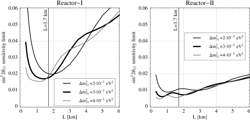
Figure 1: The $\sin^{2}2\theta_{13}$ sensitivity limit as function of the baseline $L$ for the Reactor-I (left plot) and Reactor-II (right plot) setups. It is shown for several values for $\Delta m_{31}^{2}$ at the 90% confidence level. The vertical lines mark the baseline we are using for our standard setups.

We assume a detector technology very similar to the CHOOZ [15] and KamLAND [12] detectors, as well as the Borexino counting test facility [78] (cf., Appendix B). In this work, we suggest a reactor experiment designed to measure $\theta_{13}$. This measurement is based on the ability to detect small spectral distortions in the positron event rates due to neutrino oscillations. For a sensitivity to $\sin^{2}2\theta_{13}$ of the order of $10^{-2}$ this requires a measurement accuracy of about $1\%$. The total experimental uncertainties are, however, considerably larger and come from various sources, such as reactor burn up effects, average neutrino yields, and cross section. In order to control these uncertainties, it is necessary to use a near detector, which accurately determines the energy dependence and total normalization of the neutrino flux [50, 51]. The details of the near detector simulation are described in Appendices A and C. We furthermore do not include backgrounds since, as we discuss in detail in Appendix B, they can be suppressed to a negligible level [79].

We do not propose a specific reactor site in this study and for simplicity we assume a single reactor block. For a given site with several reactors effects like different distances of the cores to near and far detectors or on-off times of the individual reactors have to be included. However, one expects that the main results of this work will also apply in such more complicated situations. We define the integrated luminosity ${\cal L}$ of a reactor experiment in units of fiducial detector mass [tons] $\times$ thermal reactor power [GW] $\times$ running time [years]. In Figure 1, the dependence of the $\sin^{2}2\theta_{13}$ sensitivity on the baseline of the far detector is shown for two values of the integrated luminosity $400\,\mathrm{t}\,\mathrm{GW}\,\mathrm{y}$ (left-hand panel) and $8000\,\mathrm{t}\,\mathrm{GW}\,\mathrm{y}$ (right-hand panel), as well as several values of $\Delta m_{31}^{2}$. It turns out that a baseline of $1.7\,\mathrm{km}$ performs reasonably well for all of the considered cases, which is in agreement with Ref. [51]. This choice is also best for the given uncertainty of $\Delta m_{31}^{2}$ within the atmospheric allowed region, as it lies very close to the optimum for all values of $\Delta m_{31}^{2}$. We assume that the near detector is located at around $0.17\,\mathrm{km}$ in order to avoid oscillation effects. At those very short distances, the contribution of other power stations is far below $1\%$ of the total rate. As long their contribution is known better than to about $10\%$, they do therefore not contribute to the total error to more than $0.1\%$ and we can safely ignore them.

	Reactor-I	Reactor-II
Integrated luminosity	$400\,\mathrm{t}\,\mathrm{GW}\,\mathrm{y}$	$8000\,\mathrm{t}\,\mathrm{GW}\,\mathrm{y}$
Unoscillated events	$31\,493$	$629\,867$
$\sigma_{\mathrm{norm}}$	$0.8\%$	$0.8\%$
$\sigma_{\mathrm{cal}}$	$0.5\%$	$0.5\%$
Baseline	$1.7\,\mathrm{km}$	$1.7\,\mathrm{km}$

Table 1: The most important parameter values of the two reactor benchmark setups Reactor-I and Reactor-II used in this work. For more information see Appendix B.

Throughout this work, we use two experimental benchmark setups labeled as Reactor-I and Reactor-II, which are defined in Table 1. The two values of the integrated luminosity in the table reflect the range of possible experiments with detector masses of the order of $10\,\mathrm{t}$ [50, 51] up to the order of $>100\,\mathrm{t}$ [79, 12]. The near and far detectors are assumed to be identical (maybe apart from their size) in order to minimize the impact of systematical errors. We assume as our standard value for the uncertainty on the event normalization $\sigma_{\mathrm{norm}}=0.8\%$ [51]. This has to be considered as an effective error, receiving contributions from individual uncertainties of the near and far detectors, as well as from over-all flux uncertainties (for details, see Section 4.2 and Appendix A). In addition, we include the effect of an energy calibration error $\sigma_{\mathrm{cal}}=0.5\%$ [15, 80]

3.2 First-generation Superbeams

The two superbeam experiments considered in this study are the JHF to Super-Kamiokande [20] and the NuMI [21] proposals, referred to as “JHF-SK” and “NuMI”. Both projects will use the ${\nu_{\mu}\rightarrow\nu_{e}}$ appearance channel. Neutrino beams which are produced by meson decays always contain irreducible fractions of $\nu_{e}$, $\bar{\nu}_{e}$, and $\bar{\nu}_{\mu}$ contaminations, as well as they have a large high energy tail. Both experiments use therefore an off-axis setup to make the spectrum much narrower in energy and to suppress the beam contaminations [81]. An off-axis beam reaches in this way the low background levels necessary for a good sensitivity to the ${\nu_{\mu}\rightarrow\nu_{e}}$ appearance signal. Both experiments are planned to be operated at nearly the same $L/E$, which is optimized for the first maximum of the atmospheric oscillation for ${\Delta m^{2}_{31}}=3.0\cdot 10^{-3}\,\mathrm{eV}^{2}$.

	JHF-SK	NuMI
Beam
Baseline	$295\,\mathrm{km}$	$712\,\mathrm{km}$
Target Power	$0.77\,\mathrm{MW}$	$0.4\,\mathrm{MW}$
Off-axis angle	$2^{\circ}$	$0.72^{\circ}$
Mean energy	$0.76\,\mathrm{GeV}$	$2.22\,\mathrm{GeV}$
Mean $L/E$	$385\,\mathrm{km}\,\mathrm{GeV}^{-1}$	$320\,\mathrm{km}\,\mathrm{GeV}^{-1}$
Detector
Technology	Water Cherenkov	Low-Z calorimeter
Fiducial mass	$22.5\,\mathrm{kt}$	$17\,\mathrm{kt}$
Running period	5 years	5 years

Table 2: The two superbeams and their detectors as given in Refs. [20, 21]

Due to the different energies of the two beams, different detector technologies are used. For the JHF beam, Super-Kamiokande, a water Cherenkov detector with a fiducial mass of $22.5\,\mathrm{kt}$, is assumed. The Super-Kamiokande detector has an excellent electron muon separation and NC (neutral current) rejection. For the NuMI beam, a low-Z calorimeter with a fiducial mass of $17\,\mathrm{kt}$ is planned, because the hadronic fraction of the energy deposition is much larger at those energies. In spite of the very different detector technologies, their performances in terms of background levels and efficiencies are rather similar. The actual numbers for these quantities and the respective energy resolution of the detectors can be found in [23].

In Ref. [23], several modifications of those setups have been considered in order to improve either the sensitivity to CP violation or to the mass hierarchy. There, it is demonstrated that JHF-SK with about $1/4$ of the total running time with neutrinos and about $3/4$ with antineutrinos performs best for the CP measurement, a setup which is labeled as JHF-SK_cc in this work. However, for the determination of the mass hierarchy the NuMI setup with an increased baseline of $890\,\mathrm{km}$ at an off-axis angle of $0.72^{\circ}$ performs better because of larger matter effects, which will be labeled as NuMI@$890\,\mathrm{km}$ in this work.

4 Measuring $\sin^{2}2\theta_{13}$ at a reactor, and the impact of systematical errors

In this section, we investigate in detail the potential of a reactor experiment to measure $\sin^{2}2\theta_{13}$. In Section 4.1, we discuss obtainable limits on $\sin^{2}2\theta_{13}$, and we present in Sections 4.2 and 4.3 a detailed discussion of systematical errors. The results of these sections are obtained by neglecting correlations of the oscillation parameters, i.e., all parameters except from $\sin^{2}2\theta_{13}$ are fixed to the values given in Equation (3). However, as it can be inferred from the discussion related to Equation (2) and as we will see explicitly in the numerical calculations presented in Sections 5 and 6, the influence of other oscillation parameters on the $\sin^{2}2\theta_{13}$ sensitivity limit from reactors is very small.

4.1 The sensitivity limit to $\sin^{2}2\theta_{13}$

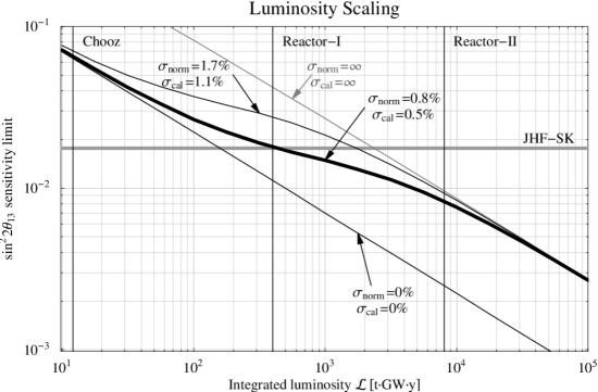
Figure 2: The sensitivity to $\sin^{2}2\theta_{13}$ as a function of the integrated luminosity for different values of the normalization error $\sigma_{\mathrm{norm}}$ and the energy calibration error $\sigma_{\mathrm{cal}}$ at the 90% confidence level, where the thick curve corresponds to our standard values. The vertical lines mark the luminosities of the CHOOZ experiment and our standard setups Reactor-I and Reactor-II as defined in Table 1. The horizontal line shows a typical $\sin^{2}2\theta_{13}$ sensitivity limit obtainable by the JHF-SK superbeam experiment for the same parameter values (taken from Section 5).

We define the sensitivity or sensitivity limit to $\sin^{2}2\theta_{13}$ as the largest value of $\sin^{2}2\theta_{13}$, which is allowed at a given confidence level if the true value is $\sin^{2}2\theta_{13}\equiv 0$. In Figure 2, we show the sensitivity to $\sin^{2}2\theta_{13}$ as a function of the integrated luminosity ${\cal L}$ in units of detector mass [tons] $\times$ thermal reactor power [GW] $\times$ running time [years]. In this figure, the lower diagonal curve corresponds to the idealized case of statistical errors only, and shows just the expected $1/\sqrt{\cal L}$ scaling. Our standard values for the errors on the normalization $\sigma_{\mathrm{norm}}=0.8\%$ and energy calibration $\sigma_{\mathrm{cal}}=0.5\%$ lead to the thick curve, which represents one of the main results of this paper. At a luminosity around $100\,\mathrm{t\,GW\,y}$, we detect a departure from the statistics dominated regime into a flatter systematics dominated region. As discussed in Sections 4.2 and 4.3, this effect is dominated by the error on the normalization $\sigma_{\mathrm{norm}}$, whereas the energy calibration error $\sigma_{\mathrm{cal}}$ only plays a minor role. However, at large luminosities $\gtrsim 10^{4}\,\mathrm{t\,GW\,y}$, the slope of the curve changes, and we are entering again a statistics dominated region with a $1/\sqrt{\cal L}$ scaling. This interesting behavior can be understood as follows: In principle, the far detector measures some combination of the flux normalization and $\sin^{2}2\theta_{13}$. The turnover of the sensitivity line into the second statistics dominated region occurs at the point, where the determination of the normalization by the far detector itself becomes more accurate than the external input $\sigma_{\mathrm{norm}}$. This means that the limit becomes insensitive to the actual value of $\sigma_{\mathrm{norm}}$. We illustrate this by the upper thin black line, which shows the luminosity scaling for the case of larger systematical errors. As an example, we choose values of $\sigma_{\mathrm{norm}}=1.7\%$ for the normalization and $\sigma_{\mathrm{cal}}=1.1\%$ for the energy calibration. We find that, in this case, the transition to the systematics dominated regime occurs at much smaller luminosities. However, for large luminosities, the same limit is approached as for the more optimistic case. The diagonal gray curve shows the limit for no constraint at all on the normalization and energy calibration. Even in this extreme case, we obtain the same limit for high luminosities.

This discussion demonstrates that the magnitude of the systematical error determines the position of the sensitivity plateau, but essentially does not affect the sensitivity at large luminosities. We hence conclude that, for the case of the Reactor-I setup, the systematical normalization error dominates. In order to obtain a reliable limit, it should therefore be well under control. For large luminosities, such as for the Reactor-II setup, the sensitivity limit is independent of normalization errors because of the second statistics dominated regime. The robustness of this result will be further discussed in Section 4.2.

The horizontal line in Figure 2 shows the typical $\sin^{2}2\theta_{13}$ sensitivity limit, which can be obtained from the first-generation JHF-SK superbeam experiment including correlations and degeneracies. It can be inferred that even the Reactor-I experiment gives comparable limits. The competitiveness and complementarity of the information from reactor and superbeam experiments will be discussed in greater detail in Sections 5 and 6. Finally, we note that with a KamLAND-like detector of $1\,\mathrm{kt}$ at a $10\,\mathrm{GW}$ nuclear reactor with a running time of $\sim 5$ years, the high statistic region of a luminosity between $10^{4}\,\mathrm{t\,GW\,y}$ and $10^{5}\,\mathrm{t\,GW\,y}$ seems to be reachable.

4.2 The impact of systematical errors

We discuss now the effects of various systematical errors on the obtainable sensitivity to $\sin^{2}2\theta_{13}$, where technical details are given in Appendix A. Since it is a difficult task to estimate systematical errors of a future experiment, our strategy has been to find realistic values for various normalization errors (e.g., total neutrino flux uncertainty, fiducial mass uncertainty) and energy calibration errors. The chosen numbers are guided by the values obtained in existing reactor experiments, such as the CHOOZ [14, 15] or KamLAND [12] experiments. For other types of errors, such as the shape uncertainty or the experimental systematical error, we have adopted a conservative approach by choosing the worst case situation of completely uncorrelated errors. In detail, we consider the following effects (for the exact definitions, see Appendix A):

1. We take into account a common overall normalization error for the event rates of the near and far detectors. Such an error could, for example, come from the uncertainty of the neutrino flux normalization or the error on the detection cross section. Typically, it is of the order of a few percent.

2. We include uncorrelated normalization uncertainties of the near and far detectors. Here contributes, for instance, the error on the fiducial mass of each detector. We assume that in this case an error below 1% can be reached.

3. We take into account the energy calibration uncertainty by introducing a parameter $g^{A}$ for each detector ($A=N,F$), and replace the observed energy $E_{\mathrm{obs}}$ by $(1+g^{A})E_{\mathrm{obs}}$. We assume that the energy calibration is known within an error of $\sigma_{\mathrm{cal}}\sim 0.5\%$.

4. In order to take into account an uncertainty of the shape of the expected energy spectrum, we introduce an error $\sigma_{\mathrm{shape}}$ on the theoretical prediction for each energy bin which is completely uncorrelated between different energy bins. This corresponds to the most pessimistic assumption of no knowledge of possible shape distortions. However, we choose this error fully correlated between the corresponding bins in the near and far detector, since shape distortions should affect the signals in both detectors of equal technology in the same way.

5. We include the possibility of an uncorrelated experimental systematical error $\sigma_{\mathrm{exp}}$. Such an error could, for example, result from insufficient knowledge of some source of background. We call this uncertainty “bin-to-bin error” and take it completely uncorrelated between energy bins, as well as between the near and far detectors. Note that this corresponds again to the worst case scenario, and values of $\sigma_{\mathrm{exp}}$ at the per mill level should be realistic.

As it is explicitely demonstrated in Appendix A, the overall normalization error, the individual normalization errors of the two detectors, and the energy calibration error of the near detector can be merged into an effective normalization error $\sigma_{\mathrm{norm}}$ for the far detector. Assuming realistic values of 2% [15] for the total normalization uncertainty and 0.6% [80] for the detector-specific uncertainty, we obtain from Equations (18) and (19) in Appendix A an effective normalization error of $\sigma_{\mathrm{norm}}=0.8\%$, which is the standard value for our numerical calculations.

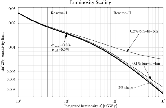
Figure 3: The sensitivity to $\sin^{2}2\theta_{13}$ as a function of the integrated luminosity for several selected error sources at the 90% confidence level. The thick curve corresponds to our standard values for the errors on the flux normalization and the energy calibration. The gray curve has been calculated by adding an error of 2% for the shape of the predicted energy spectrum. For the curves labeled with “bin-to-bin”, we include an uncorrelated experimental systematical error as given by the corresponding label. The vertical lines mark the integrated luminosities of our standard setups Reactor-I and Reactor-II as defined in Table 1.

The impact of a spectral shape uncertainty and of experimental systematical errors is illustrated in Figure 3, where we show the luminosity scaling of the $\sin^{2}2\theta_{13}$-limit for some values of these errors. The curve labeled with “2% shape” corresponds to an uncorrelated shape error on the predicted energy spectrum, such as it is described in item 4 above. This error covers a large class of systematical effects, such as the uncertainty on the $\beta$-decay spectrum of various isotopes in the reactor, uncertainties of the fuel composition, or burn-up effects. As it can be inferred from the figure, such an error has very little impact on the sensitivity limit. The reason for this is that shape uncertainties can be reduced very efficiently by the near detector, assuming that there are at least 10 times more events in the near detector than in the far detector. Our assumption of an uncorrelated error is the most pessimistic theoretical error one could imagine. In more realistic cases, one may expect some correlation of the shape uncertainty between the energy bins, which could be even better eliminated by the near detector.

The presence of a systematical, experimental bin-to-bin uncorrelated error, as described in item 5, is potentially more problematic for the measurement than any other error, since it cannot be eliminated with the help of the near detector. As it is shown in Figure 3, such an error with a value below 0.5% has no effect for the Reactor-I setup, but it spoils the statistics dominated region at high luminosities and would be important for large detectors, such as Reactor-II. However, we note that 0.5% for an uncorrelated error of this type is a relatively large number, which should be reducible down to the 0.1% level. In this region, the impact on the $\sin^{2}2\theta_{13}$-limit becomes very small. Suppose, for example, that the number of background events in the detector is 1% of the reactor neutrino events. In this case, a 10% knowledge of this background is sufficient to reach a 0.1% error on the experimental event rate.

4.3 Normalization and energy calibration errors, and the impact of an energy cut

Since we have already demonstrated that the impact of an error on the expected energy shape is very small, we will neglect it for the rest of this work. Moreover, we further on assume that the experimental bin-to-bin uncorrelated systematical error can be reduced to the 0.1% level and hence can also be neglected. Then, as shown in Appendix A, all systematical effects considered in this paper can be reduced to two systematical errors, which are the effective normalization uncertainty $\sigma_{\mathrm{norm}}$ and the energy calibration error $\sigma_{\mathrm{cal}}$ in the far detector. We will discuss now in this subsection the impact of these two errors in greater detail, combined with a possible low energy cut which could be required in some cases to eliminate backgrounds.

Figure 4: The sensitivity to $\sin^{2}2\theta_{13}$ for the Reactor-I and Reactor-II setups at the 90% confidence level. The left vertical line in each bar corresponds to statistical errors only, whereas the right edge shows the limit for different combinations of normalization and calibration errors. The sensitivity limits are shown for $\sigma_{\mathrm{norm}}=0.8\%$ and $\sigma_{\mathrm{cal}}=0.5\%$, or for $\sigma_{\mathrm{norm}}=\sigma_{\mathrm{cal}}\to\infty$ where indicated explicitly. Furthermore, the sensitivity limits are shown without cut on the energy, and for an energy cut at $E_{\nu}\geq 3.4\,\mathrm{MeV}$.

In Figure 4, we illustrate the $\sin^{2}2\theta_{13}$ sensitivity limits for various values of $\sigma_{\mathrm{norm}}$ and $\sigma_{\mathrm{cal}}$. The vertical lines at the left edge of each bar correspond to the idealized case of statistical errors only. The bars indicate, how the limit deteriorates by including either the normalization error or the calibration error or both. Let us first focus on the cases labeled “no cut”, where the full energy range of $1.8\,\mathrm{MeV}\leq E_{\nu}\leq\mathrm{8}\,\mathrm{MeV}$ is considered. The final sensitivity limit is dominated by the normalization error, and the calibration error has a rather small impact, although it is not negligible. We also show in Figure 4 the extreme case, where $\sigma_{\mathrm{norm}}$ and $\sigma_{\mathrm{cal}}$ are set to infinity, i.e., the event normalization and the energy scale are treated as free parameters in the fit (cf., Equation (17) in Appendix A). We learn from this analysis that for $\sigma_{\mathrm{cal}}>0$ only, even if we include the energy scale as a free parameter in the fit, the limit is essentially the same as the pure statistics limit. This demonstrates again that an energy scale uncertainty is not very important. In addition, we observe that for Reactor-I the final sensitivity limit is significantly worse for $\sigma_{\mathrm{norm}}=\sigma_{\mathrm{cal}}\to\infty$ than for $\sigma_{\mathrm{norm}}=0.8\%$, $\sigma_{\mathrm{cal}}=0.5\%$, whereas the limits for Reactor-II are essentially unchanged. This again illustrates the effect already discussed earlier in the context of Figure 2: At high luminosities the oscillation signal is dominated by the spectral information and the far detector itself provides an accurate measurement of the overall flux, which means that the $\sin^{2}2\theta_{13}$ sensitivity limit becomes insensitive to the value of $\sigma_{\mathrm{norm}}$. On the contrary, for lower luminosities, such as for the Reactor-I setup, a precise knowledge on $\sigma_{\mathrm{norm}}$ is rather important, and the limit can be significantly improved for small normalization errors.

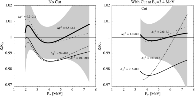
Figure 5: The ratio of the event rates at the $3\sigma$ limit of $\sin^{2}2\theta_{13}$ to the event rates for $\sin^{2}2\theta_{13}=0$ for Reactor-II ($\sin^{2}2\theta_{13}=1.5\cdot 10^{-2}$ in the left plot and $\sin^{2}2\theta_{13}=2.5\cdot 10^{-2}$ in the right plot). In the left-hand panel, the full energy range is included, whereas in the right-hand panel, an energy cut at $E_{\nu}\geq 3.4\,\mathrm{MeV}$ is imposed. The thin solid curves correspond to the case of no systematical errors, whereas the long-dashed curves correspond to a calibration error of $\sigma_{\mathrm{cal}}=0.5\%$, the short-dashed curves to a normalization error of $\sigma_{\mathrm{norm}}=0.8\%$, and the thick solid curves to both errors switched on simultaneously. The shaded regions show the statistical errors, and the numbers given for each curve correspond to the separate contribution to the total value of $\Delta\chi^{2}$ of the data and the systematical errors, see Equation (17).

The cases in Figure 4 labeled “with cut” correspond to the situation when a low energy cut is imposed. Such a cut could be motivated by some low energy background, such as from radioactivity of the detector material [15]. For illustration, we have chosen the cut $E_{\nu}\geq 3.4\,\mathrm{MeV}$ corresponding to $E_{\mathrm{vis}}\geq 2.6\,\mathrm{MeV}$, as it is applied in the KamLAND experiment to avoid the contribution of geo-neutrinos. Apart from the slight worsening of the statistics-only limit due to smaller event numbers, we find that the cut has a rather drastic impact for the large detector Reactor-II. The reason for this effect is illustrated in Figure 5, where we show the normalized energy spectrum for the following four cases: no systematical errors, either $\sigma_{\mathrm{norm}}$ or $\sigma_{\mathrm{cal}}$ included, and both $\sigma_{\mathrm{norm}}$ and $\sigma_{\mathrm{cal}}$ simultaneously included. One can see that the cut at $3.4\,\mathrm{MeV}$ is close to the oscillation minimum at this baseline of $1.7\,\mathrm{km}$. For such an unfortunate choice, the interplay of normalization and calibration can very efficiently reduce the oscillation pattern in the spectrum by making the signal essentially flat. In fact, we have found that, in the presence of an energy cut, our standard values for $\sigma_{\mathrm{norm}}$ and $\sigma_{\mathrm{cal}}$ are sufficient to completely destroy the statistics dominated regime at high luminosities, similar to the “bin-to-bin” error shown in Figure 3. This problem can be avoided by making sure that the oscillation minimum is safely included inside the accessible energy range, such as for the case when no cut is applied. With this choice, it is impossible to destroy the oscillation signature by shifting the normalization or stretching the energy scale, as it is clear from the left plot of Figure 5. If a low energy cut cannot be avoided because of backgrounds, one should eventually consider to change the baseline in order to make sure that the oscillation minimum is covered by the remaining energy window.

5 The measurement of $\sin^{2}2\theta_{13}$: reactors versus superbeams

In this section, we compare the potential to measure $\sin^{2}2\theta_{13}$ in reactor experiments with the one of superbeams. As far as $\sin^{2}2\theta_{13}$ is concerned, we will demonstrate that even the small reactor setup Reactor-I can compete with a first-generation superbeam, such as JHF-SK or NuMI. There are essentially two interesting measurements for $\sin^{2}2\theta_{13}$: the sensitivity to $\sin^{2}2\theta_{13}$ and the precision of the measurement of $\sin^{2}2\theta_{13}$. The discussion is therefore divided into two parts, where we also define the respective quantities.

5.1 The sensitivity to $\sin^{2}2\theta_{13}$

We define the sensitivity or sensitivity limit to $\sin^{2}2\theta_{13}$ as the largest value of $\sin^{2}2\theta_{13}$, which fits the true value $\sin^{2}2\theta_{13}\equiv 0$ at the chosen confidence level. For an experiment or a combination of experiments, it reflects the range between the sensitivity limit and the CHOOZ bound, where $\sin^{2}2\theta_{13}>0$ could be detected. With this definition, it should be clear that especially for superbeams the $\mathrm{sgn}(\Delta m_{31}^{2})$-degeneracy has to be taken into account in the calculations, since the degenerate solution at $-|\Delta m_{31}^{2}|$ may allow a larger value of $\sin^{2}2\theta_{13}$ fitting $\sin^{2}2\theta_{13}\equiv 0$ than the best-fit solution. In addition, it has been demonstrated in Ref. [23] that with this definition the sensitivity limits for the normal and inverted mass hierarchies are equal for the superbeams, since the zero rate vectors for the appearance channel are equal for $\sin^{2}2\theta_{13}\equiv 0$. Similarly, Equation (2) does not depend on the sign of $\Delta m_{31}^{2}$, which means that the sensitivity limit does not depend on the type of the hierarchy in this case, either.

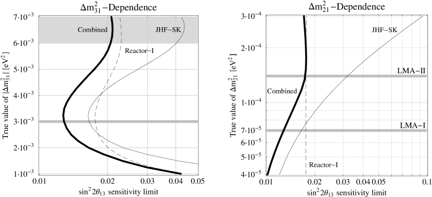
Figure 6: The sensitivity limits to $\sin^{2}2\theta_{13}$ as functions of the true values of $\Delta m_{31}^{2}$ (left plot) or $\Delta m_{21}^{2}$ (right plot), respectively. They are shown for the JHF-SK and Reactor-I setups as well as their combination at the $90\%$ confidence level. In the left figure, the atmospheric excluded region is shaded in gray, and in the right figure, only the KamLAND-allowed region is shown. In both figures, the best-fit values are marked by the gray lines.

Figure 6 shows the sensitivity limits for JHF-SK as example for the superbeams and Reactor-I, as well as their combination at the $90\%$ confidence level. In this figure, the left plot represents the $\Delta m_{31}^{2}$-dependence and the right plot the $\Delta m_{21}^{2}$-dependence. In order to compare experiments with similar capabilities, we have chosen the Reactor-I setups for these plots. The Reactor-II setup would be much better and would dominate the result.

For the best-fit parameters used in this work, we obtain a sensitivity limit of $\sin^{2}2\theta_{13}\simeq 1.8\cdot 10^{-2}$ for Reactor-I at the $90\%$ confidence level, as it can be read off from the figure. This result is in rather good agreement with the setups in Refs. [51] and [50], where similar values for the systematics uncertainties were used. In Figure 6, the $\Delta m_{31}^{2}$-dependence clearly reflects the fact that both the JHF-SK and Reactor-I experiments are optimized for a value of $\Delta m_{31}^{2}\simeq 3.0\cdot 10^{-3}\,\mathrm{eV}^{2}$. However, as we have seen in Figure 1, the broad reactor spectrum does not make this optimization peak as sharp as in the superbeam case, where the off-axis technology is actually used to produce a narrow-band beam. The risk of choosing a non-optimal value for the $\Delta m_{31}^{2}$-optimization within the atmospheric allowed region is therefore much lower in the reactor case, though the superbeam is marginally better at the best-fit value. From the combination of the two experiments, we do not observe synergy effects which would improve the performance beyond a simple addition of statistics. As it is demonstrated in Figure 3 of Ref. [23], the NuMI setup would lead to very similar results.

As far as the $\Delta m_{21}^{2}$-dependence is concerned, superbeams strongly suffer from the correlation with the CP phase. This can already be seen in Equation (1), where especially for large values of the hierarchy parameter $\alpha\equiv\Delta m_{21}^{2}/\Delta m_{31}^{2}$ the second and third terms become larger, and $\sin^{2}2\theta_{13}$ becomes highly correlated with $\delta_{\mathrm{CP}}$. Thus, the JHF-SK setup loses almost any sensitivity to $\sin^{2}2\theta_{13}$ below the CHOOZ bound for large values of $\Delta m_{21}^{2}$ within the LMA-allowed region, as it can be seen in the right plot of Figure 6. On the other side, the reactor setup is hardly influenced by $\alpha$, since for the short baseline the effects of $\alpha$ within the LMA-allowed region are small. Thus, though a little bit worse for small values of $\Delta m_{21}^{2}$, Reactor-I has a much better sensitivity than JHF-SK in most of the LMA-allowed region. The combination of the two experiments does, as in the case of $\Delta m_{31}^{2}$, not show significant synergy effects beyond adding the statistics of the two experiments.

Apart from $\sin^{2}2\theta_{13}$, the reactor experiment is sensitive to some parameters which can be more precisely measured by earlier experiments. We have therefore imposed external information on the parameters $\Delta m_{31}^{2}$, $\Delta m_{21}^{2}$, and $\sin^{2}2\theta_{12}$ appearing in Equation (2), and have studied the dependencies on the precision of this information. We find that the reactor experiment itself can measure the relevant parameters with a sufficient precision, as long as $\Delta m_{31}^{2}$ is known better than to $30\%-50\%$ from external measurements. This required external precision of $\Delta m_{31}^{2}$ is easily achievable by conventional beam experiments, such as CNGS, MINOS, or K2K. The Reactor-I setup is in summary very competitive to the first-generation superbeams, especially since the risk of the unknown parameter values of $\Delta m_{31}^{2}$ and $\Delta m_{21}^{2}$ is considerably lower. With a higher luminosity, the Reactor-II setup could moreover do much better than the first-generation superbeams on comparable timescales.

5.2 The precision of $\sin^{2}2\theta_{13}$

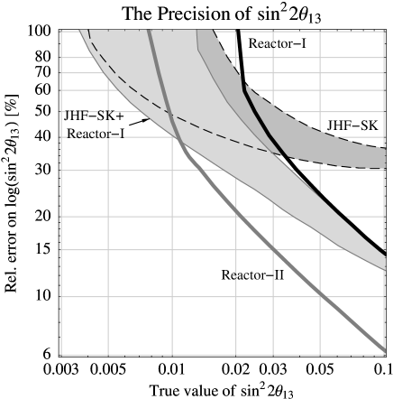
Figure 7: The relative error on $\mathrm{log}(\sin^{2}2\theta_{13})$ defined in Equation (7) as function of the true value of $\sin^{2}2\theta_{13}$ for JHF-SK, Reactor-I, Reactor-II, and the combination of JHF-SK and Reactor-I at the $90\%$ confidence level. For experiments or combinations involving JHF-SK, the (by then unknown) true value of $\delta_{\mathrm{CP}}$ leads to bands representing all possible values of $\delta_{\mathrm{CP}}$. In addition, for each value of $\delta_{\mathrm{CP}}$, the worst among the best-fit and degenerate solutions was chosen.

As soon as $\sin^{2}2\theta_{13}\neq 0$ is established by an experiment, the obtainable precision of $\sin^{2}2\theta_{13}$ becomes interesting. This precision of the measurement of $\sin^{2}2\theta_{13}$ depends, of course, on the true value of $\sin^{2}2\theta_{13}$ itself. A meaningful quantity to discuss this precision is the relative error on $\mathrm{log}(\sin^{2}2\theta_{13})$ as a function of $\sin^{2}2\theta_{13}$ [40], i.e.,

$$\mathrm{Rel.\,error\,on\,}\mathrm{log}(\sin^{2}2\theta_{13})\,\,[\%]\equiv\frac{|\mathrm{log}(\sin^{2}2\theta_{13}^{(2)})-\mathrm{log}(\sin^{2}2\theta_{13}^{(1)})|}{\mathrm{log}(\sin^{2}2\theta_{13})}\cdot 100.$$ (7)

Here $\mathrm{log}(\sin^{2}2\theta_{13}^{(2)})$ and $\mathrm{log}(\sin^{2}2\theta_{13}^{(1)})$ refer to the upper and lower intersections, respectively, of the $\chi^{2}$-function with the $90\%$ confidence level. With this definition, it should be obvious that this relative error becomes larger than $100\%$ close to the sensitivity limit. It is shown in Figure 7 for JHF-SK and Reactor-I, their combination, and Reactor-II. For any combination with a superbeam, we included in this calculation the degenerate solutions by taking the largest relative error of all degenerate solutions. In addition, we made no special assumptions about the unknown CP phase, which leads to the bands for experiments involving the superbeam in Figure 7. The lower edge of these bands corresponds to the best case, the upper edge to the worst case. This form of visualization takes into account that we do not know by then, which true value of $\delta_{\mathrm{CP}}$ has been realized by nature. The different results for different values of $\delta_{\mathrm{CP}}$ originate in the different shapes of the $\delta_{\mathrm{CP}}$-$\theta_{13}$-correlation, which means that this dependence does not necessarily imply that the experiment can measure $\delta_{\mathrm{CP}}$.

From Figure 7, we find that the precision of $\sin^{2}2\theta_{13}$ is much better for the reactor experiments for large values of $\sin^{2}2\theta_{13}$, but for small values of $\sin^{2}2\theta_{13}$ the superbeams become better. This behavior stems from the different nature of the signals: the reactor experiments measure $\theta_{13}$ in the disappearance channel, whereas the superbeams measure the appearance of events. For reactor experiments, the statistical and systematical errors are therefore basically independent of $\sin^{2}2\theta_{13}$, which implies that the precision of $\sin^{2}2\theta_{13}$ vanishes for small values of $\sin^{2}2\theta_{13}$. On the other hand, superbeams have, even for large values of $\sin^{2}2\theta_{13}$, only a limited number of signal events [40]. Therefore, the statistical errors are relatively large compared to a reactor experiment. For smaller values of $\sin^{2}2\theta_{13}$, however, the relative statistical error decreases as $1/\sqrt{N}$. This results in a much better accuracy at low values of $\sin^{2}2\theta_{13}$. The same loss of precision for reactor experiments can also be observed in the $\sin^{2}2\theta_{13}$-$\Delta m_{31}^{2}$-plane, as shown in Figure 2 of Ref. [51]. This figure illustrates that under a certain threshold value for $\sin^{2}2\theta_{13}$ the shape of the $\sin^{2}2\theta_{13}$-$\Delta m_{31}^{2}$ allowed region changes dramatically. Another consequence of the shape of this region is that an external measurement of $\Delta m_{31}^{2}$ does not influence the precision of $\sin^{2}2\theta_{13}$ in Figure 7 very much, because for large values of $\sin^{2}2\theta_{13}$ the parameters $\Delta m_{31}^{2}$ and $\sin^{2}2\theta_{13}$ are uncorrelated, and for small values of $\sin^{2}2\theta_{13}$ the relative error as defined in this section quickly becomes very large before $\Delta m_{31}^{2}$ and $\sin^{2}2\theta_{13}$ become highly correlated.

As far as the combination of Reactor-I and JHF-SK is concerned, there is some synergy for small values of $\sin^{2}2\theta_{13}$. Though the precision of the reactor experiment deteriorates, both experiments together are somewhat better than the superbeam alone. The Reactor-II setup is however much better, even better than the combination of Reactor-I with JHF-SK for large values of $\sin^{2}2\theta_{13}$, which means that a larger detector can really help in this case. After all, the superbeam suffers from the same problem as for the sensitivity limit: the larger $\Delta m_{21}^{2}$ is, the worse the precision of $\sin^{2}2\theta_{13}$ becomes. An unfortunate true value of the CP phase would additional erode the performance. Contrary to that, the Reactor-II setup does not have these problems, which means that a reactor experiment with a large detector would be the optimal choice to measure $\sin^{2}2\theta_{13}$ with lower risks coming from oscillation parameter uncertainties.

6 The complementarity of reactor experiments and superbeams

We have already seen that the reactor experiments are very competitive in measuring $\sin^{2}2\theta_{13}$. There are, however, other parameters, which the reactor experiments cannot access satisfactorily, such as the sign of $\Delta m_{31}^{2}$ and CP violation. We will therefore demonstrate now, how the reactor experiments would fit in the larger picture of the next-generation experiments. We will use the Reactor-II setup to identify the optimal combinations with the first-generation superbeams. This will demonstrate what reactor experiments can contribute in the best case.

6.1 Precision measurements of the leading atmospheric parameters

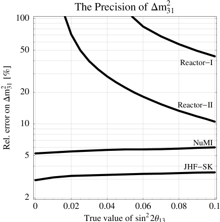
Figure 8: The relative error on $\Delta m_{31}^{2}$ in percent as function of the true value of $\sin^{2}2\theta_{13}$ for JHF-SK, NuMI, Reactor-I, and Reactor-II. For the calculation of the error, the full width of the $\chi^{2}$-function in the best-fit region is taken at the 90% confidence level.

Among the interesting parameters for superbeams are the leading atmospheric parameters $\Delta m_{31}^{2}$ and $\sin^{2}2\theta_{23}$. Compared to conventional beams, such as K2K, CNGS, and MINOS, the superbeams could achieve very high precisions for the leading atmospheric parameters. Reactor experiments are, at the short baselines we are considering, besides $\sin^{2}2\theta_{13}$, only sensitive to $\Delta m_{31}^{2}$. This can be understood in terms of Equation (2): the atmospheric mixing angle $\theta_{23}$ does not even appear in this equation and the sensitivity to the leading solar parameters can only be sensibly achieved at longer baselines, where $\Delta_{21}$ is large enough. Therefore, the first-generation superbeams would supply a measurement without serious competition at least for $\sin^{2}2\theta_{23}$. The atmospheric mass squared difference $\Delta m_{31}^{2}$, however, could be measured by superbeams as well as reactor experiments, as it is illustrated in Figure 8. There is nevertheless one important difference between those two types of experiments. The superbeams measure $\Delta m_{31}^{2}$ with the disappearance channels, which are dominated by the leading atmospheric oscillation, and the measurement thus hardly depends on the true value of $\sin^{2}2\theta_{13}$. For the reactor experiments, though, the parameter $\Delta m_{31}^{2}$ is part of the signal proportional to $\sin^{2}2\theta_{13}$. Therefore, they are strongly affected by the true value of $\sin^{2}2\theta_{13}$, as it is demonstrated in Figure 8. We hence conclude that long-baseline experiments are very important for precision measurements of the leading atmospheric parameters independent of the true value of $\sin^{2}2\theta_{13}$.

6.2 The sensitivity to the sign of $\Delta m_{31}^{2}$

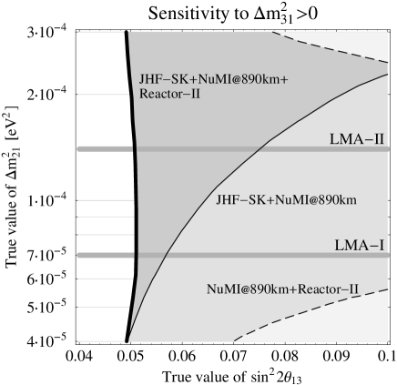
Figure 9: The sensitivity to a positive sign of $\Delta m_{31}^{2}$ (normal mass hierarchy) as function of the true values of $\sin^{2}2\theta_{13}$ and $\Delta m_{21}^{2}$ within the KamLAND-allowed region. Sensitivity at the 90% confidence level exists on the right-hand sides of the curves. It is shown for several combinations of experiments: for JHF-SK combined with NuMI at a baseline of $890\,\mathrm{km}$ [23], for NuMI at a baseline of $890\,\mathrm{km}$ combined with Reactor-II, and for JHF-SK combined with NuMI at a baseline of $890\,\mathrm{km}$ and Reactor-II. The LMA best-fit values are marked by the horizontal gray lines.

As it has been demonstrated in Refs. [40, 23] and elsewhere, the mass hierarchy is, due to the $\mathrm{sgn}(\Delta m_{31}^{2})$-degeneracy, one of the hardest parameters to access for future long-baseline experiments. As it can be seen in Equation (1), the opposite sign of $\Delta m_{31}^{2}$ opens, especially for large $\Delta m_{21}^{2}$, the possibility of a degenerate solution at a different value of $\delta_{\mathrm{CP}}$, which makes it very hard to determine the mass hierarchy. We define that an experiment is sensitive to a certain sign of $\Delta m_{31}^{2}$, if there is no possible solution with the opposite sign of $\Delta m_{31}^{2}$ below the chosen confidence level. This sensitivity depends, similarly to the precision of $\sin^{2}2\theta_{13}$, on the unknown true value of $\delta_{\mathrm{CP}}$. We take therefore the most conservative value of $\delta_{\mathrm{CP}}$ in order to show where sensitivity to the tested hierarchy exists independent of $\delta_{\mathrm{CP}}$. With this definition, it can be shown that neither the first-generation superbeams, such as NuMI or JHF-SK, nor their combination, do have any sensitivity to the mass hierarchy [23]. However, because of matter effects, which increase with the baseline, and the ability to resolve degeneracies with the combination of two superbeams [45, 23], the combination of NuMI at a longer baseline together with JHF-SK is sensitive to the sign of $\Delta m_{31}^{2}$ in a large region of the $\sin^{2}2\theta_{13}$-$\Delta m_{21}^{2}$-plane. The result for a positive sign of $\Delta m_{31}^{2}$ and the combination of JHF-SK with NuMI at a baseline of $890\,\mathrm{km}$ from Ref. [23] is, for example, shown in Figure 9. As it can be seen in the figure, the sensitivity to the normal mass hierarchy vanishes for large values of $\Delta m_{21}^{2}$, which mainly comes from the $\mathrm{sgn}(\Delta m_{31}^{2})$-degeneracy.

We find however that the combination of the Reactor-II setup at the short baseline of $1.7\,\mathrm{km}$ with two superbeam experiments significantly improves the sensitivity to the mass hierarchy. Figure 9 demonstrates that this combination (thick solid curve) has a very good sensitivity to $\Delta m_{31}^{2}>0$ which does not depend on $\Delta m_{21}^{2}$. The reactor experiment helps here indirectly to resolve the $\mathrm{sgn}(\Delta m_{31}^{2})$-degeneracy by the precision measurement of $\sin^{2}2\theta_{13}$. The combination of the three experiments thus leads to a much better sensitivity to the normal mass hierarchy at large values of $\Delta m_{21}^{2}$ within the LMA-allowed region. In order to demonstrate that one superbeam plus the reactor experiment at the short baseline is not enough to access the mass hierarchy, we show, in addition, in Figure 9 the combination of the superbeam with the larger matter effects, i.e., NuMI at $890\,\mathrm{km}$, together with Reactor-II. Figure 9 is for a normal mass hierarchy, but the inverted mass hierarchy produces rather similar results [23].

In Ref. [82], it has been pointed out that for the case of a relatively large $\Delta m_{21}^{2}$, a reactor neutrino experiment at a baseline of the order of 30 km might have some sensitivity to the sign of $\Delta m_{31}^{2}$ because of an interference term between $\Delta m_{21}^{2}$ and $\Delta m_{31}^{2}$ (see also Ref. [79]). This interference term is of third order proportional to $\alpha\cdot\sin^{2}2\theta_{13}$, which means that it does not appear in our Equation (2). According to our numerical results, a determination of the mass hierarchy at the $90\%$ confidence level based on this effect is not possible, even for a combination of two big reactor experiments with luminosities of $10^{5}\,\mathrm{t\,GW\,y}$ at baselines of $1.7\,\mathrm{km}$ and $30\,\mathrm{km}$. In order to observe this tiny effect, the ratio $\Delta m_{21}^{2}/\Delta m_{31}^{2}$ and $\sin^{2}2\theta_{13}$ should be as large as possible, and the solar mixing has to be far from maximal mixing. Moreover, all these parameters have to been know with (unrealistically) high precisions.

6.3 The sensitivity to CP violation

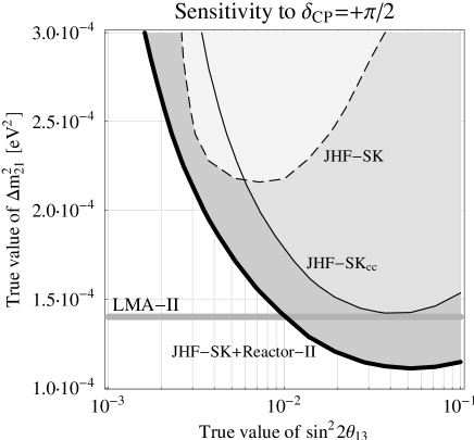
Figure 10: The sensitivity to maximal CP violation $\delta_{\mathrm{CP}}=+\pi/2$ as function of the true values of $\sin^{2}2\theta_{13}$ and $\Delta m_{21}^{2}$ within the KamLAND-allowed region. The sensitivity is at the 90% confidence level given on the upper sides of the curves. It is shown for JHF-SK (neutrino running only), JHF-SK_cc (same overall running time split into neutrino and antineutrino running with about equal numbers of events), and JHF-SK (neutrino running only) combined with Reactor-II. The LMA-II best-fit value is marked by the horizontal gray line.

There are various approaches to evaluate the capability of an experiment to access $\delta_{\mathrm{CP}}$. One of those, which is quite intuitive to understand and qualitatively representative, is the sensitivity to maximal CP violation $\delta_{\mathrm{CP}}=\pm\pi/2$. In this spirit, we define that an experiment (or a combination) is sensitive to maximal CP violation, if the true value $\delta_{\mathrm{CP}}=\pm\pi/2$ does not fit the CP conserving values $0$ and $\pi$ at the chosen confidence level. With this definition, it is obvious that also the degenerate solutions have to be tested, since any degenerate solution with $\delta_{\mathrm{CP}}=0$ or $\pi$ fitting the maximal CP violation would destroy the sensitivity. It has been demonstrated in Ref. [23] that for the first-generation superbeams the results qualitatively do not depend very much on the choice of the normal or inverted mass hierarchy and the true value $\delta_{\mathrm{CP}}=+\pi/2$ or $\delta_{\mathrm{CP}}=-\pi/2$. We show therefore only the results for the normal hierarchy and $\delta_{\mathrm{CP}}=+\pi/2$ in this work. In addition, it has been discussed in Refs. [45, 23] and elsewhere that for the detection of CP violation with superbeams a combined neutrino and antineutrino running is very important – either within one superbeam experiment or in the combination of different superbeams with different polarities. This result is not very surprising, since those two channels have a complementary dependence on the CP phase (cf., Equation (1)) and their combination helps to resolve the correlation between $\sin^{2}2\theta_{13}$ and $\delta_{\mathrm{CP}}$. The antineutrino running has, however, one disadvantage: in order to accumulate similar event rates for comparable statistical weights, the antineutrino mode has to be operated much longer than the neutrino mode to compensate the lower cross section of antineutrinos. As illustrated for different setups in Figure 10, there is a possibility to circumvent this problem with JHF-SK. Instead of resolving the correlation between $\sin^{2}2\theta_{13}$ and $\delta_{\mathrm{CP}}$ with the antineutrino channel, one could as well resolve it with a precision measurement of $\sin^{2}2\theta_{13}$ with a reactor experiment. The JHF-SK setup is in Figure 10 shown in three different configurations: alone with neutrino running only (JHF-SK), alone with the total running time split in order to obtain about equal numbers of neutrino and antineutrino events (JHF-SK_cc), and in combination with Reactor-II with neutrino running only (JHF-SK+Reactor-II). The combined neutrino-antineutrino running at JHF-SK_cc clearly helps to improve the performance compared to running with neutrinos only (JHF-SK). There is, however, only a marginal improvement by adding the reactor experiment to JHF-SK_cc. The reason is that the correlation between $\sin^{2}2\theta_{13}$ and $\delta_{\mathrm{CP}}$ is in this case already resolved by the antineutrino channel, and a precision measurement of $\sin^{2}2\theta_{13}$ does not improve the sensitivity to CP violation further. The third, most interesting case in Figure 10 shows the combination of JHF-SK with neutrino running only with Reactor-II. Because the statistics for JHF-SK is much better than for the combined neutrino and antineutrino running here, and the correlation between $\sin^{2}2\theta_{13}$ and $\delta_{\mathrm{CP}}$ can be resolved by the reactor experiment, the overall performance is optimal. It even covers the LMA-II best-fit value, which leads to the interesting chance to observe leptonic CP violation by such a combination. We have not found any other combination (e.g., involving two superbeams as in Ref. [23]), which could achieve such a good coverage in the $\sin^{2}2\theta_{13}$-$\Delta m_{21}^{2}$-plane by using the first-generation JHF-SK and NuMI superbeams. Especially, the CP performance of NuMI suffers from the fact that mainly the first term in Equation (1) is enhanced by matter effects, which means that the relative weight of the second and third CP-sensitive terms is lower than in the JHF-SK case. A reactor experiment could thus be a very important element to measure $\delta_{\mathrm{CP}}$ without including an antineutrino running at superbeams. This is, however, because of the limited statistics, for the first-generation superbeam experiments restricted to the LMA-II region.

7 Summary and conclusions

We have presented a detailed study of potential reactor experiments with near and far detectors. The first important aspect covered by this study has been a careful modeling and discussion of the systematical errors of such reactor experiments. The second major issue has been the comparison to the first-generation superbeams JHF-SK (JHF to Super-Kamiokande) and NuMI  and the study of complementary effects between reactor experiments and superbeams. For a quantitative discussion, we have defined benchmark reactor experiments with far detectors up to the size of the KamLAND detector, which we have labeled as Reactor-I and Reactor-II. They have integrated luminosities of $400\,\mathrm{t\,GW\,y}$ and $8\,000\,\mathrm{t\,GW\,y}$, respectively, where the units are given as detector mass [tons] $\times$ thermal reactor power [GW] $\times$ running time [years].

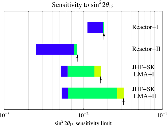
Figure 11: The sensitivity to $\sin^{2}2\theta_{13}$ for Reactor-I, Reactor-II, JHF-SK at LMA-I ($\Delta m_{21}^{2}=7\cdot 10^{-5}\,\mathrm{eV}^{2}$), and JHF-SK at LMA-II ($\Delta m_{21}^{2}=1.4\cdot 10^{-4}\,\mathrm{eV}^{2}$) at the $90\%$ confidence level. The sensitivitiy limits for the reactor experiments hardly depend on the true value of the solar parameters. The left edges of the bars correspond to the sensitivity limits from statistics only, the right edges of the bars to the real sensitivity limits after successively switching on systematics (dark/blue), correlations (medium gray/green), and degeneracies (light gray/yellow).

The structure of the relevant oscillation probabilities of reactor experiments demonstrates that they are only very little spoilt by correlations and not at all by degeneracies (cf., Section 2). Very good sensitivity limits for $\sin^{2}2\theta_{13}$ can therefore be obtained. For our setups, we find, for the current best-fit values, sensitivity limits of $\sin^{2}2\theta_{13}\simeq 1.8\cdot 10^{-2}$ (Reactor-I) and $\sin^{2}2\theta_{13}\simeq 7.6\cdot 10^{-3}$ (Reactor-II), which is a significant improvement of the current CHOOZ bound. Compared to the superbeams, the Reactor-I sensitivity limit corresponds to the JHF-SK experiment including systematics, correlations, and degeneracies, which is about $\sin^{2}2\theta_{13}\simeq 1.7\cdot 10^{-2}$ for the LMA-I solution. The dependence of the sensitivity limits of Reactor-I, Reactor-II, and JHF-SK on systematics, correlations, and degeneracies is illustrated in Figure 11. Compared to the superbeams, the sensitivities of the reactor experiments are almost unaffected by the true values of the solar parameters and less dependent on the value of $\Delta m_{31}^{2}$. The dependence of the superbeam sensitivity limit on the LMA-I or LMA-II solution is shown in Figure 11, whereas the reactor experiments are hardly affected by $\Delta m_{21}^{2}$. The sensitivity limits of the superbeams are, for very large $\Delta m_{21}^{2}$ within the LMA-allowed region, not much better than the current CHOOZ bound. A reactor experiment is in contrast quite independent of the true values of the oscillation parameters.

The careful modeling of the systematics leads to a number of important results. First of all, an appropriate choice of the energy cuts turns out to be very important. Especially, the oscillation minimum should be within the energy window of the detectors, since spectral information is in reactor experiments very important for the reduction of systematical errors. The near and far detectors are assumed to be of identical technology in order to efficiently eliminate many systematical errors. It has turned out that the energy calibration error does not have a major impact on the results, since the spectral shape of the signal fixes the energy scale. The scaling of the $\sin^{2}2\theta_{13}$ sensitivity limit with the integrated luminosity exhibits interesting features. In the low luminosity regime, we find that the value of the normalization error is rather important. Thus, the Reactor-I setup would lose approximately $50\%$ in sensitivity if the systematical errors are increased by a factor of $2$. At large integrated luminosities, such as for the case of our Reactor-II setup, this dependence on the systematical uncertainty of the normalization is however much weaker. The reason for this is that with a high statistics sample it is possible to simultaneously measure $\sin^{2}2\theta_{13}$ and the normalization with high precisions. Therefore, the $\sin^{2}2\theta_{13}$ limit for the value of $\sigma_{\mathrm{norm}}=0.8\%$ is nearly the same as the one obtained with an unconstrained normalization, and, for luminosities above $8\,000\,\mathrm{t\,GW\,y}$, the sensitivity limit again scales as $1/\sqrt{\mathcal{L}}$. At those large integrated luminosities, it becomes important if the calibration and normalization errors are sufficient to describe a real experiment, or if there are other sources of errors at the per mill level. We have therefore made a conservative estimate of the maximal admissible size of such additional error contributions and have found that an uncorrelated bin-to-bin error of $0.1\%$ would not spoil the $1/\sqrt{\mathcal{L}}$ behavior up to a integrated luminosity of at least $10^{5}\,\mathrm{t\,GW\,y}$. Increasing this uncorrelated bin-to-bin error by a factor of five to $0.5\%$, however, would lead to a saturation of the sensitivity limit at luminosities around $5\,000\,\mathrm{t\,GW\,y}$. For comparison, a detector of the KamLAND size at a $10\,\mathrm{GW}$ power station with a running time of $5$ years would reach a luminosity of $\mathcal{L}=50\,000\,\mathrm{t\,GW\,y}$. Those considerations indicate that a sensitivity to $\sin^{2}2\theta_{13}$ of the order of $10^{-3}$ could be feasible with an ambitious new reactor experiment. It however remains an open question at which level the systematics of a real experiment will finally put a hard limit on the sensitivity reach of a reactor experiment. A sensitivity increase of one order of magnitude beyond the current CHOOZ bound down to $\sin^{2}2\theta_{13}=10^{-2}$ is however achievable quite independently of the size of the systematical errors.

Even though reactor experiments are very good for $\sin^{2}2\theta_{13}$ measurements, they cannot replace superbeams. Reactor experiments do not allow precision measurements of $\Delta m_{31}^{2}$ independent of $\sin^{2}2\theta_{13}$, and they are not at all sensitive to $\theta_{23}$. In addition, they do not have a significant sensitivity to the mass hierarchy and cannot access $\delta_{\mathrm{CP}}$. Reactor experiments can, however, boost the performance of superbeams by the clean measurement of $\sin^{2}2\theta_{13}$, which helps to resolve correlations and degeneracies. One could use, for example, a large reactor experiment together with JHF-SK in the neutrino running mode only, in order to obtain a better sensitivity to leptonic CP violation than with JHF-SK in a combined neutrino-antineutrino running mode. The reactor experiment resolves in this case the correlation between $\sin^{2}2\theta_{13}$ and $\delta_{\mathrm{CP}}$, and the higher event rates of the neutrino running mode improve the overall performance. Another example is the determination of the mass hierarchy. Neither JHF-SK nor NuMI alone could successfully determine the mass hierarchy. However, it has been shown in Ref. [23] that their combination with a longer NuMI baseline of $890\,\mathrm{km}$ would be sensitive to the sign of $\Delta m_{31}^{2}$ at least for small values of $\Delta m_{21}^{2}$. It turns out that the Reactor-II setup together with the two superbeams in this configuration could, furthermore, be sensitive to the mass hierarchy quite independent of the true value of $\Delta m_{21}^{2}$, because Reactor-II indirectly helps to resolve the $\mathrm{sgn}(\Delta m_{31}^{2})$-degeneracy by measuring $\sin^{2}2\theta_{13}$ precisely. We do not observe this behavior with Reactor-II in combination with only one of the superbeams.

We conclude that the described reactor experiments are a very promising option on similar timescales to superbeams. Especially, the possibility to push the $\sin^{2}2\theta_{13}$ sensitivity limit about one order of magnitude below the CHOOZ bound, down to $\sin^{2}2\theta_{13}\simeq 10^{-2}$, is intriguing. This may be important, since most neutrino mass models, such as texture models, are linear in flavor space, and it would be very surprising if the diagonalization predicted extremely tiny values of $\sin^{2}2\theta_{13}$. This means that the improvement of the CHOOZ bound achievable by reactor experiments would be very valuable to neutrino phenomenology and theory, and it would crucially influence the strategy of long-baseline discussion. For the superbeams, this implies that the task of finding $\sin^{2}2\theta_{13}$ should be reconsidered, and that other observables, such as the mass hierarchy and CP violation, may get more weight in the planning. We have demonstrated that clever combinations of superbeams with a large reactor experiment may allow the determination of the mass hierarchy, and may even limit or measure $\delta_{\mathrm{CP}}$ with the first-generation superbeams. We therefore believe that the reactor discussion should be included in the optimization of superbeams.

Acknowledgments

We would like to thank L. Oberauer and T. Lasserre for very useful discussions on experimental details of reactor experiments. Further, we thank S.T. Petcov and S. Choubey for comments to our work.

Appendix A Systematical errors and the treatment of the near detector

In this appendix, we describe in detail the $\chi^{2}$-analysis of the near-far detector complex and how we implement the systematical errors discussed in Section 4.

We write for the theoretical prediction for the number of events in the $i$th energy bin of the near ($A=N$) and far ($A=F$) detector, respectively,

$$T^{A}_{i}=(1+a+b^{A}+c_{i})N_{i}^{A}+g^{A}M_{i}^{A}\,,$$ (8)

and consider a $\chi^{2}$-function including the full spectral information from both detectors:

$$\chi^{2}=\sum_{A=N,F}\left[\sum_{i}\frac{(T_{i}^{A}-O_{i}^{A})^{2}}{O_{i}^{A}+\sigma_{\mathrm{exp}}^{2}(O_{i}^{A})^{2}}+\left(\frac{b^{A}}{\sigma_{b}}\right)^{2}+\left(\frac{g^{A}}{\sigma_{\mathrm{cal}}}\right)^{2}\right]+\sum_{i}\left(\frac{c_{i}}{\sigma_{\mathrm{shape}}}\right)^{2}+\left(\frac{a}{\sigma_{a}}\right)^{2}\,.$$ (9)

Here, $N_{i}^{A}$ is the expected number of events in the $i$th energy bin of the corresponding detector, which depends on the oscillation parameters, and $O_{i}^{A}$ is the observed number of events. We use $62$ bins in the range between $E_{\bar{\nu}_{e}}=1.8\,\mathrm{MeV}$ and $E_{\bar{\nu}_{e}}=8.0\,\mathrm{MeV}$, corresponding to a bin width of $0.1\,\mathrm{MeV}$. In the absence of real data, we take as “observed number of events” the expected number of events for some fixed “true values” of the oscillation parameters. Per definition, the near detector is as close to the reactor as that no oscillations will occur, i.e., the $T_{i}^{N}$ do not depend on the oscillation parameters, and we can set $O_{i}^{N}=N_{i}^{N}$. (We relax this assumption in Appendix C.)

For each point in the space of oscillation parameters, the $\chi^{2}$-function has to be minimized with respect to the parameters $a,b^{N}$, $b^{F}$, $g^{N}$, $g^{F}$, and $c_{i}$ modeling the systematical errors, such as described in Section 4.2 in items 1 to 4. The parameter $a$ refers to the error on the overall normalization of the number of events common to both detectors, and $\sigma_{a}$ is typically of the order of a few percent. Furthermore, the parameters $b^{N}$ and $b^{F}$ parameterize the uncorrelated normalization uncertainties of the two detectors, where we assume that an error below 1% can be reached. The energy scale uncertainty in the two detectors is taken into account by the parameters $g^{N}$ and $g^{F}$. To this aim we replace in $N_{i}^{A}$ the visible energy $E_{\mathrm{vis}}$ by $(1+g^{A})E_{\mathrm{vis}}$. Then we have to first order in $g^{A}$

$$N_{i}^{A}(g^{A})\approx N_{i}^{A}(g^{A}=0)+g^{A}\,M_{i}^{A}\quad\mbox{with}\quad M_{i}^{A}=\left.\frac{\mathrm{d}N_{i}^{A}}{\mathrm{d}g^{A}}\right|_{g^{A}=0}\,.$$ (10)

A typical value for this error on the energy calibration is $\sigma_{\mathrm{cal}}\sim 0.5\%$. In order to model the uncorrelated uncertainty on the shape of the expected energy spectrum, we introduce in addition a parameter $c_{i}$ for each energy bin. Note that all the parameters describing the systematical errors are at the percent level, which means that the linear approximation in Equations (8) and (10) is justified. Finally, the bin-to-bin uncorrelated experimental systematical error of item 5 in Section 4.2 is included with the help of the term containing $\sigma_{\mathrm{exp}}$ in Equation (9). In this way we assume that the observed number of events in each bin and each detector $O_{i}^{A}$ has in addition to the statistical error $\pm\sqrt{O_{i}^{A}}$ the (uncorrelated) systematical error $\pm\sigma_{\mathrm{exp}}O_{i}^{A}$.

In order to investigate the impact of the uncorrelated shape uncertainty $\sigma_{\mathrm{shape}}$ and bin-to-bin experimental error $\sigma_{\mathrm{exp}}$, we have performed an analysis using the complete $\chi^{2}$ as given in Equation (9). However, as discussed in Section 4.2, our numerical results are very insensitive on the spectral shape uncertainty as long as $\sigma_{\mathrm{shape}}\lesssim 2\%$. Therefore, it is save to set all of the $c_{i}$ to $0$. Furthermore, we assume that $\sigma_{\mathrm{exp}}\lesssim 0.1\%$ can be reached, which means that setting this error to zero has little impact on the numerical results. Being left with the 5 parameters $a,b^{N}$, $b^{F}$, $g^{N}$, and $g^{F}$, we can analytically minimize Equation (9) (with $c_{i}=0$) with respect to the parameters $b^{N}$ and $g^{N}$. The minimum is located at the values

$$b^{N}=a\,C_{b}\,,\quad g^{N}=a\,C_{g}\,,$$ (11)

where

$$C_{b} = -1+\frac{1+\mathcal{M}^{\prime}\sigma_{\mathrm{cal}}^{2}}{(1+\mathcal{M}^{\prime}\sigma_{\mathrm{cal}}^{2})(1+\mathcal{N}\sigma_{b}^{2})-\mathcal{M}^{2}\sigma_{b}^{2}\sigma_{\mathrm{cal}}^{2}}\,,$$ (12)

$$C_{g} = -\frac{\mathcal{M}\sigma_{\mathrm{cal}}^{2}}{(1+\mathcal{M}^{\prime}\sigma_{\mathrm{cal}}^{2})(1+\mathcal{N}\sigma_{b}^{2})-\mathcal{M}^{2}\sigma_{b}^{2}\sigma_{\mathrm{cal}}^{2}}$$ (13)

with the abbreviations

$$\mathcal{N}=\sum_{i}N_{i}^{N}\,,\quad\mathcal{M}=\sum_{i}M_{i}^{N}\,,\quad\mathcal{M}^{\prime}=\sum_{i}\frac{(M_{i}^{N})^{2}}{N_{i}^{N}}\,.$$ (14)

Inserting Equation (11) into Equation (9), we obtain an effective $\chi^{2}$-function for the far detector

$$\chi^{2}_{F}=\sum_{i}\frac{(T_{i}^{F}-O_{i}^{F})^{2}}{O_{i}^{F}}+\left(\frac{b^{F}}{\sigma_{b}}\right)^{2}+\left(\frac{g^{F}}{\sigma_{\mathrm{cal}}}\right)^{2}+\left(\frac{a}{\bar{\sigma}}\right)^{2}$$ (15)

with

$$\frac{1}{\bar{\sigma}^{2}}=\frac{1}{\sigma_{a}^{2}}+\left(\frac{C_{b}}{\sigma_{b}}\right)^{2}+\left(\frac{C_{g}}{\sigma_{\mathrm{cal}}}\right)^{2}+\sum_{i}\frac{[(1+C_{b})N_{i}^{N}+C_{g}M_{i}^{N}]^{2}}{N_{i}^{N}}\,.$$ (16)

Finally, we can take into account that only the sum $a+b^{F}$ appears in the theoretical predictions in Equation (8). Therefore, introducing the new parameter $\alpha=a+b^{F}$, we obtain

$$\chi^{2}_{F}=\sum_{i}\frac{(T_{i}^{F}-O_{i}^{F})^{2}}{O_{i}^{F}}+\left(\frac{g^{F}}{\sigma_{\mathrm{cal}}}\right)^{2}+\left(\frac{\alpha}{\sigma_{\mathrm{norm}}}\right)^{2}$$ (17)

with

$$\sigma_{\mathrm{norm}}^{2}=\bar{\sigma}^{2}+\sigma_{b}^{2}\,.$$ (18)

Hence, we have an effective $\chi^{2}$-function for the far detector which is given by Equation (17), where the information from the near detector is properly taken into account by the error on the normalization. The representative values $\sigma_{\mathrm{norm}}=0.8\%$ and $\sigma_{\mathrm{cal}}=0.5\%$ used in our calculations should be understood in the sense of Equations (17), (16) and (18).

Let us eventually note that Equations (16) and (18) show the correct behavior in all limiting cases. For no near detector at all ($N_{i}^{N},M_{i}^{N}\to 0$), we obtain $C_{b},C_{g}\to 0$ and, as expected, $\bar{\sigma}\to\sigma_{a}$. For our calculations, we assume the more interesting case of a very large number of events in the near detector $\mathcal{N}\sigma_{b}^{2}\gg 1$. In this limit, $C_{b}\approx-1,C_{g}\approx 0$ and

$$\frac{1}{\bar{\sigma}^{2}}\approx\frac{1}{\sigma_{a}^{2}}+\frac{1}{\sigma_{b}^{2}}\,.$$ (19)

Assuming realistic values of $\sigma_{a}=2\%$ [15] for the flux uncertainty and $\sigma_{b}=0.6\%$ [80] for the detector-specific uncertainty, we obtain with Equations (18) and (19) an effective normalization error of $\sigma_{\mathrm{norm}}\simeq 0.8\%$, which is the value we have used for our numerical calculations.

Appendix B Experimental details of reactor experiments and summary of key assumptions

The detector technology and performance of our proposed reactor experiment is similar to the one of the CHOOZ [15] and KamLAND [12] detectors, and the Borexino counting test facility [78]. Those detectors are based on a sphere filled with a liquid scintillator, which is separated by a plastic barrier from a buffer liquid between the sphere and the photo multiplier tubes. The typical energy resolution for such a detector is about $(5-10)\%/\sqrt{E_{\mathrm{vis}}}$ [12, 79]. We are using an energy resolution of $5\%/\sqrt{E_{\mathrm{vis}}}$ [78], our results, however, do not change for $7.5\%/\sqrt{E_{\mathrm{vis}}}$, which is obtained for the KamLAND detector. In addition, we assume that the detector has a constant efficiency in the total analysis range from the energy threshold at $E_{\mathrm{vis}}=1.0\,\mathrm{MeV}$ up to $E_{\mathrm{vis}}=7.2\,\mathrm{MeV}$, which we divide into $62$ bins corresponding to a bin width of $0.1\,\mathrm{MeV}$. The normalization is chosen such that the event rate per unit thermal power of the reactor $\times$ fiducial detector mass $\times$ data taking time at a distance of $1\,\mathrm{km}$ is given by $227.5\,\mathrm{events}\,\mathrm{t}^{-1}\,\mathrm{GW}^{-1}\,\mathrm{y}^{-1}$ [79].

As shown in Ref. [79], the accidental background rate can be suppressed to one event per year for a $200\,\mathrm{t}$ detector, which is completely negligible for our purposes. Therefore, we assume that it will be possible to construct a detector which is basically free from backgrounds. In addition, cosmic backgrounds can be efficiently rejected by using passive shielding of $\gtrsim 500\,\mathrm{mwe}$ ($\simeq 200\,\mathrm{m}$ rock overburden) together with an active muon veto and pulse shape discrimination [79]. The number of events from geo-neutrinos is at most $0.2\,\mathrm{events}\,\mathrm{t}^{-1}\,\mathrm{y}^{-1}$ [79], which gives a total contribution of at most $0.1\%$ to the total rate and should therefore not present a limitation. For the short baselines used in this work, the contribution of other power stations is very small. Although some of the mentioned background sources may cause a total contribution of the order of $1\%$, their actual influence will be much smaller, since they are known to some extent and can also be measured during the periods the reactor is switched off. Thus, a $10\%$ determination of a $1\%$ background will contribute only to $0.1\%$ to the total error, and neglecting the backgrounds is an excellent approximation for the far detector.

In our standard setups we assume a near detector which is close enough to the reactor that no oscillations develop. (We relax this assumption in Appendix C.) In order to keep the characteristics of the near and far detectors as similar as possible it may be necessary to use exactly identical detectors. However, if it is possible to use a smaller near detector it should have a size such that the event rate is at least ten times higher than for the far detector without oscillations. Of course, the near detector will have a much smaller rock overburden than the far detector, and therefore the cosmic background will be larger. However, because of the much larger event rate in the near detector the signal to cosmic background ratio should be even better than in the far detector, which means that we can also neglect the backgrounds in the near detector. Let us illustrate this by the following estimation: Consider, for example, our standard baseline of $1.7\,\mathrm{km}$ for the far detector, a baseline of $0.17\,\mathrm{km}$ for the near detector, and a near detector size of a tenth of the far detector. For instance, with a rock overburden of $50\,\mathrm{m}\simeq 125\,\mathrm{mwe}$, the resulting muon flux would be higher by a factor of $10$ [15]. Since the near detector has about a tenth of the volume of the far detector, its surface area is about $10^{2/3}\simeq 4.6$ smaller. Therefore, the total number of muon induced events is approximately twice as high as the one of the far detector. However, since the near detector has about ten times as many signal events as the far detector, the signal to cosmic background ratio should be a factor of $5$ better than in the far detector, and neglecting the background is an excellent approximation.

In the following we summarize the most important assumptions about the reactor neutrino experiment adopted in our calculations:

• We consider one single reactor block.

• We assume that neglecting backgrounds is a good approximation for the near as well as for the far detector (see Ref. [79] and the estimates above).

• The full energy spectrum above the threshold is used. The impact of a low energy cut is investigated in Section 4.3.

• Detection efficiencies are assumed to be constant in the full energy interval.

• To convert the integrated luminosity $\mathcal{L}=$ fiducial detector mass [tons] $\times$ thermal reactor power [GW] $\times$ running time [years] into the number of events we follow the rule given in Ref. [79], assuming

  • a PXE-based scintillator,

  • the reactor running full time at nominal thermal power,

  • 100% detection efficiency.

  Other detector materials, a lower efficiency, reactor-off periods, or an operation at a lower thermal power, lead to a simple rescaling of our results.

• We assume that the two detectors can be kept relatively calibrated during the full measurement period.

• In our standard setups the near detector is situated as close ($\lesssim 200\,\mathrm{m}$) to the reactor as no oscillations develop. The impact of larger near detector baselines is investigated in Appendix C.

• Finally, our assumptions about systematical errors and their relevance are summarized in Table 3.

Standard assumption		Reactor-I	Reactor-II
Effective normalization	$\sigma_{\mathrm{norm}}=0.8\%$	important	not important
Energy calibration	$\sigma_{\mathrm{cal}}=0.5\%$	not important	not important
Exp. bin-to-bin uncorr. error	$\sigma_{\mathrm{exp}}\lesssim 0.1\%$	not important	important

Table 3: Standard assumptions about systematical errors and their relevance for the two reactor benchmark setups Reactor-I and Reactor-II used in this work.

Appendix C The position of the near detector

For practical reasons it might be hard to find a reactor station where a near detector can be situated very close ($\lesssim 200\,\mathrm{m}$) to the core with sufficient rock overburden. Therefore, it is interesting to investigate the impact of larger near detector baselines on the $\sin^{2}2\theta_{13}$ limit. In this case there will be already some effect of oscillations in the near detector and it is not possible to simplify the analysis as discussed in Appendix A. Therefore, we have performed an analysis based on the full $\chi^{2}$-function given in Equation (9), taking into account the effect of oscillations in both detectors. Now the information provided by the near detector on the initial flux normalization and energy shape is already mixed with some oscillation signature. Hence, one expects that the correct treatment of the shape uncertainty $\sigma_{\mathrm{shape}}$ due to the coefficients $c_{i}$ in Equation (9) becomes more important.

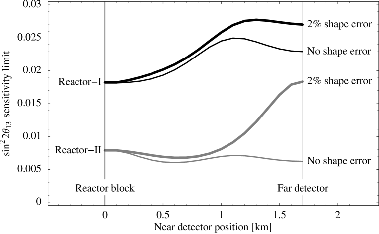
Figure 12: The sensitivity to $\sin^{2}2\theta_{13}$ at the $90\%$ confidence level for Reactor-I and Reactor-II as a function of the near detector position. The far detector is situated at 1.7 km and we assume identical detectors. Furthermore, the impact of an uncorrelated theoretical shape uncertainty of 2% is shown.

The results of this analysis are presented in Figure 12. We find that for the case of Reactor-I the limit starts deteriorating around a near detector distance of 400 m, whereas for Reactor-II the limit even improves slightly up to near detector baselines of $\sim 1\,\mathrm{km}$. Due to the high statistics in the case of Reactor-II, flux normalization and shape are very well determined by the near detector even in the presence of some effect of $\sin^{2}2\theta_{13}$, and the additional information on oscillations improves the limit a bit. Furthermore, we find from Figure 12 that the shape uncertainty becomes important for near detector baselines $\gtrsim 1.1\,\mathrm{km}$, especially for Reactor-II. A reduction of this theoretical error would be helpful in such a situation. We note that assuming the shape error to be completely uncorrelated corresponds to the worst case. A more realistic implementation of the shape uncertainty including correct correlations will lead to results somewhere in between the curves for no and 2% shape error in Figure 12. These calculations have been done for our standard value of $\Delta m_{31}^{2}=3\cdot 10^{-3}\,\mathrm{eV}^{2}$. However, we find very similar behavior for other values of $\Delta m_{31}^{2}$.

To summarize, for the case of Reactor-I-like experiments one should look for a site where the near detector can be placed at a distance of at most 400 m from the reactor. For large detectors, such as Reactor-II, near detector baselines of up to 1 km will perform well. For near detector baselines longer than about 1 km the correct treatment of the theoretical shape uncertainty becomes important.

References

- [1] Y. Fukuda et al. (Super-Kamiokande), Phys. Rev. Lett. 81, 1562 (1998), hep-ex/9807003
- [2] M. Ambrosio et al. (MACRO Collab.), Phys. Lett. B434, 451 (1998), hep-ex/9807005
- [3] F. Ronga, Nucl. Phys. Proc. Suppl. 100, 113 (2001)
- [4] M. Shiozawa (Super-Kamiokande) (2002), talk given at Neutrino 2002, Munich, Germany, http://neutrino2002.ph.tum.de
- [5] B. T. Cleveland et al., Astrophys. J. 496, 505 (1998)
- [6] J. N. Abdurashitov et al. (SAGE), J. Exp. Theor. Phys. 95, 181 (2002)
- [7] W. Hampel et al. (GALLEX), Phys. Lett. B447, 127 (1999)
- [8] M. Altmann et al. (GNO), Phys. Lett. B490, 16 (2000), hep-ex/0006034
- [9] S. Fukuda et al. (Super-Kamiokande), Phys. Lett. B539, 179 (2002), hep-ex/0205075
- [10] Q. R. Ahmad et al. (SNO), Phys. Rev. Lett. 89, 011301 (2002), nucl-ex/0204008
- [11] Q. R. Ahmad et al. (SNO), Phys. Rev. Lett. 89, 011302 (2002), nucl-ex/0204009
- [12] K. Eguchi et al. (KamLAND), Phys. Rev. Lett. 90, 021802 (2003), hep-ex/0212021
- [13] S. Pakvasa and J. W. F. Valle hep-ph/0301061
- [14] M. Apollonio et al. (Chooz Collab.), Phys. Lett. B466, 415 (1999), hep-ex/9907037
- [15] M. Apollonio et al. (2002), hep-ex/0301017
- [16] M. H. Ahn et al. (K2K), Phys. Rev. Lett. 90, 041801 (2003), hep-ex/0212007
- [17] V. Paolone, Nucl. Phys. Proc. Suppl. 100, 197 (2001)
- [18] D. Duchesneau (OPERA, 2002), hep-ex/0209082
- [19] P. Migliozzi and F. Terranova (2003), hep-ph/0302274
- [20] Y. Itow et al., Nucl. Phys. Proc. Suppl. 111, 146 (2001), hep-ex/0106019
- [21] D. Ayres et al. (2002), hep-ex/0210005
- [22] A. Asratyan et al., Science 124, 103 (2003), hep-ex/0303023
- [23] P. Huber, M. Lindner, and W. Winter, Nucl. Phys. B654, 3 (2003), hep-ph/0211300
- [24] K. Whisnant, J. M. Yang, and B.-L. Young (2002), hep-ph/0208193
- [25] H. Minakata and H. Nunokawa, JHEP 10, 001 (2001), hep-ph/0108085
- [26] V. Barger, S. Geer, R. Raja, and K. Whisnant, Phys. Rev. D63, 113011 (2001), arXiv:hep-ph/0012017
- [27] J. J. Gomez-Cadenas et al. (CERN working group on Super Beams), Nucl. Phys. B646, 321 (2001), hep-ph/0105297
- [28] M. Aoki et al. (2001), hep-ph/0112338
- [29] M. Aoki (2002), hep-ph/0204008
- [30] G. Barenboim, A. De Gouvea, M. Szleper, and M. Velasco, Nucl. Phys. B631, 239 (2002), hep-ph/0204208
- [31] M. Aoki, K. Hagiwara, and N. Okamura, Phys. Rev. D54, 3667 (2002), hep-ph/0208223
- [32] G. Barenboim and A. de Gouvea (2002), hep-ph/0209117
- [33] N. Okamura, Phys. Rev. D34, 2621 (2002), hep-ph/0209123
- [34] M. Mezzetto (2003), hep-ex/0302005
- [35] M. V. Diwan et al. (2003), hep-ph/0303081
- [36] M. Apollonio et al. (2002), hep-ph/0210192
- [37] G. L. Fogli and E. Lisi, Phys. Rev. D54, 3667 (1996), hep-ph/9604415
- [38] J. Burguet-Castell, M. B. Gavela, J. J. Gomez-Cadenas, P. Hernandez, and O. Mena, Nucl. Phys. B608, 301 (2001), hep-ph/0103258
- [39] V. Barger, D. Marfatia, and K. Whisnant, Phys. Rev. D65, 073023 (2002), hep-ph/0112119
- [40] P. Huber, M. Lindner, and W. Winter, Nucl. Phys. B645, 3 (2002), hep-ph/0204352
- [41] V. Barger, D. Marfatia, and K. Whisnant, Phys. Rev. D66, 053007 (2002), hep-ph/0206038
- [42] P. Huber and W. Winter (2003), hep-ph/0301257
- [43] J. Burguet-Castell, M. B. Gavela, J. J. Gomez-Cadenas, P. Hernandez, and O. Mena, Nucl. Phys. B646, 301 (2002), hep-ph/0207080
- [44] H. Minakata, H. Nunokawa, and S. Parke (2002), hep-ph/0208163
- [45] V. Barger, D. Marfatia, and K. Whisnant (2002), hep-ph/0210428
- [46] H. Minakata, H. Nunokawa, and S. Parke (2003), hep-ph/0301210
- [47] L. A. Mikaelyan and V. V. Sinev, Phys. Atom. Nucl. 63, 1002 (2000), hep-ex/9908047
- [48] L. Mikaelyan, Nucl. Phys. Proc. Suppl. 91, 120 (2001), hep-ex/0008046
- [49] L. A. Mikaelyan, Phys. Atom. Nucl. 65, 1173 (2002), hep-ph/0210047
- [50] V. Martemyanov, L. Mikaelyan, V. Sinev, V. Kopeikin, and Y. Kozlov (2002), hep-ex/0211070
- [51] H. Minakata, H. Sugiyama, O. Yasuda, K. Inoue, and F. Suekane (2002), hep-ph/0211111
- [52] M. Shaevitz (2003), talk given at NOON 2003, Kanazawa, Japan, http://www-sk.icrr.u-tokyo.ac.jp/noon2003/
- [53] C. L. Cowan, F. Reines, F. B. Harrison, H. W. Kruse, and A. D. McGuire, Science 124, 103 (1956)
- [54] G. Zacek et al. (CALTECH-SIN-TUM), Phys. Rev. D34, 2621 (1986)
- [55] Y. Declais et al., Nucl. Phys. B434, 503 (1995)
- [56] F. Boehm et al., Phys. Rev. D64, 112001 (2001), hep-ex/0107009
- [57] C. Bemporad, G. Gratta, and P. Vogel, Rev. Mod. Phys. 74, 297 (2002), hep-ph/0107277
-
[58]
Particle Data Group, D.E. Groom et al.,
Eur. Phys. J. C 15,
1 (2000),
http://pdg.lbl.gov/ - [59] M. Freund, P. Huber, and M. Lindner, Nucl. Phys. B615, 331 (2001), hep-ph/0105071
- [60] A. Cervera et al., Nucl. Phys. B579, 17 (2000), erratum ibid. Nucl. Phys. B593, 731 (2001), hep-ph/0002108
- [61] M. Freund, Phys. Rev. D64, 053003 (2001), hep-ph/0103300
- [62] M. Freund, M. Lindner, S. T. Petcov, and A. Romanino, Nucl. Phys. B578, 27 (2000), hep-ph/9912457
- [63] M. C. Gonzalez-Garcia and M. Maltoni, Eur. Phys. J. C26, 417 (2003), hep-ph/0202218
- [64] M. Maltoni, T. Schwetz, M. A. Tortola, and J. W. F. Valle, Phys. Rev. D67, 013011 (2003), hep-ph/0207227
- [65] G. L. Fogli, E. Lisi, A. Marrone, and D. Montanino hep-ph/0303064
- [66] M. Maltoni, T. Schwetz, and J. W. F. Valle (2002), hep-ph/0212129
- [67] J. N. Bahcall, M. C. Gonzalez-Garcia, and C. Pena-Garay, JHEP 02, 009 (2003), hep-ph/0212147
- [68] G. L. Fogli et al., JHEP 02, 009 (2003), hep-ph/0212127
- [69] P. C. de Holanda and A. Y. Smirnov (2002), hep-ph/0212270
- [70] A. Bandyopadhyay, S. Choubey, R. Gandhi, S. Goswami, and D. P. Roy (2002), hep-ph/0212146
-
[71]
V. Barger,
D. Marfatia, and
B. Wood,
Phys. Lett. B498,
53 (2001),
hep-ph/0011251 - [72] A. de Gouvea and C. Pena-Garay, Phys. Rev. D64, 113011 (2001), hep-ph/0107186
- [73] M. C. Gonzalez-Garcia and C. Pea-Garay, Phys. Lett. B527, 199 (2002), hep-ph/0111432
- [74] R. J. Geller and T. Hara, Phys. Rev. Lett. 49, 98 (2001), hep-ph/0111342
- [75] P. Vogel and J. F. Beacom, Phys. Rev. D60, 053003 (1999), hep-ph/9903554
- [76] P. Vogel and J. Engel, Phys. Rev. D39, 3378 (1989)
- [77] H. Murayama and A. Pierce, Phys. Rev. D65, 013012 (2002), hep-ph/0012075
- [78] G. Alimonti et al., Nucl. Instrum. Meth. A406, 411 (1998)
- [79] S. Schonert, T. Lasserre, and L. Oberauer, Astropart. Phys. 18, 565 (2003), hep-ex/0203013
- [80] L. Oberauer, private communication
- [81] D. Beavis et al., Proposal of BNL AGS E-889, Tech. Rep., BNL (1995)
- [82] S. T. Petcov and M. Piai, Phys. Lett. B533, 94 (2002), hep-ph/0112074.