YUKAWA QUASI-UNIFICATION
AND NEUTRALINO RELIC DENSITY
Invited talk at the EUnet “Supersymmetry and the Early Universe”
mid-term meeting, Oxford, 26-29 September 2002

Abstract

The construction of a Supersymmetric Grand Unified Model based on the Pati-Salam gauge group is briefly reviewed and the low energy consequences of the derived asymptotic Yukawa quasi-unification conditions are examined. In the framework of the resulting Constrained Minimal Supersymmetric Standard Model, the cosmological relic density of the bino-like LSP is calculated and the results are explicitly compared with micrOMEGAs. In addition to the Cold Dark Matter constraint, restrictions on the parameter space, arising from the Higgs boson masses, the SUSY corrections to $b$-quark mass, the muon anomalous magnetic moment and the inclusive decay $b\rightarrow s\gamma$ are, also, investigated. For $\mu>0$, a wide and natural range of parameters is allowed. On the contrary, the $\mu<0$ case not only is disfavored from the present experimental data on the muon anomalous magnetic moment, but also, it can be excluded from the combination of the Cold Dark Matter and BR($b\rightarrow s\gamma$) requirements.

1 INTRODUCTION

This review is based on Refs. [1]. We briefly describe a Supersymmetric (SUSY) Grand Unified Theory (GUT) which predicts a set of asymptotic Yukawa quasi-unification conditions (YQUCs) in sec. 2 and then we show how we can restrict the parameter space of the resulting Constrained Minimal Supersymmetric Standard Model (CMSSM) using a number of Cosmo-Phenomenological requirements (sec. 3-4). Particular emphasis will be given in the Neutralino Relic Density calculation in sec. 3. Some conclusions and open issues will close this presentation in sec. 5.

2 YUKAWA QUASI-UNIFICATION

The motivation of our construction is given in subsec. 2.1 and a brief description of the model building follows in subsec. 2.2. Finally, in subsec. 2.3, the mass parameters of the resulting CMSSM versions are derived.

2.1 THE YUKAWA UNIFICATION HYPOTHESIS

We focus on a SUSY GUT based on the Pati Salam (PS) gauge group $(SU(4)_{\rm c}\otimes SU(2)_{L}$ $\otimes SU(2)_{R}={\bf 4}_{\rm c}{\bf 2}_{L}{\bf 2}_{R})$ described in detail in Ref. [2]. The relevant field content of the Model is presented in the Table 1, where the components, the representations, the transformations and the extra global charges of the various superfields are, also, shown. The left handed quarks and leptons superfields of every generation $r$ are accommodated in a single pair of superfields $F_{r},F^{c}_{r}$. The PS symmetry can be spontaneously broken down to Standard Model (SM) one through the vacuum expectation values (vevs) which the superfields $H^{c},\bar{H}^{c}$ acquire in the direction of the right handed neutrinos, $\nu^{c}_{H},\bar{\nu}^{c}_{H}$.

In the simplest realization of this model, as it is proposed by Antoniadis and Leontaris in Ref. [3], the electroweak doublets $H_{1},H_{2}$ are exclusively contained in the bidoublet superfield $h$, which can be written:

$$h=\left\lgroup\matrix{h_{2}&h_{1}}\right\rgroup,\>\>\mbox{with}\>\>h_{1}=\left\lgroup\matrix{h^{0}_{1}\cr h^{-}_{1}}\right\rgroup\>\>\mbox{and}\>\>h_{2}=\left\lgroup\matrix{h^{+}_{2}\cr h^{0}_{2}}\right\rgroup\cdot$$ (1)

With these assumptions, the model predicts Yukawa unification (YU) at GUT scale, $M_{\rm GUT}$ ($M_{\rm GUT}$ is determined by the requirement of gauge coupling unification):

$$h_{t}(M_{\rm GUT})=h_{b}(M_{\rm GUT})=h_{\tau}(M_{\rm GUT})=y_{33},$$ (2)

since the Yukawa coupling terms of the resulting version of MSSM originate from a unique term of the underlying GUT, as follows:

$$y_{33}\>F_{3}\>h\>F_{3}^{c}\>\>\ni\>\>y_{33}\>(H_{2}^{\mbox{\sf\scriptsize T}}i\tau_{2}Q\;t^{c}+H_{1}^{\mbox{\sf\scriptsize T}}i\tau_{2}Q\;b^{c}+H_{1}^{\mbox{\sf\scriptsize T}}i\tau_{2}L\;\tau^{c}),~{}~{}\mbox{since}~{}~{}H_{1[2]}=h_{1[2]}.$$ (3)

Here $Q,L\ni-i\tau_{2}F_{3}^{\mbox{\sf\scriptsize T}}$ are the well known $SU(2)_{L}$ doublets quarks and leptons of the third family and the self explanatory substitutions $(t,b,\tau)$ in the position of $(u_{3},d_{3},e_{3})$ appeared in the Table 1 are made. Also, $\tau_{2}$ is the second Pauli matrix, $\ni$ means “belongs to” and the brackets are used by applying disjunctive correspondence.

However, applying this scheme in the context of the CMSSM [4] and given the top and tau experimental masses (which naturally restrict the $\tan\beta\simeq 50$), the pre-diction of the (asymptotic) YU leads to a contra-diction with the experimental bounds on $b$-quark mass. This is due to the fact that in the large $\tan\beta$ regime, the tree level $b$-quark mass, $m_{b}$, receives sizeable (about 20$\%$) SUSY corrections [5] $\Delta m_{b}(M_{\rm SUSY})$, evaluated at a SUSY breaking scale $M_{\rm SUSY}$ (see sec. 2.3). These corrections arise from sbottom-gluino (mainly) and stop-chargino loops [5, 6, 7] and have the sign of $\mu$ (with the standard sign convention of Ref. [8]). Their size is a 1-loop exact quantity, as it is explained in Ref. [7]. Hence, for $\mu>[<]~{}0$, the SUSY corrections drive the corrected (which is essentially the so called running [7]) $b$-quark mass, $m^{\rm c}_{b}$, at a low scale $M_{Z}$,

$$m^{\rm c}_{b}(M_{Z})=m_{b}(M_{Z})\Big{(}1+\Delta m_{b}(M_{\rm SUSY})\Big{)}$$ (4)

a lot above [a little below] than its $95\%$ confidence level (c.l.) experimental range. This is derived by appropriately [1] evolving the corresponding range for the pole $b$-quark mass, $m_{b}(m_{b})$ up to $M_{Z}$ scale with $\alpha_{s}(M_{Z})\simeq 0.1185$, in accord with the analysis in Ref. [9]:

$$m_{b}(m_{b})=4.25\pm 0.3\>{\rm GeV}\>\>\>\stackrel{{\scriptstyle}}{{\Longrightarrow}}\>\>\>m^{\rm c}_{b}(M_{Z})=2.88\pm 0.2\>{\rm GeV}$$ (5)

Concluding, for both signs of $\mu$ the YU assumption leads to an unacceptable $b$-quark mass. The discrepancy is less sizable for $\mu<0$, so we can say that YU “prefers” [10] $\mu<0$.

The usual strategy to accommodate the latter discrepancy is the introduction of several kinds of nonuniversalities in the scalar [11, 12, 13] and/or gaugino [10] sector of MSSM, without an exact conservation of the YU. On the contrary, in Ref. [1], this problem is addressed in the context of the PS GUT, without need of invoking the departure from the CMSSM [4] universality. The Higgs sector of the model is extended so, that the electroweak Higgs in Eq. (3) receive subdominant contributions from other representations, too. As a consequence, a moderate violation of the YU is obtained, which can allow an acceptable $b$-quark mass, even with universal boundary conditions.

Table 1: RELEVANT FIELD CONTENT

FIELDS	COMPONENTS	REPRESE-	TRASFOR-	GLOBAL
		NTATIONS	MATIONS	SYMMETRIES
(Color Index Suppressed)		${\bf 4}_{\rm c}{\bf 2}_{L}{\bf 2}_{R}$		$R$	$PQ$	$Z^{mp}_{2}$
MATTER FIELDS
$F_{r}$	$\matrix{\left\lgroup\matrix{d_{r}&-u_{r}}\right\rgroup\cr\left\lgroup\matrix{e_{r}&-\nu_{r}}\right\rgroup}$	$({\bf 4,2,1})$	$F_{r}U_{L}^{\dagger}U^{\mbox{\sf\scriptsize T}}_{\rm c}$	$1/2$	$-1$	$1$
$F^{c}_{r}$	$\mbox{ $\left\lgroup\matrix{u^{c}_{r}\cr d^{c}_{r}}\right\rgroup$},\mbox{ $\left\lgroup\matrix{\nu^{c}_{r}\cr e^{c}_{r}}\right\rgroup$}$	$({\bf\bar{4},1,2})$	$U_{\rm c}^{\ast}U_{R}^{\ast}F^{c}_{r}$	$1/2$	$0$	$-1$
($r=1,2,3$: Generation Index)
HIGGS FIELDS
$H^{c}$	$\mbox{ $\left\lgroup\matrix{u^{c}_{H}\cr d^{c}_{H}}\right\rgroup$},\mbox{ $\left\lgroup\matrix{\nu^{c}_{H}\cr e^{c}_{H}}\right\rgroup$}$	$({\bf\bar{4},1,2})$	$U_{\rm c}^{\ast}U_{R}^{\ast}H^{c}$	$0$	$0$	$0$
$\bar{H}^{c}$	$\matrix{\left\lgroup\matrix{\bar{u}^{c}_{H}&\bar{d}^{c}_{H}}\right\rgroup\cr\left\lgroup\matrix{\bar{\nu}^{c}_{H}&\bar{e}^{c}_{H}}\right\rgroup}$	$({\bf 4,1,2})$	$\bar{H}^{c}U^{\mbox{\sf\scriptsize T}}_{R}U^{\mbox{\sf\scriptsize T}}_{\rm c}$	$0$	$0$	$0$
$h$	$\left\lgroup\matrix{h^{+}_{2}&h^{0}_{1}\cr h^{0}_{2}&h^{-}_{1}}\right\rgroup$	$({\bf 1,2,2})$	$U_{L}hU^{\mbox{\sf\scriptsize T}}_{R}$	$0$	$1$	$0$
EXTRA HIGGS FIELDS
$h^{\prime}$	$\left\lgroup\matrix{h^{\prime+}_{2}&h^{\prime 0}_{1}\cr h^{\prime 0}_{2}&h^{\prime-}_{1}}\right\rgroup$	$({\bf 15,2,2})$	$U_{\rm c}^{\ast}U_{L}h^{\prime}U^{\mbox{\sf\scriptsize T}}_{R}U^{\mbox{\sf\scriptsize T}}_{\rm c}$	$0$	$1$	$0$
$\bar{h}^{\prime}$	$\left\lgroup\matrix{\bar{h}^{\prime+}_{2}&\bar{h}^{\prime 0}_{1}\cr\bar{h}^{\prime 0}_{2}&\bar{h}^{\prime-}_{1}}\right\rgroup$	$({\bf 15,2,2})$	$U_{\rm c}U_{L}\bar{h}^{\prime}U^{\mbox{\sf\scriptsize T}}_{R}U_{\rm c}^{\dagger}$	$1$	$-1$	$0$
$\phi$	$\mbox{ $\left\lgroup\matrix{\phi&0\cr 0&-\phi}\right\rgroup$ }^{(\ast)}$	$({\bf 15,1,3})$	$U_{\rm c}U_{R}\phi U_{R}^{\dagger}U_{\rm c}^{\dagger}$	$0$	$0$	$0$
$\bar{\phi}$	$\mbox{ $\left\lgroup\matrix{\bar{\phi}&0\cr 0&-\bar{\phi}}\right\rgroup$ }^{(\ast)}$	$({\bf 15,1,3})$	$U_{\rm c}U_{R}\bar{\phi}U_{R}^{\dagger}U_{\rm c}^{\dagger}$	$1$	$0$	$0$
			$U_{\rm c}\in SU(4)_{\rm c}$
	(∗)SM neutral		$U_{L}\in SU(2)_{L}$
	content		$U_{R}\in SU(2)_{R}$

2.2 MODEL CONSTRUCTION

From the discussion of the previous section, we can induce that a small deviation from the YU will be enough for an appropriate prediction of $b$-quark mass when $\mu<0$, while for $\mu>0$, a more pronounced deviation is needed. According to the first paper in Ref. [1], this can be achieved by introducing some extra higgs fields, as follows:

Since the matter fields product has the following structure under ${\bf 4}_{\rm c}{\bf 2}_{L}{\bf 2}_{R}$:

$$F_{3}F_{3}^{c}\ni{\bf(4,2,1)}\otimes{\bf(\bar{4},1,2)}={\bf(1,2,2)}\oplus{\bf(15,2,2)}$$ (6)

and ${\bf 15}_{SU(4)}\ni{\bf 1}_{SU(3)}$, it is possible the addition of two higgs superfields:

$$h^{\prime},\>\bar{h}^{\prime}\>\>\in\>\>{\bf(15,2,2)}.$$ (7)

The field $h^{\prime}$ can couple to $F_{3}F_{3}^{c}$ and $\bar{h}^{\prime}$ can give mass to the color non singlets through a mixing term $m\bar{h}^{\prime}h^{\prime}$ with $m\sim M_{\rm GUT}\simeq 2\times 10^{16}~{}{\rm GeV}$, in accord with the imposed global symmetries (see Table 1). Other possible mixing term suppressed by the string scale $M_{S}\simeq 5\times 10^{17}~{}{\rm GeV}$, being non renormalizable, is:

$$\bar{H}^{c}H^{c}\bar{h}^{\prime}h/M_{S}\>\>\ni\>\>\Big{(}{\bf 15}\otimes{\bf 15},~{}{\bf 1}\otimes{\bf 1},~{}({\bf 1}\oplus{\bf 3})\otimes({\bf 1}\oplus{\bf 3})\Big{)},$$ (8)

with the latter structure under ${\bf 4}_{\rm c}{\bf 2}_{L}{\bf 2}_{R}$, since for the 2 participants of the product, we get:

$$\bar{H}^{c}H^{c}~{}[\bar{h}^{\prime}h]~{}~{}\in~{}~{}\Big{(}{\bf 15}\oplus{\bf 1}~{}[{\bf 15}],~{}{\bf 1}~{}[{\bf 1}\oplus{\bf 3}],~{}{\bf 1}\oplus{\bf 3}\Big{)}.$$

In the term of Eq. (8), there are 2 couplings as regards the $SU(2)_{R}$: A singlet, $\lambda_{\bf 1}(\bar{H}^{c}H^{c})_{\bf 1}$ $\bar{h}^{\prime}h$ (since ${\bf 1}\otimes{\bf 1}={\bf 1}$), and a triplet, $\lambda_{\bf 3}(\bar{H}^{c}H^{c})_{\bf 3}\bar{h}^{\prime}h$ (since ${\bf 3}\otimes{\bf 3}={\bf 1}\oplus{\bf 3}\oplus{\bf 5}$). As it turns out, the singlet coupling provides us with an adequate deviation from the YU for $\mu<0$. The necessary deviation for $\mu>0$ can be obtained by a further enlargement of the Higgs sector, such that contributions arising from renormalizable terms are allowed. By introducing two additional Higgs fields:

$$\phi,\>\bar{\phi}\>\>\in\>\>{\bf(15,1,3)}$$ (9)

an unsuppressed coupling $\lambda^{\prime}_{\bf 3}\phi\bar{h}^{\prime}h$ (again since ${\bf 3}\otimes{\bf 3}={\bf 1}\oplus{\bf 3}\oplus{\bf 5}$) can be constructed. This overshadows the coupling $\lambda_{\bf 3}(\bar{H}^{c}H^{c})_{\bf 3}\bar{h}^{\prime}h$. $\bar{\phi}$ is introduced to give superheavy masses to the color non singlets in $\phi$ through a term $\bar{\phi}\phi$. Summarizing, the important mixing terms are:

$$m\bar{h}^{\prime}h^{\prime},\>\lambda_{{\bf 1}[{\bf 3}]}(\bar{H}^{c}H^{c})_{{\bf 1}[{\bf 3}]}\bar{h}^{\prime}h/M_{S}~{}~{}\mbox{and}~{}~{}\lambda^{\prime}_{\bf 3}\phi\bar{h}^{\prime}h~{}~{}\left(\lambda_{{\bf 1}[{\bf 3}]},\lambda^{\prime}_{\bf 3}:~{}\mbox{dimensionless constants}\right).$$

Using the transformation properties of the several fields indicated in the Table 1, and taking into account the unitarity of the $SU(2)_{L,R}$ groups, we conclude that the previous mixing terms correspond to the following invariant quantities under ${\bf 4}_{\rm c}{\bf 2}_{L}{\bf 2}_{R}$, respectively:

$$m\mbox{\sf Tr}\left(\bar{h}^{\prime}i\tau_{2}h^{\prime{\mbox{\sf\scriptsize T}}}i\tau_{2}\right),\>\>\frac{\lambda_{{\bf 1}[{\bf 3}]}}{M_{S}}\mbox{\sf Tr}\left(\bar{h}^{\prime}i\tau_{2}(\bar{H}^{c{\mbox{\sf\scriptsize T}}}H^{c{\mbox{\sf\scriptsize T}}})_{{\bf 1}[{\bf 3}]}h^{\mbox{\sf\scriptsize T}}i\tau_{2}\right)\>\>\mbox{and}\>\>\lambda^{\prime}_{\bf 3}\mbox{\sf Tr}\left(\bar{h}^{\prime}i\tau_{2}\phi h^{\mbox{\sf\scriptsize T}}i\tau_{2}\right),$$ (10)

where the traces are taken with respect to the $SU(4)_{\rm c}$ and $SU(2)_{L}$ indices.

At GUT scale, during the spontaneous breaking of PS gauge symmetry, the fields $\bar{H}^{c},H^{c}$ and $\phi$ acquire vevs in the SM singlet direction. Therefore,

$$\left(\langle\bar{H}^{c{\mbox{\sf\scriptsize T}}}\rangle\langle H^{c{\mbox{\sf\scriptsize T}}}\rangle\right)_{{\bf 1}[{\bf 3}]}=v^{2}_{H^{c}}\left(T_{H^{c}},1,\frac{\sigma_{0[3]}}{2}\right)\>\>\mbox{and}\>\>\langle\phi\rangle=v_{\phi}\left(T^{15},1,\frac{\sigma_{3}}{\sqrt{2}}\right),$$ (11)

where $v_{H^{c},\phi}\sim M_{\rm GUT}$ and the three-fold structure of these vevs as regards the ${\bf 4}_{\rm c}{\bf 2}_{L}{\bf 2}_{R}$ group is ordered in the parenthesis by commas, with

$$T_{H^{c}}={\sf diag}\Big{(}0,0,0,1\Big{)},~{}~{}T^{15}=\frac{1}{2\sqrt{3}}\>{\sf diag}\Big{(}1,1,1,-3\Big{)}~{}~{}\mbox{and}~{}~{}\sigma_{0[3]}={\sf diag}\Big{(}1,[-]1\Big{)}.$$ (12)

Expanding the superfields in Eq. (7) as linear combination of the 15 generators $T^{a}$ of $SU(4)_{\rm c}$ with the normalization $\mbox{\sf Tr}(T^{a}T^{b})=\delta^{ab}$ and denoting the SM singlet components with the superfield symbol, the following identities can be easily proved:

$$\mbox{\sf Tr}\left(\bar{h}^{\prime}i\tau_{2}h^{\prime{\mbox{\sf\scriptsize T}}}i\tau_{2}\right)=\bar{h}^{\prime{\mbox{\sf\scriptsize T}}}_{1}i\tau_{2}h^{\prime}_{2}+h^{\prime{\mbox{\sf\scriptsize T}}}_{1}i\tau_{2}\bar{h}^{\prime}_{2}+{\cal O}(T^{a}T^{a},~{}a<15),$$ (13)

$$\mbox{\sf Tr}\left(\bar{h}^{\prime}i\tau_{2}\left(T^{15}_{[H^{c}]},1,\sigma_{3[0]}\right)h^{\mbox{\sf\scriptsize T}}i\tau_{2}\right)=\left(\bar{h}^{\prime{\mbox{\sf\scriptsize T}}}_{1}i\tau_{2}h_{2}-[+]h^{\mbox{\sf\scriptsize T}}_{1}i\tau_{2}\bar{h}^{\prime}_{2}\right)\left[-\sqrt{3}/2\right],$$ (14)

where the notation of Eqs. (11) was applied. Inserting Eqs. (11) in Eqs. (10) and employing Eqs. (13)-(14), we get the mass terms:

$$m\bar{h}^{\prime{\mbox{\sf\scriptsize T}}}_{1}i\tau_{2}\left(h^{\prime}_{2}+\alpha_{2}h_{2}\right)+m\left(h^{\prime{\mbox{\sf\scriptsize T}}}_{1}+\alpha_{1}h^{\mbox{\sf\scriptsize T}}_{1}\right)i\tau_{2}\bar{h}^{\prime}_{2},$$ (15)

where the the mixing effects are included in the following coefficients:

$$\alpha_{1[2]}=\frac{1}{\sqrt{2}m}\left(-[+]\,\left(\lambda^{\prime}_{\bf 3}v_{\phi}-\frac{\sqrt{6}}{4M_{S}}\lambda_{\bf 3}v^{2}_{H^{c}}\right)-\frac{\sqrt{6}}{4M_{S}}\lambda_{\bf 1}v^{2}_{H^{c}}\right)\cdot$$ (16)

It is obvious from Eq. (15) that we obtain 2 combinations of superheavy massive fields:

$$\bar{h}^{\prime}_{1},~{}H^{\prime}_{1}~{}~{}\mbox{and}~{}~{}\bar{h}^{\prime}_{2},~{}H^{\prime}_{2},~{}~{}\mbox{where}~{}~{}H^{\prime}_{i}=\frac{h^{\prime}_{i}+\alpha_{i}h_{i}}{\sqrt{1+|\alpha_{i}|^{2}}},~{}i=1,2.$$ (17)

The electroweak doublets, remaining massless at GUT scale, can be interpreted as “orthogonal” to $H^{\prime}_{i}$ direction:

$$H_{i}=\frac{-\alpha_{i}^{*}h^{\prime}_{i}+h_{i}}{\sqrt{1+|\alpha_{i}|^{2}}}$$ (18)

Solving Eqs. (18) and (17) as respect $h_{i}$ and $h^{\prime}_{i}$, we obtain:

$$h_{i}=\frac{H_{i}+\alpha^{*}_{i}H^{\prime}_{i}}{\sqrt{1+|\alpha_{i}|^{2}}}~{}~{}\mbox{and}~{}~{}h^{\prime}_{i}=\frac{-\alpha_{i}H_{i}+H^{\prime}_{i}}{\sqrt{1+|\alpha_{i}|^{2}}}\cdot~{}~{}~{}$$ (19)

Consequently, the Yukawa couplings terms, in contrast to Eq. (3), take the form:

$$y_{33}\>F_{3}\>h\>F_{3}^{c}+2y^{\prime}_{33}\>F_{3}\>h^{\prime}\>F_{3}^{c}\>\>\ni\>\>y_{33}\>F_{3}\left\lgroup\matrix{h_{2}+2\rho T^{15}h^{\prime}_{2}&h_{1}+2\rho T^{15}h^{\prime}_{1}}\right\rgroup F_{3}^{c}\>\>\ni$$

$$y_{33}\>\left(\frac{1-\rho\alpha_{2}/\sqrt{3}}{\sqrt{1+|\alpha_{2}|^{2}}}\>H_{2}^{\mbox{\sf\scriptsize T}}i\tau_{2}Q\>t^{c}+\frac{1-\rho\alpha_{1}/\sqrt{3}}{\sqrt{1+|\alpha_{1}|^{2}}}\>H_{1}^{\mbox{\sf\scriptsize T}}i\tau_{2}Q\>b^{c}+\frac{1+\sqrt{3}\rho\alpha_{1}}{\sqrt{1+|\alpha_{1}|^{2}}}\>H_{1}^{\mbox{\sf\scriptsize T}}i\tau_{2}L\>\tau^{c}\right),$$

where $\rho=y^{\prime}_{33}/y_{33}$ with $0<\rho<1$ and only color singlets components of $h^{\prime}_{i}$ are shown. The fields $H^{\prime}_{i}$ being superheavy mass states, contribute neither to the running of renormalization group equations (RGEs) nor to the masses of fermions. Consequently, the asymptotic exact YU in Eq. (2) can be replaced by a set of asymptotic YQUCs:

$$h_{t}(M_{\rm GUT}):h_{b}(M_{\rm GUT}):h_{\tau}(M_{\rm GUT})=\left|\frac{1-\rho\alpha_{2}/\sqrt{3}}{\sqrt{1+|\alpha_{2}|^{2}}}\right|:\left|\frac{1-\rho\alpha_{1}/\sqrt{3}}{\sqrt{1+|\alpha_{1}|^{2}}}\right|:\left|\frac{1+\sqrt{3}\rho\alpha_{1}}{\sqrt{1+|\alpha_{1}|^{2}}}\right|\cdot~{}~{}~{}~{}$$ (20)

The deviation from the YU can be estimated, by defining the following relative splittings:

$$\delta h_{b[\tau]}=\left(h_{b[\tau]}(M_{\rm GUT})-h_{t}(M_{\rm GUT})\right)/h_{t}(M_{\rm GUT}).$$ (21)

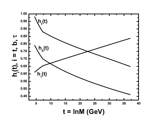
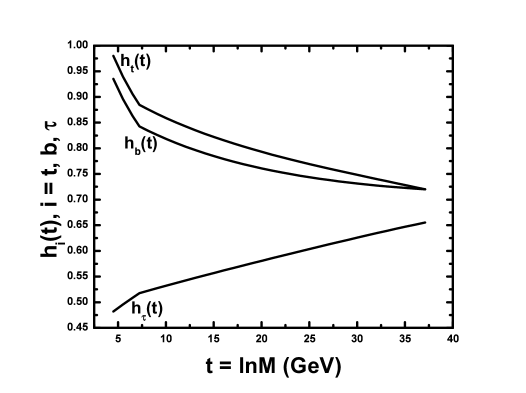
Figure 1: A Yukawa couplings running from $M_{\rm GUT}$ to $M_{Z}$ for $m^{\rm c}_{b}(M_{Z})=2.68~{}{\rm GeV}$, $\mu>[<]~{}0$, $m_{\rm LSP}=297~{}[372]~{}{\rm GeV}$ and $\Delta_{\tilde{\tau}_{2}}=1.5~{}[0]$ corresponding to $\tan\beta\simeq 59~{}[50]$ (left [right] plot).

2.3 CMSSM WITH YUKAWA QUASI-UNIFICATION

Below the $M_{\rm GUT}$, our particle content reduces to this of MSSM. We assume universal soft SUSY breaking scalar masses, $m_{0}$, gaugino masses, $M_{1/2}$ and trilinear scalar couplings, $A_{0}$ at $M_{\rm GUT}$. Therefore, the resulting MSSM is the so called CMSSM [4] supplemented by a suitable YQUC from the set in Eq. (20). With these initial conditions, we run the MSSM RGEs [14] between $M_{\rm GUT}$ and a common SUSY threshold $M_{\rm SUSY}\simeq(m_{\tilde{t}_{1}}m_{\tilde{t}_{2}})^{1/2}$ ($\tilde{t}_{1,2}$ are the stop mass eigenstates) determined in consistency with the SUSY spectrum. At $M_{\rm SUSY}$ we impose radiative electroweak symmetry breaking, evaluate the SUSY spectrum and incorporate the SUSY corrections to $b$ and $\tau$ masses [6, 7, 11]. The latter (almost 4$\%$) lead [14] to a small de[in]-crease of $\tan\beta$ for $\mu>[<]~{}0$. From $M_{\rm SUSY}$ to $M_{Z}$, the running of gauge and Yukawa couplings is continued using the SM RGEs.

For presentation purposes, $M_{1/2}$ and $m_{0}$ can be replaced [14] by the lightest SUSY particle (LSP) mass, $m_{\rm LSP}$ and the relative mass splitting between it and the lightest stau $\tilde{\tau}_{2}$, $\Delta_{\tilde{\tau}_{2}}$. For simplicity, we restrict this presentation to the $A_{0}=0$ case (for $A_{0}\neq 0$ see Refs. [1, 15]). Our parameter “transmutation” is shown schematically, as follows:

$${\rm sign}\mu,\>M_{1/2},\ m_{0},\ A_{0}\>\>\stackrel{{\scriptstyle A_{0}=0}}{{\Longrightarrow}}\>\>{\rm sign}\mu,\>m_{\rm LSP},\ \Delta_{\tilde{\tau}_{2}}\>\>\>\left(\Delta_{\tilde{\tau}_{2}}=(m_{\tilde{\tau}_{2}}-m_{\rm LSP})/m_{\rm LSP}\right)$$

We restrict ourselves to monoparametric YQUCs derived from the general Eq. (20) with real $\alpha_{1,2}$. It is convenient to define the quantity:

$$c=\rho\alpha_{1}/\sqrt{3}~{}~{}\mbox{with}~{}~{}-1/3<c<1$$

For any given $m^{\rm c}_{b}(M_{Z})$ in Eq. (5) with fixed top, $m_{t}(m_{t})=166~{}{\rm GeV}$ and tau, $m^{\rm c}_{\tau}(M_{Z})=1.746~{}{\rm GeV}$ masses, we can determine the parameters $c$ and $\tan\beta$ at $M_{\rm SUSY}$ so, that the YQUC in Eq. (20) is satisfied. However, for the plots in Figs. 1, 2 and 3 we fix $m^{\rm c}_{b}(M_{Z})=2.68~{}{\rm GeV}$, since this value turns out to overlap the allowed areas for $\mu>0$ or give the less restrictive upper bound for $\mu<0$ on the $m_{\rm LSP}-\Delta_{\tilde{\tau}_{2}}$ plane (Figs. 4 and 5).

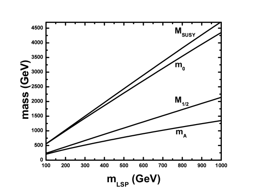
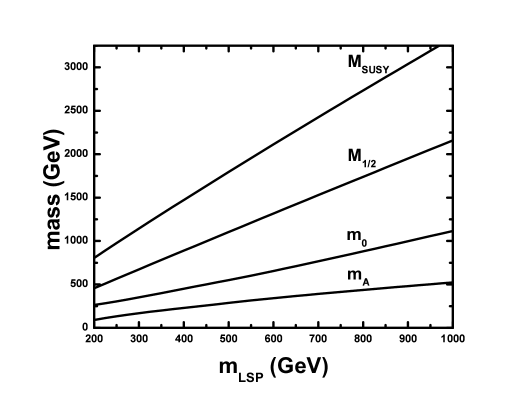
Figure 2: The mass parameters $m_{A}$, $m_{0}$, $M_{1/2}$ and $M_{\rm SUSY}$ versus $m_{\rm LSP}$ for $m^{\rm c}_{b}(M_{Z})=2.68~{}{\rm GeV}$, $\mu>[<]~{}0$ and $\Delta_{\tilde{\tau}_{2}}=1.5~{}[0]$ corresponding to $\tan\beta\simeq 59~{}[50]$ (left [right] plot).

The YQUC predicting appropriate values for $m^{\rm c}_{b}(M_{Z})$ relates the minimal Higgs content of the model described in sec. 2.2 to the sign of $\mu$, as follows:

$\bullet$ For $\mu>0$ the fields of Eq. (9) are needed. Viable CMSSM spectrum is obtained for $\alpha_{1}=-\alpha_{2}\>\sim\>1$ in Eq. (16). Therefore, Eq. (20) implies:

$$h_{t}(M_{\rm GUT}):h_{b}(M_{\rm GUT}):h_{\tau}(M_{\rm GUT})=|1+c|:|1-c|:|1+3c|.$$ (22)

In the left panel of Fig. 1, we present a typical Yukawa couplings running from $M_{\rm GUT}$ to $M_{Z}$ for $m_{\rm LSP}=297~{}{\rm GeV}$ and $\Delta_{\tilde{\tau}_{2}}=1.5$. In the left panel of Fig. 2, the values of $m_{A}$, $m_{0}$, $M_{1/2}$ and $M_{\rm SUSY}$ versus $m_{\rm LSP}$ are, also, displayed for the same $\Delta_{\tilde{\tau}_{2}}$. We observe that $M_{1/2}<m_{0}$ and $2m_{\rm LSP}\simeq m_{A}$ for $m_{\rm LSP}<350~{}{\rm GeV}$. For $2.68~{}{\rm GeV}\lesssim m^{\rm c}_{b}(M_{Z})\lesssim 3.09~{}{\rm GeV}$, the parameters $c$, $\delta h_{b[\tau]}$ and $\tan\beta$ range, correspondingly:

$$0.19\gtrsim c\gtrsim 0.13,\>\>0.32\gtrsim\delta h_{\tau}=-\delta h_{b}=2c/(1+c)\gtrsim 0.23\>\>\mbox{and}\>\>60\gtrsim\tan\beta\gtrsim 57.$$

$\bullet$ For $\mu<0$, the inclusion of the fields in Eq. (9) can be avoided. Interesting CMSSM spectrum is obtained for $\alpha_{1}=\alpha_{2}\>\sim\>0.1$ in Eq. (16). Therefore, Eq. (20) implies:

$$h_{t}(M_{\rm GUT}):h_{b}(M_{\rm GUT}):h_{\tau}(M_{\rm GUT})=|1-c|:|1-c|:|1+3c|.$$ (23)

In the right panel of Fig. 1, we present a typical Yukawa couplings running from $M_{\rm GUT}$ to $M_{Z}$ for $m_{\rm LSP}=372~{}{\rm GeV}$ and $\Delta_{\tilde{\tau}_{2}}=0$. In the right panel of Fig. 2, the values of $m_{A}$, $m_{0}$, $M_{1/2}$ and $M_{\rm SUSY}$ versus $m_{\rm LSP}$ are, also, displayed for the same $\Delta_{\tilde{\tau}_{2}}$. We observe that $M_{1/2}\gg m_{0}$ and $2m_{\rm LSP}\gg m_{A}$. For $2.68~{}{\rm GeV}\lesssim m^{\rm c}_{b}(M_{Z})\lesssim 3.09~{}{\rm GeV}$, the parameters $c$, $\delta h_{b[\tau]}$ and $\tan\beta$ range, correspondingly:

$$0.01\lesssim-c\lesssim 0.06,\>\>0.04\lesssim-\delta h_{\tau}=-4c/(1-c)\lesssim 0.25,\>\>\delta h_{b}=0\>\>\mbox{and}\>\>50\gtrsim\tan\beta\gtrsim 47.$$

Worth mentioning is finally, that in our models (in contrast to the “traditional” CMSSM version [4]) $\tan\beta$ is not a free parameter but a prediction of the applied YQUC.

3 NEUTRALINO RELIC DENSITY

In the context of CMSSM, the LSP can be the lightest neutralino. It naturally arises as a Cold Dark Matter (CDM) candidate [16]. We require its relic density, $\Omega_{\rm LSP}h^{2}$, not to exceed the upper bound derived from DASI on the CDM abundance at $95\%$ c.l. [17]:

$$\Omega_{\rm CDM}h^{2}\lesssim 0.22$$ (24)

For both signs of $\mu$ an upper bound on $m_{\rm LSP}$ can be derived from this requirement. Some generic features of $\Omega_{\rm LSP}h^{2}$ calculation in the CMSSM are exploited in subsec. 3.1, and particular applications to the model under consideration are exhibited in subsec. 3.2, 3.3.

3.1 GENERAL CONSIDERATIONS

In most of the CMSSM parameter space, the LSP is almost a pure bino and $\Omega_{\rm LSP}h^{2}$ increases with $m_{\rm LSP}$. Therefore, Eq. (24) sets an upper approximate limit on its mass: $m_{\rm LSP}\lesssim 200~{}{\rm GeV}$. However, as it is pointed out in Refs. [18, 19], a substantial reduction of $\Omega_{\rm LSP}h^{2}$ can be achieved in some regions of the parameter space, thanks to two reduction “procedures”: The $A$-pole effect ($A$PE) and the coannihilation mechanism (CAM). The first is activated for $\tan\beta>40~{}[\simeq(30-35)]$ with $\mu>[<]~{}0$, where the presence of a resonance ($2m_{\rm LSP}\simeq m_{A}$) in the $A$ Higgs mediated LSP’ s annihilation channel is possible. On the other hand, CAM is applicable for any $\tan\beta$, both signs of $\mu$ but it requires a mass proximity between LSP and the next-to-LSP, which turns out to be the lightest stau, $\tilde{\tau}_{2}$, for $\tan\beta>10$ [20, 21] and not too large values for $A_{0}$ [22] or $m_{0}$ [23, 24].

Our model gives us the opportunity to discuss the operation of both reduction “procedures”. As it is induced from Fig. 2, for $\mu>0$ there is a significant region with $A$PE, while for $\mu<0$ the CAM is the only available reduction “procedure”. Furthermore, for $\mu<0$, the CAM is more strengthened, since due to the larger $m_{\rm LSP}$, more coannihilation channels are kinematically allowed than for $\mu>0$. For this reason some technical details for each reduction “procedure” will be presented separately in the two following subsections for $\mu>0$ and $\mu<0$ respectively.

We calculate $\Omega_{\rm LSP}h^{2}$, using micrOMEGAs [25], which is one of the most complete publicly available codes. This includes accurately thermally averaged exact tree-level cross sections of all possible (co)annihilation processes, and loop QCD corrections to the Higgs couplings into fermions. The results of this code are checked in Refs. [1, 15] with another public package DarkSUSY [26] (not the newest version [24]) appropriately combined [1] with the code used in Ref. [14]. We found good agreement when the Higgs couplings are treated at tree level. This agreement persists, even with loop QCD corrections to these couplings [29], provided an artificial $m_{b}(m_{b})$ is used in the defaults of DarkSUSY, in order to mimic these corrections.

In this talk, a new comparison is presented with an improved version of the code (let name it, GLP) presented in Ref. [14]. A first, model independent improvement concerns the freeze out procedure [27]. This is renewed, using variable values for the number of relativistic degrees of freedom, $g_{*}$, whose a precise estimation is obtained, employing the tables included in micrOMEGAs package. Details on other specific improvements together with the comparisons will be displayed in the next subsections.

3.2 INCLUDING THE A-POLE EFFECT

Table 2: COMPARISON OF $\Omega_{\rm LSP}h^{2}$ CALCULATIONS

MODEL PARAMETERS
($\mu>0,~{}m^{\rm c}_{b}(M_{Z})=2.68~{}{\rm GeV},~{}A_{0}=0~{}{\rm GeV}$)
$\tan\beta$	59		58.9		58.8
$M_{1/2}~{}({\rm GeV})$	712		663		616
$m_{0}~{}({\rm GeV})$	1298		1484		1638
$m_{A}~{}({\rm GeV})$	560		510		462
$m_{\rm LSP}~{}({\rm GeV})$	319		297		276
$\Delta_{\tilde{\tau}_{2}}$	1.0		1.5		2.0
$\Omega_{\rm LSP}h^{2}$ CALCULATIONS
CODE :	micr-	GLP	micr-	GLP	micr-	GLP
	OMEGAs		OMEGAs		OMEGAs
$\Gamma^{\rm tree}_{A}~{}({\rm GeV})$	66	64.4	59	58.4	54	52.6
$\Gamma^{\rm QCD}_{A}~{}({\rm GeV})$	34	32.5	31	29.8	29	27.0
$\Gamma^{\rm SUSY}_{A}~{}({\rm GeV})$	-	24.9	-	23.3	-	21.5
$\Omega_{\rm LSP}h^{2}|_{\rm tree}$	0.124	0.117	0.123	0.116	0.122	0.115
$\Omega_{\rm LSP}h^{2}|_{\rm QCD}$	0.221	0.218	0.223	0.221	0.222	0.221
$\Omega_{\rm LSP}h^{2}|_{\rm SUSY}$	-	0.270	-	0.271	-	0.267

In the absence of the CAM, $\Omega_{\rm LSP}h^{2}$ is inverse proportional to the thermally averaged product of relative velocity times the $\tilde{\chi}-\tilde{\chi}$ cross section, $\langle v\sigma_{\tilde{\chi}\tilde{\chi}}\rangle$. In the presence of the $A$PE, this is enhanced, due to the $s$-channel $A$ exchange, $s(A)$, to the down type fermion-antifermion pairs.

For a reliable calculation of $\Omega_{\rm LSP}h^{2}$ in this regime, two points have to be taken into account: First, since the low velocity expansion of $\langle v\sigma_{\tilde{\chi}\tilde{\chi}}\rangle$ breaks down [27] in the vicinity of poles, the full phase-space integration for the $s(A[H])$ channels with fermions to final states has to be performed, for masses in the interval [20] $0.65<2m_{\tilde{\chi}}/m_{A[H]}<2$ (the $H$ contribution is p-wave suppressed [20, 28]). Second, a careful treatment of the relevant $A$-fermions couplings $g_{Aff}$, and the corresponding decay widths is, also, indispensable [25]. Since these are proportional to the corresponding fermion mass, $m_{f}$, a rather accurate estimation of their tree level [29], $g^{\rm tree}_{Aff}(M)$, loop QCD corrected [29], $g^{\rm QCD}_{Aff}(M)$ and SUSY resummed [7] QCD corrected $g^{\rm SUSY}_{Aff}(M)$ value at a scale $M$ can be achieved, if $m_{f}$ is replaced by an effective fermion mass. More explicitly,

$$-\frac{g\>m_{f}}{2M_{W}}\tan\beta=\left\{\matrix{g^{\rm tree}_{Aff}(M)\hfill,&m_{f}=m_{f}(m_{f})\hfill\cr g^{\rm QCD}_{Aff}(M)\hfill,&m_{f}=m_{f}(M)\Big{(}1+\Delta m_{f}(M_{\rm SUSY})\Big{)}\Delta^{1/2}_{\rm QCD}(M)\hfill\cr g^{\rm SUSY}_{Aff}(M)\hfill,&m_{f}=m_{f}(M)\Delta^{1/2}_{\rm QCD}(M)\hfill\cr}\right.$$ (25)

with $\Delta_{\rm QCD}=1$ [given in Ref. [29] (applying the $m_{A}\gg m_{f}$ limit)] for $f=\tau~{}[b]$ ($g$ is the $SU(2)_{L}$ gauge coupling). Inserting these effective couplings calculated at $m_{A}$ in the tree level formula for the $A$-decay width [29], we reach the micrOMEGAs results in the case of tree level, $\Gamma^{\rm tree}_{A}$ and QCD corrected, $\Gamma^{\rm QCD}_{A}$ $A$-decay width, within a 5$\%$ accuracy as it is shown in the Table 2. An estimation, also, can be done for the SUSY improved value of the $A$-decay width, $\Gamma^{\rm SUSY}_{A}$ (not included in the current version of micrOMEGAs).

For the inputs of Table 2, the relative contributions of the annihilation processes to the $\Omega_{\rm LSP}h^{2}$ calculation are as follows:

$$\tilde{\chi}\tilde{\chi}\rightarrow b\bar{b}~{}[\tau\bar{\tau}] 93~{}[6]\%~{}~{}\mbox{at tree level,}$$

with a 6$\%$ de[in]-crease at loop QCD level and a 8$\%$ de[in]-crease at SUSY improved loop QCD level. In the same Table, we compare, also, the corresponding values for the tree level, $\Omega_{\rm LSP}h^{2}|_{\rm tree}$ and loop QCD corrected, $\Omega_{\rm LSP}h^{2}|_{\rm QCD}$, $\Omega_{\rm LSP}h^{2}$ with micrOMEGAs. An agreement within a (4-0)$\%$ accuracy is achieved. Note that the various couplings in our code are calculated at $2m_{\rm LSP}$ scale. Moreover, the 45$\%$ increase of $\Omega_{\rm LSP}h^{2}$ because of the loop QCD corrections to $g_{Aff}$’s and $A$-decay width (firstly noticed in Ref. [25]) is impressively reproduced. An estimation can be done, as well, for the result on $\Omega_{\rm LSP}h^{2}$, if SUSY corrections are included, $\Omega_{\rm LSP}h^{2}|_{\rm SUSY}$. An almost $18\%$ increase is expected. This statement can not be reliably checked through micrOMEGAs, since the user is able to introduce these corrections only to $A$-decay width and not to $g_{Aff}$’s [25], too.

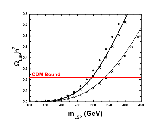
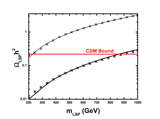
Figure 3: $\Omega_{\rm LSP}h^{2}$ versus $m_{\rm LSP}$ for $m^{\rm c}_{b}(M_{Z})=2.68~{}{\rm GeV},\mu>[<]~{}0$ and $\Delta_{\tilde{\tau}_{2}}=1.5~{}[0]$ (left [right] plot). The thick (faint) solid line is obtained by micrOMEGAs with (without) loop QCD corrections [coannihilations] while the thick (faint) crosses by our code. The stars are obtained by our code, including SUSY corrections, too. The upper bound on $\Omega_{\rm LSP}h^{2}~{}(=0.22)$ is also depicted.

A further comparison is displayed in Fig. 3 (left plot), where we depict $\Omega_{\rm LSP}h^{2}$ versus $m_{\rm LSP}$ for $\mu>0,\Delta_{\tilde{\tau}_{2}}=1.5$ and $m_{b}(M_{Z})=2.68~{}{\rm GeV}$. $\Omega_{\rm LSP}h^{2}$ is calculated by micrOMEGAs [our code] with (thick solid line [crosses]) or without (faint solid line [crosses]) the inclusion of the loop QCD corrections to $g_{Aff}$ couplings. The stars are obtained by our code, including the SUSY corrections, too.

3.3 INCLUDING BINO-STAU COANNIHILATIONS

Table 3: INCLUDED FEYNMAN DIAGRAMS

INITIAL STATE	FINAL STATE	INTERACTION CHANNELS
$\tilde{\chi}\tilde{\chi}$	$f\bar{f}$	$s(h),s(H),s(A),s(Z)$
	( $f$: Fermions)	$t(\mbox{$\tilde{f}$}_{1,2}),u(\mbox{$\tilde{f}$}_{1,2})$
	$H^{\pm}W^{\mp}$	$s(h),s(H),s(A),t(\mbox{${\tilde{\chi}_{i}^{\pm}}$}),u(\mbox{${\tilde{\chi}_{i}^{\pm}}$})$
	$hA,ZH$	$s(A),s(Z),t(\mbox{${\tilde{\chi}_{i}^{0}}$}),u(\mbox{${\tilde{\chi}_{i}^{0}}$})$
$\tilde{\chi}\tilde{\tau}_{2}$	$\tau h,\tau H,\tau Z$	$s(\tau),t(\tilde{\tau}_{1,2}),u(\tilde{\chi}^{0}_{i})$
	$\tau A$	$s(\tau),t(\tilde{\tau}_{1}),u(\tilde{\chi}^{0}_{i})$
	$\tau\gamma$	$s(\tau),t(\tilde{\tau}_{2})$
	$\mbox{$\nu_{\tau}$}H^{-},\mbox{$\nu_{\tau}$}W^{-}$	$s(\tau),t(\tilde{\chi}^{\pm}_{i}),u(\tilde{\nu}_{\tau})$
$\tilde{\tau}_{2}\tilde{\tau}_{2}$	$\tau\tau$	$t(\tilde{\chi}^{0}_{i}),u(\tilde{\chi}^{0}_{i})$
$\tilde{\tau}_{2}\tilde{\tau}_{2}^{\ast}$	$hh,hH,HH,ZZ$	$s(h),s(H),t(\tilde{\tau}_{1,2}),u(\tilde{\tau}_{1,2}),{\rm PI}$
	$AA$	$s(h),s(H),t(\tilde{\tau}_{1}),u(\tilde{\tau}_{1}),{\rm PI}$
	$H^{+}H^{-},W^{+}W^{-}$	$s(h),s(H),s(\gamma),s(Z),t(\tilde{\nu}_{\tau}),{\rm PI}$
	$H^{\pm}W^{\mp}$	$s(h),s(H),t(\tilde{\nu}_{\tau})$
	$AZ$	$s(h),s(H),t(\tilde{\tau}_{1}),u(\tilde{\tau}_{1})$
	$\gamma\gamma,\gamma Z$	$t(\tilde{\tau}_{2}),u(\tilde{\tau}_{2}),{\rm PI}$
	$t\bar{t},b\bar{b}$	$s(h),s(H),s(\gamma),s(Z)$
	$\tau\bar{\tau}$	$s(h),s(H),s(\gamma),s(Z),t(\tilde{\chi})$

Bino-stau coannihilations come into play, when $\Delta_{\tilde{\tau}_{2}}\lesssim 0.25$. $\Omega_{\rm LSP}h^{2}$ is not any more inverse proportional to $\langle v\sigma_{\tilde{\chi}\tilde{\chi}}\rangle$ but to an effective $\langle v\sigma\rangle$ which includes, in addition, $\langle v\sigma_{\tilde{\tau}_{2}\tilde{\chi}[\tilde{\tau}_{2}]}\rangle$ with a weight factor $\exp{\left(-[2]\Delta_{\tilde{\tau}_{2}}x^{-1}_{\rm F}\right)}$, where $x^{-1}_{\rm F}=m_{\rm LSP}/T_{\rm F}$ $\sim 25$ and $T_{\rm F}$ the freeze out temperature [27]. Consequently, for given $m_{\rm LSP}$, $\Delta_{\tilde{\tau}_{2}}$ regulates the degeneracy amount. The strongest possible reduction is achieved for $\Delta_{\tilde{\tau}_{2}}=0$.

The computation of $\Omega_{\rm LSP}h^{2}$ in this regime, can be realized by using exclusively the low velocity expansion of $\langle v\sigma\rangle$. The thermal average has been performed, following the Ref. [21]. The included set of (co)annihilation processes (in accord with the tables in Refs. [28]) is shown in the Table 3 (we apply the notation of Ref. [14] and PI stands for “point interaction”). The relevant matrix elements are evaluated with the help of the FeynCalc package [30]. Our results are compared with micrOMEGAs, in the Table 4 for 3 test points. Besides the values of $\Omega_{\rm LSP}h^{2}$ and $x_{\rm F}^{-1}$, we display, also, the contribution of all the channels, beyond $0.3\%$. As we can observe, our differences are small in most cases.

The importance of CAM, in deriving an upper bound on $m_{\rm LSP}$ from Eq. (24), can be easily concluded from Fig. 3 (right plot), where we depict $\Omega_{\rm LSP}h^{2}$ versus $m_{\rm LSP}$ for $\mu<0,\Delta_{\tilde{\tau}_{2}}=0$ and $m^{\rm c}_{b}(M_{Z})=2.68~{}{\rm GeV}$. $\Omega_{\rm LSP}h^{2}$ is calculated with (thick solid line [crosses]) or without (faint solid line [crosses]) the inclusion of bino-stau coannihilations using micrOMEGAs [our code]. We see that the reduction of $\Omega_{\rm LSP}h^{2}$ caused by the CAM is dramatic (a factor of 10). This increases the upper bound on $m_{\rm LSP}$ derived from Eq. (24) from about $200~{}{\rm GeV}$ to $900~{}{\rm GeV}$.

Table 4: COMPARISON OF $\Omega_{\rm LSP}h^{2}$ CALCULATIONS

MODEL PARAMETERS
($\mu<0,~{}m^{\rm c}_{b}(M_{Z})=2.68~{}{\rm GeV},~{}A_{0}=0~{}{\rm GeV}$)
$\tan\beta$	51.2		50.0		49.4
$M_{1/2}~{}({\rm GeV})$	1877		859		596
$m_{0}~{}({\rm GeV})$	957		463		357
$m_{A}~{}({\rm GeV})$	$466$		214		130
$m_{\rm LSP}~{}({\rm GeV})$	865		386		264
$\Delta_{\tilde{\tau}_{2}}$	0.00		0.05		0.10
$\Omega_{\rm LSP}h^{2}$ CALCULATIONS
CODE :	micr-	GLP	micr-	GLP	micr-	GLP
	OMEGAs		OMEGAs		OMEGAs
PROCESSES WHICH CONTRIBUTE MORE THAN $0.3\%$
PROCESS	CONTRIBUTION ($\%$)
$\tilde{\chi}\tilde{\chi}\rightarrow f\bar{f}$	0.4	0.5	8.4	10.6	25.7	30.5
$\tilde{\chi}\tilde{\chi}\rightarrow H^{\pm}W^{\mp}$	0.8	0.7	9.4	10.1	18.6	19.6
$\tilde{\chi}\tilde{\chi}\rightarrow HZ$	0.4	0.2	5.1	3.8	11.2	10.4
$\tilde{\chi}\tilde{\chi}\rightarrow hA$	0.4	0.3	5.2	4.3	11.0	9.3
$\tilde{\chi}\tilde{\chi}\rightarrow hH$	-	-	-	-	0.3	0.3
$\tilde{\chi}\tilde{\chi}\rightarrow AZ$	-	-	-	-	0.3	0.2
$\tilde{\chi}\tilde{\tau}_{2}\rightarrow\tau h$	1.4	0.4	8.0	6.9	7.1	6.1
$\tilde{\chi}\tilde{\tau}_{2}\rightarrow\tau H$	3.0	2.8	4.8	4.6	2.6	2.4
$\tilde{\chi}\tilde{\tau}_{2}\rightarrow\tau A$	3.0	3.3	4.7	5.3	2.7	2.8
$\tilde{\chi}\tilde{\tau}_{2}\rightarrow\nu_{\tau}H^{-}$	5.8	6.0	8.5	9.1	4.4	4.4
$\tilde{\chi}\tilde{\tau}_{2}\rightarrow\nu_{\tau}W^{-}$	0.6	0.5	1.5	1.3	0.9	0.7
$\tilde{\chi}\tilde{\tau}_{2}\rightarrow\tau\gamma$	7.9	7.7	11.9	12.3	6.4	6.3
$\tilde{\chi}\tilde{\tau}_{2}\rightarrow\tau Z$	2.7	2.7	4.8	5.0	2.8	2.7
$\tilde{\tau}_{2}\tilde{\tau}_{2}\rightarrow\tau\tau$	19.0	19.2	5.5	5.7	0.9	0.8
$\tilde{\tau}_{2}\tilde{\tau}_{2}^{\ast}\rightarrow hh$	8.0	8.2	4.2	3.9	0.8	0.6
$\tilde{\tau}_{2}\tilde{\tau}_{2}^{\ast}\rightarrow HH$	3.0	3.2	0.9	0.9	-	-
$\tilde{\tau}_{2}\tilde{\tau}_{2}^{\ast}\rightarrow AA$	3.0	3.2	0.9	0.9	-	-
$\tilde{\tau}_{2}\tilde{\tau}_{2}^{\ast}\rightarrow H^{+}H^{-}$	5.6	6.2	1.3	1.5	-	-
$\tilde{\tau}_{2}\tilde{\tau}_{2}^{\ast}\rightarrow H^{\pm}W^{\mp}$	0.4	0.4	-	-	-	-
$\tilde{\tau}_{2}\tilde{\tau}_{2}^{\ast}\rightarrow W^{+}W^{-}$	13.8	14.4	4.4	4.6	0.6	0.6
$\tilde{\tau}_{2}\tilde{\tau}_{2}^{\ast}\rightarrow ZZ$	7.3	7.7	2.3	2.4	0.3	0.3
$\tilde{\tau}_{2}\tilde{\tau}_{2}^{\ast}\rightarrow\gamma\gamma$	5.7	5.3	1.7	1.7	0.3	0.2
$\tilde{\tau}_{2}\tilde{\tau}_{2}^{\ast}\rightarrow\gamma Z$	3.0	3.2	0.7	0.8	-	-
$\tilde{\tau}_{2}\tilde{\tau}_{2}^{\ast}\rightarrow t\bar{t}$	4.1	3.0	4.5	3.5	0.9	0.6
$x^{-1}_{\rm F}$	25.97	26.03	25.51	25.48	24.82	24.84
$\Omega_{\rm LSP}h^{2}$	0.221	0.205	0.221	0.221	0.220	0.216

4 PHENOMENOLOGICAL CONSTRAINTS

A lower bound on $m_{\rm LSP}$ can be derived by imposing a number of phenomenological constraints [10, 13, 20, 23]. These result from:

i. The Higgs boson masses. The relevant for our analysis is the $95\%$ c.l. LEP bound [31] on the lightest CP-even neutral Higgs boson, $h$ mass

$$m_{h}\gtrsim 114.4~{}{\rm GeV}$$ (26)

which gives a [almost always the absolute] lower bound on $m_{\rm LSP}$ for $\mu<[>]~{}0$. The SUSY contributions to $m_{h}$ are calculated at two-loop by using the FeynHiggsFast [32] program included in micrOMEGAs package [25].

ii. The deviation $\delta a_{\mu}$ of the muon anomalous magnetic moment measured value, $a_{\mu}$, from its predicted in the SM, $a^{\rm SM}_{\mu}$. The latter is not yet stabilized mainly due to the instability of the hadronic vacuum polarization contribution. According to the most updated [35] evaluation of this contribution, the findings based on $e^{+}e^{-}$ data and on $\tau$-decay data are inconsistent with each other. Combining these results with the recent experimental measurements on $a_{\mu}$ [33], we obtain the following $95\%$ c.l. ranges:

$$\mbox{\sf a)}\hskip 16.9pt11.3\times 10^{-10}\lesssim\delta a_{\mu} \mbox{\sf b)}~{}~{}\delta a_{\mu}\lesssim 56.1\times 10^{-10}~{}~{}~{}~{}\mbox{$e^{+}e^{-}$-based}$$ and (27)

$$\vspace*{19pt}\mbox{\sf a)}~{}-11.6\times 10^{-10}\lesssim\delta a_{\mu} \mbox{\sf b)}~{}~{}\delta a_{\mu}\lesssim 30.4\times 10^{-10}~{}~{}~{}~{}\mbox{$\tau$-based}$$ and (28)

The SUSY contribution to the $\delta a_{\mu}$ is calculated by using the formulae of Ref. [34] in accord with micrOMEGAs [25] and the result is posi[nega]-tive for $\mu>[<]~{}0$. A lower bound on $m_{\rm LSP}$ can be derived for $\mu>[<]~{}0$ from Eq. (27b) [(28a)] and an optimistic upper bound for $\mu>0$ from Eq. (27a) which, however is not imposed as an absolute constraint.

iii. The inclusive branching ratio of $b\rightarrow s\gamma$, ${\rm BR}(b\rightarrow s\gamma)$. Taking into account the recent experimental results [36] on this ratio and combining appropriately the experimental and theoretical involved errors [1], we obtain the following $95\%$ c.l. range:

$$\mbox{\sf a)}~{}~{}1.9\times 10^{-4}\lesssim{\rm BR}(b\rightarrow s\gamma)~{}~{}~{}~{}\mbox{and}~{}~{}~{}~{}\mbox{\sf b)}~{}~{}{\rm BR}(b\rightarrow s\gamma)\lesssim 4.6\times 10^{-4}$$ (29)

To calculate ${\rm BR}(b\rightarrow s\gamma)$ we used an updated version of the code contained in the current version of micrOMEGAs [37]. This code represents a complete update respect the one used in the first paper of Ref.  [1]. The SM contribution is calculated using the Refs. [38]. The charged Higgs boson [SUSY] contribution is evaluated by including the next-to-leading order QCD [SUSY resummed] corrections and $\tan\beta$ enhanced contributions from Refs. [39]. A lower bound on $m_{\rm LSP}$ can be derived for $\mu>[<]~{}0$ from Eq. (29a) [(29b)] with the latter being much more restrictive.

5 CONCLUSIONS-OPEN ISSUES

Allowing $m^{\rm c}_{b}(M_{Z})$ to vary in its 95$\%$ c.l. range, Eq. (5) and using the previous Cosmo-Phenomenological restrictions, we can delineate the parameter space of the model on the $m_{\rm LSP}-\Delta_{\tilde{\tau}_{2}}$ plane in Figs. 4 and 5. For simplicity, we do not show bounds from less restrictive constraints, Eq. (27b) and (29a) [(26)] for $\mu>[<]~{}0$.

For $\mu>0$, the allowed space of parameters (depicted in Fig. 5) is wide as regards both $\Delta_{\tilde{\tau}_{2}}$ (because of the $A$PE) and $m_{\rm LSP}$ (because of the CAM) range. Especially,

$$\Big{(}\mbox{From Eq. (\ref{mhb})}:\Big{)}\>\>\>159~{}{\rm GeV}\lesssim m_{\rm LSP}\lesssim 720~{}[371]\>{\rm GeV}\>\>\>\Big{(}:\mbox{From Eq. (\ref{cdmb}) [(\ref{g2e}{\sf a})]}\Big{)}$$

(taking the less restrictive values of the various constraints). The changes on the upper limit of the allowed area from a possible inclusion of the SUSY corrections (sec. 3.2) in the $\Omega_{\rm LSP}h^{2}$ calculation are almost invisible. On the contrary, let $\alpha_{s}(M_{Z})$ vary in its $95\%$ c.l. experimental range $0.1145-0.1225$ with the corresponding range of $m^{\rm c}_{b}(M_{Z})$ to be ($2.62-3.16)~{}{\rm GeV}$, the allowed area can further enlarge until the dotted line in the Fig. 4.

On the other hand, for $\mu<0$, the competition of the various Cosmo-Phenomenological constraints is more dangerous and, finally, disastrous for this case, since:

$$\Big{(}\mbox{From Eq. (\ref{g2t}{\sf a})}:\Big{)}\>\>\>387~{}{\rm GeV}\lesssim m_{\rm LSP}\lesssim 873\>\>\>{\rm GeV}\>\>\> \Big{(}:\mbox{From Eq. (\ref{cdmb})}\Big{)}$$

and $$m_{\rm LSP}\gtrsim 1305\>{\rm GeV}\>\>\> \Big{(}:\mbox{From Eq. (\ref{bsgb}{\sf b})}\Big{)}$$

Despite the strong presence of the CAM ($\Delta_{\tilde{\tau}_{2}}\lesssim 0.05$) we are, evidently, left without simultaneously allowed region, as it is shown in Fig. 5.

Figure 4: The allowed area on the $m_{\rm LSP}$-$\Delta_{\tilde{\tau}_{2}}$ plane for $\mu>0$ and $2.68~{}{\rm GeV}\lesssim m^{\rm c}_{b}(M_{Z})\lesssim 3.09~{}{\rm GeV}$. Shown is, also, the [optimistic] upper bound from Eq. [(27a)] (24) with $2.61~{}{\rm GeV}\lesssim m_{b}(M_{Z})\lesssim 3.15~{}{\rm GeV}$, [dashed] dotted line.

Figure 5: Disconnected areas on the $m_{\rm LSP}$-$\Delta_{\tilde{\tau}_{2}}$ plane for $\mu<0$ and $2.68~{}{\rm GeV}\lesssim m^{\rm c}_{b}(M_{Z})\lesssim 3.09~{}{\rm GeV}$ allowed by various restrictions indicated in the plot.

Constructions similar to this presented in sec. 2.2 may be useful for other SUSY GUTs, too. The $SO(10)$ or $SU(5)$ SUSY GUTs in their simple realization lead to complete [12, 13] or $b-\tau$ [10, 40] YU, with the latter being viable only for $\mu<0$ and consequently, quite disfavored from the bounds of Eq. (27). Also, the large values of $\tan\beta$ predicted in these models, can enhance the neutralino detection rates with universal [41] or non universal [10] asymptotic gaugino masses. Furthermore, the extra higgs fields used in sec. 2.2 have interesting consequences to the inflation mechanism, as it is pointed out in Ref. [42].

References

• [1] M.E. Gómez, G. Lazarides and C. Pallis, Nucl. Phys. B638, 165 (2002) [\hepph0203131]; \hepph0301064.
• [2] R. Jeannerot, S. Khalil, G. Lazarides and Q. Shafi, JHEP 10, 012 (2000) [\hepph0002151].
• [3] I. Antoniadis and G.K. Leontaris, Phys. Lett. B 216, 333 (1989).
• [4] G.L. Kane, C. Kolda, L. Roszkowski and J.D. Wells, Phys. Rev. D 49, 6173 (1994) [\hepph9312272].
• [5] L. Hall, R. Rattazzi and U. Sarid, Phys. Rev. D 50, 7048 (1994) [\hepph9306309]; M. Carena, M. Olechowski, S. Pokorski and C.E.M. Wagner, Nucl. Phys. B426, 269 (1994) [\hepph9402253].
• [6] D. Pierce, J. Bagger, K. Matchev and R. Zhang, Nucl. Phys. B491, 3 (1997) [\hepph9606211].
• [7] M. Carena, D. Garcia, U. Nierste and C.E.M. Wagner, Nucl. Phys. B577, 88 (2000) [\hepph9912516].
• [8] SUGRA Working Group Collaboration (S. Abel et al.), \hepph0003154.
• [9] H. Baer, J. Ferrandis, K. Melnikov and X. Tata, Phys. Rev. D 66, 0740007 (2002) [\hepph0207126].
• [10] U. Chattopadhyay, A. Corsetti and P. Nath, Phys. Rev. D 66, 035003 (2002) [\hepph0201001].
• [11] S.F. King and M. Oliveira, Phys. Rev. D 63, 015010 (2001) [\hepph0008183].
• [12] T. Blažek, R. Dermíšek and S. Raby, Phys. Rev. Lett. 88 111804, (2002) [\hepph0107097]; Phys. Rev. D 65, 115004 (2002) [\hepph0201081].
• [13] H. Baer and J. Ferrandis, Phys. Rev. Lett. 87, 211803 (2001) [\hepph0106352]; H. Baer et al., Phys. Rev. D 63, 015007 (2001) [\hepph0005027]; D. Auto et al., \hepph0302155; K. Tobe and J.D. Wells, \hepph0301015.
• [14] M.E. Gómez, G. Lazarides and C. Pallis, Phys. Rev. D 61, 123512 (2000) [\hepph9907261]; Phys. Lett. B 487, 313 (2000) [\hepph0004028].
• [15] M.E. Gómez and C. Pallis, \hepph0303094 (to appear in the SUSY02 Proceedings).
• [16] H. Goldberg, Phys. Rev. Lett. 50, 1419 (1983); J.R. Ellis, J.S. Hagelin, D.V. Nanopoulos, K.A. Olive and M. Srednicki, Nucl. Phys. B238, 453 (1984).
• [17] C. Pryke, et al. ApJ568200246 [\astroph0104490].
• [18] A.B. Lahanas, D.V. Nanopoulos and V.C. Spanos, Phys. Rev. D 62, 023515 (2000) [\hepph9909497].
• [19] J. Ellis, T. Falk and K.A. Olive, Phys. Lett. B 444, 367 (1998) [\hepph9810360].
• [20] J. Ellis, T. Falk, G. Ganis, K.A. Olive and M. Srednicki, Phys. Lett. B 510, 236 (2001) [\hepph0102098].
• [21] J. Ellis, T. Falk, K.A. Olive and M. Srednicki, Astropart. Phys. 13, 181 (2000) (E) ibid. 15, 413 (2001) [\hepph9905481].
• [22] J. Ellis, K. Olive and Y. Santoso, Astropart. Phys. 18, 395 (2003) [\hepph0112113].
• [23] H. Baer, C. Balázs and A. Belyaev, JHEP 03, 042 (2002) [\hepph0202076].
• [24] J. Edsjö, M. Schelke, P. Ullio and P. Gondolo, \hepph0301106.
• [25] G. Bélanger, F. Boudjema, A. Pukhov and A. Semenov, Comput. Phys. Commun. 149, 103 (2002), [\hepph0112278]; \hepph0210327.
• [26] P. Gondolo, J. Edsjö, L. Bergström, P. Ullio and E.A. Baltz, \astroph0012234.
• [27] P. Gondolo and G. Gelmini, Nucl. Phys. B360, 145 (1991).
• [28] T. Nihei, L. Roszkowski and R. Ruiz de Austri, JHEP 03, 031 (2002) [\hepph0202009]; ibid. 07, 024 (2002) [\hepph0206266].
• [29] M. Spira, Fortsch. Phys. 46 203, 1998 [\hepph9705337] and references therein.
• [30] R. Mertig, The FeynCalc Book, http://www.feyncalc.org
• [31] ALEPH, DELPHI, L3 and OPAL Collaborations, The LEP Higgs working group for Higgs boson searches, \hepex0107029, LHWG-NOTE/2002-01
http://lephiggs.web.cern.ch/LEPHIGGS/papers/July2002_SM/index.html
• [32] S. Heinemeyer, W. Hollik and G. Weiglein, \hepph0002213.
• [33] G.W. Bennett et al. (Muon $g$-2 Collaboration), Phys. Rev. Lett. 89, 101804 (2002); 89, 129903(E) (2002) [\hepex0208001].
• [34] S.P. Martin and J.D. Wells, Phys. Rev. D 64, 035003 (2001) [\hepph0103067].
• [35] M. Davier, S. Eidelman, A. Höcker and Z. Zhang, \hepph0208177.
• [36] R. Barate et al. (ALEPH Collaboration), Phys. Lett. B 429, 169 (1998); K. Abe et al. (BELLE Collaboration), Phys. Lett. B 511, 151 (2001) [\hepex0103042]; S. Chen et al. (CLEO Collaboration), Phys. Rev. Lett. 87, 251807 (2001) [\hepex0108032].
• [37] G. Bélanger, F. Boudjema, A. Pukhov and A. Semenov, private communication.
• [38] A.L. Kagan and M. Neubert, Eur. Phys. J. C 7, 5 (1999) [\hepph9805303]; P. Gambino and M. Misiak, Nucl. Phys. B611, 338 (2001) [\hepph0104034].
• [39] M. Ciuchini, G. Degrassi, P. Gambino and G. Giudice, Nucl. Phys. B527, 21 (1998) [\hepph9710335]; G. Degrassi, P. Gambino and G.F. Giudice, JHEP 12, 009 (2000) [\hepph0009337].
• [40] W. de Boer, M. Huber, A.V. Gladyshev and D.I. Kazakov, Eur. Phys. J. C 20, 689 (2001) [\hepph0102163].
• [41] M.E Gómez and J.D. Vergados, Phys. Lett. B 512, 252 (2001) [\hepph0012020]; \hepph0105114; \hepph0105115.
• [42] R. Jeannerot, S. Khalil and G. Lazarides, JHEP 07, 069 (2002) [\hepph0207244].