Abstract

I review the physics of the Higgs sector in the Standard Model and its minimal supersymmetric extension, the MSSM. I will discuss the prospects for discovering the Higgs particles at the upgraded Tevatron, at the Large Hadron Collider, and at a future high–energy $e^{+}e^{-}$ linear collider with centre–of–mass energy in the 350–800 GeV range, as well as the possibilities for studying their fundamental properties. Some emphasis will be put on the theoretical developments which occurred in the last two years.

1. A brief introduction

The search for Higgs bosons is the primary mission of present and future high–energy colliders. Detailed theoretical and experimental studies performed in the last few years, have shown that the single neutral Higgs boson that is predicted in the Standard Model (SM) [1] could be discovered at the upgraded Tevatron, if it is relatively light and if enough integrated luminosity is collected [2, 3] and can be detected at the LHC [3, 4] over its entire mass range 114.4 GeV $\raisebox{-3.69899pt}{~{}\shortstack{$<$ \\ [-0.07cm] $\sim$}}~{}M_{H}\raisebox{-3.69899pt}{~{}\shortstack{$<$ \\ [-0.07cm] $\sim$}}~{}1$ TeV in many redundant channels; see Fig. 1. In the context of the Minimal Supersymmetric Standard Model (MSSM), where the Higgs sector is extended to contain two CP–even neutral Higgs bosons $h$ and $H$, a pseudoscalar $A$ boson and a pair of charged scalar particles $H^{\pm}$ [1], it has been shown that the lighter $h$ boson cannot escape detection at the LHC and that in large areas of the parameter space, more than one Higgs particle can be found; see Fig. 1.

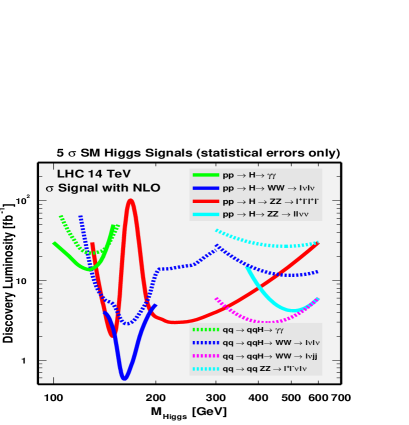
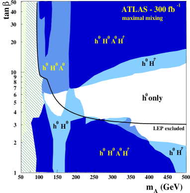
Figure 1: The integrated luminosity needed for the discovery of the SM Higgs boson at the LHC in various production and decay channels (left) and the number of Higgs particles that can be detected in the MSSM $(\tan\beta,M_{A})$ parameter space (right); from Ref. [5].

Should we then declare that we have done our homework and wait peacefully for the LHC to start operation? Well, discovering the Higgs boson is not the entire story, and another goal, just as important, would be to probe the electroweak symmetry breaking mechanism in all its facets. Once the Higgs boson is found, the next step would therefore be to perform very high precision measurements to explore all its fundamental properties. To achieve this goal in great detail, one needs to measure all possible cross sections and decay branching ratios of the Higgs bosons to derive their masses, their total decay widths, their couplings to the other particles and their self–couplings, their spin–parity quantum numbers, etc. This needs very precise theoretical predictions and more involved theoretical and experimental studies. In particular, all possible production and decay channels of the Higgs particles, not only the dominant and widely studied ones allowing for clear discovery, should be investigated. This also requires complementary detailed studies at future $e^{+}e^{-}$ linear colliders, where the clean environment and the expected high luminosity allow for very high precision measurements [6, 7].

In this talk, I will summarize the studies that were performed recently in the SM and MSSM Higgs sectors. In the next section, after summarizing the present constraints, I will discuss the new developments in the calculation of the Higgs boson spectrum and decay branching ratios. In in sections 3 and 4, we will discuss the developments in Higgs production at the LHC and Tevatron hadron colliders and at a future $e^{+}e^{-}$ machine with a c.m. energy below 1 TeV. A brief conclusion will be presented in section 5.

2. Higgs spectrum and decay branching ratios

In the SM, the profile of the Higgs boson is uniquely determined once $M_{H}$ is fixed [1]: the decay width and branching ratios, as well as the production cross sections, are given by the strength of the Yukawa couplings to fermions and gauge bosons, which is set by the masses of these particles. There are two experimental constraints on this free parameter.

The SM Higgs boson has been searched for at LEP in the Higgs–strahlung process $e^{+}e^{-}\to HZ$ for c.m.  energies up to $\sqrt{s}=209$ GeV and with a large collected luminosity. In summer 2002, the final results of the four LEP collaborations were published [and some changes with respect to the original publications occurred, in particular inclusion of more statistics, revision of backgrounds, and reassessment of systematic errors]. When these results are combined, an upper limit $M_{H}\geq 114.4$ GeV is established at the 95% confidence level [9]. However, this upper limit, in the absence of additional events with respect to SM predictions, was expected to be $M_{H}>115.3$ GeV; the reason is that there is a $1.7\sigma$ excess [compared to the value $2.9\sigma$ reported at the end of 2000] of events for a Higgs boson mass in the vicinity of $M_{H}=116$ GeV [9].

The second constraint comes from the accuracy of the electroweak observables measured at LEP, the SLC and the Tevatron, which provides sensitivity to $M_{H}$: the Higgs boson contributes logarithmically, $\propto\log(M_{H}/M_{W})$, to the radiative corrections to the $W/Z$ boson propagators and alters these observables. The status, as in summer 2002, is summarized in Fig. 2, which shows the $\Delta\chi^{2}$ of the fit to electroweak precision measurements as a function of $M_{H}$ [10]. When all available data [i.e. the Z–boson pole LEP and SLC data, the measurement of the $W$ boson mass and total width, the top–quark mass and the controversial NuTeV result] are taken into account, one obtains a Higgs boson mass of $M_{H}=81^{+42}_{-33}$ GeV, leading to a 95% confidence level upper limit of $M_{H}<193$ GeV. These values are relatively stable when the NuTeV result is excluded from the fit, or when a different value for the hadronic contribution to the QED coupling $\alpha$ is used.

However, theoretical constraints can also be derived from assumptions on the energy range within which the SM is valid before perturbation theory breaks down and New Physics should appear. If $M_{H}\raisebox{-3.69899pt}{~{}\shortstack{$>$ \\ [-0.07cm] $\sim$}}~{}1$ TeV, the longitudinal $W$ and $Z$ bosons would interact strongly; to ensure unitarity in their scattering at high energies, one needs $M_{H}\raisebox{-3.69899pt}{~{}\shortstack{$<$ \\ [-0.07cm] $\sim$}}~{}710$ GeV at tree–level [11]. In addition, the quartic Higgs self–coupling, which at the weak scale is fixed by $M_{H}$, grows logarithmically with energy and a cut–off $\Lambda$ should be imposed before it grows beyond any bound. The condition $M_{H}\raisebox{-3.69899pt}{~{}\shortstack{$<$ \\ [-0.07cm] $\sim$}}~{}\Lambda$ sets an upper limit at $M_{H}\sim 630$ GeV. Furthermore, top quark loops tend to drive the coupling to negative values, for which the vacuum becomes unstable. Requiring the SM to be extended to the GUT scale, $\Lambda\sim 10^{16}$ GeV, the Higgs mass should lie in the range 130 GeV $\raisebox{-3.69899pt}{~{}\shortstack{$<$ \\ [-0.07cm] $\sim$}}~{}M_{H}\raisebox{-3.69899pt}{~{}\shortstack{$<$ \\ [-0.07cm] $\sim$}}~{}180$ GeV [12].

Figure 2: The $\Delta\chi^{2}$ of the fit to electroweak precision data as a function of $M_{H}$. The solid line is when all data are included and the blue band is the estimated theoretical error from unknown higher order corrections. The effect of excluding the NuTeV measurement and the use of a different value for $\Delta\alpha_{\rm had}$ are also shown. The vertical band shows the 95% CL exclusion limit on $M_{H}$ from direct searches. From Ref. [10].

In the MSSM, two doublets of Higgs fields are needed to break the electroweak symmetry, leading to two CP–even neutral $h,H$ bosons, a pseudoscalar $A$ boson and a pair of charged scalar particles, $H^{\pm}$ [1]. Besides the four masses, two additional parameters define the properties of the particles: a mixing angle $\alpha$ in the neutral CP–even sector, and the ratio of the two vacuum expectation values, $\tan\beta$. Because of supersymmetry constraints, only two of them, e.g.  $M_{A}$ and $\tan\beta$, are in fact independent at tree–level. While the lightest Higgs mass is bounded by $M_{h}\leq M_{Z}$, the masses of the $A,H$ and $H^{\pm}$ states are expected to be below ${\cal O}(1$ TeV). However, mainly because of the heaviness of the top quark, radiative corrections are very important: the leading part grows as the fourth power of $m_{t}$ and logarithmically with the common top squark mass $M_{S}$; the stop trilinear coupling $A_{t}$ also plays an important role and maximizes the correction for the value $A_{t}\sim 2M_{S}$. For a recent review, see Ref. [13].

Recently, new calculations of the two–loop radiative corrections have been performed [14]. Besides the already known ${\cal O}(\alpha_{t}\alpha_{s})$ correction, the contributions at ${\cal O}(\alpha_{t}^{2})$ and ${\cal O}(\alpha_{s}\alpha_{b})$ have been derived. By an appropriate use of the effective potential approach, one obtains simple analytic formulae for arbitrary values of $M_{A}$ and of the parameters in the stop sector. In a large region of the parameter space, the ${\cal O}(\alpha_{t}^{2})$ corrections are sizeable, increasing the predicted value for $M_{h}$ [for given $\tan\beta$ and $M_{A}$ inputs] by several GeV. This is exemplified in Fig. 3, where the value of $M_{h}$ is shown as a function of $M_{A}$ for $\tan\beta=2$ and 20 in various approximations. As can be seen, the upper bound on $M_{h}$ can reach the level of 130 GeV if the corrections due to $\alpha_{t}$ are included. At large values of $\tan\beta$ where the Yukawa coupling of the $b$–quark becomes rather large, a further increase of a few GeV is obtained if the ${\cal O}(\alpha_{s}\alpha_{b})$ correction is included.

Figure 3: The value of the lightest $h$ boson mass as a function of $M_{A}$ in the MSSM for $\tan\beta=2$ and 20 in the maximal mixing scenario $X_{t}\sim A_{t}\sim 2M_{S}\sim 2$ TeV. The long–dashed line shows the result at one–loop, while the full line shows the two–loop result including the full ${\cal O}(\alpha_{t}\alpha_{s})$ and ${\cal O}(\alpha_{t}^{2})$ corrections; from Ref. [14].

Note that these important radiative corrections are now being implemented in the three new codes for the determination of the MSSM particle spectrum, which appeared in the last year: Softsusy, SuSpect and Spheno [15].

The production and the decays of the MSSM Higgs bosons depend strongly on their couplings to gauge bosons and fermions. The pseudoscalar has no tree level couplings to gauge bosons, and its couplings to down–(up)–type fermions are (inversely) proportional to $\tan\beta$. It is also the case for the couplings of the charged Higgs particle to fermions, which are a mixture of scalar and pseudoscalar currents and depend only on $\tan\beta$. For the CP–even Higgs bosons, the couplings to down–(up)–type fermions are enhanced (suppressed) with respect to the SM Higgs couplings for $\tan\beta>1$. They share the SM Higgs couplings to vector bosons since they are suppressed by $\sin(\beta-\alpha)$ and $\cos(\beta-\alpha)$ factors, respectively for $h$ and $H$. If the pseudoscalar mass is large, the $h$ boson mass reaches its upper limit [which depends on the value of $\tan\beta$] and the angle $\alpha$ reaches the value $\alpha=\beta-\frac{1}{2}\pi$. The $h$ couplings to fermions and gauge bosons are then SM–like, while the heavier CP–even $H$ and charged $H^{\pm}$ bosons become degenerate in mass with $A$. In this decoupling limit, it is very difficult to distinguish the SM and MSSM Higgs sectors.

The constraints on the MSSM Higgs particles masses mainly come from the negative searches at LEP2 [9] in the Higgs–strahlung process, $e^{+}e^{-}\to Z+h/H$, and pair production process, $e^{+}e^{-}\to A+h/H$, with the Higgs bosons mainly decaying into $b\bar{b}$ pairs [these processes will be discussed later]. In the decoupling limit where the $h$ boson has SM–like couplings to $Z$ bosons, the limit $M_{h}\raisebox{-3.69899pt}{~{}\shortstack{$>$ \\ [-0.07cm] $\sim$}}~{}114.4$ GeV from the $e^{+}e^{-}\to hZ$ process holds. This constraint rules out $\tan\beta$ values larger than $\tan\beta\raisebox{-3.69899pt}{~{}\shortstack{$>$ \\ [-0.07cm] $\sim$}}~{}2.5$. From the $e^{+}e^{-}\to Ah$ process, one obtains the absolute limits $M_{h}\raisebox{-3.69899pt}{~{}\shortstack{$>$ \\ [-0.07cm] $\sim$}}~{}91$ GeV and $M_{A}\raisebox{-3.69899pt}{~{}\shortstack{$>$ \\ [-0.07cm] $\sim$}}~{}91.9$ GeV, for a maximal $ZhA$ coupling. More details are given in the talk by P. Igo-Kemenes.

Let us now discuss the Higgs decay modes and branching ratios (BR) [16] and start with the SM case [Fig. 4]. In the “low–mass” range, $M_{H}\raisebox{-3.69899pt}{~{}\shortstack{$<$ \\ [-0.07cm] $\sim$}}~{}130$ GeV, the Higgs boson decays into a large variety of channels. The main mode is by far the decay into $b\bar{b}$ with BR $\sim$ 90% followed by the decays into $c\bar{c}$ and $\tau^{+}\tau^{-}$ with BRs $\sim$ 5%. Also of significance is the top–loop mediated decay into gluons, which occurs at the level of $\sim$ 5%. The top and $W$–loop mediated $\gamma\gamma$ and $Z\gamma$ decay modes are very rare with BRs of ${\cal O}(10^{-3})$ [however, they lead to clear signals and are interesting, since they are sensitive to new heavy particles]. In the “high–mass” range, $M_{H}\raisebox{-3.69899pt}{~{}\shortstack{$>$ \\ [-0.07cm] $\sim$}}~{}130$ GeV, the Higgs bosons decay into $WW$ and $ZZ$ pairs, one of the gauge bosons being possibly virtual below the thresholds. Above the $ZZ$ threshold, the BRs are 2/3 for $WW$ and 1/3 for $ZZ$ decays, and the opening of the $t\bar{t}$ channel for higher $M_{H}$ does not alter this pattern significantly. In the low–mass range, the Higgs is very narrow, with $\Gamma_{H}<10$ MeV, but this width becomes wider rapidly, reaching 1 GeV at the $ZZ$ threshold. For very large masses, the Higgs becomes obese, since $\Gamma_{H}\sim M_{H}$, and can hardly be considered as a resonance.

In the MSSM [Fig. 5], the lightest $h$ boson will decay mainly into fermion pairs since $M_{H}\raisebox{-3.69899pt}{~{}\shortstack{$<$ \\ [-0.07cm] $\sim$}}~{}$ 130 GeV. This is, in general, also the dominant decay mode of the $A$ and $H$ bosons, since for $\tan\beta\gg 1$, they decay into $b\bar{b}$ and $\tau^{+}\tau^{-}$ pairs with BRs of the order of $\sim$ 90% and 10%, respectively. For large masses, the top decay channels $H,A\rightarrow t\bar{t}$ open up, yet they are suppressed for large $\tan\beta$. [The $H$ boson can decay into gauge bosons or $h$ boson pairs, and the $A$ particle into $hZ$ final states; however, these decays are strongly suppressed for $\tan\beta\raisebox{-3.69899pt}{~{}\shortstack{$>$ \\ [-0.07cm] $\sim$}}~{}3$–$5$ as is suggested by LEP2.] The $H^{\pm}$ particles decay into fermions pairs: mainly $t\bar{b}$ and $\tau\nu_{\tau}$ final states for $H^{\pm}$ masses, respectively, above and below the $tb$ threshold. [If allowed kinematically, they can also decay into $hW$ final states for $\tan\beta\raisebox{-3.69899pt}{~{}\shortstack{$<$ \\ [-0.07cm] $\sim$}}~{}5$.] Adding up the various decays, the widths of all five Higgsses remain rather narrow [very small for $h$ and a few tens of GeV for $H,A$ and $H^{\pm}$ masses of ${\cal O}(1$ TeV)].

Other possible decay channels for the heavy $H,A$ and $H^{\pm}$ states, are decays into light charginos and neutralinos, which could be important if not dominant [17]; decays of the $h$ boson into the lightest neutralinos (LSP) can also be important, exceeding 50% in some parts of the parameter space and altering the searches at hadron colliders as will be discussed later. SUSY particles can also affect the BRs of the loop–induced modes [18].

The various decay widths and branching ratios of the SM and MSSM Higgs boson can be calculated in a very precise way with the Fortran code HDECAY [19], in which all relevant processes are implemented [including many-body and SUSY channels] and all important higher order [QCD and Higgs] effects. Recently, it has been upgraded to include new features [in addition to a reorganization of the program to make it more user–friendly] such as a more precise determination of the MSSM Higgs spectrum, the SUSY–QCD corrections to decays in $b\bar{b}$, and decays in the gauge–mediated SUSY breaking scenario.

Figure 4: The decay branching ratios (left) and the total decay width (right) of the SM Higgs boson as a function of its mass.

Figure 5: Dominant MSSM Higgs bosons decay branching ratios as functions of the Higgs boson masses for $\tan\beta=3$ and 30.

3. Higgs production and measurements at hadron colliders

The production mechanisms for the SM Higgs bosons at hadron colliders are [20]:

$$\begin{array}[]{lccl}(a)&\ \ {\rm gluon~{}gluon~{}fusion}&\ \ gg\ \ \rightarrow&H\\ (b)&\ \ {\rm association~{}with}~{}W/Z&\ \ q\bar{q}\ \ \rightarrow&V+H\\ (c)&\ \ WW/ZZ~{}{\rm fusion}&\ \ VV\ \rightarrow&H\\ (d)&\ \ {\rm association~{}with~{}}Q\bar{Q}&gg,q\bar{q}\rightarrow&Q\bar{Q}+H\end{array}$$

The cross sections are shown in Fig. 6 for the LHC with $\sqrt{s}=14$ TeV and for the Tevatron with $\sqrt{s}=2$ TeV as functions of the Higgs boson masses; from Ref. [21].

Figure 6: SM Higgs production cross sections at the LHC (left) and the Tevatron (right).

Let us discuss the main features of each channel and highlight the new developments:

a) At the LHC, the dominant production process, up to masses $M_{H}\raisebox{-3.69899pt}{~{}\shortstack{$<$ \\ [-0.07cm] $\sim$}}~{}700$ GeV, is by far the $gg$ fusion mechanism. The most promising signals are $H\to\gamma\gamma$ in the mass range below 130 GeV; for larger masses it is $H\rightarrow ZZ^{(*)}\rightarrow 4\ell^{\pm}$, with $\ell=e,\mu$, which from $M_{H}\raisebox{-3.69899pt}{~{}\shortstack{$>$ \\ [-0.07cm] $\sim$}}~{}500$ GeV can be complemented by $H\to ZZ\to\nu\bar{\nu}\ell^{+}\ell^{-}$ and $H\to WW\to\nu\ell jj$. The QCD next–to–leading order (NLO) corrections should be taken into account since they lead to an increase of the cross sections by a factor of $\sim 1.7$ [22]. Recently, the three–loop corrections have been calculated [a real “tour de force”] in the heavy–top limit and shown to increase the rate by an additional 30% [23]. This results in a nice convergence of the perturbative series and a strong reduction of the scale uncertainty, which is the measure of higher order effects; see Fig. 7. The corrections to the differential distributions have also been recently calculated at NLO and shown to be rather large [24].

b) The associated production with gauge bosons, with $H\to b\bar{b}$ [and possibly $H\to WW^{*}\to\ell^{+}\nu jj$], is the most relevant mechanism at the Tevatron [2], since the dominant $gg$ mechanism with the same final state has too large a QCD background. The QCD corrections, which can be inferred from Drell–Yan production, are at the level of 30% [25]. At the LHC, this process plays only a marginal role; however, it could be useful in the MSSM, if the Higgs decays invisibly into the LSPs, as recently shown [26].

Figure 7: SM Higgs boson production cross sections in the $gg$ fusion process at the LHC as a function of $M_{H}$: LO (dotted), NLO (dashed) and NLLO (full). The upper (lower) curves are for the choice of the renormalization and factorization scales $\mu=\frac{1}{2}M_{H}$ ($2M_{H}$). From Harlander and Kilgore in Ref. [23].

c) The $WW/ZZ$ fusion mechanism has the second largest cross section at the LHC. The QCD corrections, which can be obtained in the structure–function approach, are at the level of 10% and thus small [25]. For several reasons, the interest in this process has grown in recent years: it has a large enough cross section [a few picobarns for $M_{H}\raisebox{-3.69899pt}{~{}\shortstack{$<$ \\ [-0.07cm] $\sim$}}~{}250$ GeV], rather small backgrounds [comparable to the signal] allowing precision measurements, one can use forward–jet tagging of mini–jet veto for low luminosity, and one can trigger on the central Higgs decay products [27]. In the past, it has been shown that the decay $H\to\tau^{+}\tau^{-}$ and possibly $H\to\gamma\gamma,ZZ^{*}$ can be detected and could allow for coupling measurements [3, 28]. In the last two years, several “theoretical” analyses have shown that various other channels can also be detected in some cases [29]: $H\to WW^{*}$ for $M_{H}\sim$ 125–180 GeV, $H\to\mu^{+}\mu^{-}$ [for second–generation coupling measurements], $H\to b\bar{b}$ [for the $b\bar{b}H$ Yukawa coupling] and $H\to$ invisible [if forward–jet trigger]. However, more detailed analyses, in particular experimental simulations [some of which have started [30] already] are necessary to assess more firmly the potential of this channel.

d) Finally, Higgs boson production in association with top quarks, with $H\to\gamma\gamma$ or $b\bar{b}$, can be observed at the LHC and would allow the measurement of the important top Yukawa coupling. The cross section is rather involved at tree–level since it is a three–body process, and the calculation of the NLO corrections was a real challenge, since one had to deal with one–loop corrections involving pentagonal diagrams and real corrections involving four particles in the final state. This challenge was taken up by two groups [of US ladies and DESY gentlemen], and this calculation was completed last year [31]. The $K$–factors turned out to be rather small, $K\sim 1.2$ at the LHC and $\sim 0.8$ at the Tevatron [an example that $K$–factors can also be less than unity]. However, the scale dependence is drastically reduced from a factor 3 at LO to the level of 10–20% at NLO; see Fig. 8.

Figure 8: SM–Higgs boson production cross sections in the $t\bar{t}H$ process at the LHC as a function of the renormalization/factorization scale $\mu$. The full (dashed) curves are for the NLO (LO) rates. From S. Dawson et al. in Ref. [31].

Let us now turn to the measurements that can be performed at the LHC. We will mostly rely on the analysis of Ref. [28] and assume a large, ${\cal O}(200)$ fb^-1, luminosity.

$\bullet$ The Higgs boson mass can be measured with a very good accuracy. For $M_{H}\raisebox{-3.69899pt}{~{}\shortstack{$<$ \\ [-0.07cm] $\sim$}}~{}400$ GeV, where $\Gamma_{H}$ is not too large, a precision of $\Delta M_{H}/M_{H}\sim 0.1$% can be achieved in $H\to ZZ^{(*)}\to 4\ell^{\pm}$. In the “low–mass” range, a slight improvement can be obtained by considering $H\to\gamma\gamma$. For $M_{H}\raisebox{-3.69899pt}{~{}\shortstack{$>$ \\ [-0.07cm] $\sim$}}~{}400$ GeV, the precision starts to deteriorate because of the smaller rates. However, a precision of the order of 1% can still be obtained up to $M_{H}\sim 800$ GeV if theoretical errors, such as width effects, are not taken into account.

$\bullet$ Using the same process, $H\to ZZ^{(*)}\to 4\ell^{\pm}$, the total Higgs width can be measured for masses above $M_{H}\raisebox{-3.69899pt}{~{}\shortstack{$>$ \\ [-0.07cm] $\sim$}}~{}200$ GeV, when it is large enough. While the precision is very poor near this mass value [a factor of 2], it improves to reach the level of $\sim 5$% around $M_{H}\sim 400$ GeV. Here again, the theoretical errors are not taken into account.

$\bullet$ The Higgs boson spin can be measured by looking at angular correlations between the fermions in the final states in $H\to VV\to 4f$ [32]. However the cross sections are rather small and the environment too difficult. Only the measurement of the decay planes of the two $Z$ bosons decaying into four leptons seems promising.

$\bullet$ The direct measurement of the Higgs couplings to gauge bosons and fermions is possible, but with rather poor accuracy. This is due to the limited statistics, the large backgrounds, and the theoretical uncertainties from the limited precision on the parton densities and the higher–order radiative corrections. An example of determination of cross sections times branching fractions in various channels at the LHC is shown in Fig. 9. [Note that experimental analyses accounting for the backgrounds and for the detector efficiencies, as well as further theoretical studies for the signal and backgrounds, need to be performed to confirm these values.] To reduce some uncertainties, it is more interesting to measure ratios of cross sections where the normalization cancels out. One can then make, in some cases, a measurement of ratios of BRs at the level of 10%.

Figure 9: Expected relative errors on the determination of $\sigma\times{\rm BR}$ for various Higgs search channels at the LHC with 200 fb-1 data. Solid lines are for $gg$ fusion, dotted lines are for $t\bar{t}H$ associated production with $H\to b\bar{b}$ and $WW$, and dashed lines are the expectations for the weak boson fusion process; from Ref.  [28].

What happens in the case of the MSSM? The production processes for the $h,H$ bosons are practically the same as for the SM Higgs. However, for large $\tan\beta$ values, one has to take the $b$ quark [whose couplings are strongly enhanced] into account: its loop contributions in the $gg$ fusion process [and also the extra contributions from squarks loops, which however decouple for high squark masses] and associated production with $b\bar{b}$ pairs. The cross sections for the associated production with $t\bar{t}$ pairs and $W/Z$ bosons as well as the $WW/ZZ$ fusion processes, are suppressed for at least one of the particles as a result of the coupling reduction. Because of CP invariance, the $A$ boson can be produced only in the $gg$ fusion and in association with heavy quarks [associated production with a CP–even Higgs particle, $pp\to A+h/H$, is also possible but the cross section is too small]. For high enough $\tan\beta$ values and for $M_{A}\raisebox{-3.69899pt}{~{}\shortstack{$>$ \\ [-0.07cm] $\sim$}}~{}(\raisebox{-3.69899pt}{~{}\shortstack{$<$ \\ [-0.07cm] $\sim$}}~{})130$ GeV, the $gg/q\bar{q}\rightarrow b\bar{b}+A/H(h)$ and $gg\to A/H(h)$ processes become the dominant production mechanisms. The $H^{\pm}$ bosons are accessible in top decays, $t\rightarrow H^{+}b$, if they are light enough, otherwise they can be produced directly in the [properly combined] processes $gb\to tH^{-}$ or $qq/gg\to H^{-}t\bar{b}$.

The various detection signals at the LHC are as follows [3, 4]. Since the lightest Higgs boson mass is always smaller than $\sim 130$ GeV, the $WW$ and $ZZ$ signals cannot be used. Furthermore, the $hWW(h\bar{b}b)$ coupling is suppressed (enhanced), leading to a smaller $\gamma\gamma$ branching ratio than in the SM, which makes the search in this channel more difficult. If $M_{h}$ is close to its maximum value, $h$ has SM–like couplings and the situation is similar to the SM case with $M_{H}\sim$ 100–130 GeV. For the $A$ and $H$ boson, since their couplings to gauge bosons and are either absent or suppressed, the gold–plated $ZZ$ signal is lost. In addition, BR($A/H\rightarrow\gamma\gamma$) are suppressed and these signals cannot be used. One then has to rely on the $A/H\rightarrow\tau^{+}\tau^{-}$ or even $\mu^{+}\mu^{-}$ channels for large $\tan\beta$ values. [The decays $H\rightarrow hh\rightarrow b\bar{b}b\bar{b}$, $A\rightarrow hZ\rightarrow Zb\bar{b}$ and $H/A\rightarrow t\bar{t}$ have rates too small, in view of the LEP2 constraints]. Light $H^{\pm}$ particles can be observed [33] in the decays $t\rightarrow H^{+}b$ with $H^{-}\rightarrow\tau\nu_{\tau}$, and heavier ones can be probed for $\tan\beta\gg 1$, by considering $gb\to tH^{-}$ and $gg\rightarrow t\bar{b}H^{-}$ with $H^{-}\rightarrow\tau\nu_{\tau}$ [using $\tau$ polarization] or $\bar{t}b$. A summary is given in Fig. 10.

Note that, in the situation where the pseudoscalar Higgs mass is small, $M_{A}\raisebox{-3.69899pt}{~{}\shortstack{$<$ \\ [-0.07cm] $\sim$}}~{}150$ GeV, and $\tan\beta$ is large, $\tan\beta\raisebox{-3.69899pt}{~{}\shortstack{$>$ \\ [-0.07cm] $\sim$}}~{}10$–30, all Higgs bosons will have masses in the 100–150 GeV range and would couple strongly [in an almost complementary way] into gauge bosons and third–generation fermions. In this “intense coupling regime”, all Higgs particles will be produced in many competitive channels and a signal for one process can act as a background for the other. In addition, the $\gamma\gamma$ [and $ZZ^{*}$] BRs for all neutral Higgs particles can be suppressed at the same time and the decay widths of the states can be relatively large; this makes the searches slightly more involved [34].

The whole previous discussion assumes that Higgs decays into SUSY particles are kinematically inaccessible. This seems to be unlikely since at least the decays of the heavier $H,A$ and $H^{\pm}$ particles into charginos and neutralinos should be possible [17]. Preliminary analyses show that decays into neutralino/chargino final states $H/A\to\chi_{2}^{0}\chi_{2}^{0}\to 4\ell^{\pm}X$ and $H^{\pm}\to\chi_{2}^{0}\chi_{1}^{\pm}\to 3\ell^{\pm}X$ can be detected in some cases. It is also possible that the lighter $h$ decays invisibly into the lightest neutralinos or sneutrinos. If this scenario is realized, the discovery of these Higgs particles will be more challenging. Light SUSY particles can also alter the loop–induced production and decay rates. For instance, light top squarks can couple strongly to the $h$ boson, leading to a possibly strong suppression of the product $\sigma(gg\to h)\times{\rm BR}(h\to\gamma\gamma)$ compared to the SM case [18].

MSSM Higgs boson detection from the cascade decays of strongly interacting supersymmetric particles, which have large production production rates at the LHC, is also possible. In particular, the lighter $h$ boson and the heavier $A,H$ and $H^{\pm}$ particles with $M_{\Phi}\raisebox{-3.69899pt}{~{}\shortstack{$<$ \\ [-0.07cm] $\sim$}}~{}200$ GeV, can be produced from the decays of squarks and gluinos into the heavier charginos/neutralinos, which then decay into the lighter ones and Higgs bosons. This can occur either in “little cascades” $\chi_{2}^{0},\chi_{1}^{\pm}\to\chi_{1}^{0}+\Phi$, or in “big cascades” $\chi_{3,4}^{0},\chi_{2}^{\pm}\to\chi_{1,2}^{0},\chi_{1}^{\pm}+\Phi$. Recent studies [35] show that these processes can be complementary to the direct production ones in some areas of the MSSM parameter space [in particular one can probe the region $M_{A}\sim 150$ GeV and $\tan\beta\sim 5$]; see Fig. 10.

Finally, at the Tevatron Run II, the search for the CP–even $h$ and $H$ bosons in the MSSM will be more difficult than in the SM, because of the reduced couplings to gauge bosons, unless one of the Higgs particles is SM–like. However, associated production with $b\bar{b}$ pairs, $pp\to b\bar{b}+A/h\,(H)$ in the low (high) $M_{A}$ range, with the Higgs bosons decaying into $b\bar{b}$ pairs, might lead to a visible signal for rather large $\tan\beta$ values and $M_{A}$ values below the 200 GeV range. The $H^{\pm}$ boson would also be accessible in top–quark decays, for large or small values of $\tan\beta$, for which the BR$(t\to H^{+}b)$ is large enough.

Figure 10: The areas in the $(M_{A},\tan\beta)$ parameter space where the MSSM Higgs bosons can be discovered at CMS with an integrated luminosity of 100 fb-1. Various detection channels are shown in the case of the standard searches. The right–hatched and cross–hatched regions show the areas where only the lightest $h$ boson can be observed in these channels. The left–hatched area is the region where the $H,A$ can be observed through the (big) cascade decays of squarks and gluinos in some MSSM scenario.

4. Higgs production at $e^{+}e^{-}$ colliders

At $e^{+}e^{-}$ linear colliders operating in the 300–800 GeV energy range, the main production mechanisms for SM–like Higgs particles are [36]

$$\begin{array}[]{lccl}(a)&\ \ {\rm bremsstrahlung\ process}&\ \ e^{+}e^{-}&\rightarrow(Z)\rightarrow Z+H\\ (b)&\ \ WW\ {\rm fusion\ process}&\ \ e^{+}e^{-}&\rightarrow\bar{\nu}\ \nu\ (WW)\rightarrow\bar{\nu}\ \nu\ +H\\ (c)&\ \ ZZ\ {\rm fusion\ process}&\ \ e^{+}e^{-}&\rightarrow e^{+}e^{-}(ZZ)\rightarrow e^{+}e^{-}+H\\ (d)&\ \ {\rm radiation~{}off~{}tops}&\ \ e^{+}e^{-}&\rightarrow(\gamma,Z)\rightarrow t\bar{t}+H\end{array}$$

The Higgs–strahlung cross section scales as $1/s$ and therefore dominates at low energies, while the $WW$ fusion mechanism has a cross section that rises like $\log(s/M_{H}^{2})$ and dominates at high energies. The radiative corrections to these processes are moderate, not exceeding the few per cent level if the Fermi constant is used as input. While these corrections have already been known for some time for the strahlung process [37], they have only recently been calculated [another “tour de force”] for the $WW$ fusion process [38]. At $\sqrt{s}\sim 500$ GeV, the two processes have approximately the same cross sections, ${\cal O}(100~{}{\rm fb})$ for the interesting range 100 GeV $\raisebox{-3.69899pt}{~{}\shortstack{$<$ \\ [-0.07cm] $\sim$}}~{}M_{H}\raisebox{-3.69899pt}{~{}\shortstack{$<$ \\ [-0.07cm] $\sim$}}~{}$ 200 GeV, as shown in Fig. 11. With an integrated luminosity $\int{\cal L}\sim 500$ fb^-1, as expected for instance at the TESLA machine [7], approximately 25  000 events per year can be collected in each channel for a Higgs boson with a mass $M_{H}\sim 150$ GeV. This sample is more than suffiecient to discover the Higgs boson and to study its properties in detail. SM–Higgs boson masses of the order of 80% of the c.m. energy can be probed, which means that a 800 GeV collider can cover almost the entire mass range in the SM, $M_{H}\raisebox{-3.69899pt}{~{}\shortstack{$<$ \\ [-0.07cm] $\sim$}}~{}650$ GeV.

Figure 11: Production cross sections of the SM Higgs boson in $e^{+}e^{-}$ collisions in the main processes (left) and in higher order processes (right).

A stronger case for $e^{+}e^{-}$ colliders in the 300–800 GeV energy range is made by the MSSM. In $e^{+}e^{-}$ collisions [39], besides the usual strahlung and fusion processes for $h$ and $H$ production, the neutral Higgs particles can also be produced pairwise: $e^{+}e^{-}\rightarrow A+h/H$. The cross sections for the strahlung and pair production as well as those for the production of $h$ and $H$ are mutually complementary, coming with a factor either $\sin^{2}(\beta-\alpha)$ or $\cos^{2}(\beta-\alpha)$. Charged Higgs bosons can be produced pairwise, $e^{+}e^{-}\rightarrow H^{+}H^{-}$, through $\gamma,Z$ exchange as well as in top decays for $M_{H^{\pm}}<m_{t}-m_{b}$ as at hadron colliders.

The discussion on the MSSM Higgs production at $e^{+}e^{-}$ linear colliders [not mentioning the $\gamma\gamma$ option of the collider] can be summarized in the following points [6, 7]:

$i)$ The Higgs boson $h$ can be detected in the entire range of the MSSM parameter space, either through the bremsstrahlung process or in pair production; in fact, this conclusion holds true even at a c.m. energy of 300 GeV and with a luminosity of a few fb^-1.

$ii)$ All SUSY Higgs bosons can be discovered at an $e^{+}e^{-}$ collider if the $H,A$ and $H^{\pm}$ masses are less than the beam energy; for higher masses, one simply has to increase $\sqrt{s}$.

$iii)$ Even if the decay modes of the Higgs bosons are very complicated [e.g. they decay invisibly], missing mass techniques allow for their detection in the strahlung process.

$iv)$ The associated production with $t\bar{t}$ and $b\bar{b}$ states allows for the measurement of the Yukawa couplings and in the $b\bar{b}$ case the possible determination of $\tan\beta$ [40]. $\gamma\gamma\to H,A$ at photon colliders allows the extension of the mass reach; see also [8] for details.

The determination of the properties of the Higgs bosons can be done in great detail in the clean environment of $e^{+}e^{-}$ linear colliders [6, 7]. In the following, relying on analyses done for TESLA [7] [where the references for the original studies can be found], we summarize the possible measurements in the case of the SM Higgs boson; some of this discussion can of course be extended to the the lightest MSSM Higgs particle.

$\bullet$ The measurement of the recoil $f\bar{f}$ mass in the Higgs–strahlung process, $e^{+}e^{-}\rightarrow ZH\rightarrow Hf\bar{f}$ allows a very good determination of the Higgs boson mass: at $\sqrt{s}=350$ GeV and with a luminosity of $\int{\cal L}=500$ fb^-1, a precision of $\Delta M_{H}\sim 50$ MeV can be reached for $M_{H}\sim 120$ GeV. Accuracies $\Delta M_{H}\sim 80$ MeV can also be reached for $M_{H}=150$ and 180 GeV when the Higgs decays mostly into gauge bosons.

$\bullet$ The angular distribution of the $Z/H$ in the strahlung process, $\sim\sin^{2}\theta$ at high energy, characterizes the production of a $J^{P}=0^{+}$ particle. The Higgs spin–parity quantum numbers can also be checked by looking at correlations in the production $e^{+}e^{-}\rightarrow HZ\rightarrow 4f$ or decay $H\rightarrow WW^{*}\rightarrow 4f$ processes, as well as in the channel $H\rightarrow\tau^{+}\tau^{-}$ for $M_{H}\raisebox{-3.69899pt}{~{}\shortstack{$<$ \\ [-0.07cm] $\sim$}}~{}140$ GeV. An unambiguous test of the Higgs CP nature can be made in the process $e^{+}e^{-}\rightarrow t\bar{t}H$ [or at laser photon colliders in the loop–induced process $\gamma\gamma\rightarrow H$].

$\bullet$ The Higgs couplings to $ZZ/WW$ bosons [which are predicted to be proportional to the masses] can be directly determined by measuring the production cross sections in the strahlung and the fusion processes. In the $e^{+}e^{-}\rightarrow H\ell^{+}\ell^{-}$ and $H\nu\bar{\nu}$ processes, the total cross section can be measured with a precision less than $\sim$ 3% at $\sqrt{s}\sim 500$ GeV and with $\int{\cal L}=500$ fb^-1. This leads to an accuracy of   $<$ [-0.07cm] $\sim$   1.5% on the $HVV$ couplings.

$\bullet$ The measurement of the Higgs branching ratios is of utmost importance. For $M_{H}\raisebox{-3.69899pt}{~{}\shortstack{$<$ \\ [-0.07cm] $\sim$}}~{}130$ GeV a large variety of ratios can be measured: the $b\bar{b},c\bar{c}$ and $\tau^{+}\tau^{-}$ BRs allow us to derive the relative Higgs–fermion couplings and to check the prediction that they are proportional to the masses. The gluonic BR is sensitive to the $t\bar{t}H$ Yukawa coupling and to new strongly interacting particles [such as stops in the MSSM]. The BR into $W$ bosons allows a measurement of the $HWW$ coupling, while the BR of the loop–induced $\gamma\gamma$ decay is also very important since it is sensitive to new particles.

$\bullet$ The Higgs coupling to top quarks, which is the largest coupling in the SM, is directly accessible in the process where the Higgs boson is radiated off top quarks, $e^{+}e^{-}\rightarrow t\bar{t}H$. For $M_{H}\raisebox{-3.69899pt}{~{}\shortstack{$<$ \\ [-0.07cm] $\sim$}}~{}130$ GeV, the Yukawa coupling can be measured with a precision of less than 5% at $\sqrt{s}\sim 800$ GeV with a luminosity $\int{\cal L}\sim 1$ ab^-1.

$\bullet$ The total width of the Higgs boson, for masses less than $\sim 200$ GeV, is so small that it cannot be resolved experimentally. However, the measurement of BR($H\rightarrow WW$) allows an indirect determination of $\Gamma_{H}$, since the $HWW$ coupling can be determined from the measurement of the Higgs cross section in the $WW$ fusion process. [$\Gamma_{\rm tot}$ can also be derived by measuring the $\gamma\gamma\to H$ cross section at a $\gamma\gamma$ collider or BR($H\to\gamma\gamma)$ in $e^{+}e^{-}$].

$\bullet$ Finally, the measurement of the trilinear Higgs self–coupling, which is the first non–trivial test of the Higgs potential, is accessible in the double Higgs production processes $e^{+}e^{-}\rightarrow ZHH$ [and in the $e^{+}e^{-}\rightarrow\nu\bar{\nu}HH$ process at high energies]. Despite its smallness, the cross sections can be determined with an accuracy of the order of 20% at a 500 GeV collider if a high luminosity, $\int{\cal L}\sim 1$ ab^-1, is available.

An illustration of the experimental accuracies that can be achieved in the determination of the mass, CP–nature, total decay width and the various couplings of the Higgs boson for $M_{H}=120$ and 140 GeV is shown in Table 1 for $\sqrt{s}=350$ GeV [for $M_{H}$ and the CP nature] and $500$ GeV [for $\Gamma_{\rm tot}$ and all couplings except for $g_{Htt}$] and for $\int{\cal L}=500$ fb^-1 [except for $g_{Htt}$ where $\sqrt{s}=1$ TeV and $\int{\cal L}=1$ ab^-1 are assumed].

Table 1: Relative accuracies (in %) on Higgs boson mass, width and couplings obtained at TESLA with $\sqrt{s}=350,500$ GeV and $\int{\cal L}=500$ fb^-1 (except for top); Ref. [7].

$M_{H}$ (GeV)	$\Delta M_{H}$	$\Delta{\rm CP}$	$\Gamma_{\rm tot}$	$g_{HWW}$	$g_{HZZ}$	$g_{Htt}$	$g_{Hbb}$	$g_{Hcc}$	$g_{H\tau\tau}$	$g_{HHH}$
$120$	$\pm 0.033$	$\pm 3.8$	$\pm 6.1$	$\pm 1.2$	$\pm 1.2$	$\pm 3.0$	$\pm 2.2$	$\pm 3.7$	$\pm 3.3$	$\pm 17$
$140$	$\pm 0.05$	$-$	$\pm 4.5$	$\pm 2.0$	$\pm 1.3$	$\pm 6.1$	$\pm 2.2$	$\pm 10$	$\pm 4.8$	$\pm 23$

Thus, a high–luminosity $e^{+}e^{-}$ linear collider is a very high precision machine in the context of Higgs physics. This precision would allow the determination of the complete profile of the SM Higgs boson, in particular if its mass is smaller than $\sim 140$ GeV. It would also allow this particle to be distinguished from the lighter MSSM $h$ boson up to very high values of the $A$ boson mass, $M_{A}\sim{\cal O}(1~{}{\rm TeV})$. This is exemplified in Fig. 12, where the $(g_{Hbb},g_{HWW})$ and $(g_{Hbb},g_{H\tau\tau})$ contours are shown for $M_{H}=120$ GeV for a 500 GeV collider with $\int{\cal L}=500$ fb^-1. These plots are obtained from a global fit that takes into account the experimental correlation between various measurements [7].

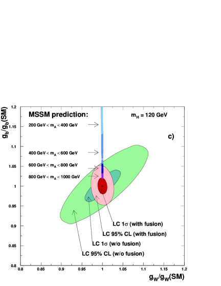
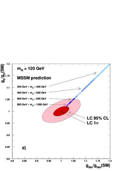
Figure 12: Higgs boson coupling determinations at TESLA, for $M_{H}=120$ GeV with 500 fb^-1 of data, and the expected deviations in the MSSM; from Ref. [7].

5. Conclusions

In the SM, global fits of the electroweak data favour a light Higgs boson, $M_{H}\raisebox{-3.69899pt}{~{}\shortstack{$<$ \\ [-0.07cm] $\sim$}}~{}200$ GeV; if the theory is to remain valid up to the GUT scale, the Higgs boson should be lighter than $200$ GeV. In supersymmetric extensions of the SM, there is always one light Higgs boson with a mass $M_{h}\raisebox{-3.69899pt}{~{}\shortstack{$<$ \\ [-0.07cm] $\sim$}}~{}130$ GeV in the minimal version [and $M_{h}\raisebox{-3.69899pt}{~{}\shortstack{$<$ \\ [-0.07cm] $\sim$}}~{}200$ GeV in more general extensions]. Thus, a Higgs boson is definitely accessible to the next generation of experiments. The heavier Higgs bosons are expected to have masses in the range of the electroweak symmetry breaking scale and can be probed as well.

The detection of a Higgs particle is possible at the upgraded Tevatron for $M_{H}\raisebox{-3.69899pt}{~{}\shortstack{$<$ \\ [-0.07cm] $\sim$}}~{}130$ GeV and is not a problem at the LHC where even much heavier Higgs bosons can be probed: in the SM up to $M_{H}\sim 1$ TeV and in the MSSM for $M_{A,H,H^{\pm}}$ of order a few hundred GeV, depending on $\tan\beta$. Relatively light Higgs bosons can also be found at future $e^{+}e^{-}$ colliders with c.m. energies $\sqrt{s}\raisebox{-3.69899pt}{~{}\shortstack{$>$ \\ [-0.07cm] $\sim$}}~{}350$ GeV; the signals are very clear, and the expected high luminosity allows a thorough investigation of their fundamental properties.

In fact, a very important issue once Higgs particles are found, will be to probe in all its facets the electroweak symmetry breaking mechanism. In many aspects, the searches and tests at future $e^{+}e^{-}$ colliders are complementary to those that will be performed at the LHC. An example can be given in the context of the MSSM.

In constrained scenarios, such as the minimal supergravity model, the heavier $H,A$ and $H^{\pm}$ bosons tend to have masses of the order of several hundred GeV and therefore will escape detection at both the LHC and linear collider. The right–handed panel of Fig. 1 shows the number of Higgs particles in the $(M_{A},\tan\beta$) plane, which can observed at the LHC and in the white area, only the lightest $h$ boson can be observed. In this parameter range, the $h$ boson couplings to fermions and gauge bosons will be almost SM–like and, because of the relatively poor accuracy of the measurements at the LHC, it would be difficult to resolve between the SM and MSSM (or extended) scenarios. At $e^{+}e^{-}$ colliders such as TESLA, the Higgs couplings can be measured with a great accuracy, allowing a distinction between the SM and the MSSM Higgs boson to be made close to the decoupling limit, i.e. for pseudoscalar boson masses, which are not accessible at the LHC. This is exemplified in Fig. 12, where the accuracy in the determination of the Higgs couplings to $b\bar{b},\tau^{+}\tau^{-}$ and $WW$ are displayed, together with the predicted values in the MSSM for different values of $M_{A}$. The two scenarios can be distinguished for pseudoscalar Higgs masses up to 1 TeV and, thus, beyond the LHC reach.

Acknowledgements: I thank the organizers of the Conference, in particular S. Banerjee, D.P. Roy and K. Sridhar, for the invitation to the meeting and for the very nice and warm atmosphere. I would also like to express all my sympathy to D.P. Roy for the tragedy he has to bear.

References

- [1] For a review on the Higgs sector in the SM and MSSM, see: J. Gunion, H. Haber, G. Kane and S. Dawson, “The Higgs Hunter’s Guide”, Addison–Wesley, Reading 1990.
- [2] M. Carena et al., Higgs WG report for “RUN II at the Tevatron”, hep-ph/0010338.
- [3] Proceedings of the Les Houches Workshops on “Physics at TeV Colliders”: A. Djouadi et al., hep-ph/0002258 (1999) and D. Cavalli et al., hep-ph/0203056 (2001).
-
[4]
CMS Collaboration, Technical Proposal, Report CERN/LHCC/94-38
(1994);
ATLAS Collaboration, Technical Design Report, CERN/LHCC/99-15 (1999). - [5] M. Dittmar, Talk given at WHEPP 1999, Pramana 55 (2000) 151; F. Gianotti, talk given at the LHC Committee Meeting, CERN, 5/7/2000.
- [6] E. Accomando, Phys. Rept. 299 (1998) 1; American Lin. Col. WG (T. Abe et al.), hep-ex/0106057; ACFA Lin. Col. Higgs WG (S. Kiyoura et al.), hep-ph/0301172.
- [7] TESLA Technical Design Report, Part III, DESY–01–011C, hep-ph/0106315.
- [8] J. Gunion, these proceedings.
- [9] The LEP Higgs Working Group, Note/2002-01 for the SM and Note/2002-04 for the MSSM. See also, the summary of P. Igo–Kemenes at this conference.
- [10] The LEP and SLD Electroweak Working Group, LEPEWW/2002-02 (Dec. 2002), hep-ex/0212036. See also G. Altarelli, talk given at this conference.
- [11] B. Lee, C. Quigg and H. Thacker, Phys. Rev. 16 (1977) 1519. For a recent discusion see, A. Arhrib, hep-ph/0012353.
- [12] Recent analyses: T. Hambye and K. Riesselman, Phys. Rev. D55 (1997) 7255; C. Kolda and H. Murayama, JHEP 0007 (2000) 035; G. Isidori, G. Ridolfi, A. Strumia, Nucl. Phys. B609 (2001) 387; K. Tobe and J. Wells, Phys. Rev. D66 (2002) 013010.
- [13] For recent reviews and calculations up to , see: M. Carena et al., Nucl. Phys. B580 (2000) 29; J.R. Espinosa and R.J. Zhang, Nucl. Phys. B586 (2000) 3.
- [14] A. Brignole, G. Degrassi, P. Slavich and F. Zwirner, Nucl. Phys. B611 (2001) 403, B631 (2002) 195 and B643 (2002) 79; A. Dedes and P. Slavich, hep-ph/0212132.
- [15] B.C. Allanach (SOFTSUSY), hep-ph/0104145; A. Djouadi, J.L. Kneur and G. Moultaka (SuSpect), hep-ph/0211331; W. Porod (SPHENO), hep-ph/0301101.
- [16] For details on decays in the SM and MSSM, see: A. Djouadi, M. Spira and P. M. Zerwas, Z. Phys. C70 (1996) 427; A. Djouadi, J. Kalinowski and P. M. Zerwas, Z. Phys. C70 (1996) 435; A. Djouadi and P. Gambino, Phys. Rev. D51 (1995) 218.
- [17] See, e.g. : A. Djouadi et al., Phys. Lett. B376 (1996) 220; M. Bisset, M. Guchait and S. Moretti, Eur. Phys. J. C19 (2001) 143; F. Moortgat, hep-ph/0105081.
- [18] For some analyses, see: J.I. Illana et al., Eur. Phys. J.C1 (1998) 149; A. Djouadi, Phys. Lett. B435 (1998) 101; G. Bélanger et al., Nucl. Phys. B581 (2000) 3.
- [19] A. Djouadi, J. Kalinowski and M. Spira, Comput. Phys. Commun. 108 (1998) 56.
- [20] The original papers are: H. Georgi et al., Phys. Rev. Lett. 40 (1978) 692; S.L. Glashow, D.V. Nanopoulos and A. Yildiz, Phys. Rev. D18 (1978) 1724; R.N. Cahn and S. Dawson, Phys. Lett. B136 (1984) 196; K. Hikasa, Phys. Lett. B164 (1985) 341; G. Altarelli, B. Mele and F. Pitolli, Nucl. Phys. B287 (1987) 205; Z. Kunszt, Nucl. Phys. B247 (1984) 339; J. Gunion, Phys. Lett. B253 (1991) 269.
- [21] M. Spira, hep-ph/9711394 and hep-ph/9810289.
- [22] A. Djouadi, M. Spira and P. Zerwas, Phys. Lett. B264 (1991) 440; S. Dawson, Nucl. Phys. B359 (1991) 283; M. Spira et al., Nucl. Phys. B453 (1995) 17; Phys. Lett. B318 (1993) 347; S. Dawson, A. Djouadi, M. Spira, Phys. Rev. Lett. 77 (1996) 16.
- [23] R.V. Harlander and W. Kilgore, Phys. Rev. Lett. 88 (2002) 201801; C. Anastasiou and K. Melnikov, Nucl. Phys. B646 (2002) 220.
- [24] V. Ravindran, J. Smith and W.L. Van Neerven, Nucl. Phys. B634 (2002) 247; D. de Florian, M. Grazzini and Z. Kunszt, Phys. Rev. Lett. 82 (1999) 5209.
- [25] T. Han, G. Valencia and S. Willenbrock, Phys. Rev. Lett. 69 (1992) 3274; D.A. Dicus and S. Willenbrock, Phys. Rev. D39 (1989) 751; A. Djouadi and M. Spira, Phys. Rev. D62 (2000) 014004.
- [26] R. Godbole et al., in preparation. For earlier work, see: D.P. Roy, hep-ph/9404304; D. Choudhury and D.P. Roy, Phys. Lett. B322 (1994) 368.
- [27] V. Barger et al., Phys. Rev. D44 (1991) 1426; V. Barger, R. Phillips, D. Zeppenfeld, Phys. Lett. B346 (1995) 106; D. Rainwater and D. Zeppenfeld JHEP 9712 (1997) 5.
- [28] D. Zeppenfeld, R. Kinnunen, A. Nikitenko and E. Richter-Was, Phys. Rev. D62 (2000) 013009.
- [29] T. Plehn, D. Rainwater and D. Zeppenfeld, Phys. Rev. D61 (2000) 093005; O. Eboli and D. Zeppenfeld, Phys. Lett. B495 (2000) 147; N. Kauer, T. Plehn, Rainwater and D. Zeppenfeld, Phys. Lett. B503 (2001) 113; T. Plehn and D. Rainwater, Phys. Lett. B520 (2001) 108; M.L. Mangano et al., Phys. Lett. B556 (2003) 50. See also T. Han and B. McElrath Phys. Lett. B528 (2002) 81, for .
- [30] K. Jacobs and collaborators, talks given during the ATLAS week, February 2003.
-
[31]
W. Beenakker et al., Phys. Rev. Lett. 87 (2001) 201805
and hep-ph/0211352;
S. Dawson et al., Phys. Rev. Lett. 87 (2001) 201804 and hep-ph/0211438. - [32] S.Y. Choi, D.J. Miller, M.M. Muhlleitner and P.M. Zerwas, Phys. Lett. B553 (2003) 61; V. Barger et al., Phys. Rev. D49 (1994) 79.
- [33] A. Bawa, C. Kim and A. Martin, Z. Phys. C47 (1990) 75; V. Barger, R. Phillips and D.P. Roy, Phys. Lett. B324 (1994) 236; S. Moretti and K. Odagiri, Phys. Rev. D55 (1997) 5627; J. Gunion, Phys. Lett. B322 (1994) 125; F. Borzumati, J.L. Kneur and N. Polonsky, Phys. Rev. D60 (1999) 115011; D. Miller, S. Moretti, D.P. Roy and W. Stirling, Phys. Rev. D61 (2000) 055011; D.P. Roy, Phys. Lett. B459 (1999) 607.
- [34] E. Boos et al, Phys. Rev. D66 (2002) 055004.
- [35] Aseshkrishna Datta et al., Phys. Rev. D65 (2002) 015007 and hep-ph/0303095
- [36] J. Ellis, M. Gaillard and D. Nanopoulos, Nucl. Phys. B106 (1976) 292; B. Lee, C. Quigg and H. Thacker, Phys. Rev. D16 (1977) 1519; J.D. Bjorken, SLAC Report 198 (1976); B. Ioffe and V. Khoze, Sov. J. Part. Nucl. 9 (1978) 50; D. Jones and S. Petcov, Phys. Lett. B84 (1979) 440; R. Cahn and S. Dawson in [20], G. Altarelli, B. Mele and F. Pitolli in [20], W. Kilian, M. Krämer and P.M. Zerwas, Phys. Lett. B373 (1996) 135; A. Djouadi, J. Kalinowski and P. M. Zerwas, Mod. Phys. Lett. A7 (1992) 1765 and Z. Phys. C54 (1992) 255; G. Gounaris, D. Schildknecht and F. Renard, Phys. Lett. B83 (1979) 191; M. Muhlleitner et al., Eur. Phys. J.C10 (1999) 27.
- [37] J. Fleischer and F. Jegerlehner, Nucl.Phys.B216 (1983) 469; B. Kniehl, Z.Phys.C55 (1992) 605; A. Denner, J. Kublbeck, R. Mertig, M. Bohm, Z.Phys.C56 (1992) 261.
- [38] G. Bélanger et al., hep-ph/0212261 and hep-ph/0211268; A. Denner, S. Dittmaier, M. Roth and M. Weber, hep-ph/0302198 and hep-ph/0301189.
- [39] J. Ellis et al., Phys. Rev. D39 (1989) 844; A. Djouadi et al., Z. Phys. C57 (1993) 569 and Z. Phys. C74 (1997) 93.
- [40] J.F. Gunion et al., hep-ph/0112334; see also J.F. Gunion, these proceedings.