Chromofields of Strings and Baryons

Abstract

We calculate color electric fields of quark/antiquark ($\bar{q}q$) and 3 quark ($qqq$) systems within the chromodielectric model (CDM). We explicitly evaluate the string tension of flux tubes in the $\bar{q}q$–system and analyze their profile. To reproduce results of lattice calculations we use a bag pressure $B=(320\mbox{MeV})^{4}$ from which an effective strong coupling constant $\alpha_{s}\approx 0.3$ follows. With these parameters we get a $Y$ shaped configuration for large $qqq$–systems.

1 Introduction

Quantum chromodynamics (QCD) is the widely accepted theory for the dynamics of quarks and gluons. Despite its success in the regime of high momemtum transfer it remains an outstanding task to explain the low energy behavior of hadrons within QCD. Only in the last 10 years lattice QCD (lQCD) has found detailed evidence for the confinement of quarks in hadrons Bali:2000gf but it still fails to give a dynamical description of this phenomenon. It is therefore necessary to rely on models, capable to describe confinement dynamically on the one hand and to reproduce static results of lQCD on the other hand.

In this talk we present static calculations within the Chromodielectric Model Friedberg:1977eg ; Friedberg:1977xf ; Traxler:1998bk , namely the detailed analysis of quark–antiquark strings and three–quark configurations.

2 Phenomenology of the Model

In the Chromodielectric Model (CDM) it is assumed, that the vacuum of QCD behaves in the long range limit as a perfect color dielectric medium with vanishing dielectric constant $\kappa=0$. The medium is generated through the non-abelian part of the gluonic sector of QCD which is represented in CDM as a scalar color singlet field $\sigma$. The remaining two abelian gluon fields are able to propagate through this medium. The scalar field $\sigma$ is driven by a scalar potential $U(\sigma)$ (see fig. 1) which exhibits two (quasi) stable points, separating the non-perturbative, perfect dielectric phase where $\sigma=\sigma_{{\mbox{\scriptsize vac}}}$, from the perturbative phase with $\kappa=1$, where the color fields can propagate freely and $\sigma=0$.

In our description quarks are treated classically and the gluons are coupled to the quark current $j^{\mu,a}$. This results in the following Lagrangian

$${\cal L} = {\cal L}_{q}+{\cal L}_{g}+{\cal L}_{\sigma}$$ (1)

$${\cal L}_{q} = -\sum\limits_{k}m_{k}\sqrt{1-\dot{\vec{x}}_{k}^{2}}\;w\left(\vec{x}-\vec{x}_{k}(t)\right)$$

$$-g_{s}\;j_{\mu}^{a}\,A^{\mu,a}$$

$${\cal L}_{g} = -{\textstyle\frac{1}{4}}{\kappa(\sigma)}F_{\mu\nu}^{a}F^{\mu\nu,{a}}$$ (3)

$${\cal L}_{\sigma} = {{\textstyle\frac{1}{2}}\partial_{\mu}\sigma\partial^{\mu}\sigma-U(\sigma)}$$ (4)

$$F^{\mu\nu,{a}} = \partial^{\mu}A^{\nu,a}-\partial^{\nu}A^{\mu,a},\;\;\;a\in\{3,8\}$$ (5)

$$j^{\mu,a} = \sum\limits_{k}q_{k}^{a}\;u_{k}^{\mu}\;w\left(\vec{x}-\vec{x}_{k}(t)\right)=(\rho^{a},\vec{\jmath}^{\;a})$$ (6)

with $u_{k}^{\mu}$ being the 4-velocity of particle $k$ with classical charge $q_{k}^{a}$ (see fig. 1) and extension $w\left(\vec{x}-\vec{x}_{k}(t)\right)$. The scalar potential $U(\sigma)$ is chosen to be of a quartic form and is shown in fig. 1. In this work $U(\sigma)$ has no relative maximum between $\sigma=\sigma_{{\mbox{\scriptsize vac}}}$ and $\sigma=0$ and $U$ is determined through the bag pressure $B=U(0)$ and $\sigma_{{\mbox{\scriptsize vac}}}$ alone. The dielectric function is of the form $\kappa(\sigma)=\exp\left(-\frac{\sigma^{3}}{\sigma_{0}^{3}}\right)$ for $\sigma\geq 0$ and $\kappa(\sigma)=1$ else and has $\kappa(\sigma_{{\mbox{\scriptsize vac}}})\equiv\kappa_{{\mbox{\scriptsize vac}}}\ll 1$.

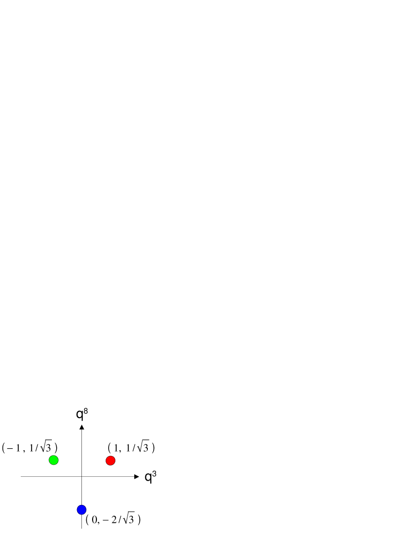
Figure 1: Left: The color charges of the green (left), red (right) and blue (lower) quark. Right: The dielectric function $\kappa(\sigma)$ (dashed) and the scalar potential $U(\sigma)$.

In the static case, the equations of motion for the electric potentials $\Phi^{a}$ and for the confinement field $\sigma$ following from eq. (1) are:

$$\vec{\nabla}\cdot\left(\kappa(\sigma)\,\vec{\nabla}\Phi^{a}\right)=-g_{s}\;\rho^{a}$$ (7)

and

$$\nabla^{2}\sigma=U^{\prime}(\sigma)-{\textstyle\frac{1}{2}\frac{\kappa^{\prime}(\sigma)}{\kappa(\sigma)^{2}}}\left(\vec{D^{3}}\cdot\vec{D^{3}}+\vec{D^{8}}\cdot\vec{D^{8}}\right),$$ (8)

where $\vec{D^{a}}=\kappa(\sigma)\vec{\nabla}\Phi^{a}$ denotes the color electric displacement. The energy (neglecting quark masses) is given by:

$$E = E_{\sigma}+E_{g}$$ (9)

$$E_{\sigma} = \int\left({\textstyle\frac{1}{2}}(\nabla\sigma)^{2}+U(\sigma)\right)d^{3}r$$ (10)

$$E_{g} = \frac{1}{2}\int\left(\vec{E^{3}}\cdot\vec{D^{3}}+\vec{E^{8}}\cdot\vec{D^{8}}\right)d^{3}r\equiv\int\varepsilon_{g}\,d^{3}r.$$ (11)

Confinement of color fields in our model is achieved by means of Gauss’s law in eq. (7) and the characteristic form of the dielectric function $\kappa(\sigma)$: A single colored quark would generate a spherical electric field. In the vicinity of the quark the field is strong enough to push the confinement field from $\sigma=\sigma_{{\mbox{\scriptsize vac}}}$ towards smaller values and forms a cavity in the surrounding vacuum. As $\kappa(\sigma)$ drops to zero at the boundary of the cavity, the electric field $\vec{E^{a}}=\frac{\vec{D^{a}}}{\kappa(\sigma)}$ diverges and so does the electric field energy (11). Note that in this version of CDM there is no direct coupling between the quarks and the confinement field as proposed in Friedberg:1977eg ; Schuh:1986mi .

3 $\bar{q}q$ Strings

In contrast to configurations with net color, all white configurations have finite energy and color fields are confined into well defined spatial regions. Again, eq. (7) enforces an electric color field, but field lines now end on the anti–color and are parallel to the boundary of the cavity. In this case the color electric displacement is suppressed with the dielectric constant in the non-perturbative vacuum. Both the electric field energy and the confinement field energy are negligible in the outside.

In this section we study the field configurations of color flux tubes stretching from a quark $q$ to an antiquark $\bar{q}$. We start by showing the electric field $\vec{E^{3}}$ and $\vec{D^{3}}$ in fig. 2.

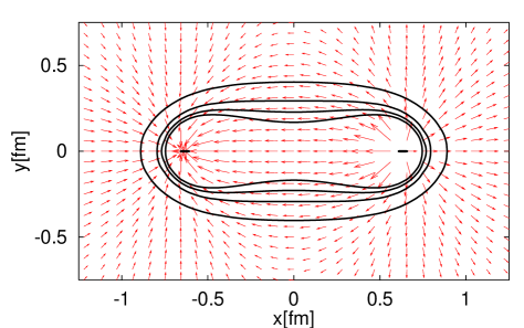
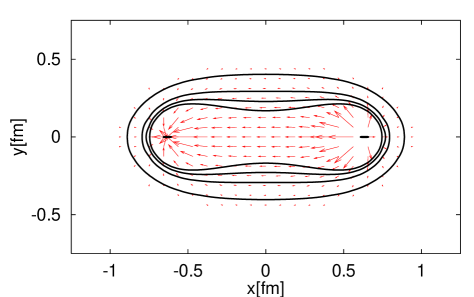
Figure 2: The color fields $\vec{E^{3}}$ (upper panel) and $\vec{D^{3}}$ (lower panel). The contour lines give the electric energy density (11) $\varepsilon_{g}=1,3,5,7$ fm^-4 from the outside. Only the electric displacement $\vec{D^{a}}$ is confined to the flux tube.

It is seen that the electric displacement vanishes outside the cavity. The flux tube can be characterized by the profile function, i. e. the component of $\vec{D}$ parallel to the string axis along the center line perpendicular to the string axis. This profile has been studied within lQCD in Bali:1995de . The profile depends mainly on the choice of $U(\sigma)$, i. e. on the bag constant $B$ and the vacuum value $\sigma_{{\mbox{\scriptsize vac}}}$ as shown in fig. 3. The bag constant acts as a pressure against the electric field and therefore an increasing $B$ leads to decreasing width of the profile. In order to fulfill Gauss’s law (7) the electric $\vec{D}$ field on the string axis must increase with increasing $B$.

The value of $\sigma_{{\mbox{\scriptsize vac}}}$ controls the surface of the bag. Decreasing its value leads to a sharper surface. In our simulations the detailed form of the dielectric function (see fig. 1) has little effect on the profile.

Figure 3: The string profile of a $1.2$ fm string. Increasing the bag pressure $B$ decreases the width and simultanously increases the maximal value of the $\vec{D}$ field (left) and increasing $\sigma_{{\mbox{\scriptsize vac}}}$ smoothes the surface (right). All constant parameters are taken from tab. 1.

With the parameters given in tab. 1 we reproduce the results of lQCD Bali:2000gf ; Bali:1995de as can be seen in fig. 4.

$B^{\frac{1}{4}}$	$\sigma_{{\mbox{\scriptsize vac}}}$	$\kappa_{{\mbox{\scriptsize vac}}}$	$g_{s}$
$320$MeV	$1.5$fm-1	0.01	1.0

Table 1: Model parameters used in this work.

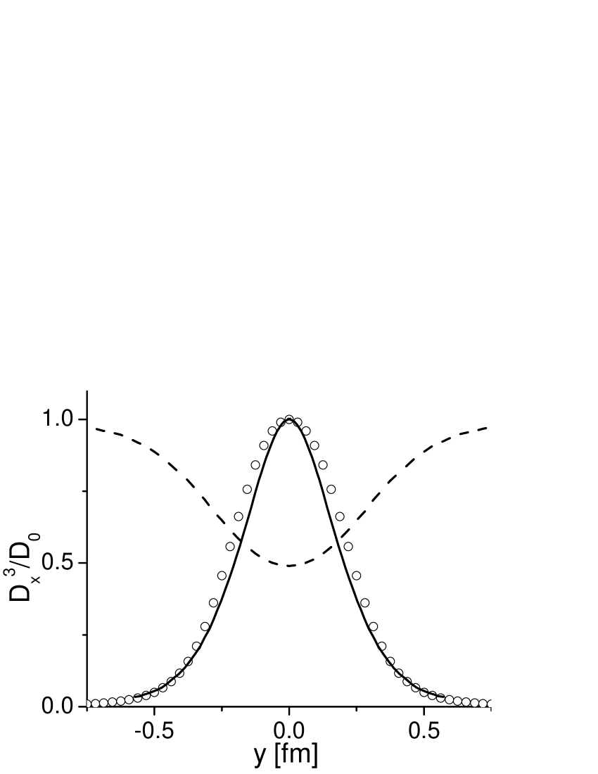
Figure 4: Left: The string profile within CDM (circles) compared to lQCD results (solid line) Bali:2000gf . The confinement field (dashed line) drops to $\sigma\approx 0.5\sigma_{{\mbox{\scriptsize vac}}}$ inside the string. Right: The string potential within CDM (squares) and a fit to the Cornell potential (12). The first two data points are not included in the fit as the Coulomb potential does not hold for too small distances due to finite extension of the charges with rms radius $\sqrt{\langle\vec{r}^{2}\rangle}\approx 0.1$ fm.

Using the same parameters we can calculate the string tension of the flux tube. We vary the $q$-$\bar{q}$ distance $r$ and plot the total energy of eq. (9) as a function of $r$ in fig. 4. For $r>0.5$ fm the energy rises linearly. We fit our results to a Cornell potential

$$E_{c}(r)=E_{0}+\tau r-\frac{\alpha_{{\mbox{\scriptsize eff}}}}{r},$$ (12)

where the linear term reflects the confinement behavior for large $\bar{q}q$-separations and the Coulomb term describes the one gluon exchange dominant at small $r$. The constant term $E_{0}=560$ MeV is due to electric self energies included in eq. (11). We find a string tension $\tau=988$ MeV/fm and a value $\alpha_{{\mbox{\scriptsize eff}}}=0.291$ which is to be compared to lQCD results where $\alpha_{{\mbox{\scriptsize eff}}}=0.295$ Bali:2000gf . It should be noted, that due to the high bag pressure $B$ the electric fields are not strong enough to expel totally the non-perturbative vacuum out of the string. The confinement field only drops to $\sigma\approx 0.5\sigma_{\mbox{\scriptsize vac}}$, i. e. the dielectric function rises to $\kappa\approx 0.5$. However, confinement is still achieved as the energy of the color fields does not leak into the outside.

4 Baryons

In this section we study color fields of baryon like $qqq$–configurations. Given that the energy scales linearly with the $\bar{q}q$-separation, one can argue that configurations with 3 quarks sitting on the corner of an equilateral triangle will form strings with minimal total string length. This would be a configuration with a central Steiner point, called a $Y$ configuration. However, if only two quark interactions are dominant, one might expect strings stretching pairwise from one quark to another, which would be the $\Delta$ configuration. In lQCD the $qqq$ potential has been studied and there are indications for both the $\Delta$ baryon Bali:2000gf ; Alexandrou:2001ip and the $Y$ baryon Takahashi:2002bw . However in the Gaussian Stochastic Vacuum model Kuzmenko:2000rt clear evidence for the $Y$ ansatz is found.

In fig. 5 we plot the electric field distribution for the baryon with the parameters given in tab. 1. The quarks are separated a distance $\ell=0.7(1.3)$ fm from the Steiner point, i.e.  the $qq$ distance is $L=\sqrt{3}\ell\approx 1.2(1.7)$ fm.

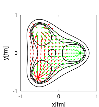
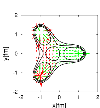
Figure 5: The color fields of a $qqq$ configuration with $\ell=0.7$($1.3$) fm left (right). The contour lines correspond to $\varepsilon_{g}=1,3,5,7$ fm^-4 (left) and $\varepsilon_{g}=1,1.4,1.8$ fm^-4 (right).

The field is clearly different from a simple superposition of 3 flux tubes between the quarks (see fig. 2). The electric energy is pushed towards the center of the baryon, and a $Y$ shaped configuration (at least for large quark separations) is seen.

5 Summary

We have analyzed the $\bar{q}q$ string within CDM and have reproduced the geometric profile function as well as the potential. With a bag constant $B=(320\,\mbox{MeV})^{4}$ and $\sigma_{{\mbox{\scriptsize vac}}}=1.5$ fm^-1 we get a string tension $\tau=988$ MeV/fm and an effective strong coupling $\alpha_{{\mbox{\scriptsize eff}}}=0.29$. $qqq$ configurations with large $qq$ separations tend to show a $Y$ shaped geometry.

References

- (1) G. S. Bali, Phys. Rept. 343 (2001) 1–136.
- (2) R. Friedberg and T. D. Lee, Phys. Rev. D15 (1977) 1694.
- (3) R. Friedberg and T. D. Lee, Phys. Rev. D16 (1977) 1096.
- (4) C. T. Traxler, U. Mosel, and T. S. Biro, Phys. Rev. C59 (1999) 1620–1636.
- (5) A. Schuh, H. J. Pirner, and L. Wilets, Phys. Lett. B174 (1986) 10–14.
- (6) G. S. Bali, K. Schilling, and C. Schlichter, Phys. Rev. D51 (1995) 5165–5198.
- (7) C. Alexandrou, P. De Forcrand, and A. Tsapalis, Phys. Rev. D65 (2002) 054503.
- (8) T. T. Takahashi, H. Suganuma, Y. Nemoto, and H. Matsufuru, Phys. Rev. D65 (2002) 114509.
- (9) D. S. Kuzmenko and Y. A. Simonov, Phys. Atom. Nucl. 64 (2001) 107–119.