Abstract

Two-loop corrections for the form factor in a massive Abelian theory are evaluated, which result from the insertion of massless fermion or scalar loops into the massive gauge boson propagator. The result is valid for arbitrary energies and gauge boson mass. Power-suppressed terms vanish rapidly in the high energy region where the result is well approximated by a polynomial of third order in $\ln(s/M^{2})$. The relative importance of subleading logarithms is emphasised.

PACS numbers: 12.38.Bx, 12.38.Cy, 12.15.Lk

1 Introduction

One of the central tasks of the next generation of high energy colliders – the Large Hadron Collider presently under construction or projects under consideration like TESLA – will be the exploration of electroweak interactions at ultrahigh energies: in the TeV region or beyond. The control of radiative corrections plays an essential role in this context. Important differences arise in their structure when comparing low energies, say up to ${\cal O}(M_{W,Z})$, with this ultrahigh energy region. In the first case gauge boson self energies play the dominant role, with contributions from virtual top quarks or Higgs bosons as most prominent examples. At high energies, however, large logarithms arising from virtual gauge boson exchange become increasingly important. The leading terms of order $(\alpha_{\rm weak}/4\pi)^{n}\ln^{2n}(s/M^{2})$, often denoted Sudakov logarithms, could easily affect the cross section by 10% or more once the energy reaches one or two TeV. In principle these and even subleading terms have to be summed to all orders. In practice, in view of the smallness of the weak coupling, it is often sufficient to restrict the discussion to terms up to order $\alpha_{\rm weak}^{2}$. (For recent discussions of electroweak Sudakov logarithms see e.g. [1, 2, 3, 4].)

At present, not only leading logarithms have been evaluated [5, 6], using arguments originally developed in the context of QCD, next-to-leading (NLL, [7, 8]) and even next-to-next-to-leading (NNLL, [9]) logarithmic corrections have been calculated for four-fermion processes. Numerically these subleading terms are large and mostly of alternating sign. To arrive at reliable predictions, say at the level of ${\cal O}$(1%), the evaluation of all two-loop non-power-suppressed corrections for four-fermion processes seems desirable. Furthermore it seems useful to test the basic assumption of this approach that power-suppressed terms of order $M^{2}/s$ can be neglected.

At the moment this program is completely out of reach, as far as four-fermion processes in the complete electroweak theory are concerned, and even in the context of a simplified version like a spontaneously broken $SU(2)$ gauge theory or an Abelian theory with a massive gauge boson this seems like an extremely difficult task. In this present paper we therefore consider a simpler two-loop problem which nevertheless encompasses already many aspects of the complete calculation: The contributions from loops of massless fermions or scalars to the vertex function in an Abelian theory with a massive gauge boson, which already exhibits many features characteristic for the complete problem.

The result will be presented for arbitrary $s/M^{2}$. This allows to investigate the complete series in the logarithmic expansion as well as power-suppressed terms. In the next section we briefly recall the results for the form factor obtained in [7, 8, 9] and introduce our notation. In section 3 we present the main results of this paper and discuss its implications. Section 4 contains our summary and conclusions.

2 The Abelian form factor

Let us begin with a discussion of the form factor for the vector current in an Abelian gauge theory with a massive gauge boson and massless fermions in the Sudakov limit. In Born approximation, one writes

$${\cal F}_{B}=\bar{\psi}(p_{2})\gamma_{\mu}\psi(p_{1}),$$ (1)

and we study the limit $s=(p_{1}-p_{2})^{2}\to-\infty$ with on-shell massless fermions, $p_{1}^{2}=p_{2}^{2}=0$, and massive gauge bosons, $M^{2}\ll-s$. For convenience we choose $p_{1,2}=(Q/2,0,0,\mp Q/2)$ so that $2p_{1}\!\cdot\!p_{2}=Q^{2}=-s$ and limit the discussion to the spacelike region. The transition to timelike momentum transfer is easily accomplished through analytic continuation.

The large logarithmic corrections in the Sudakov limit can be resummed to all orders of perturbation theory [10, 11], such that the asymptotic behaviour of the form factor is obtained from

$${\cal F}=F_{0}(\alpha(M^{2}))\exp\left\{\int_{M^{2}}^{Q^{2}}\frac{{\rm d}x}{x}\left[\int_{M^{2}}^{x}\frac{{\rm d}x^{\prime}}{x^{\prime}}\gamma(\alpha(x^{\prime}))+\zeta(\alpha(x))+\xi(\alpha(M^{2}))\right]\right\}{\cal F}_{B}.$$ (2)

The next-to-next-to-leading logarithmic corrections include all the terms of the form $\alpha^{n}\log^{2n-m}(Q^{2}/M^{2})$ with $m=0,~{}1,~{}2$. To this accuracy, one needs for the anomalous dimensions $\gamma$, $\zeta$ and $\xi$ in Eq. (2) the one-loop results

$$\gamma^{(1)}=-2C_{F}\,,\quad\zeta^{(1)}=3C_{F}\,,\quad\xi^{(1)}=0\,,\quad F_{0}^{(1)}=-C_{F}\left(\frac{2}{3}\pi^{2}+\frac{7}{2}\right),$$ (3)

as well as the two-loop result for the anomalous dimension $\gamma^{(2)}$. Here we define $\gamma=\sum_{n}\left(\frac{\alpha}{4\pi}\right)^{n}\gamma^{(n)}$ and similarly for $\zeta$, $\xi$ and $F_{0}$. An efficient strategy for the evaluation of the anomalous dimensions listed in Eq. (3) which was based on the expansion by regions has been described in [7]. In the $\overline{\rm MS}$-scheme, including $n_{f}$ light fermions and $n_{s}$ light scalars in the fundamental representation, $\gamma^{(2)}$ reads [12, 13, 14]

$$\gamma^{(2)}=-2C_{F}\left[\left(-\frac{\pi^{2}}{3}+\frac{67}{9}\right)C_{A}-\frac{20}{9}T_{F}n_{f}-\frac{8}{9}T_{F}n_{s}\right].$$ (4)

The result for the form factor, up to ${\cal O}(\alpha^{2})$, is written in the following form:

$${\cal F}={\cal F}_{B}+\frac{\alpha}{4\pi}\,{\cal F}^{(1)}+\left(\frac{\alpha}{4\pi}\right)^{2}\,{\cal F}^{(2)}$$ (5)

with

$${\cal F}^{(1)}=\left\{\frac{1}{2}\gamma^{(1)}\ln^{2}\left(\frac{Q^{2}}{M^{2}}\right)+\left(\zeta^{(1)}+\xi^{(1)}\right)\ln\left(\frac{Q^{2}}{M^{2}}\right)+F_{0}^{(1)}\right\}{\cal F}_{B}$$ (6)

and $\alpha=\alpha_{\overline{\rm MS}}(M^{2})$. To obtain ${\cal F}^{(2)}$, one expands Eq. (2) for the form factor at two loops up to next-to-next-to-next-to-leading logarithmic (N³LL) accuracy,

$${\cal F}^{(2)}_{\rm LL} =\frac{1}{8}\big{(}\gamma^{(1)}\big{)}^{2}\ln^{4}\left(\frac{Q^{2}}{M^{2}}\right){\cal F}_{B},$$ (7)

$${\cal F}^{(2)}_{\rm NLL} =\frac{1}{2}\left(\zeta^{(1)}-\frac{1}{3}\beta_{0}\right)\gamma^{(1)}\ln^{3}\left(\frac{Q^{2}}{M^{2}}\right){\cal F}_{B},$$ (8)

$${\cal F}^{(2)}_{\rm NNLL} =\frac{1}{2}\biggl{(}\gamma^{(2)}+\big{(}\zeta^{(1)}-\beta_{0}\big{)}\zeta^{(1)}+F_{0}^{(1)}\gamma^{(1)}\biggr{)}\ln^{2}\left(\frac{Q^{2}}{M^{2}}\right){\cal F}_{B},$$ (9)

$${\cal F}^{(2)}_{\rm N^{3}LL} =\left(\zeta^{(2)}+\xi^{(2)}+F_{0}^{(1)}\zeta^{(1)}\right)\ln\left(\frac{Q^{2}}{M^{2}}\right){\cal F}_{B},$$ (10)

where $\xi^{(1)}=0$ has been omitted.

Employing the results of Eqs. (3) and (4), we see a particular pattern of growing coefficients of the logarithms which reflects the general structure of logarithmically enhanced electroweak corrections. For an Abelian theory ($C_{F}=1$, $T_{F}=1$, $C_{A}=0$),

$${\cal F}^{(1)} =\biggl{\{}-\ln^{2}\left(\frac{Q^{2}}{M^{2}}\right)+3\ln\left(\frac{Q^{2}}{M^{2}}\right)-\left(\frac{2}{3}\pi^{2}+\frac{7}{2}\right)\biggr{\}}{\cal F}_{B}\,,$$ (11)

$${\cal F}^{(2)} =\biggl{\{}\frac{1}{2}\ln^{4}\left(\frac{Q^{2}}{M^{2}}\right)-\left(\frac{4}{9}n_{f}+\frac{1}{9}n_{s}+3\right)\ln^{3}\left(\frac{Q^{2}}{M^{2}}\right)$$

$$\qquad\qquad\qquad{}+\left(\frac{38}{9}n_{f}+\frac{25}{18}n_{s}+\frac{2}{3}\pi^{2}+8\right)\ln^{2}\left(\frac{Q^{2}}{M^{2}}\right)\biggr{\}}{\cal F}_{B}$$ (12)

to NNLL accuracy. The relatively small coefficient of the leading logarithm and the large coefficient of the NNLL term in the form factor are clearly indicative of the importance of subleading logarithmic corrections. At N³LL accuracy, the still unknown quantities $\zeta^{(2)}$ and $\xi^{(2)}$ enter.

3 Fermionic and scalar contributions at two loops

As stated in the introduction, the evaluation of all two-loop terms linear in the logarithm or even of the two-loop constant terms is desirable. As a first step, and as a new result, the corrections due to $n_{f}$ massless fermions and $n_{s}$ charged massless scalars have been calculated for the Abelian form factor. These fermionic and scalar corrections are separately gauge invariant and renormalisable. In two loops, they give contributions proportional to $n_{f}$ and $n_{s}$ respectively.

To calculate these terms, the two-loop diagrams depicted in Fig. 1 and the gauge boson mass renormalisation have been evaluated.

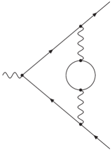
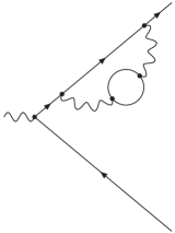
Figure 1: Two-loop diagrams contributing to the fermionic and scalar form factor. The circle represents a fermion loop for the $n_{f}$-part or a scalar loop for the $n_{s}$-part of the form factor.

This calculation was done using dimensional regularisation. Due to the simple topologies of the diagrams in Fig. 1, the integration corresponding to the insertion of the fermion or scalar loop can be done first, leaving only one-loop integrals with an additional massless propagator of non-integer power. Tensor integrals were reduced to scalar ones by employing the method developed by Passarino and Veltman [15]. After using partial integration for further reduction, we were left with only three master integrals which could be calculated with the help of Feynman parameters. Alternatively, it is also possible to evaluate all integrals resulting from the tensor reduction directly with the method of nested sums [16, 17, 18].

The renormalisation of the coupling $\alpha$ was performed in the $\overline{\rm MS}$-scheme at the scale $\mu^{2}=M^{2}$. The “on-shell mass” $M$ of the gauge boson is defined as the location of the zero of the real part of the inverse propagator,

$${\rm Re}\left[p^{2}-M_{\rm bare}^{2}-\Sigma_{\rm bare}(p^{2})\right]_{p^{2}=M^{2}}=0,$$ (13)

thus

$$M_{\rm bare}^{2}=M^{2}-{\rm Re}\,\Sigma_{\rm bare}(M^{2}).$$ (14)

The difference between this definition and another one, where $M^{2}$ is defined as the real part of the location of the pole of the propagator, becomes relevant only in higher orders.

The contributions of $n_{f}$ fermions and $n_{s}$ scalars, together with the Born term and the one-loop result, yield

$${\cal F} =\Biggl{\{}1+\frac{\alpha}{4\pi}\Biggl{[}-(1-z)^{2}\biggl{(}2\,{\rm Li}_{2}(1-z)+\ln^{2}(z)+\frac{\pi^{2}}{3}\biggr{)}-(3-2z)\ln(z)-\frac{7}{2}+2z\Biggr{]}$$

$$\qquad{}+n_{f}\left(\frac{\alpha}{4\pi}\right)^{2}\Biggl{[}(1-4z+3z^{2})\biggl{(}\frac{8}{3}\,{\rm Li}_{3}(z)+\frac{8}{3}\ln(z)\,{\rm Li}_{2}(1-z)+\frac{4}{9}\ln^{3}(z)$$

$$\qquad\qquad\qquad\qquad\qquad\qquad\qquad\quad{}+\frac{4}{3}\ln^{2}(z)\ln(1-z)-\frac{4}{9}\pi^{2}\ln(z)\biggr{)}$$

$$\qquad\qquad\qquad\qquad+(1-z)^{2}\biggl{(}\frac{16}{9}\,{\rm Li}_{2}(1-z)+\frac{8}{27}\pi^{2}\biggr{)}+\biggl{(}\frac{38}{9}-\frac{52}{9}z+\frac{8}{9}z^{2}\biggr{)}\ln^{2}(z)$$

$$\qquad\qquad\qquad\qquad+\biggl{(}\frac{34}{3}-\frac{88}{9}z\biggr{)}\ln(z)+\frac{115}{9}-\frac{88}{9}z\Biggr{]}$$

$$\qquad{}+n_{s}\left(\frac{\alpha}{4\pi}\right)^{2}\Biggl{[}(1-4z+3z^{2})\biggl{(}\frac{2}{3}\,{\rm Li}_{3}(z)+\frac{2}{3}\ln(z)\,{\rm Li}_{2}(1-z)+\frac{1}{9}\ln^{3}(z)$$

$$\qquad\qquad\qquad\qquad\qquad\qquad\qquad\quad{}+\frac{1}{3}\ln^{2}(z)\ln(1-z)-\frac{\pi^{2}}{9}\ln(z)\biggr{)}$$

$$\qquad\qquad\qquad\qquad{}+(1-z)^{2}\biggl{(}\frac{10}{9}\,{\rm Li}_{2}(1-z)+\frac{5}{27}\pi^{2}\biggr{)}+\biggl{(}\frac{25}{18}-\frac{19}{9}z+\frac{5}{9}z^{2}\biggr{)}\ln^{2}(z)$$

$$\qquad\qquad\qquad\qquad{}+\biggl{(}\frac{23}{6}-\frac{28}{9}z\biggr{)}\ln(z)+\frac{157}{36}-\frac{28}{9}z\Biggr{]}\Biggr{\}}\,{\cal F}_{B}\,,$$ (15)

for arbitrary $z=M^{2}/Q^{2}$. From Eq. (3) one easily derives the large logarithms in the high energy limit, i.e. $z=M^{2}/Q^{2}\to 0$,

$${\cal F} =\Biggl{\{}1+\frac{\alpha}{4\pi}\Biggl{[}-\ln^{2}(z)-3\ln(z)-\frac{2}{3}\pi^{2}-\frac{7}{2}\Biggr{]}$$

$$\qquad{}+n_{f}\left(\frac{\alpha}{4\pi}\right)^{2}\Biggl{[}\frac{4}{9}\ln^{3}(z)+\frac{38}{9}\ln^{2}(z)+\frac{34}{3}\ln(z)+\frac{16}{27}\pi^{2}+\frac{115}{9}\Biggr{]}$$

$$\qquad{}+n_{s}\left(\frac{\alpha}{4\pi}\right)^{2}\Bigg{[}\frac{1}{9}\ln^{3}(z)+\frac{25}{18}\ln^{2}(z)+\frac{23}{6}\ln(z)+\frac{10}{27}\pi^{2}+\frac{157}{36}\Biggr{]}\Biggr{\}}\,{\cal F}_{B}\,.$$ (16)

This result has also been obtained through dispersion relations similarly to the technique discussed in [19].

The terms up to $\ln^{2}(z)$ at two loops agree with the result from the evolution equation, i.e. Eqs. (7)–(9) and (2). The coefficients of the terms proportional to $\ln(z)$ and the constant terms represent a new result. With the help of Eq. (10), one can determine the contributions of light fermions and light charged scalars to the sum of the anomalous dimensions $\zeta^{(2)}$ and $\xi^{(2)}$,

$$\zeta^{(2)}+\xi^{(2)}\Biggl{|}_{n_{f}+n_{s}}=-C_{F}\biggl{[}\frac{34}{3}T_{F}n_{f}+\frac{23}{6}T_{F}n_{s}\biggr{]}.$$ (17)

Let us define the form factor in terms of scaling functions as

$${\cal F}=\left\{1+\frac{\alpha}{4\pi}\hat{\cal F}^{(1)}+\left(\frac{\alpha}{4\pi}\right)^{2}\left(n_{f}\hat{\cal F}^{(2)}_{n_{f}}+n_{s}\hat{\cal F}^{(2)}_{n_{s}}\right)\right\}{\cal F}_{B}\,.$$ (18)

Before entering the discussion of the two-loop result, let us recapitulate some qualitative features of the one-loop result which will reappear for the two-loop integral. The result for $\hat{\cal F}^{(1)}$ has been known since long (e.g. [20, 21]),

$$\hat{\cal F}^{(1)} =-(1-z)^{2}\biggl{(}2\,{\rm Li}_{2}(1-z)+\ln^{2}(z)+\frac{\pi^{2}}{3}\biggr{)}-(3-2z)\ln(z)-\frac{7}{2}+2z$$ (19)

$$\xrightarrow{z\to 0}-\ln^{2}\left(\frac{1}{z}\right)+3\ln\left(\frac{1}{z}\right)-\left(\frac{2}{3}\pi^{2}+\frac{7}{2}\right).$$ (20)

Let us adopt $M=100$ GeV as a typical choice for electroweak gauge boson masses and compare the complete answer (19) with the approximation where power-suppressed terms are neglected (Eq. 20). For energies above 500 GeV, corresponding to $z\approx 0.04$, power-suppressed terms are small, and above 1000 GeV they can safely be neglected (Fig. 2).

Figure 2: The one-loop contribution $\hat{\cal F}^{(1)}$ of the Abelian form factor as defined in Eq. (18). Plotted are the exact result (19) and the complete logarithmic approximation (20).

On the other hand, leading, subleading logarithm and constant are of alternating sign, the respective coefficient increases markedly and large compensations are apparent even in the multi-TeV region (Fig. 3).

Figure 3: The one-loop contribution $\hat{\cal F}^{(1)}$ of the Abelian form factor as defined in Eq. (18). Plotted are the individual contributions of the large logarithms as well as the complete logarithmic approximation.

We will now turn to the two-loop result, Eqs. (3) and (3). To assess the quality of the logarithmic approximation of Eq. (3), we plot $\hat{\cal F}^{(2)}_{n_{f}}$ and $\hat{\cal F}^{(2)}_{n_{s}}$ as defined in Eq. (18) for $M=100$ GeV.

Figure 4: The fermionic contribution $\hat{\cal F}^{(2)}_{n_{f}}$ and the scalar contribution $\hat{\cal F}^{(2)}_{n_{s}}$ of the Abelian form factor at two loops as defined in Eq. (18). Plotted are the exact result and the complete logarithmic approximation.

In Fig. 4 the exact result for $\hat{\cal F}^{(2)}_{n_{f}}$ and $\hat{\cal F}^{(2)}_{n_{s}}$ as given in Eq. (3) is compared with the complete logarithmic approximation from Eq. (3). Good agreement is observed over a wide range in $Q$. Power-suppressed corrections proportional to $M^{2}/Q^{2}$ are small in the high energy regime $Q\gtrsim 500$ GeV relevant for future colliders. This result justifies the approximation which neglects power-suppressed terms in the calculation of the whole form factor.

In the next step we investigate the quality of leading, next-to-leading and next-to-next-to-leading logarithmic approximations.

Figure 5: The fermionic contribution $\hat{\cal F}^{(2)}_{n_{f}}$ and the scalar contribution $\hat{\cal F}^{(2)}_{n_{s}}$ of the Abelian form factor at two loops as defined in Eq. (18). Plotted are the individual contributions of the large logarithms as well as the complete logarithmic approximation.

A pattern of growing coefficients of the logarithms in Eq. (3) is observed which continues up to the constant term. This is evident from Fig. 5 which shows the individual contributions of different powers of logarithms as given in Eq. (3) as well as the complete logarithmic approximation. Large cancellations between subsequent powers of logarithms are observed. Thus the full result is small compared to the size of the individual contributions. Even at 4 TeV the constant term is comparable in size to the full result. Considering e.g. the $n_{f}$-part, the leading logarithm alone would overshoot the full result by a factor of more than 10.

4 Summary and conclusions

Two-loop contributions to the form factor resulting from virtual massless fermion and scalar loops have been evaluated in the context of a massive Abelian theory. It is demonstrated that power-suppressed terms become small for $M^{2}/s\lesssim 1/25$. The leading and subleading logarithmic terms of order $\ln^{3}(s/M^{2})$ and $\ln^{2}(s/M^{2})$ reproduce those derived in [9].

A marked increase is observed for the coefficients of the linear logarithm and the constant term. To arrive at a reliable prediction for electroweak processes in the TeV region, the control of these subleading terms seems to be required also for the complete four-fermion process.

References

- [1] P. Ciafaloni, D. Comelli, Phys. Lett. B446 (1999) 278.
- [2] M. Hori, H. Kawamura, J. Kodaira, Phys. Lett. B491 (2000) 275.
- [3] A. Denner, S. Pozzorini, Eur. Phys. J. C18 (2001) 461.
- [4] A. Denner, M. Melles, S. Pozzorini, hep-ph/0301241.
- [5] J. H. Kühn, A. A. Penin, Preprint TTP/99-28, hep-ph/9906545.
- [6] V. S. Fadin, L. N. Lipatov, A. D. Martin, M. Melles, Phys. Rev. D61 (2000) 094002.
- [7] J. H. Kühn, A. A. Penin, V. A. Smirnov, Eur. Phys. J. C17 (2000) 97.
- [8] J. H. Kühn, A. A. Penin, V. A. Smirnov, Nucl. Phys. Proc. Suppl. 89 (2000) 94.
- [9] J. H. Kühn, S. Moch, A. A. Penin, V. A. Smirnov, Nucl. Phys. B616 (2001) 286.
- [10] A. Sen, Phys. Rev. D24 (1981) 3281.
- [11] G. P. Korchemsky, Phys. Lett. B217 (1989) 330.
- [12] J. Kodaira, L. Trentadue, Phys. Lett. B112 (1982) 66.
- [13] C. T. H. Davies, W. J. Stirling, Nucl. Phys. B244 (1984) 337.
- [14] G. P. Korchemsky, A. V. Radyushkin, Nucl. Phys. B283 (1987) 342.
- [15] G. Passarino, M. J. G. Veltman, Nucl. Phys. B160 (1979) 151.
- [16] J. A. M. Vermaseren, Int. J. Mod. Phys. A14 (1999) 2037.
- [17] S. Moch, P. Uwer, S. Weinzierl, J. Math. Phys. 43 (2002) 3363.
- [18] S. Moch, P. Uwer, S. Weinzierl, Phys. Rev. D66 (2002) 114001.
- [19] B. A. Kniehl, M. Krawczyk, J. H. Kühn, R. G. Stuart, Phys. Lett. B209 (1988) 337.
- [20] M. Böhm, H. Spiesberger, W. Hollik, Fortsch. Phys. 34 (1986) 687.
- [21] B. Grzadkowski, J. H. Kühn, P. Krawczyk, R. G. Stuart, Nucl. Phys. B281 (1987) 18.