QCD radiative corrections to prompt diphoton production in association with a jet at hadron colliders

Abstract:

We compute the next-to-leading order corrections in $\alpha_{\scriptscriptstyle S}$ to prompt diphoton production in association with a jet at hadron colliders. We use a next-to-leading order general-purpose partonic Monte Carlo event generator that allows the computation of a rate differential in the produced photons and hadrons.

1 Introduction

Higgs production in association with a jet of high transverse energy $E_{\rm T}$ with a subsequent decay into two photons, $pp\to H+{\rm jet}\to\gamma\gamma+{\rm jet}$, is considered a very promising discovery channel for a Higgs boson of intermediate mass (100 GeV $\lesssim m_{\scriptscriptstyle H}\lesssim$ 140 GeV) [1, 2]. In fact if a high-$p_{\rm T}$ jet is present in the final state, the photons are more energetic than in the inclusive channel and the reconstruction of the jet allows for a more precise determination of the interaction vertex. Moreover, the presence of the jet offers the advantage of being more flexible with respect to choosing suitable acceptance cuts to curb the background. These advantages compensate for the loss in the production rate. The analysis presented in Refs. [1, 2] was done using leading-order perturbative predictions for both the signal [3] and for the background [4], although anticipating large radiative corrections which were taken into account by using a constant $K^{\rm NLO}=1.6$ factor for both the signal and the background processes.

Since the first analysis was proposed, the radiative corrections to the signal have been computed [5]. However, the irreducible $pp\to\gamma\gamma+{\rm jet}$ background is still known only at leading order, where it proceeds via the sub-processes $q\bar{q}\to\gamma\gamma g$ and $qg\to\gamma\gamma q$ and is dominated by the latter that benefits from the large gluon luminosity. The quark-loop mediated $gg\to g\gamma\gamma$ sub-process, which is ${\cal O}(\alpha_{\scriptscriptstyle S}^{3})$ and thus formally belongs to the next-to-next-to-leading order (NNLO) corrections, might have been significant due to the large gluon luminosity. It has been computed and found to yield a modest contribution [6, 7]. Thus it is not unreasonable to expect that a calculation of the unknown next-to-leading order (NLO) corrections provide a reliable quantitative estimate of the irreducible $pp\to\gamma\gamma+{\rm jet}$ background. In this paper we present the NLO corrections to $pp\to\gamma\gamma+{\rm jet}$. Although this background will eventually be measured at the Large Hadron Collider, it is still important to have a better understood theoretical prediction in order to optimize the various detector-dependent selection and isolation parameters used for Higgs searches.

The necessary ingredients for the computations presented here have been known in the literature for some time. At NLO accuracy we must consider the tree-level subprocesses with two partons and two photons in the final state, namely $q{\bar{q}}\to gg\gamma\gamma$ and $q{\bar{q}}\to Q{\bar{Q}}\gamma\gamma$ together with all the crossing-related subprocesses. The corresponding contributions are termed real corrections. We express the matrix elements in terms of amplitudes of fixed helicities, compute the square and the sum over helicities numerically. For maximally-helicity-violating configurations, the amplitudes were first derived in Ref. [8]. The remaining helicity configurations were computed in Ref. [9]. In our calculations we used the amplitudes presented in Ref. [10], where all helicity amplitudes for processes involving $n$ photons and $6-n$ partons ($n=1,2,3,4$) were re-calculated using the notation of Ref. [11].

At NLO we also need the interference between one-loop and tree contributions to the Born-level subprocesses $q{\bar{q}}\to g\gamma\gamma$ and $qg\to\gamma\gamma q$, which constitute the virtual corrections. The one-loop helicity amplitudes are decomposed in terms of primitive amplitudes for the two-quark three-gluon one-loop amplitudes [12, 13]. The explicit form of the decomposition was presented in Ref. [10].

In a NLO computation both the real and the virtual corrections are separately divergent in four dimensions, but their sum is finite for infrared-safe observables. There are several methods to compute this finite correction. We used the dipole subtraction method [14] slightly modified for better numerical control [15] as implemented in the NLOJET++ package [16].

In Sect. 2 the cross sections for $pp\to\gamma\gamma+{\rm jet}$ production at leading order and at NLO are described; in Sect. 3 several distributions of eventual phenomenological interest, as well as the behaviour of the cross section under renormalization and factorization scale variations, are analysed, with and without radiative corrections; in Sect. 4 we present our conclusions.

2 Cross section formulæ

In this section we spell out the explicit cross section formulæ that are used in our computation. First we give the leading order production rate, then the rates used in the calculation of the radiative corrections: the real and virtual contributions and and certain Born-level matrix element expressions needed for the construction of the dipole subtraction terms.

2.1 The leading order production rate

Here we summarize what is necessary to compute $pp\to\gamma\gamma+{\rm jet}$ at leading order. All the relevant parton subprocesses can be obtained, directly or through crossing symmetry, from the tree-level scattering amplitude for $q{\bar{q}}\to\gamma\gamma g$. The colour decomposition of amplitudes involving two quarks, two photons and a gluon is [11]

$${\cal A}_{5}^{\rm tree}(1_{\bar{q}},2_{q};3_{g};4_{\gamma},5_{\gamma})=2g_{\scriptscriptstyle S}e^{2}Q_{q}^{2}\,(T^{a_{3}})_{i_{2}}^{{\bar{i}}_{1}}\,A_{5}^{\rm tree}(1_{\bar{q}},2_{q};3_{g};4_{\gamma},5_{\gamma})\>,$$ (1)

where $eQ_{q}$ is the electromagnetic charge of the quark $q$, $g_{\scriptscriptstyle S}$ is the strong coupling and $T^{a}$ are the generators of the $SU(N_{c})$ algebra in the fundamental representation. On the right-hand side of Eq. (1) $A_{n}^{\rm tree}$ is the colour-stripped sub-amplitude which we give for fixed helicities of the external particles, with all particles taken as outgoing. Configurations with all of the external particles of equal helicity, or all but one, do not contribute at tree level. For maximally-helicity-violating configurations, $(-,-,+,\dots,+)$, the sub-amplitudes are [8, 11, 17]

$$A_{5}^{\rm tree}(1_{\bar{q}}^{+},2_{q}^{-};3_{g};4_{\gamma},5_{\gamma})={\rm i}{\left\langle 1\,i\right\rangle\left\langle 2\,i\right\rangle^{3}\over\left\langle 1\,2\right\rangle\left\langle 2\,3\right\rangle\left\langle 3\,1\right\rangle}{\left\langle 2\,1\right\rangle\over\left\langle 2\,4\right\rangle\left\langle 4\,1\right\rangle}{\left\langle 2\,1\right\rangle\over\left\langle 2\,5\right\rangle\left\langle 5\,1\right\rangle}$$ (2)

where we make explicit only the helicity of the quark line, and where $i$ is the gluon or photon of negative helicity. Eq. (2) defines the only independent sub-amplitude, all of the other sub-amplitudes are obtained by relabeling and by use of the discrete symmetries of parity inversion and charge conjugation. Parity inversion flips the helicities of all particles. It is accomplished by the “complex conjugation” operation (indicated with a superscript ^†) defined such that $\left\langle i\,j\right\rangle\leftrightarrow\left[j\,i\right]$, but explicit factors of ${\rm i}$ are not conjugated to $-{\rm i}$. A factor of $-1$ must be included for each pair of quarks participating in the amplitude. Charge conjugation changes quarks into anti-quarks without inverting helicities. In addition, there is a reflection symmetry in the colour ordering such that

$$A_{5}^{\rm tree}(1_{\bar{q}},2_{q};3_{g};4_{\gamma},5_{\gamma})=-A_{5}^{\rm tree}(2_{q},1_{\bar{q}};3_{g};4_{\gamma},5_{\gamma})\>.$$ (3)

Using Eqs. (1) and (2), the squared amplitude for $q{\bar{q}}\to\gamma\gamma g$, summed over colours and helicities, is

$$\sum_{\rm col,\,hel}|{\cal A}_{5}^{\rm tree}(1_{\bar{q}},2_{q};3_{g};4_{\gamma},5_{\gamma})|^{2}=8e^{4}Q_{q}^{4}g_{\scriptscriptstyle S}^{2}N_{c}C_{F}{1\over s_{12}s_{23}s_{13}}{s_{12}\over s_{14}s_{24}}{s_{12}\over s_{15}s_{25}}$$

$$\qquad\qquad\times\Big{[}s_{13}s_{23}(s_{13}^{2}+s_{23}^{2})+s_{14}s_{24}(s_{14}^{2}+s_{24}^{2})+s_{15}s_{25}(s_{15}^{2}+s_{25}^{2})\Big{]}\>.$$ (4)

In order to obtain the production rate for $q{\bar{q}}\to\gamma\gamma g$, we cross to the physical region and take 1 as the incoming quark and 2 as the incoming antiquark,

$${\rm d}\sigma(q{\bar{q}})={1\over 2\hat{s}}\ {\rm d}{\cal P}_{3}\ {1\over 2}\ {1\over 4N_{c}^{2}}\ \sum_{\rm col,\,hel}|{\cal A}_{5}^{\rm tree}(1_{\bar{q}},2_{q};3_{g};4_{\gamma},5_{\gamma})|^{2}\>,$$ (5)

with $\hat{s}=(p_{1}+p_{2})^{2}$, and where we make explicit the average over initial colours and helicities, and the symmetry factor for the final-state photons. ${\rm d}{\cal P}_{3}$ is the 3-particle phase space for the final state,

$${\rm d}{\cal P}_{3}=\prod_{i=3}^{5}{{\rm d}^{3}p_{i}\over(2\pi)^{3}2E_{i}}\,(2\pi)^{4}\,\delta^{4}(p_{1}+p_{2}-p_{3}-p_{4}-p_{5})\>,$$ (6)

that we generate uniformly.

The production rates for the subprocesses $qg\to q\gamma\gamma$ and ${\bar{q}}g\to{\bar{q}}\gamma\gamma$ are obtained from Eq. (5) by a suitable relabelling ($1\leftrightarrow 3$ and $2\leftrightarrow 3$, respectively) of the entries in the squared amplitude (4), and by replacing the colour average $N_{c}^{2}$ with $N_{c}(N_{c}^{2}-1)$.

2.2 The NLO production rate

At NLO we must consider the tree-level subprocesses with two partons and two photons in the final state, namely $q{\bar{q}}\to gg\gamma\gamma$ and $q{\bar{q}}\to Q{\bar{Q}}\gamma\gamma$ and all of the crossing-related subprocesses, and the interference between one-loop and tree contributions to $q{\bar{q}}\to g\gamma\gamma$, and crossing-related subprocesses. Let us first consider the subprocesses with four final-state particles.

For $q{\bar{q}}\to gg\gamma\gamma$, the colour decomposition is

$${\cal A}_{6}^{\rm tree}(1_{\bar{q}},2_{q};3_{g},4_{g};5_{\gamma},6_{\gamma})=2g_{\scriptscriptstyle S}^{2}e^{2}Q_{q}^{2}$$

$$\qquad\times\Big{[}(T^{a_{3}}T^{a_{4}})_{i_{2}}^{{\bar{i}}_{1}}\,A_{6}^{\rm tree}(1_{\bar{q}},2_{q};3_{g},4_{g};5_{\gamma},6_{\gamma})+(T^{a_{4}}T^{a_{3}})_{i_{2}}^{{\bar{i}}_{1}}\,A_{6}^{\rm tree}(1_{\bar{q}},2_{q};4_{g},3_{g};5_{\gamma},6_{\gamma})\Big{]}\>.\hskip 20.00003pt$$ (7)

The sub-amplitudes for the maximally-helicity-violating configurations $(-,-,+,+,+,+)$ have similar forms as in Eq. (2) [8, 11, 17]. Those for the configurations $(-,-,-,+,+,+)$ are more complicated, and have been computed in Refs. [9, 10]. For each helicity configuration, the squared amplitude for $q{\bar{q}}\to gg\gamma\gamma$, summed over colours, is

$$\sum_{\rm col}|{\cal A}_{6}^{\rm tree}(1_{\bar{q}},2_{q};3_{g},4_{g};5_{\gamma},6_{\gamma})|^{2}=4e^{4}Q_{q}^{4}g_{\scriptscriptstyle S}^{4}\ C_{F}$$

$$\qquad\times\Big{\{}N_{c}C_{F}\left[|A_{6}^{\rm tree}(1_{\bar{q}},2_{q};3_{g},4_{g};5_{\gamma},6_{\gamma})|^{2}+|A_{6}^{\rm tree}(1_{\bar{q}},2_{q};4_{g},3_{g};5_{\gamma},6_{\gamma})|^{2}\right]$$

$$\qquad-2{\rm Re}\left[A_{6}^{\rm tree}(1_{\bar{q}},2_{q};3_{g},4_{g};5_{\gamma},6_{\gamma})^{*}A_{6}^{\rm tree}(1_{\bar{q}},2_{q};4_{g},3_{g};5_{\gamma},6_{\gamma})\right]\Big{\}}\>.$$ (8)

As in Sect. 2.1, in order to obtain the production rate for $q{\bar{q}}\to\gamma\gamma gg$ we cross to the physical region and take 1 as the incoming quark and 2 as the incoming antiquark,

$${\rm d}\sigma(q{\bar{q}}\to\gamma\gamma gg)={1\over 2\hat{s}}\ {\rm d}{\cal P}_{4}\ {1\over 4}\ {1\over 4N_{c}^{2}}\ \sum_{\rm col,\,hel}|{\cal A}_{6}^{\rm tree}(1_{\bar{q}},2_{q};3_{g},4_{g};5_{\gamma},6_{\gamma})|^{2}\>,$$ (9)

where we made explicit the symmetry factor for the final-state photons and gluons. ${\rm d}{\cal P}_{4}$ is the 4-particle phase space for the final state,

$${\rm d}{\cal P}_{4}=\prod_{i=3}^{6}{{\rm d}^{3}p_{i}\over(2\pi)^{3}2E_{i}}\,(2\pi)^{4}\,\delta^{4}(p_{1}+p_{2}-p_{3}-p_{4}-p_{5}-p_{6})\>,$$ (10)

which we generate from the three-parton phase space Eq. (6) with a subsequent dipole splitting [14]. The production rates for the subprocesses $qg\to qg\gamma\gamma$ and ${\bar{q}}g\to{\bar{q}}g\gamma\gamma$ and $gg\to q{\bar{q}}\gamma\gamma$ are obtained from Eq. (9) by a suitable relabelling of the entries in the squared amplitude (8), by changing the symmetry factor to that of photons only, and by a suitable replacement of the colour average.

The colour decomposition for the subprocesses with two pairs of quarks of different flavour, $q{\bar{q}}\to Q{\bar{Q}}\gamma\gamma$, is

$${\cal A}_{6}^{\rm tree}(1_{\bar{q}},2_{q};3_{\bar{Q}},4_{Q};5_{\gamma},6_{\gamma})=2e^{2}g_{\scriptscriptstyle S}^{2}\,(T^{a})_{i_{2}}^{{\bar{i}}_{1}}\,(T^{a})_{i_{4}}^{{\bar{i}}_{3}}\,A_{6}^{\rm tree}(1_{\bar{q}},2_{q};3_{\bar{Q}},4_{Q};5_{\gamma},6_{\gamma})\>.$$ (11)

Note that in Eq. (11) the electromagnetic charges do not factor out, and thus are kept within the sub-amplitudes. The sub-amplitudes for the maximally-helicity-violating configurations $(-,-,+,+,+,+)$ are listed in Ref. [11, 10]. Those for the configurations $(-,-,-,+,+,+)$ can be found in Ref. [9, 10]. For each helicity configuration, the squared amplitude for $q{\bar{q}}\to Q{\bar{Q}}\gamma\gamma$, summed over colours, is

$$\sum_{\rm col}|{\cal A}_{6}^{\rm tree}(1_{\bar{q}},2_{q};3_{\bar{Q}},4_{Q};5_{\gamma},6_{\gamma})|^{2}=4e^{4}g_{\scriptscriptstyle S}^{4}N_{c}C_{F}|A_{6}^{\rm tree}(1_{\bar{q}},2_{q};3_{\bar{Q}},4_{Q};5_{\gamma},6_{\gamma})|^{2}\>.$$ (12)

The production rate for $q{\bar{q}}\to Q{\bar{Q}}\gamma\gamma$ has the same form as Eq. (9), up to the symmetry factor which is for photons only,

$${\rm d}\sigma(q{\bar{q}}\to Q{\bar{Q}}\gamma\gamma)={1\over 2\hat{s}}\ {\rm d}{\cal P}_{4}\ {1\over 2}\ {1\over 4N_{c}^{2}}\ \sum_{\rm col,\,hel}|{\cal A}_{6}^{\rm tree}(1_{\bar{q}},2_{q};3_{\bar{Q}},4_{Q};5_{\gamma},6_{\gamma})|^{2}\>.$$ (13)

The production rates for $qQ\to qQ\gamma\gamma$, and for the substitution of one or of both of the incoming quarks with antiquarks, are obtained by suitable relabelings of the entries in Eqs. (12) and (13).

For two quark pairs of equal flavour, we must antisymmetrise Eq. (11) by subtracting the same expression with the colour and momentum labels of the quarks exchanged,

$${\cal A}_{6}^{\rm tree}(1_{\bar{q}},2_{q};3_{\bar{q}},4_{q};5_{\gamma},6_{\gamma}) = 2e^{2}g_{\scriptscriptstyle S}^{2}\Bigg{[}(T^{a})_{i_{2}}^{{\bar{i}}_{1}}\,(T^{a})_{i_{4}}^{{\bar{i}}_{3}}\,A_{6}^{\rm tree}(1_{\bar{q}},2_{q};3_{\bar{q}},4_{q};5_{\gamma},6_{\gamma})$$ (14)

$$\qquad-(T^{a})_{i_{4}}^{{\bar{i}}_{1}}\,(T^{a})_{i_{2}}^{{\bar{i}}_{3}}\,A_{6}^{\rm tree}(1_{\bar{q}},4_{q};3_{\bar{q}},2_{q};5_{\gamma},6_{\gamma})\Bigg{]}\>.$$

Then for each helicity configuration the squared amplitude for $q{\bar{q}}\to q{\bar{q}}\gamma\gamma$, summed over colours, is

$$\sum_{\rm col}|{\cal A}_{6}^{\rm tree}(1_{\bar{q}},2_{q};3_{\bar{q}},4_{q};5_{\gamma},6_{\gamma})|^{2}=4e^{4}g_{\scriptscriptstyle S}^{4}(N_{c}^{2}-1)$$

$$\qquad\times\Bigg{\{}|A_{6}^{\rm tree}(1_{\bar{q}},2_{q};3_{\bar{q}},4_{q};5_{\gamma},6_{\gamma})|^{2}+|A_{6}^{\rm tree}(1_{\bar{q}},4_{q};3_{\bar{q}},2_{q};5_{\gamma},6_{\gamma})|^{2}$$

$$\qquad\quad+\delta_{h_{2}h_{4}}{2\over N_{c}}{\rm Re}\left[A_{6}^{\rm tree}(1_{\bar{q}},2_{q};3_{\bar{q}},4_{q};5_{\gamma},6_{\gamma})^{*}A_{6}^{\rm tree}(1_{\bar{q}},4_{q};3_{\bar{q}},2_{q};5_{\gamma},6_{\gamma})\right]\Bigg{\}}\>,$$ (15)

where the delta function $\delta_{h_{2}h_{4}}$ reminds that the interference term is present only when the equal-flavour quarks are indistinguishable, i.e. have the same helicity. The production rate for $q{\bar{q}}\to q{\bar{q}}\gamma\gamma$ has the same form as Eq. (13), where we use Eq. (15). The production rates for $qq\to qq\gamma\gamma$, and for the substitution of one or of both of the incoming quarks with antiquarks, are obtained by suitable relabelings of the entries in Eqs. (13) and (15). However, note that when the incoming fermions are both quarks or both antiquarks, the final-state symmetry factor is 1/4 instead of 1/2.

When computing the virtual corrections we need the one-loop amplitude for the $q{\bar{q}}\to\gamma\gamma g$ process. Its colour decomposition is similar to that of the tree-level amplitude given in Eq. (1),

$${\cal A}^{1\mbox{-}\rm loop}_{5}(1_{\bar{q}},2_{q};3_{g};4_{\gamma},5_{\gamma})=2e^{2}g_{\scriptscriptstyle S}^{3}(T^{a_{3}})^{{\bar{i}}_{1}}_{i_{2}}A_{5:1}(1_{\bar{q}},2_{q};3_{g};4_{\gamma},5_{\gamma})\>,$$ (16)

where the one-loop colour sub-amplitude $A_{5:1}$ is given in terms of sums of permutations of the primitive amplitudes for the $q{\bar{q}}\to ggg$ process [10, 13]. Explicitly,

$$A_{5;1}(1_{\bar{q}},2_{q};3_{g};4_{\gamma},5_{\gamma})=-Q_{q}^{2}\sum_{\sigma\in Z_{2}}A_{5}^{R,[1]}(1_{\bar{q}},3_{g},2_{q},{\sigma_{4}}_{g},{\sigma_{5}}_{g})$$

$$\qquad-\sum_{\sigma\in S_{3}}\left[{Q_{q}^{2}\over N_{c}^{2}}A_{5}^{R,[1]}(1_{\bar{q}},2_{q},{\sigma_{3}}_{g},{\sigma_{4}}_{g},{\sigma_{5}}_{g})-{\mathop{\rm tr}\nolimits\left[Q^{2}_{f}\right]\over N_{c}}A_{5}^{L,[{1\over 2}]}(1_{\bar{q}},2_{q},{\sigma_{3}}_{g},{\sigma_{4}}_{g},{\sigma_{5}}_{g})\right]\>,\hskip 20.00003pt$$ (17)

where $\mathop{\rm tr}\nolimits\left[Q^{2}_{f}\right]$ is a short-hand for the sum of squared charges of different flavour appearing in the quark loop. We only need the primitive amplitudes for the helicity configurations of type $(-,-,+,+,+)$. The unrenormalized primitive amplitudes $A_{5}^{L,[{1\over 2}]}$ can be found directly in Ref. [12]. The $A_{5}^{R,[1]}$ must be first rewritten in terms of another set of primitive amplitudes (see Ref. [10, 12]).

The amplitude (17) is renormalized by adding the $\overline{\rm MS}$ ultraviolet counterterm,

$${\cal A}_{5}^{\rm ct}(1_{\bar{q}},2_{q};3_{g};4_{\gamma},5_{\gamma})=-c_{\Gamma}g_{\scriptscriptstyle S}^{2}{\beta_{0}\over 2\epsilon}{\cal A}_{5}^{\rm tree}(1_{\bar{q}},2_{q};3_{g};4_{\gamma},5_{\gamma})\>.$$ (18)

with $\beta_{0}=(11N_{c}-2N_{f})/3$, and

$$c_{\Gamma}={1\over(4\pi)^{2-\epsilon}}\,{\Gamma(1+\epsilon)\,\Gamma^{2}(1-\epsilon)\over\Gamma(1-2\epsilon)}\>.$$ (19)

The interference term between the one-loop and the tree amplitudes, summed over colours, is

$$2\sum_{\rm col}{\rm Re}\left[{\cal A}^{1\mbox{-}\rm loop}_{5}(1_{\bar{q}},2_{q};3_{g};4_{\gamma},5_{\gamma}){\cal A}_{5}^{\rm tree}(1_{\bar{q}},2_{q};3_{g};4_{\gamma},5_{\gamma})^{*}\right]$$ (20)

$$= 8e^{4}Q_{q}^{2}g_{\scriptscriptstyle S}^{4}\,N_{c}^{2}C_{F}\,{\rm Re}\left[A_{5:1}(1_{\bar{q}},2_{q};3_{g};4_{\gamma},5_{\gamma})A_{5}^{\rm tree}(1_{\bar{q}},2_{q};3_{g};4_{\gamma},5_{\gamma})^{*}\right]\>.$$

Finally, the one-loop production rate for $q{\bar{q}}\to g\gamma\gamma$ is given by

$${\rm d}\sigma_{v}(q{\bar{q}})={1\over 2\hat{s}}\ {\rm d}{\cal P}_{3}\ {1\over 2}\ {1\over 4N_{c}^{2}}\ 2\sum_{\rm col,\,hel}{\rm Re}\left[{\cal A}^{1\mbox{-}\rm loop}_{5}(1_{\bar{q}},2_{q};3_{g};4_{\gamma},5_{\gamma}){\cal A}_{5}^{\rm tree}(1_{\bar{q}},2_{q};3_{g};4_{\gamma},5_{\gamma})^{*}\right]\>.$$ (21)

The one-loop production rates for $qg\to q\gamma\gamma$ and ${\bar{q}}g\to{\bar{q}}\gamma\gamma$ are obtained by relabeling in Eq. (20) and by using the suitable colour average.

In addition to the NLO real and loop matrix elements, for the complete NLO calculation we also need (i) a set of independent colour projections of the matrix element squared at the Born level, summed over parton polarizations, and (ii) an additional projection of the Born level matrix element over the helicity of the external gluon in four dimensions. These are required for the construction of the subtraction terms [14]. The Born level process involves three coloured partons. In this instance, the colour structure exactly factorises, i.e. the colour-correlated squared matrix elements $|{\cal M}_{5}^{i,k}|^{2}$ are proportional to the Born squared matrix element,

$$|{\cal M}_{5}^{i,k}(1_{\bar{q}},2_{q};3_{g};4_{\gamma},5_{\gamma})|^{2}=c_{ik}\sum_{\rm col,\,hel}|{\cal A}_{5}^{\rm tree}(1_{\bar{q}},2_{q};3_{g};4_{\gamma},5_{\gamma})|^{2}\>,$$ (22)

where $c_{ik}=c_{ki}$ and $c_{12}=1/N_{c}$, $c_{13}=c_{23}=-N_{c}$. The projection of the Born level matrix element over the helicity of the external gluon is

$$\sum_{\rm col,\,hel}{\cal A}_{5}^{\rm tree}(1_{\bar{q}},2_{q};3_{g}^{+};4_{\gamma},5_{\gamma}){\cal A}_{5}^{\rm tree}(1_{\bar{q}},2_{q};3_{g}^{-};4_{\gamma},5_{\gamma})^{*}=8e^{4}Q_{q}^{4}g_{\scriptscriptstyle S}^{2}N_{c}C_{F}$$

$$\qquad\qquad\times\Big{[}A_{5}^{\rm tree}(1_{\bar{q}}^{+},2_{q}^{-};3_{g}^{+};4_{\gamma}^{-},5_{\gamma}^{+})A_{5}^{\rm tree}(1_{\bar{q}}^{+},2_{q}^{-};3_{g}^{-};4_{\gamma}^{-},5_{\gamma}^{+})^{*}$$

$$\qquad\qquad\quad+A_{5}^{\rm tree}(1_{\bar{q}}^{+},2_{q}^{-};3_{g}^{+};4_{\gamma}^{+},5_{\gamma}^{-})A_{5}^{\rm tree}(1_{\bar{q}}^{+},2_{q}^{-};3_{g}^{-};4_{\gamma}^{+},5_{\gamma}^{-})^{*}\Big{]}\>.$$ (23)

2.3 Checks of the computations

In order to find the NLO correction to the Born cross sections of infrared-safe observables we used the dipole subtraction method [14] with cut phase space for the subtraction term as described in [15]. The details of setting up the partonic Monte Carlo programs based upon the cross section formulae described in the previous subsections are well documented in Refs. [14] and [15]. Here we record the checks we performed to ensure the correctness of our prediction for the NLO correction: (i) we compared the Born cross section in Eq. (5) to the Born-level prediction of Ref. [6] and found perfect agreement; (ii) we made three independent coding of the relevant NLO squared matrix elements; (iii) we checked numerically that the subtraction terms match the singular behaviour of the real correction pointwise in randomly chosen Monte Carlo points; (iv) we found that the total NLO correction is independent, as it should, of the parameter that controls the cut in the phase space of the subtraction term (for details see Ref. [15]); (v) to utilize the process independent feature of the dipole method, we used the same program library NLOJET++ that was used for other, independently tested NLO computations, only the matrix elements were changed.

3 Results

We now turn to the presentation of our numerical predictions. We show cross section values at leading order and at NLO for a Large Hadron Collider (LHC) running at 14 TeV. The values shown at leading order were obtained using the leading order parton distribution functions (p.d.f.’s) and those at NLO accuracy were obtained using the NLO p.d.f.’s of the CTEQ6 package [22] (tables cteq6l1 and cteq6m, respectively). We used the two-loop running of the strong coupling at NLO with $\Lambda_{\rm QCD}=226$ MeV and one-loop running with $\Lambda_{\rm QCD}=165$ MeV at leading order. The renormalization and factorization scales were set to $\mu_{R}=\mu_{F}=x_{\mu}\mu_{0}$, where for the reference value $\mu_{0}$ we used

$$\mu_{0}^{2}=\frac{1}{4}\left(m_{\scriptscriptstyle\gamma\gamma}^{2}+p_{{\rm jet}{\rm T}}^{2}\right)\>,$$ (24)

with $m_{\scriptscriptstyle\gamma\gamma}$ the invariant mass of the photon pair. Eq. (24) reduces to the usual scale choice for inclusive photon pair production if $p_{{\rm jet}{\rm T}}$ vanishes. Our prediction for the $\gamma\gamma+{\rm jet}$ production cross section is intended for use in the detection of a Higgs boson lighter than the top quark, therefore, we assume 5 massless flavours and restrict all cross sections to the range of 80 GeV $\leq m_{\scriptscriptstyle\gamma\gamma}\leq$ 160 GeV. The electromagnetic coupling is taken at the Thomson limit, $\alpha_{\rm em}=1/137$.

Our main goal in this paper is to show the general features of the radiative corrections to the cross sections. Therefore, we use a jet reconstruction algorithm and a set of event selection cuts, expected to be typical in Higgs searches. In particular, in order to find the jet, we use the midpoint cone algorithm [23] with a cone size of $R=\sqrt{\Delta\eta^{2}+\Delta\phi^{2}}=1$, with $\Delta\eta$ the rapidity interval and $\Delta\phi$ the azimuthal angle. Then, we require that both the jet and the photons have $p_{\rm T}>40\,$GeV and rapidity within $|\eta|<2.5$. These are the same selection cuts as used in Ref. [6] for computing the gluon initiated ${\cal O}(\alpha_{\scriptscriptstyle S}^{3})$ corrections. Furthermore, we isolate both photons from the partons in a cone of size $R_{\gamma}$.

At NLO the isolated photon cross section is not infrared safe. To define an infrared safe cross section, one has to allow for some hadronic activity inside the photon isolation cone. In a parton level calculation it means that soft partons up to a predefined maximum energy are allowed inside the isolation cone.

The standard way of defining an isolated prompt photon cross section, that matches the usual experimental definition, is to allow for transverse hadronic energy inside the photon isolation cone up to $E_{{\rm T},{\rm max}}=\varepsilon p_{\gamma{\rm T}}$, with typical values of $\varepsilon$ between 0.1 and 0.5, and where $p_{\gamma{\rm T}}$ is taken either to be the photon transverse momentum on an event-by-event basis or to correspond to the minimum value in the $p_{\gamma{\rm T}}$ range. In perturbation theory this isolation requires the splitting of the cross section into a direct and a fragmentation contribution. The precise definition of the two terms, valid to all orders in perturbation theory, is given in Ref. [24], where it was shown that a small isolation cone for the photon leads to unphysical results in a fixed order computation. For a small cone radius $R_{\gamma}$, an all-order resummation of $\alpha_{\scriptscriptstyle S}\ln(1/R_{\gamma}^{2})$ terms combined with a careful study of the border line between perturbative and non-perturbative regions has to be undertaken. To avoid such problems, we use $R_{\gamma}=0.4$ as the default radius.

In this work, we deal with only the direct production of two photons, therefore, we use a ‘smooth’ photon-isolation prescription which depends on the production of direct photons only and is independent of the fragmentation contribution [25]. This isolation means that the energy of the soft parton inside the isolation cone has to converge to zero smoothly if the distance in the $\eta-\phi$ plane between the photon and parton vanishes. Explicitly, the amount of hadronic transverse energy $E_{\rm T}$ (which in our NLO partonic computation is equal to the transverse momentum of the possible single parton in the isolation cone) in all cones of radius $r<R_{\gamma}$ must be less than

$$E_{{\rm T},{\rm max}}=\varepsilon p_{\gamma{\rm T}}\left(\frac{1-\cos r}{1-\cos R_{\gamma}}\right)^{n}\>,$$ (25)

where we chose to use $n=1$ and $\varepsilon=0.5$ as default values, and we take $p_{\gamma{\rm T}}$ to be the photon transverse momentum on an event-by-event basis.

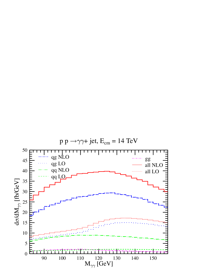
Figure 1: The invariant mass distribution of the photon pair at LHC energy. The photons and the jet are required to have transverse momentum $|p_{\rm T}|\geq 40$ GeV and lie in the central rapidity region of $|\eta|\leq 2.5$. The jet is reconstructed according to the midpoint algorithm.

In Fig. 1 we plot the invariant mass distribution of the photon pair. Here we see the continuum background on which the Higgs signal is expected to manifest itself as a narrow resonance in the intermediate-mass range. The dotted (red) line is the leading order prediction and the solid (red) one is the differential cross section at NLO accuracy. The striking feature of the plot is the rather large correction. The large corrections are partly due to the appearance of new subprocesses at NLO as can also be read off the figure. The gluon-gluon scattering subprocess begins to appear only at NLO accuracy, and therefore it is effectively leading order. It is shown with a long dashed-dotted (magenta) line: it yields a very small contribution. The bulk of the cross section comes from quark-gluon scattering both at leading order and at NLO, shown with sparsely-dotted (blue) and long-dashed (blue) lines. The quark-quark scattering receives rather large corrections because the leading order subprocess can only be a quark-antiquark annihilation process, shown with short-dashed (green) line, while at NLO, shown with short dashed-dotted (green) line, there are (anti-)quark-(anti-)quark scattering subprocesses. Thus at NLO the parton luminosity is sizeably larger. In addition, more dynamic processes are allowed, which include $t$-channel gluon exchange. These contribute to enlarge the cross section in phase space regions which are disfavoured at leading order.

A part of the large radiative corrections is accounted for by the new subprocesses; another part is due simply to the enlarged phase space, as can be seen from Fig. 2, where the differential distributions in the distance $R_{j\gamma}=\sqrt{|\eta_{j}-\eta_{\gamma}|^{2}+|\phi_{j}-\phi_{\gamma}|^{2}}$ between the jet and the photons in the $\eta$-$\phi$ plane are shown, with a selection cut at $R_{j\gamma}\geq 0.4$. We have also studied the distribution of the rapidity separation between the harder photon and the jet and we found that it is on average small. Therefore, the peak in the $R_{j\gamma_{h}}$ distribution near $\pi$ suggests that the distribution peaks where the jet and the harder photon are mostly back-to-back and central in rapidity. The harder photon is separated from the jet by at least $R_{j\gamma_{h}}\approx 2$ at leading order, while at NLO they can be as close as permitted by the selection cut. On the contrary, in going from leading order to NLO, the distribution for the photon with lower transverse momentum, the softer photon, changes in normalization but not in shape.

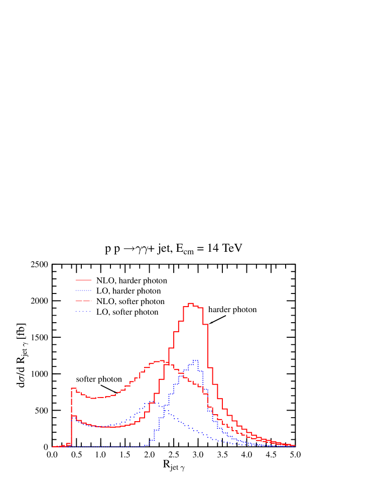
Figure 2: The distributions in the distances between the jet and the photons in the $\eta$-$\phi$ plane. The same selection cuts are used as in Fig. 1.

In the following plots, we require $R_{j\gamma}\geq 1.5$, which is also a standard selection cut in Higgs searches in the Higgs + jet channel [26, 27]. In fact, on one hand a cut on $R_{j\gamma_{s}}>1.5$ affects the leading order and the NLO evaluation in the same way because they have the same shape. Thus in that case the cut does not reduce the correction to the $m_{\scriptscriptstyle\gamma\gamma}$ distribution. On the other hand, a cut on $R_{j\gamma_{h}}>1.5$ cuts the NLO correction, but does not cut the leading order, so the correction is reduced. Nevertheless, the reduction is less then 10 %, thus cutting on $R_{j\gamma}$ at $R_{j\gamma}\geq 1.5$ reduces the NLO correction to the invariant mass distribution of the photon pair, but only marginally.

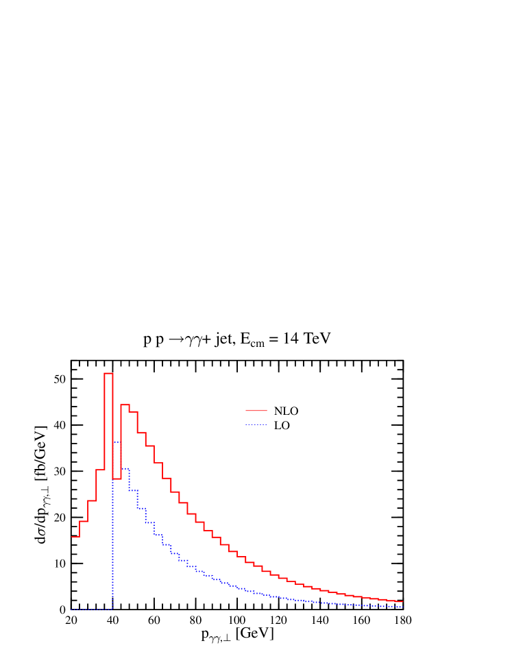
Figure 3: Transverse momentum distribution of the photon pair. The same selection cuts are used as in Fig. 1.

In Fig. 3, we plot the differential distribution of the transverse momentum of the photon pair, $p_{\gamma\gamma{\rm T}}=|{\mbox{\boldmath$p$}}_{\gamma_{1},{\rm T}}+{\mbox{\boldmath$p$}}_{\gamma_{2},{\rm T}}|$, with a cut at $p_{{\rm jet}{\rm T}}^{\rm min}=40$ GeV. At leading order the jet recoils against the photon pair and the respective jet and photon pair $p_{\rm T}$ distributions are identical. At NLO the extra parton radiation opens the part of the phase space with $p_{\gamma\gamma{\rm T}}<p_{{\rm jet}{\rm T}}^{\rm min}$. The double peak around 40 GeV is an artifact of the fixed-order computation, similar to the NLO prediction at $C=0.75$ for the $C$-parameter distribution in electron-positron annihilation. The fixed-order calculation is known to be unreliable in the vicinity of the threshold, where an all-order resummation is necessary [28], which would result in a structure, called Sudakov shoulder, that is continuous and smooth at $p_{\gamma\gamma{\rm T}}=p_{{\rm jet}{\rm T}}^{\rm min}$. Without the resummation, we must introduce a cut, $p_{\gamma\gamma,{\rm T}}\geq 40$ GeV to avoid regions in the phase space where the fixed-order prediction is not reliable. In the following plots, in addition to the default cuts, we also require $p_{\gamma\gamma,{\rm T}}\geq 40$ GeV.

The magnitude of the NLO corrections is also heavily influenced by the photon-isolation cut parameters. In Figs. 5–5 we show the effect of scanning the parameters $R_{\gamma}$ and $\epsilon$ in Eq. (25) over the values of $R_{\gamma}=0.4$, 1 and $\epsilon=0.1$, 0.5, 1. We see that the leading order predictions are independent of these parameters, but the NLO ones depend strongly on the photon isolation. Firstly, we note that the smaller $R_{\gamma}$ the larger the NLO corrections. In addition, the larger $\epsilon$ the larger the NLO correction, with the effect being larger if $R_{\gamma}$ is larger. This behaviour is in agreement with Eq. (25), according to which smaller $R_{\gamma}$ and larger $\epsilon$ imply larger amounts of soft-parton energy that is allowed inside the cone.

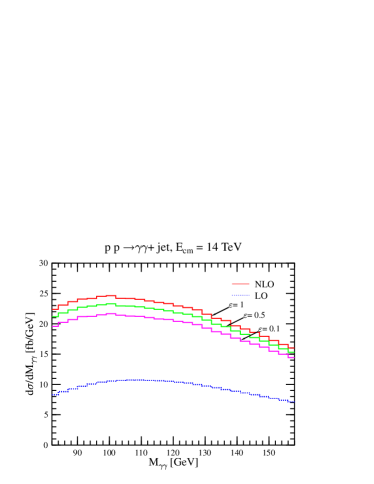
Figure 4: Dependence of the invariant mass distribution of the photon pair on the photon isolation parameter $\epsilon$ for $R_{\gamma}=0.4$. In addition to the selection cuts used in Fig. 1, we also require $R_{j\gamma}\geq 1.5$ and $p_{\gamma\gamma,{\rm T}}\geq 40$ GeV.

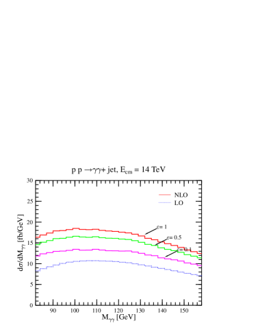
Figure 5: Dependence of the invariant mass distribution of the photon pair on the photon isolation parameter $\epsilon$ for $R_{\gamma}=1$. The same selection cuts are used as in Fig. 4.

Another remarkable feature of Figs. 5–5 is that with the applied cuts, the two-photon plus jet background for the search of a Higgs boson with mass in the 120–140 GeV range is rather flat, therefore, well measurable from the sidebands around the hypothetical Higgs signal. This feature is very different from the shape of the background to the inclusive $pp\to H\to\gamma\gamma$ channel, which is steeply falling.

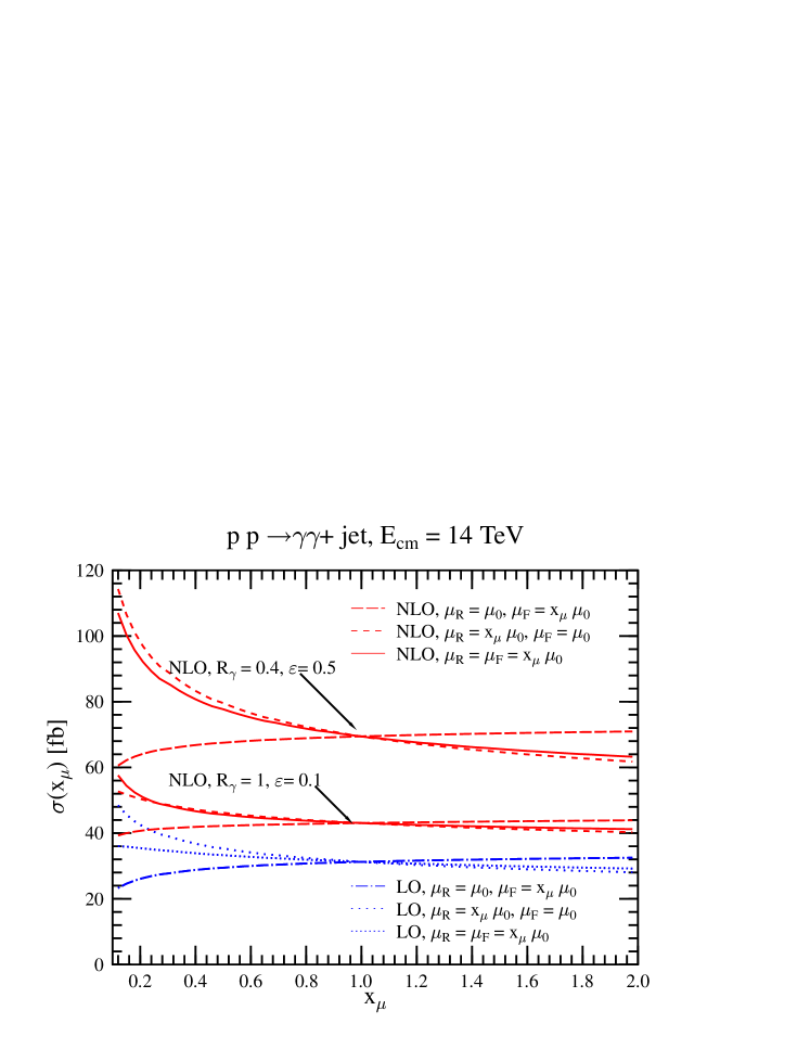
Figure 6: Dependence on the renormalization and factorization scales of the cross section in a bin of 118.5 GeV $\leq m_{\scriptscriptstyle\gamma\gamma}\leq$ 121.5 GeV at leading-order and at NLO accuracy. The same selection cuts are used as in Fig. 4.

In order to assess the stability of the predictions against scale variations, we show the cross section in a 3 GeV bin around $m_{\scriptscriptstyle\gamma\gamma}=120$ GeV, that is the background for a hypothetical Higgs signal for a Higgs particle of mass 120 GeV. Fig. 6 shows the cross section for two sets of photon-isolation parameters. We show the scale variations for varying the renormalization and factorization scales separately, keeping the other scale fixed, as well as varying them simultaneously. The lower three curves represent the leading order predictions. At leading order the dependence on the renormalization and factorization scales is rather small, especially when the two scales are set equal (densely dotted line). Observing the predictions we conclude that the scale dependence at leading order does not represent the uncertainty of the predictions due to the unknown higher orders. The inclusion of the radiative corrections results mainly in the substantial increase of the cross section. For our default isolation ($R_{\gamma}=0.4$ and $\epsilon=0.5$) the NLO corrections at $x_{\mu}=1$ are about 120 % of the leading order prediction. In addition, the scale dependence is not reduced by the inclusion of the radiative corrections. If we require more stringent photon isolation cuts, then we find smaller corrections and a more stable prediction. For instance, in Fig. 6 we also show the scale dependence of the cross section obtained with $R_{\gamma}=1$ and $\epsilon=0.1$. We find that the cross section at NLO is about 40 % larger than the leading order prediction, and in this case the scale dependence at NLO is reduced as compared to the one at leading order accuracy.

4 Conclusions

In this paper we computed the QCD radiative corrections to the $pp\to\gamma\gamma+{\rm jet}$ process that constitutes part of the irreducible background to the $pp\to H+{\rm jet}\to\gamma\gamma+{\rm jet}$ discovery channel of an intermediate-mass Higgs boson at the LHC. We used a smooth photon isolation that is infrared safe to all orders in perturbation theory and independent of the photon fragmentation into hadrons. The predictions were made with a partonic Monte Carlo program that can be utilized for a detailed study of the signal significance for the intermediate-mass Higgs boson discovery in the Higgs + jet production channel at the LHC. We found large radiative corrections, however they are rather sensitive to the selection cuts and photon isolation parameters. Choosing a mild photon isolation, i.e. a small isolation cone radius $R_{\gamma}=0.4$ with relatively large hadronic activity allowed in the cone results in more than 100 % correction with as large residual scale dependence at NLO as at leading order. Making the photon isolation more stringent, for instance increasing the cone radius to $R_{\gamma}=1$ and decreasing the hadronic activity in the cone reduces both the magnitude of the radiative corrections as well as the dependence on the renormalization and factorization scales. This result shows that a constant $K^{\rm NLO}=1.6$ factor, as mentioned in the Introduction, is certainly not appropriate for taking into account the radiative corrections to the irreducible background of the $pp\to H+{\rm jet}\to\gamma\gamma+{\rm jet}$ discovery channel at the LHC.

References

- [1] M. N. Dubinin, V. A. Ilyin and V. I. Savrin, Search for Higgs boson at LHC in the reaction p p gamma gamma + jet at a low luminosity, [hep-ph/9712335].
- [2] S. Abdullin, M. Dubinin, V. Ilyin, D. Kovalenko, V. Savrin and N. Stepanov, Higgs boson discovery potential of LHC in the channel p p gamma gamma + jet, Phys. Lett. B 431 (1998) 410 [hep-ph/9805341].
- [3] R. K. Ellis, I. Hinchliffe, M. Soldate and J. J. van der Bij, Higgs decay to : a possible signature of intermediate mass Higgs bosons at the SSC, Nucl. Phys. B 297 (1988) 221.
- [4] E. E. Boos, M. N. Dubinin, V. A. Ilin, A. E. Pukhov and V. I. Savrin, CompHEP: Specialized package for automatic calculations of elementary particle decays and collisions, [hep-ph//9503280].
- [5] D. de Florian, M. Grazzini and Z. Kunszt, Higgs production with large transverse momentum in hadronic collisions at next-to-leading order, Phys. Rev. Lett. 82 (1999) 5209 [hep-ph/9902483].
- [6] D. de Florian and Z. Kunszt, Two photons plus jet at LHC: The NNLO contribution from the g g initiated process, Phys. Lett. B 460 (1999) 184 [hep-ph/9905283].
- [7] C. Balazs, P. Nadolsky, C. Schmidt and C. P. Yuan, Diphoton background to Higgs boson production at the LHC with soft gluon effects, Phys. Lett. B 489 (2000) 157 [hep-ph/9905551].
- [8] S. J. Parke and T. R. Taylor, An Amplitude For N Gluon Scattering, Phys. Rev. Lett. 56 (1986) 2459.
- [9] V. Barger, T. Han, J. Ohnemus and D. Zeppenfeld, Pair Production Of W+-, Gamma And Z In Association With Jets, Phys. Rev. D 41 (1990) 2782.
- [10] V. Del Duca, W. B. Kilgore and F. Maltoni, Multiphoton amplitudes for next-to-leading order QCD, Nucl. Phys. B 574 (2000) 851 [hep-ph/9910253]
- [11] M. L. Mangano and S. J. Parke, Multiparton amplitudes in gauge theories, Phys. Rev. C 200 (1991) 301.
- [12] Z. Bern, L. Dixon and D. A. Kosower, One loop corrections to two quark three gluon amplitudes, Nucl. Phys. B 437 (1995) 259 [hep-ph/9409393].
- [13] A. Signer, One loop corrections to five parton amplitudes with external photons, Phys. Lett. B 357 (1995) 204 [hep-ph/9507442].
- [14] S. Catani and M. H. Seymour, A general algorithm for calculating jet cross sections in NLO QCD, Nucl. Phys. B 485, 291 (1997) [Erratum-ibid. B 510, 503 (1997)] [hep-ph/9605323].
- [15] Z. Nagy and Z. Trocsanyi, Next-to-leading order calculation of four-jet observables in electron positron annihilation, Phys. Rev. D 59, 014020 (1999) [Erratum-ibid. D 62, 099902 (2000)] [hep-ph/9806317].
- [16] Z. Nagy, Three-jet cross sections in hadron hadron collisions at next-to-leading order, Phys. Rev. Lett. 88 (2002) 122003 [hep-ph/0110315]
- [17] R. Gastmans and T.T. Wu, The ubiquitous photon: Helicity Method for QED and QCD, Clarendon Press, 1990.
- [18] W. Siegel, Supersymmetric Dimensional Regularization Via Dimensional Reduction, Phys. Lett. B 84 (1979) 193.
- [19] D. M. Capper, D. R. Jones and P. van Nieuwenhuizen, Regularization By Dimensional Reduction Of Supersymmetric And Nonsupersymmetric Gauge Theories, Nucl. Phys. B 167 (1980) 479.
- [20] Z. Bern and D. A. Kosower, The Computation of loop amplitudes in gauge theories, Nucl. Phys. B 379 (1992) 451.
- [21] A. D. Martin, R. G. Roberts, W. J. Stirling and R. S. Thorne, MRST2001: Partons and alpha(s) from precise deep inelastic scattering and Tevatron jet data, Eur. Phys. J. C 23, 73 (2002) [hep-ph/0110215].
- [22] J. Pumplin, D. R. Stump, J. Huston, H. L. Lai, P. Nadolsky and W. K. Tung, New generation of parton distributions with uncertainties from global QCD analysis, JHEP 0207, 012 (2002) [hep-ph/0201195].
- [23] G. C. Blazey et al., “Run II jet physics, [hep-ex/0005012].
- [24] S. Catani, M. Fontannaz, J. P. Guillet and E. Pilon, Cross section of isolated prompt photons in hadron hadron collisions, JHEP 0205, 028 (2002) [hep-ph/0204023].
- [25] S. Frixione, Isolated photons in perturbative QCD, Phys. Lett. B 429 (1998) 369 [hep-ph/9801442].
- [26] CMS Collaboration, Technical Proposal, report CERN/LHCC 94-38 (1994)
- [27] ATLAS Collaboration, Detector and Physics Performance Technical Design Report, Vol. II, report CERN/LHCC 99-15 (1999).
- [28] S. Catani and B. R. Webber, Infrared safe but infinite: Soft-gluon divergences inside the physical region, JHEP 9710, 005 (1997) [hep-ph/9710333].