The chirally-odd twist-3 distribution function $e^{a}(x)$
in the chiral quark-soliton model

Abstract

The chirally-odd twist-3 nucleon distribution $e^{a}(x)$ is studied in the large-$N_{c}$ limit in the framework of the chiral quark-soliton model at a low normalization point of about $0.6\,{\rm GeV}$. The remarkable result is that in the model $e^{a}(x)$ contains a $\delta$-function-type singularity at $x=0$. The regular part of $e^{a}(x)$ is found to be sizeable at the low scale of the model and in qualitative agreement with bag model calculations.

I Introduction

In deeply inelastic scattering (DIS) processes the nucleon structure up to twist-3 is described by six parton distribution functions, the twist-2 $f_{1}^{a}(x)$, $g_{1}^{a}(x)$, $h_{1}^{a}(x)$ and the twist-3 $e^{a}(x)$, $g_{T}^{a}(x)$, $h_{L}^{a}(x)$. Among these functions the least considered one is probably the twist-3 chirally odd distribution function $e^{a}(x)$ Jaffe:1991kp ; Jaffe:1991ra , which contrasts the fact that it is related to several interesting phenomena. E.g., a known Balitsky:1996uh ; Belitsky:1997zw ; Koike:1997bs ; Belitsky:1997ay ; Kodaira:1998jn but rarely emphasized Efremov:2002qh fact is that $e^{a}(x)$ contains a $\delta$-function-type singularity at $x=0$, as follows from the QCD equations of motion. The existence of a $\delta(x)$-contribution also was concluded from perturbative calculations Burkardt:2001iy . The first Mellin moment of $e^{a}(x)$ is due to the $\delta(x)$-contribution only. Another interesting phenomenon is connected to the first Mellin moment of the flavour-singlet $(e^{u}+e^{d})(x)$ which is proportional to the pion-nucleon sigma-term $\sigma_{\mbox{\tiny$\pi$N}}$. The latter gives rise to the so-called “sigma-term puzzle”. The large value extracted from pion-nucleon scattering data, $\sigma_{\mbox{\tiny$\pi$N}}\approx(50-70)\,{\rm MeV}$ Koch:pu ; Pavan:2001wz , implies that about $20\%$ of the nucleon mass $M_{\mbox{\tiny N}}$ is due to the strange quark – an unexpectedly large number from the point of view of the OZI-rule.

The reason why $e^{a}(x)$ has received only little attention so far is related to its chiral odd nature, which means that $e^{a}(x)$ can enter an observable only in connection with another chirally odd distribution or fragmentation function, and therefore is difficult to access in experiments. Only recently it was shown that $e^{a}(x)$ can be accessed by means of the “Collins effect” collins , i.e.  the left-right asymmetry in the fragmentation of a transversely polarized quark into a pion. This effect is described by the chirally and T-odd fragmentation function $H_{1}^{\perp a}(z)$, which is “twist-2” in the sense that its contribution to an observable is not power suppressed collins ; muldt . First experimental indications to $H_{1}^{\perp}$ were reported in Efremov:1998vd . Assuming factorization it was shown that the Collins effect gives rise to a specific azimuthal (with respect to the axis defined by the exchanged hard virtual photon) distribution of pions produced in DIS of longitudinally polarized electrons off an unpolarized proton target. The observable single (beam) spin asymmetry is proportional to $\sum_{a}e_{a}^{2}\,e^{a}(x)\,H_{1}^{\perp a}(z)$ Mulders:1996dh ($e_{a}=\pm\frac{2}{3},\pm\frac{1}{3}$ are the quark electric charges). The process was studied in the HERMES experiment and the effect found consistent with zero within error bars hermes . However, in the CLAS experiment, in a different kinematics, a sizeable asymmetry was observed Avakian-talk ; Avakian:2003pk . If the interpretation applies, that the CLAS data Avakian-talk ; Avakian:2003pk are due to the Collins effect, then $e^{a}(x)$ is definitely not small. Using estimates of $H_{1}^{\perp}(z)$ from HERMES data Efremov:2001cz it was shown in Efremov:2002sd , that $e^{a}(x)$ could be about half the magnitude of the unpolarized twist-2 distribution $f_{1}^{a}(x)$ at $Q^{2}\sim 1.5\,{\rm GeV}^{2}$ in the region $0.15\leq x\leq 0.4$ covered in the CLAS experiment.

The indication that $e^{a}(x)$ could be large in the valence-$x$ region is not surprising, if one considers results from the bag model Jaffe:1991ra ; Signal:1997ct , the only model where $e^{a}(x)$ has been studied so far. In this note $e^{a}(x)$ will be studied in the chiral quark-soliton model ($\chi$QSM). A subtle question is whether models with no gluon degrees of freedom (bag model, $\chi$QSM) can describe twist-3 distribution functions. The answer given in Jaffe:1991kp ; Jaffe:1991ra is yes, because $e^{a}(x)$, $g_{T}^{a}(x)$ and $h_{L}^{a}(x)$ are special cases of more general quark-gluon-quark correlation functions; special inasmuch they do not contain explicit gluon fields. However, implicitly gluons do contribute and it is important and instructive to carefully interpret the results. E.g., in the bag model $e^{a}(x)$ is due to the bag boundary Jaffe:1991ra . This can be understood considering that the bag boundary (in a most intuitive way) models confinement, and thus “mimics” gluons.

The $\chi$QSM was derived from the instanton model of the QCD vacuum. An important small parameter in this derivation is the “instanton packing fraction” which characterizes the diluteness of the instanton medium Diakonov:1985eg ; Diakonov:1983hh . Gluon degrees of freedom appear only at next-to-leading order of this parameter Diakonov:1995qy . In leading order of the instanton packing fraction the $\chi$QSM quark degrees of freedom can be identified with the QCD quark degrees of freedom. This allows to consistently describe twist-2 quark and antiquark distribution functions $f_{1}^{a}(x)$, $g_{1}^{a}(x)$ and $h_{1}^{a}(x)$ at a low scale around $600\,{\rm MeV}$ Diakonov:1996sr . The numerical results Diakonov:1996sr ; Diakonov:1997vc ; Weiss:1997rt ; Pobylitsa:1996rs ; Goeke:2000wv agree within $(10-30)\%$ with parameterizations for the “known” distribution functions performed at low scales GRV+GRSV .

The twist-3 distribution functions $g_{T}^{a}(x)$ and $h_{L}^{a}(x)$ were studied in the instanton vacuum model in Refs. Balla:1997hf ; Dressler:2000hc . The remarkable conclusion was that the pure twist-3 interaction dependent parts $\widetilde{g}_{T}^{a}(x)$ and $\widetilde{h}_{L}^{a}(x)$ in the Wandzura-Wilczek(-like) decompositions of $g_{T}^{a}(x)$ and $h_{L}^{a}(x)$ are strongly suppressed by powers of the instanton packing fraction. As $g_{T}^{a}(x)$ and $h_{L}^{a}(x)$ do not contain explicit gluon fields it is possible to evaluate $g_{T}^{a}(x)$ and $h_{L}^{a}(x)$ directly in the $\chi$QSM. This was done in Refs. Wakamatsu:2000ex ; Wakamatsu:2001fd , and it was observed that the pure twist-3 parts $\widetilde{g}_{T}^{a}(x)$ and $\widetilde{h}_{L}^{a}(x)$ are indeed small. Thus in these cases the $\chi$QSM respects the results found directly in the instanton vacuum model – i.e.  the theory from which it was derived. This experience encourages to also tackle the study of $e^{a}(x)$ in the $\chi$QSM. However, one has to keep in mind that the results and their interpretation presented here should also be reexamined in the instanton vacuum model. This is out of the scope of this note and left for future studies.

The $\chi$QSM describes the nucleon as a chiral soliton of the pion field in the limit of a large number of colours $N_{c}$. This note focuses on the flavour singlet distributions $(e^{u}+e^{d})(x)$ and $(e^{\bar{u}}+e^{\bar{d}})(x)$ – the leading flavour combinations in the large-$N_{c}$ limit. The consistency of the approach is checked, by demonstrating that the model expressions for $(e^{u}+e^{d})(x)$ satisfy QCD sum rules. It is shown that the model expressions are (quadratically and logarithmically) UV-divergent, and a consistent regularization is defined. Remarkably, it is found that the $\chi$QSM-expression for $(e^{u}+e^{d})(x)$ contains a $\delta(x)$-contribution. The UV-behaviour and the $\delta(x)$-contribution make an exact numerical evaluation of $(e^{u}+e^{d})(x)$ and $(e^{\bar{u}}+e^{\bar{d}})(x)$ particularly involved. Therefore $(e^{u}+e^{d})(x)$ is evaluated using an approximation, the “interpolation formula” of Ref. Diakonov:1996sr .

This note is organized as follows. In Sec. II the twist-3 distribution function $e^{a}(x)$ and some of its properties are discussed. Sec. III contains a brief introduction into the $\chi$QSM. In Sec. IV the flavour-singlet distribution $(e^{u}+e^{d})(x)$ is discussed and evaluated in the model using the interpolation formula. In Sec. V $e^{a}(x)$ is discussed in the non-relativistic limit. Sec. VI contains a summary and conclusions.

II The distribution function $e^{a}(x)$

The chirally odd twist-3 distribution functions $e^{q}(x)$ for quarks of flavour $q$ and $e^{\bar{q}}(x)$ for antiquarks of flavour $\bar{q}$ are defined as Jaffe:1991kp ; Jaffe:1991ra

$$e^{q}(x)=\frac{1}{2M_{\mbox{\tiny N}}}\int\!\frac{{\rm d}\lambda}{2\pi}\,e^{i\lambda x}\,\langle N|\,\bar{\psi}_{q}(0)\,[0,\lambda n]\,\psi_{q}(\lambda n)\,|N\rangle\;,\;\;\;e^{\bar{q}}(x)=e^{q}(-x)\;,$$ (1)

where $[0,\lambda n]$ denotes the gauge-link. The scale dependence is not indicated for brevity. The light-like vectors $n^{\alpha}$ in Eq. (1) and $p^{\alpha}$ are defined such that $n^{\alpha}p_{\alpha}=1$ and the nucleon momentum is given by $P^{\alpha}_{\mbox{\tiny N}}=n^{\alpha}+p^{\alpha}M_{\mbox{\tiny N}}^{2}/2$. The matrix element in Eq. (1) is averaged over nucleon spin, i.e. $\langle N|\dots|N\rangle\equiv\frac{1}{2}\sum_{S_{3}}\langle N,S_{3}|\dots|N,S_{3}\rangle$.

The renormalization scale evolution of $e^{a}(x)$ was studied in Refs. Balitsky:1996uh ; Belitsky:1997zw ; Koike:1997bs , see also Refs. Belitsky:1997ay ; Kodaira:1998jn for reviews. It evolves according to an evolution pattern typical for twist-3 quantities. It is not sufficient to know the $n^{\rm th}$ Mellin-moment ${\cal M}_{n}[e^{a}](Q_{0}^{2})=\int{\rm d}x\,x^{n-1}e^{a}(x,Q_{0}^{2})$ at an initial scale $Q_{0}^{2}$, in order to compute ${\cal M}_{n}[e^{a}](Q^{2})$ for $Q^{2}>Q_{0}^{2}$. Instead, the knowledge of all moments ${\cal M}_{k}[e^{a}](Q^{2}_{0})$ with $k\leq n$ is required. In the limit of a large number of colours $N_{c}$ the evolution of $e^{a}(x)$ simplifies to a DGLAP-type evolution – as it does for the other two proton twist-3 distributions $h_{L}^{a}(x)$ and (the flavour non-singlet) $g_{T}^{a}(x)$.

The QCD-equations of motion allow to decompose $e^{q}(x)$ in a gauge-invariant way as Balitsky:1996uh ; Belitsky:1997zw ; Koike:1997bs , see also Belitsky:1997ay ; Kodaira:1998jn and Efremov:2002qh ,

$$e^{q}(x)=\delta(x)\,\frac{1}{2M_{\mbox{\tiny N}}}\,\langle N|\bar{\psi}_{q}(0)\psi_{q}(0)|N\rangle+e^{q}_{tw3}(x)+\frac{m_{q}}{M_{\mbox{\tiny N}}}\;\frac{f_{1}^{q}(x)}{x}\;\delta_{n>1}\;\;.$$ (2)

The $\delta(x)$-contribution has no partonic interpretation. Some authors cancel it out by multiplying $e^{q}(x)$ by $x$, while others prefer to consider from the beginning an alternative definition of $e^{q}(x)$ with an explicit factor of $x$ on the RHS of Eq. (1). The existence of a $\delta(x)$-contribution also was concluded in Ref. Burkardt:2001iy , where $e^{q}(x)$ was constructed explicitly for a one-loop dressed massive quark. The contribution $e^{q}_{tw3}(x)$ in Eq. (2) is a quark-gluon-quark correlation function, i.e. the actual “pure” twist-3 (“interaction dependent”) contribution to $e^{a}(x)$, and has a partonic interpretation as an interference between scattering from a coherent quark-gluon pair and from a single quark Jaffe:1991kp ; Jaffe:1991ra . Its first two moments vanish. The third (“mass”-) term in Eq. (2) vanishes in the chiral limit. The “Kronecker symbol” $\delta_{n>1}$ accompanying it has the following meaning. The first moment of the mass-term vanishes. For $x\neq 0$ the expression in Eq. (2) is, however, correct and can be used literally to take higher moments $n>1$.

The first and the second moment of $e^{q}(x)$ satisfy the sum rules Jaffe:1991kp ; Jaffe:1991ra

$$\int_{-1}^{1}{\rm d}x\;e^{q}(x) = \frac{1}{2M_{\mbox{\tiny N}}}\langle N|\,\bar{\psi}_{q}(0)\psi_{q}(0)\,|N\rangle\;,$$ (3)

$$\int_{-1}^{1}{\rm d}x\;x\,e^{q}(x) = \frac{m_{q}}{M_{\mbox{\tiny N}}}\;N_{q}\;.$$ (4)

In Eq. (4) $N_{q}$ denotes the number of the respective valence quarks (for proton $N_{u}=2$ and $N_{d}=1$). The sum rules (3, 4) follow immediately from the decomposition in Eq. (2) and the above mentioned properties of $e^{q}_{tw3}(x)$ and the mass-term. In particular, the sum rule (3) is saturated by the $\delta(x)$-contribution in Eq. (2).

The flavour singlet distribution function $(e^{u}+e^{d})(x)$ is related to the scalar isoscalar nucleon form-factor $\sigma(t)$ defined as

$$\sigma(t)\;\bar{u}_{N}({\bf P^{\prime}})u_{N}({\bf P})=m\;\langle N({\bf P^{\prime}})|\,\biggl{(}\bar{\psi}_{u}(0)\psi_{u}(0)+\bar{\psi}_{d}(0)\psi_{d}(0)\biggr{)}\,|N({\bf P})\rangle\;\;,\;\;\;t=(P^{\prime}-P)^{2}\;,$$ (5)

where $u_{N}$ denotes the nucleon spinor (normalized as $\bar{u}_{N}u_{N}=2M_{\mbox{\tiny N}}$) and $m=\frac{1}{2}\,(m_{u}+m_{d})$. In (5) a term proportional to $(m_{u}-m_{d})(\bar{\psi}_{u}\psi_{u}-\bar{\psi}_{d}\psi_{d})$ is neglected. At the point $t=0$ the form-factor $\sigma(t)$ is referred to as the pion-nucleon sigma-term $\sigma_{\mbox{\tiny$\pi$N}}$ and related to $(e^{u}+e^{d})(x)$ by means of the sum rule (3) as

$$\sigma_{\mbox{\tiny$\pi$N}}\equiv\sigma(0)=m\int_{-1}^{1}{\rm d}x\;(e^{u}+e^{d})(x)\;\;.$$ (6)

The form factor $\sigma(t)$ describes the elastic scattering off the nucleon due to the exchange of a spin-zero particle and is not measured yet. However, low-energy theorems allow to deduce its value at the Cheng-Dashen point $t=2m_{\pi}^{2}$ from pion-nucleon scattering data. One finds

$$\sigma(2m_{\pi}^{2})=\cases{(64\pm 8)\,{\rm MeV}&Ref.~{}\cite[cite]{\@@bibref{Authors Phrase1YearPhrase2}{Koch:pu}{\@@citephrase{(}}{\@@citephrase{)}}}\cr(79\pm 7)\,{\rm MeV}&Ref.~{}\cite[cite]{\@@bibref{Authors Phrase1YearPhrase2}{Pavan:2001wz}{\@@citephrase{(}}{\@@citephrase{)}}}.}$$ (7)

The difference $\sigma(2m_{\pi}^{2})-\sigma(0)$ was obtained from a dispersion relation analysis Gasser:1990ce and chiral perturbation theory calculations Becher:1999he with the consistent result of $14\;{\rm MeV}$. This yields

$$\sigma_{\mbox{\tiny$\pi$N}}\approx(50-70)\;{\rm MeV}\;.$$ (8)

With $m\approx(5-8)\,{\rm MeV}$ one obtains a large number for the first moment of $(e^{u}+e^{d})(x)$

$$\int_{-1}^{1}{\rm d}x\;(e^{u}+e^{d})(x)\approx 10\;.$$ (9)

One should keep in mind, however, that the large number in Eq. (9) is not due to a large “valence” structure in $(e^{u}+e^{d})(x)$, but solely due to the $\delta(x)$-contribution.

III The chiral quark soliton model ($\chi$QSM)

The $\chi$QSM is based on the effective chiral relativistic quantum field theory given by the partition function Diakonov:1985eg ; Diakonov:1987ty ; Diakonov:tw

$$Z_{\rm eff}=\int\!\!{\cal D}\psi\,{\cal D}\bar{\psi}\,{\cal D}U\;\exp\Biggl{(}i\int\!\!{\rm d}^{4}x\;\bar{\psi}\,(i{\not\!\partial\,}-M\,U^{\gamma_{5}}-m)\psi\Biggr{)}\;\;,$$ (10)

$$U=\exp(i\tau^{a}\pi^{a})\;\;,\;\;\;U^{\gamma_{5}}=\frac{1}{2}(U+U^{\dagger})+\frac{1}{2}(U-U^{\dagger})\gamma_{5}\;.$$ (11)

In Eq. (10) $M$ is the (generally momentum dependent) dynamical quark mass, which is due to spontaneous breakdown of chiral symmetry. $U$ denotes the $SU(2)$ chiral pion field. The current quark mass $m$ in Eq. (10) explicitly breaks the chiral symmetry and can be set to zero in many applications. For certain quantities, however, it is convenient or even necessary to consider finite $m$. The effective theory (10) contains the Wess-Zumino term and the four-derivative Gasser-Leutwyler terms with correct coefficients. It has been derived from the instanton model of the QCD vacuum Diakonov:1983hh ; Diakonov:1987ty , and is valid at low energies below a scale set by the inverse of the average instanton size

$$\rho_{\rm av}^{-1}\approx 600\,{\rm MeV}\;.$$ (12)

In practical calculations it is convenient to take the momentum dependent quark mass constant, i.e. $M(p)\to M(0)=350\,{\rm MeV}$. In this case $\rho_{\rm av}^{-1}$ is to be understood as the cutoff, at which quark momenta have to be cut off within some appropriate regularization scheme. It is important to remark that $(M\rho_{\rm av})^{2}$ is proportional to the parametrically small instanton packing fraction

$$(M\rho_{\rm av})^{2}\propto\biggl{(}\frac{\rho_{\rm av}}{R_{\rm av}}\biggr{)}^{\!4}\ll 1\;,$$ (13)

with $R_{\rm av}$ denoting the average distance between instantons. The smallness of this quantity has been used in the derivation of the effective theory (10) from the instanton vacuum model Diakonov:1983hh ; Diakonov:1987ty .

The $\chi$QSM is an application of the effective theory (10) to the description of baryons Diakonov:1987ty . The large-$N_{c}$ limit allows to solve the path integral over pion field configurations in Eq. (10) in the saddle-point approximation. In the leading order of the large-$N_{c}$ limit the pion field is static, and one can determine the spectrum of the one-particle Hamiltonian of the effective theory (10)

$$\hat{H}|n\rangle=E_{n}|n\rangle\;,\;\;\hat{H}=-i\gamma^{0}\gamma^{k}\partial_{k}+\gamma^{0}MU^{\gamma_{5}}+\gamma^{0}m\;.$$ (14)

The spectrum consists of an upper and a lower Dirac continuum, distorted by the pion field as compared to continua of the free Dirac-Hamiltonian

$$\hat{H}_{0}|n_{0}\rangle=E_{n_{0}}|n_{0}\rangle\;\;,\;\;\;\;\hat{H}_{0}=-i\gamma^{0}\gamma^{k}\partial_{k}+\gamma^{0}M+\gamma^{0}m\;,$$ (15)

and of a discrete bound state level of energy $E_{\rm lev}$, if the pion field is strong enough. By occupying the discrete level and the states of the lower continuum each by $N_{c}$ quarks in an anti-symmetric colour state, one obtains a state with unity baryon number. The soliton energy $E_{\rm sol}$ is a functional of the pion field

$$E_{\rm sol}[U]=N_{c}\biggl{(}E_{\rm lev}+\sum\limits_{E_{n}<0}(E_{n}-E_{n_{0}})\biggr{)}\biggr{|}_{\rm reg}\;.$$ (16)

$E_{\rm sol}[U]$ is logarithmically divergent and has to be regularized appropriately, as indicated in (16). Minimization of $E_{\rm sol}[U]$ determines the self-consistent soliton field $U_{c}$. This procedure is performed for symmetry reasons in the so-called hedgehog ansatz

$$\pi^{a}({\bf x})=e_{r}^{a}\;P(r)\;,\;\;U({\bf x})=\cos P(r)+i\tau^{a}e_{r}^{a}\sin P(r)\;,$$ (17)

with $r=|{\bf x}|$ and $e_{r}^{a}=x^{a}/r$, in which the variational problem reduces to the determination of the self-consistent soliton profile $P_{c}(r)$. The nucleon mass $M_{\mbox{\tiny N}}$ is given by $E_{\rm sol}[U_{c}]$. The momentum and the spin and isospin quantum numbers of the baryon are described by considering zero modes of the soliton. Corrections in the $1/N_{c}$-expansion can be included by considering time dependent pion field fluctuations around the solitonic solution. A good and for many purposes sufficient approximation to the self-consistent profile $P_{c}(r)$ is given by the analytical “arctan-profile”

$$P(r,m_{\pi})=-2\,{\rm arctan}\biggl{(}\frac{R^{2}_{sol}}{r^{2}}(1+m_{\pi}r)e^{-m_{\pi}r}\biggr{)}\;,\;\;R_{sol}=M^{-1}\;,$$ (18)

where $R_{sol}$ is the soliton size. In the chiral limit $m\to 0$ in (10) the self-consistent profile $P_{c}(r)\propto 1/r^{2}$ for $r\to\infty$, and then $m_{\pi}=0$ in (18). If $m\neq 0$ in (10) the self-consistent profile exhibits a Yukawa-tail $P_{c}(r)\propto e^{-m_{\pi}r}/r$ for $r\to\infty$ and $m_{\pi}$ is the physical pion mass connected to the current quark mass $m$ in (10) by the Gell-Man–Oakes–Renner relation (see below Eq. (62)). The analytical profile (18) simulates this and the Gell-Mann–Oakes–Renner relation holds approximately.

The $\chi$QSM allows to evaluate in a parameter-free way nucleon matrix elements of QCD quark bilinear operators as (schematically)

$$\langle N|\bar{\psi}(z_{1})\Gamma\psi(z_{2})|N\rangle=c_{\mbox{\tiny$\Gamma$}}2M_{\mbox{\tiny N}}N_{c}\sum\limits_{n\,\rm occ}\int\!\!{\rm d}^{3}{\bf X}\>\bar{\Phi}_{n}({\bf z}_{1}-{\bf X})\Gamma\Phi_{n}({\bf z}_{2}-{\bf X})\,e^{iE_{n}(z^{0}_{1}-z^{0}_{2})}+\dots\;\,$$ (19)

$$=-c_{\mbox{\tiny$\Gamma$}}2M_{\mbox{\tiny N}}N_{c}\sum\limits_{n\,\rm non}\int\!\!{\rm d}^{3}{\bf X}\>\bar{\Phi}_{n}({\bf z}_{1}-{\bf X})\Gamma\Phi_{n}({\bf z}_{2}-{\bf X})\,e^{iE_{n}(z^{0}_{1}-z^{0}_{2})}+\dots\;.$$ (20)

In Eqs. (19, 20) $\Gamma$ is some Dirac- and flavour-matrix, $c_{\mbox{\tiny$\Gamma$}}$ a constant depending on $\Gamma$ and the spin and flavour quantum numbers of the nucleon state $|N\rangle=|S_{3},T_{3}\rangle$, and $\Phi_{n}({\bf x})=\langle{\bf x}|n\rangle$ are the coordinate space wave-functions of the single quark states $|n\rangle$ in (14). The sum in Eq. (19) goes over occupied levels $n$ (i.e. $n$ with $E_{n}\leq E_{\rm lev}$), and vacuum subtraction is implied for $E_{n}<E_{\rm lev}$ analogue to Eq. (16). The sum in Eq. (20) goes over non-occupied levels $n$ (i.e. $n$ with $E_{n}>E_{\rm lev}$), and vacuum subtraction is implied for all $E_{n}>E_{\rm lev}$. The dots in Eqs. (19, 20) denote terms subleading in the $1/N_{c}$-expansion, which will not be needed in this work. Depending on the Dirac- and flavour-structure the expressions (19, 20) can possibly be UV-divergent and need to be regularized. If in QCD the quantity on the LHS of Eq. (19) is normalization scale dependent, the model results refer to a scale roughly set by $\rho_{\rm av}^{-1}$ in Eq. (12).

In the way sketched in (19, 20) static nucleon properties (form-factors, axial properties, etc., see Christov:1995vm for a review), twist-2 Diakonov:1996sr ; Diakonov:1997vc ; Weiss:1997rt ; Pobylitsa:1996rs ; Goeke:2000wv and twist-3 Wakamatsu:2000ex ; Wakamatsu:2001fd quark and antiquark distribution functions, and off-forward distribution functions Petrov:1998kf have been studied in the $\chi$QSM. As far as those quantities are known, the model results agree within $(10-30)\%$ with experiment or phenomenology. It is important to note the theoretical consistency of the approach, in particular the quark and antiquark distribution functions in the model satisfy all general QCD requirements (sum rules, positivity, inequalities, etc.).

IV $e^{a}(x)$ in the $\chi$QSM

IV.1 Expressions and consistency

Model expressions.

The model expressions for the flavour combinations $(e^{u}\pm e^{d})(x)$ “follow” from the expressions for the unpolarized twist-2 distributions $(f_{1}^{u}\pm f_{1}^{d})(x)$ derived in Ref. Diakonov:1996sr by “replacing” the relevant Dirac-structure $n^{\alpha}\gamma_{\alpha}$ in the definition of $f_{1}^{a}(x)$ by $1/M_{\mbox{\tiny N}}$. This can be checked by an explicit calculation which closely follows the derivation given in Diakonov:1996sr and can therefore be skipped here. This “analogy” between $e^{a}(x)$ and $f_{1}^{a}(x)$ is due to the fact that both are “spin average” distributions, and the relevant Dirac- and flavour-structures exhibit the same properties under the hedgehog symmetry transformations. As a consequence, the flavour combinations $(e^{u}\pm e^{d})(x)$ have the same large-$N_{c}$ behaviour as $(f_{1}^{u}\pm f_{1}^{d})(x)$ Diakonov:1996sr , namely

$$(e^{u}+e^{d})(x) = N_{c}^{2}\>d(N_{c}x)$$

$$(e^{u}-e^{d})(x) = N_{c}\,\>d(N_{c}x)\;,$$ (21)

where the functions $d(y)$ are stable in the limit $N_{c}\to\infty$ for fixed arguments $y=N_{c}x$, and different for the different flavour combinations. Though derived in the $\chi$QSM, the relations in (IV.1) are of general character, considering that the $\chi$QSM is a particular realization of the large-$N_{c}$ picture of the nucleon Witten:1979kh . The relations (IV.1) are already the end of the story of “analogies” between $e^{a}(x)$ and $f_{1}^{a}(x)$ in a relativistic model. In the non-relativistic limit, however, $e^{a}(x)$ and $f_{1}^{a}(x)$ become equal, see Sec. V below.

In this work only the leading order in the large-$N_{c}$ limit will be considered. At this order the model expressions read

$$(e^{u}+e^{d})(x) = N_{c}M_{\mbox{\tiny N}}\sum\limits_{n\,\rm occ}\langle n|\gamma^{0}\delta(xM_{\mbox{\tiny N}}-\hat{p}^{3}-E_{n})|n\rangle$$ (22)

$$= -\,N_{c}M_{\mbox{\tiny N}}\sum\limits_{n\,\rm non}\langle n|\gamma^{0}\delta(xM_{\mbox{\tiny N}}-\hat{p}^{3}-E_{n})|n\rangle$$ (23)

and $(e^{u}-e^{d})(x)=0$ as anticipated in (IV.1).

Sum rule for the first moment.

The first moment of the model expression in Eq. (22) reads

$$\int\limits_{-1}^{1}\!{\rm d}x\;(e^{u}+e^{d})(x)=N_{c}\sum\limits_{n\,\rm occ}\langle n|\gamma^{0}|n\rangle\equiv\frac{\sigma_{\mbox{\tiny$\pi$N}}}{m}\;.$$ (24)

When integrating over $x$ in (24) one can substitute $x\to y=xM_{\mbox{\tiny N}}$ and extend the $y$-integration range $[-M_{\mbox{\tiny N}},M_{\mbox{\tiny N}}]$ to the whole $y$-axis in the large $N_{c}$-limit. The final step in (24) follows by recognizing in the intermediate step in (24) the model expression for the scalar isoscalar form-factor $\sigma(t)$

$$\sigma(t)=m\;N_{c}\int\!\!{\rm d}^{3}{\bf x}\;J_{0}(\sqrt{-t}\,|{\bf x}|)\sum\limits_{n\,\rm occ}\Phi^{\ast}_{n}({\bf x})\gamma^{0}\Phi_{n}({\bf x})\;,$$ (25)

at $t=0$. (The Bessel-function $J_{0}(z)=\frac{\sin z}{z}\to 1$ for $z\to 0$.) The pion-nucleon sigma-term $\sigma_{\mbox{\tiny$\pi$N}}=\sigma(0)$ was studied in the $\chi$QSM in Diakonov:1988mg and the form-factor $\sigma(t)$ in Kim:1995hu .

The model expression for $\sigma_{\mbox{\tiny$\pi$N}}$ can also be derived in an alternative way using the Feynman-Hellmann theorem (this method was used in Diakonov:1988mg )

$$\sigma_{\mbox{\tiny$\pi$N}}=m\;\frac{\partial M_{\mbox{\tiny N}}(m)}{\partial m\;}\;.$$ (26)

Rewriting the expression for the nucleon mass $M_{\mbox{\tiny N}}\equiv M_{\mbox{\tiny N}}(m)$ in Eq. (16) as

$$M_{\mbox{\tiny N}}(m)=N_{c}\sum_{n\,\rm occ}E_{n}=N_{c}\sum_{n\,\rm occ}\langle n|\hat{H}|n\rangle\equiv M_{\mbox{\tiny N}}(0)+m\;N_{c}\sum_{n\,\rm occ}\langle n|\gamma^{0}|n\rangle\;,$$ (27)

where vacuum subtraction is implied, and inserting $M_{\mbox{\tiny N}}(m)$ (27) into (26) one recovers the model expressions for $\sigma_{\mbox{\tiny$\pi$N}}$ in Eqs. (24, 25). This proof is formally correct but one should be careful about regularization. A comment on that will be made at the end of Section IV.3.

Sum rule for the second moment.

The second moment of $(e^{u}+e^{d})(x)$ in Eq. (22) is

$$\int\limits_{-1}^{1}\!{\rm d}x\;x\,(e^{u}+e^{d})(x)=\frac{N_{c}}{M_{\mbox{\tiny N}}}\sum\limits_{n\,\rm occ}\langle n|\gamma^{0}(\hat{p}^{3}+E_{n})|n\rangle=\frac{N_{c}}{M_{\mbox{\tiny N}}}\sum\limits_{n\,\rm occ}E_{n}\,\langle n|\gamma^{0}|n\rangle\;,$$ (28)

where $\langle n|\gamma^{0}\hat{p}^{3}|n\rangle$ drops out due to hedgehog symmetry. In QCD the sum rule (4) follows from using equations of motion. In the model the analogon is to use $E_{n}|n\rangle=\hat{H}|n\rangle$. One obtains

$$\int\limits_{-1}^{1}\!{\rm d}x\;x\,(e^{u}+e^{d})(x)=\frac{N_{c}}{M_{\mbox{\tiny N}}}(m+\beta M)\;,$$ (29)

$$\beta\equiv\sum\limits_{n\,\rm occ}\langle n|\,\frac{U+U^{\dagger}}{2}\,|n\rangle\;,$$ (30)

where the relation $E_{n}\,\langle n|\gamma^{0}|n\rangle=\frac{1}{2}\,\langle n|\{\hat{H},\gamma^{0}\}|n\rangle$ $=m+M\langle n|\,\frac{1}{2}(U+U^{\dagger})|n\rangle$ was used. Eq. (29) then follows from $\sum_{n\,\rm occ}\langle n|n\rangle=$ ${\rm Sp}[\Theta(E_{\rm lev}+0-\hat{H})-\Theta(-\hat{H}_{0})]=B$ where the vacuum subtraction is considered explicitly and $B=1$ denotes the baryon number Diakonov:1996sr . (${\rm Sp}$ is the functional trace which can be saturated by respectively ${\rm Sp}[\dots]=\sum_{n\,\rm all}\langle n|\dots|n\rangle$ or $\sum_{n_{0}\,\rm all}\langle n_{0}|\dots|n_{0}\rangle$.)

For $\beta=0$ the QCD sum rule (4) would hold “literally” in the $\chi$QSM. However, in the model the equations of motions are modified compared to QCD and one cannot expect $\beta=0$ in (29, 30). Instead, the modified equations of motion in the $\chi$QSM suggest to interpret $\beta M$ (in the chiral limit) as the effective mass of model quarks bound in the soliton field. (One cannot expect $\beta=1$ either, which would imply an effective mass $M$. It is jargon to refer to $M$ as mass, strictly speaking $M$ is a dimensionful coupling of the fermion fields to the chiral background field $U$.)

IV.2 Calculation of $(e^{u}+e^{d})(x)$

Interpolation formula.

The approximation referred to as interpolation formula Diakonov:1996sr consists in exactly evaluating the contribution from the discrete level to $(e^{u}+e^{d})(x)$ in Eq. (22), and in estimating the continuum contribution as follows. One rewrites the continuum contribution in terms of the Feynman propagator in the static background soliton field $U$ and expands it in powers of gradients of the $U$-field, keeping the leading term(s) only . The interpolation formula yields exact results in three limiting cases: (i) low momenta, $|\nabla U|\ll M$, (ii) large momenta, $|\nabla U|\gg M$, (iii) any momenta but small pion field, $|\log U|\ll 1$. One can expect that it yields useful estimates also in the general case. Indeed, it has been observed that estimates based on the interpolation formula agree with results from exact (and numerically much more involved) calculations within $10\%$ Diakonov:1996sr ; Diakonov:1997vc ; Weiss:1997rt .

Discrete level contribution.

The Hamiltonian $\hat{H}$ (14) commutes with the parity operator $\hat{\pi}$ and the grand-spin operator $\hat{\bf K}$, defined as the sum of the total quark angular momentum and isospin operator. The discrete level occurs in the $K^{\pi}=0^{+}$ sector of the Hamiltonian $\hat{H}$ (14). In the notation of Ref. Diakonov:1996sr the discrete level contribution reads

$$(e^{u}+e^{d})(x)_{\rm lev}=N_{c}M_{\mbox{\tiny N}}\,\langle{\rm lev}|\gamma^{0}\delta(xM_{\mbox{\tiny N}}-E_{\rm lev}-\hat{p}^{3})|{\rm lev}\rangle=N_{c}M_{\mbox{\tiny N}}\,\int\limits_{|xM_{\mbox{\tiny N}}-E_{\rm lev}|}^{\infty}\!\!\!\frac{{\rm d}k}{2k}\biggl{(}h(k)^{2}-j(k)^{2}\biggr{)}\;,$$ (31)

where $h(k)$ and $j(k)$ are the radial parts of respectively the upper and lower component of the discrete level wave function in momentum-space, $\Phi_{\rm lev}({\bf p})=\langle{\bf p}|{\rm lev}\rangle$, see Diakonov:1996sr for details.

Dirac continuum contribution.

The two equivalent expressions, Eqs. (22, 23), allow to compute the contribution of the continuum states to $(e^{u}+e^{d})(x)$ in two different ways

$$(e^{u}+e^{d})(x)_{\rm cont} = N_{c}M_{\mbox{\tiny N}}\sum\limits_{E_{n}<0}\langle n|\gamma^{0}\delta(xM_{\mbox{\tiny N}}-\hat{p}^{3}-E_{n})|n\rangle$$ (32)

$$= -\,N_{c}M_{\mbox{\tiny N}}\sum\limits_{E_{n}>0}\langle n|\gamma^{0}\delta(xM_{\mbox{\tiny N}}-\hat{p}^{3}-E_{n})|n\rangle\;.$$ (33)

The expressions (32) and (33) can be rewritten by means of the Feynman propagator in the static background pion field as (see Diakonov:1996sr )

$$(e^{u}+e^{d})(x)_{\rm cont} = \sum\limits_{n=0}^{\infty}(e^{u}+e^{d})(x)_{\rm cont}^{(n)}\;,$$

$$(e^{u}+e^{d})(x)_{\rm cont}^{(n)} = {\rm Im}\,N_{c}M_{\mbox{\tiny N}}\,\int\!\!\frac{{\rm d}^{4}p}{(2\pi)^{4}}\;\delta(p^{0}+p^{3}-xM_{\mbox{\tiny N}})\;{\rm tr}\biggl{[}\,\langle{\bf p}|\,(\not\!p+MU^{-\gamma_{5}})$$ (34)

$$\times\frac{1}{p_{0}^{2}+{\bf\nabla}^{2}-M^{2}+i0}\biggl{(}-iM\gamma^{i}\partial_{i}U^{-\gamma_{5}}\,\frac{1}{p_{0}^{2}+{\bf\nabla}^{2}-M^{2}+i0}\biggr{)}^{\!n}\,|{\bf p}\rangle\,\biggr{]}\Biggl{|}_{\rm reg}\;.\;\;$$

The vacuum subtraction is implied in (IV.2) and means that the same expression but with $U\to 1$ has to be subtracted, i.e. it is relevant only for the case $n=0$. The subscript _reg reminds that the expression might be UV-divergent and has to be regularized appropriately. Closing the $p^{0}$-integration contour to the upper half of the complex $p^{0}$-plane yields (32). Closing it to the lower half-plane yields (33).

Gradient expansion: Zeroth order.

Performing the traces over $\gamma$-matrices in the zeroth order contribution to $(e^{u}+e^{d})(x)_{\rm cont}$ in (IV.2) yields

$$(e^{u}+e^{d})(x)_{\rm cont}^{(0)}=B_{sol}\;A(x)$$ (35)

with

$$B_{sol} = \frac{1}{2}\int\!{\rm d}^{3}{\bf x}\,{\rm tr}_{\mbox{\tiny F}}\Biggl{(}\frac{U+U^{\dagger}\!}{2}-1\Biggr{)}$$ (36)

$$A(x) = N_{c}M_{\mbox{\tiny N}}\,8M\;{\rm Im}\int\!\!\frac{{\rm d}^{4}p}{(2\pi)^{4}}\;\frac{\delta(p^{0}+p^{3}-xM_{\mbox{\tiny N}})}{p^{2}-M^{2}+i0}\biggl{|}_{\rm reg}\;.$$ (37)

The coefficient $B_{sol}$ is real and contains the information on the soliton structure. The “$-1$” under the flavour-trace in (36) is due to vacuum subtraction. The function $A(x)$ in (37) is well-defined within some appropriate regularization scheme to be figured out in the following. $A(x)$ is an even function of $x$, provided the regularization is consistent with the substitutions $p^{0}\to-p^{0}$ and $p^{3}\to-p^{3}$ in (37). Keeping $x\neq 0$ and integrating over $p^{3}$ and $p^{0}$ (with the above-mentioned prescription to close the contour) one obtains

$$A(x)_{\rm non/occ}=-\;\frac{\Theta(\pm x)}{|x|}\;\frac{2N_{c}\,M}{\pi}\;\int\!\frac{{\rm d}^{2}{\bf p}_{\perp}}{(2\pi)^{2}}\biggl{|}_{\rm reg}\;,$$ (38)

with the “$+$” sign referring to (33) and the “$-$” sign referring to (32). Thus $A(x)$ is quadratically divergent, and depends on whether one computes it by means of (32) or (33). The non-equivalence of the two ways to compute a quantity in the model, (32) and (33), at the level of unregularized model expressions is a known phenomenon Diakonov:1996sr ; Goeke:2000wv . The equivalence of (32) and (33) – and more generally of (19) and (20) – is a basic property of the model (see footnote 2). Therefore it is necessary to restore the equivalence of (32) and (33) in the expression (38) by means of a suitably chosen regularization. A regularization – which does this – is a Pauli-Villars subtraction of the type

$$A(x)=A(x,M)-\frac{M}{M_{1}}\;A(x,M_{1})\;\;,$$ (39)

where $M_{1}>M$ is the Pauli-Villars mass. The Pauli-Villars subtraction is the privileged method to regularize divergent distribution functions in the $\chi$QSM. This regularization preserves all general properties of distribution functions (QCD sum rules, positivity, etc.) Diakonov:1996sr , and where necessary it restores the equivalence of (32) and (33) in the final regularized model expressions Diakonov:1996sr ; Goeke:2000wv . In the regularization (39) – which is sufficient at this stage – both formulae (32) and (33) yield the same result for $A(x)$, namely

$$A(x)=0\;\;\mbox{for}\;\;x\neq 0.$$ (40)

Instead of studying the function $A(x)$ at the point $x=0$ it is more convenient to consider moments of $A(x)$ defined as ${\cal M}_{n}[A]=\int{\rm d}x\,x^{n-1}A(x)$. Since $A(x)$ is even in $x$, one needs to consider only odd moments $2k+1$ ($k=0,1,2,\dots$)

$${\cal M}[A]^{(2k+1)} = \frac{8\,N_{c}M}{M_{\mbox{\tiny N}}^{2k}}\,{\rm Im}\sum\limits_{j=0}^{k}\left(\mbox{\small$\!\!{\begin{array}[]{c}2k\phantom{|}\!\!\\ 2j\phantom{|}\!\!\end{array}}\!\!$}\right)\int\!\!\frac{{\rm d}^{4}p}{(2\pi)^{4}}\;\frac{(p^{0})^{2j}(p^{3})^{2k-2j}}{p_{0}^{2}-{\bf p}^{2}-M^{2}+i0}\;\biggl{|}_{\rm reg}\;.$$ (43)

Performing a Wick rotation in Eq. (43), which is well defined for all moments under the regularization (39), one obtains

$${\cal M}[A]^{(2k+1)}=-\;\frac{8\,N_{c}M}{M_{\mbox{\tiny N}}^{2k}}\sum\limits_{j=0}^{k}\left(\mbox{\small$\!\!{\begin{array}[]{c}2k\phantom{|}\!\!\\ 2j\phantom{|}\!\!\end{array}}\!\!$}\right)\,(-1)^{j}\int\!\!\frac{{\rm d}^{4}p_{\mbox{\tiny E}}}{(2\pi)^{4}}\;\frac{(p_{\mbox{\tiny E}}^{0})^{2j}(p_{\mbox{\tiny E}}^{3})^{2k-2j}}{p_{\mbox{\tiny E}}^{2}+M^{2}}\biggl{|}_{\rm reg}\;.$$ (44)

Using 4-D spherical coordinates $p_{\mbox{\tiny E}}^{\mu}=q\,(\cos\psi\,,\,\sin\psi\,\sin\theta\cos\phi\,,\,\sin\psi\,\sin\theta\sin\phi\,,\,\sin\psi\,\cos\theta)$ and substituting $\kappa\equiv q^{2}$ one has

$$M[A]^{(2k+1)}=-\;\frac{8\,N_{c}M\;a_{k}}{2(2\pi)^{4}M_{\mbox{\tiny N}}^{2k}}\;\int\limits_{0}^{\infty}\!\frac{{\rm d}\kappa\;\kappa^{k+1}}{\kappa+M^{2}}\biggl{|}_{\rm reg}\;,$$

$$a_{k}\equiv\sum\limits_{j=0}^{k}\left(\mbox{\small$\!\!{\begin{array}[]{c}2k\phantom{|}\!\!\\ 2j\phantom{|}\!\!\end{array}}\!\!$}\right)\,(-1)^{j}\int\limits_{0}^{2\pi}\!{\rm d}\phi\int\limits_{0}^{\pi}\!{\rm d}\theta\int\limits_{0}^{\pi}\!{\rm d}\psi\;\sin\theta\;\sin^{2}\psi\;(\cos\psi)^{2j}\;(\sin\psi\,\cos\theta)^{2k-2j}=2\pi^{2}\,\delta_{k0}\;.$$ (47)

I.e. only $k=0$ contributes which means that only the first moment of $A(x)$ is non-zero

$$M[A]^{(1)}=-\;\frac{N_{c}M}{2\,\pi^{2}}\;\int\limits_{0}^{\infty}\!\frac{{\rm d}\kappa\;\kappa}{\kappa+M^{2}}\biggl{|}_{\rm reg}\;,\;\;\;M[A]^{(n)}=0\;\mbox{for $n\geq 2$.}$$ (48)

The regularization prescription (39) removes the leading quadratic divergence in the integral in Eq. (48), but leaves a logarithmic one unregularized. However, e.g., a twofold Pauli-Villars subtraction

$$A(x)=A(x,M)-\alpha_{1}A(x,M_{1})-\alpha_{2}A(x,M_{2})$$ (49)

with

$$\alpha_{1}=\frac{M}{M_{1}}\;\frac{M_{2}^{2}-M^{2}}{M_{2}^{2}-M_{1}^{2}}\;\;,\;\;\;\alpha_{2}=-\frac{M}{M_{2}}\;\frac{M_{1}^{2}-M^{2}}{M_{2}^{2}-M_{1}^{2}}\;\;,\;\;\;M_{2}>M_{1}>M\;\;$$ (50)

is sufficient to make the first moment of $M[A]^{(1)}$ finite. In the limit $M_{2}\to\infty$ one recovers the previous regularization (39). It is important to note that the modification (49, 50) of the previous regularization (39) still preserves the property (40). Thus, $(e^{u}+e^{d})(x)_{\rm cont}^{(0)}(x)$ satisfies

$$(e^{u}+e^{d})(x)_{\rm cont}^{(0)}(x)=0\;\;\mbox{for $x\neq 0$,}\;\;\;\int{\rm d}x\;x^{n-1}(e^{u}+e^{d})(x)_{\rm cont}^{(0)}(x)=C\,\delta_{n1}\;,$$ (51)

i.e. $(e^{u}+e^{d})(x)_{\rm cont}^{(0)}(x)$ is proportional to a $\delta$-function at $x=0$. What remains to be done is to compute the coefficient $C$ of the $\delta$-function in Eq. (51).

The two Pauli-Villars subtractions in Eq. (49) introduce two parameters, $M_{1}$ and $M_{2}$ in Eq. (50), which have to be fixed. E.g. one could first fix $M_{1}$ by regularizing the logarithmically UV-divergent model expression for the pion decay constant $f_{\pi}$

$$f_{\pi}^{2}=4N_{c}\int\!\frac{{\rm d}^{4}p_{\mbox{\tiny E}}}{(2\pi)^{4}}\,\frac{M^{2}}{(p_{\mbox{\tiny E}}^{2}+M^{2})^{2}}\biggl{|}_{\rm reg}\;,$$ (52)

such that it gives the experimental value $f_{\pi}=93\,{\rm MeV}$. Then one could fix $M_{2}$, e.g., by means of the quark vacuum condensate which is given in the effective theory (10) by the quadratically divergent expression Christov:1995vm

$$\langle{\rm vac}|(\bar{\psi}_{u}\psi_{u}+\bar{\psi}_{d}\psi_{d})|{\rm vac}\rangle=-8N_{c}\int\!\frac{{\rm d}^{4}p_{\mbox{\tiny E}}}{(2\pi)^{4}}\;\frac{M}{p_{\mbox{\tiny E}}^{2}+M^{2}}\biggl{|}_{\rm reg}\;.$$ (53)

Two subtractions analogue to (49) are required to regularize (53). In this way the free parameters $M_{1}$ and $M_{2}$ are fixed. It is important to stress that the parameters $M_{1}$ and $M_{2}$ are fixed in the vacuum- and in the meson-sector of the effective theory (10). In this sense the $\chi$QSM, i.e. the baryon sector of the effective theory (10), produces parameter-free results.

It is interesting to observe that the coefficient $C$ can directly be expressed in terms of the quark condensate (53), such that

$$C=B_{sol}\,\langle{\rm vac}|(\bar{\psi}_{u}\psi_{u}+\bar{\psi}_{d}\psi_{d})|{\rm vac}\rangle$$ (54)

with $B_{sol}$ defined in (36). In Eq. (54) any details on the regularization have disappeared. However, the explicit demonstration of the existence of a regularization prescription, which preserves the properties in Eq. (51), was a crucial step in the derivation of (54).

Gradient expansion: Higher orders.

Taking the trace over $\gamma$- and flavour-matrices in the expression for the first order term in the expansion (IV.2), $(e^{u}+e^{d})(x)_{\rm cont}^{(1)}$, one obtains

$$(e^{u}+e^{d})(x)_{\rm cont}^{(1)}={\rm Im}\,N_{c}M_{\mbox{\tiny N}}\,(-i\,8M)\int\!\!\frac{{\rm d}^{4}p}{(2\pi)^{4}}\;\frac{\delta(p^{0}+p^{3}-xM_{\mbox{\tiny N}})}{(p^{2}-M^{2}+i0)^{2}}\,p^{k}\langle{\bf p}|\,\nabla^{k}\cos P(\hat{r},m_{\pi})|{\bf p}\rangle\biggl{|}_{\rm reg}=0\;,$$ (55)

since $\langle{\bf p}|\nabla^{k}\cos P(\hat{r},m_{\pi})|{\bf p}\rangle=$ $\int{\rm d}^{3}{\bf x}\,\nabla^{k}\cos P(r,m_{\pi})=0$. A lengthy calculation yields for the second order contribution in (IV.2) the result

$$(e^{u}+e^{d})(x)_{\rm cont}^{(2)} = {\rm Im}\,\frac{N_{c}M_{\mbox{\tiny N}}M}{i8\pi^{2}}\int\!\frac{{\rm d}\nu}{2\pi}\,e^{i\nu xM_{\mbox{\tiny N}}}\int\limits_{0}^{1}{\rm d}\alpha\int\limits_{0}^{\alpha}{\rm d}\beta\int\!\!{\rm d}^{3}{\bf x}\;{\rm tr}_{\mbox{\tiny F}}\,{\cal A}$$

$${\cal A} = U^{\dagger}({\bf x}-\alpha\nu{\bf e^{3}})[\nabla^{k}U({\bf x}-\beta\nu{\bf e^{3}})][\nabla^{k}U^{\dagger}({\bf x})]+(U\leftrightarrow U^{\dagger})\;,$$ (56)

which does not depend on how contours are closed, i.e. the two ways, (32) and (33), yield the same result. In (IV.2) terms are neglected which contain three or more derivatives acting on the $U$-fields. In a strict expansion in the number $n$ of $U$-field gradients these terms have to be considered in higher orders $n\geq 3$. The result (IV.2) is real and UV-finite. Still, it has to be regularized according to the prescription (49, 50). In an exact evaluation of the continuum contribution it would be, of course, not possible to pick up the divergent contribution from the zeroth order in the gradient expansion (IV.2) and regularize only that. Since $(e^{u}+e^{d})(x)_{\rm cont}^{(2)}\propto M$, the application of the regularization (49, 50) to (IV.2) yields

$$(e^{u}+e^{d})(x)_{\rm cont}^{(2)}=0\;.$$ (57)

All higher orders $n\geq 3$ in the gradient expansion (IV.2) are UV-finite.

Intermediate summary.

In Goeke:2000wv it was shown that – if it occurs – the non-equivalence of (32) and (33) at the level of unregularized model expressions only shows up in the lowest UV-divergent order(s) of the expansion (IV.2). Thus, the results of this section show that the regularization (49, 50) (i) consistently regularizes the continuum contribution to $(e^{u}+e^{d})(x)$, and (ii) ensures the equivalence of (32) and (33).

The final regularized model expression for the continuum contribution consists of a $\delta$-function at $x=0$ with a coefficient proportional to the quark condensate and the factor $B_{sol}$ in Eq. (36) which encodes the information on the nucleon (i.e.  soliton) structure

$$(e^{u}+e^{d})(x)_{\rm cont}=C\;\delta(x)\;,\;\;\;C=B_{sol}\,\langle{\rm vac}|(\bar{\psi}_{u}\psi_{u}+\bar{\psi}_{d}\psi_{d})|{\rm vac}\rangle\;.$$ (58)

The existence of the $\delta$-function is a feature of the model (with the Pauli-Villars regularization method). The fact that the continuum contribution consists of no regular part but the $\delta$-function only has to be considered as a peculiarity of the approximation (interpolation formula) used.

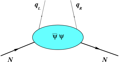
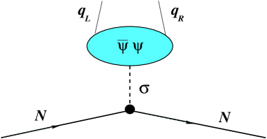
a		b

Figure 1: a. The oversimplified partonic interpretation of $e^{q}(x)$. b. The symbolic diagrammatic interpretation of the $\delta(x)$ contribution to $e^{a}(x)$ as suggested by Eq. (58). The quark-lines “carry the fraction $x=0$ of the nucleon momentum”, see text.

How to interpret a $\delta$-function?

A $\delta(x)$-contribution to a distribution function has no partonic interpretation. The observation in (58), however, suggests an intuitively appealing “interpretation”.

Oversimplifyingly $e^{a}(x){\rm d}x$ can be interpreted as taking out of the nucleon in the infinite momentum frame, e.g., a left-handed good light-cone quark component which carries between $x$ and $x+{\rm d}x$ of the nucleon momentum, and then reinserting a right-handed bad light-cone quark component with the same momentum back into the nucleon, see Fig. 1a. (The good and bad quark light-cone degrees of freedom are strictly speaking defined in the light-cone quantization. Good means independent degrees of freedom, the bad quark degrees of freedom are composites of good quark and gluon degrees of freedom. Considering this one obtains the correct partonic interpretation of $e^{a}(x)$ as a quark-gluon-quark correlation function Jaffe:1991kp ; Jaffe:1991ra .)

Does it make sense to pick up hereby a quark (or antiquark) which carries the fraction $x=0$ of the nucleon momentum, i.e. which is at rest with respect to the fast moving nucleon? Eq. (58) suggests that such a quark (or antiquark) is picked up from the vacuum, which to a certain extent is present also inside the nucleon. It should be stressed that one does not deal with a disconnected diagram. The factor $B_{sol}$ shows that the nucleon line and the vacuum blob are connected by the exchange of a resonance with the quantum numbers of the sigma meson, see the symbolic diagram in Fig. 1b.

It would be interesting to see whether such an “interpretation” could be confirmed by observations analogue to (58) in other models.

IV.3 Discussion of the results for $(e^{u}+e^{d})(x)$

The final result for $(e^{u}+e^{d})(x)$ from the interpolation formula is the contribution of the discrete level (31), (already the total result for $x\neq 0$) and the continuum contribution (58) consisting of a $\delta(x)$-function. It should be noted that there is no freedom to also regularize the UV-finite discrete level contribution in the Pauli-Villars regularization method. This contribution must not be regularized fore otherwise the variational problem of minimizing the soliton energy in (16) has no solution, i.e. no soliton exists Weiss:1997rt .

Fig. 2a shows the final results for $(e^{u}+e^{d})(x)$ and $(e^{\bar{u}}+e^{\bar{d}})(x)$ (no effort is made to indicate the $\delta$-function at $x=0$). It is instructive to compare $(e^{u}+e^{d})(x)$ to $(f_{1}^{u}+f_{1}^{d})(x)$ in the model. Both are of the same order in the large $N_{c}$-limit and become equal in the non-relativistic limit (see Sec. V). For the quarks one observes that $(f_{1}^{u}+f_{1}^{d})(x)$ is about 2-3 times larger than $(e^{u}+e^{d})(x)$, while the corresponding antiquark distributions are of a similar magnitude, see Figs. 2b and 2c.

a	b	c

Figure 2: a. The regular part of the chirally odd twist-3 flavour-singlet quark and antiquark distribution functions, $(e^{u}+e^{d})(x)$ and $(e^{\bar{u}}+e^{\bar{d}})(x)$, at a low normalization point of the model of about $600\,{\rm MeV}$ vs. $x$. At $x=0$ there is a $\delta(x)$-contribution. b. The chiral quark-soliton model results for $(e^{u}+e^{d})(x)$ (computed here) and $(f_{1}^{u}+f_{1}^{d})(x)$ (from Weiss:1997rt ) at a low scale of about $600\,{\rm MeV}$ vs. $x$. c. The same as Fig. 2b but for antiquarks.

In order to compute the coefficient $C$ of the $\delta(x)$-function in Eq. (58), one has to evaluate $B_{sol}$ (36). For the physical situation with $m_{\pi}=140\,{\rm MeV}$ one obtains

$$B_{sol}=\frac{1}{2}\int\!{\rm d}^{3}{\bf x}\,{\rm tr}_{\mbox{\tiny F}}\biggl{(}\frac{U+U^{\dagger}\!}{2}-1\biggr{)}=\int\!{\rm d}^{3}{\bf x}\,\biggl{(}\cos P(r,m_{\pi})-1\biggr{)}=-17.2\;R^{3}_{sol}\;.$$ (59)

In the chiral limit $m_{\pi}\to 0$ the integral in the expression for $B_{sol}$ in (36) can be evaluated in an elementary way yielding $B_{sol}=-2\sqrt{2}\,\pi^{2}R^{3}_{sol}=-27.9\,R^{3}_{sol}$. I.e. the coefficient $C$ is by about $40\%$ increased in the chiral limit. This demonstrates the importance of considering this quantity in the physical situation with finite $m_{\pi}$. Numerically one obtains for $R_{sol}=M^{-1}=(350\,{\rm MeV})^{-1}$ and $m_{\pi}=140\,{\rm MeV}$ the result

$$C=(9.1\pm 2.8)\;,$$ (60)

where the error is due to the uncertainty of the vacuum condensate $(-280\pm 30)^{3}{\rm MeV}^{3}$ Gasser:1982ap . For the first moment of $(e^{u}+e^{d})(x)$ one thus obtains

$$\int\limits_{-1}^{1}\!\!{\rm d}x\;(e^{u}+e^{d})(x)=\int\limits_{-1}^{1}\!\!{\rm d}x\;(e^{u}+e^{d})(x)_{\rm lev}+\int\limits_{-1}^{1}\!\!{\rm d}x\;(e^{u}+e^{d})(x)_{\rm cont}=1.6+(9.1\pm 2.8)=(10.7\pm 2.8)$$ (61)

in good agreement with (9). In order to obtain $\sigma_{\mbox{\tiny$\pi$N}}$ from Eq. (61) it is convenient to use the Gell-Mann–Oakes–Renner relation

$$m_{\pi}^{2}f_{\pi}^{2}=-\,m\;\langle{\rm vac}|(\bar{\psi}_{u}\psi_{u}+\bar{\psi}_{d}\psi_{d})|{\rm vac}\rangle\;,$$ (62)

which holds in the effective theory (10) Christov:1995vm and allows to eliminate the uncertainty from the phenomenological value of the vacuum condensate in the continuum contribution to $\sigma_{\mbox{\tiny$\pi$N}}$

$$(\sigma_{\mbox{\tiny$\pi$N}})_{\rm cont}=m\int_{-1}^{1}{\rm d}x\;(e^{u}+e^{d})(x)_{\rm cont}=m\,C=-m_{\pi}^{2}f_{\pi}^{2}\;B_{\rm sol}=67.8\,{\rm MeV}.$$ (63)

In order to obtain the contribution of the discrete level to $\sigma_{\mbox{\tiny$\pi$N}}$ one can use (62) to obtain a consistent value for the current quark mass $m=(8.2\pm 2.5)\,{\rm MeV}$. This yields $(\sigma_{\mbox{\tiny$\pi$N}})_{\rm lev}=(13.2\pm 4.1)\;{\rm MeV}$ and the total result is $\sigma_{\mbox{\tiny$\pi$N}}=(81\pm 4)\;{\rm MeV}$. There is no point in keeping track of the error in this case, since it is smaller than the accuracy of the interpolation formula (which was found to be about $\pm 10\%$ whenever it was checked quantitatively). Thus one obtains

$$\sigma_{\mbox{\tiny$\pi$N}}=81\;{\rm MeV}\;.$$ (64)

The result (63) is about $30\%$ larger than former exact results from the $\chi$QSM which, however, have been calculated with a different (proper-time) regularization Diakonov:1988mg ; Kim:1995hu . Considering that $\sigma_{\mbox{\tiny$\pi$N}}$ is quadratically divergent and thus rather strongly sensitive to regularization, the result in (64) is in good agreement with the results of Refs. Diakonov:1988mg ; Kim:1995hu . Worthwhile mentioning is that all model numbers – from Eq. (64) and from Refs. Diakonov:1988mg ; Kim:1995hu – are consistent with the phenomenological value for $\sigma_{\mbox{\tiny$\pi$N}}$ in Eq. (8) within $(10-30)\%$.

In QCD – as mentioned in Sec. II – the first moment of $e^{a}(x)$ is due to the $\delta(x)$-function only. In the $\chi$QSM the $\delta(x)$-function provides the dominant (more than $80\%$) but not the only contribution to the first Mellin moment of $(e^{u}+e^{d})(x)$. The second moment of $(e^{u}+e^{d})(x)$ receives no contribution from the continuum and is due to the discrete level contribution only

$$\int_{-1}^{1}{\rm d}x\;x\,(e^{u}+e^{d})(x)=0.20\;.$$ (65)

This result would imply that the quarks bound in the soliton field have an effective mass $\beta M\sim 78\,{\rm MeV}$ (in the chiral limit), see the discussion below (29, 30).

A comment is in order on an exact numerical evaluation of $(e^{u}+e^{d})(x)$. The distribution functions computed in the $\chi$QSM so far were all either UV-finite or at most logarithmically divergent. In the latter case always a single Pauli-Villars subtraction was sufficient. The regularization prescription (49, 50) precisely states how $(e^{u}+e^{d})(x)$ can practically be regularized. However, an exact numerical evaluation meets the problem to evaluate the model expressions for a Pauli-Villars mass $M_{2}\approx$ several ${\rm GeV}$ (see footnote 4) In the numerical calculation the spectrum of the Hamiltonian (14) is discretized and made finite (see e.g.  Diakonov:1997vc and references therein). For the latter step one considers only quark momenta below some large numerical cutoff $\Lambda_{\rm num}$ chosen much larger than any other (physical or numerical) scale involved in the problem. So far $\Lambda_{\rm num}\approx(8-10)\,{\rm GeV}$ was sufficient, but this is the order of magnitude of the second Pauli-Villars mass $M_{2}$. To compute $(e^{u}+e^{d})(x)$ one has to choose $\Lambda_{\rm num}$ much larger than $M_{2}$, which would result in an uneconomically large increase of computing time.

Interestingly, the singular $\delta(x)$-contribution would conceptually cause no problem for the numerical method of Ref. Diakonov:1997vc . The descretized spectrum of the Hamiltonian (14) yields discontinuous (distribution) functions of $x$. In Diakonov:1997vc it was proposed to smear the distribution functions $q(x)$, i.e. to convolute them with a narrow Gaussian with an appropriately chosen width $\gamma$ as $q(x)_{\rm smear}=$ $\frac{1}{\gamma\pi^{1/2}}\int{\rm d}x^{\prime}\exp(-\frac{(x-x^{\prime})^{2}}{\gamma^{2}})q(x^{\prime})$. (The smearing can be removed by a deconvolution procedure.) This trick would turn the $\delta(x)$-contribution in $(e^{u}+e^{d})(x)$ into a narrow-Gausssian with the well-defined width $\gamma$. In this way the coefficient of the $\delta(x)$-contribution could be well determined from the numerical result.

Finally, a comment is in order on (26) which relates the logarithmically divergent nucleon mass $M_{\mbox{\tiny N}}$ and the quadratically divergent $\sigma_{\mbox{\tiny$\pi$N}}$. $M_{\mbox{\tiny N}}$ requires a single Pauli-Villars subtraction, while $\sigma_{\mbox{\tiny$\pi$N}}$ requires two subtractions. Thus the quantities on the left-hand and right-hand side in (26) are regularized differently. In the Pauli-Villars regularization scheme the relation (26) has to be considered as formally correct modulo regularization effects. (Some other ambiguities in the Pauli-Villars regularization scheme were mentioned in Kubota:1999hx .) In other regularization methods – such as the proper time regularization – there are no such ambiguities.

IV.4 Comparison to the bag model

Figure 3: The twist-3 distribution function $(e^{u}+e^{d})(x)$ from the $\chi$QSM (solid line, obtained here) and from the bag model (dashed line, from Ref. Jaffe:1991ra ) vs. $x$. The meaning of the curves at negative $x$ is explained in Eq. (1). The $\chi$QSM result refers to a scale of about $0.6\,{\rm GeV}$. The bag model result refers to a scale of about $0.4\,{\rm GeV}$.

Studies of $e^{a}(x)$ were also performed in the framework of the bag model in Refs. Jaffe:1991ra ; Signal:1997ct . In Fig. 3 the $\chi$QSM result for the regular part of $(e^{u}+e^{d})(x)$ is compared to the result from the MIT bag model from Ref. Jaffe:1991ra . (For that the flavour-independent results for “$e(x)$” from Refs. Jaffe:1991ra are multiplied by the factor $N_{c}=3$ in order to compare to $(e^{u}+e^{d})(x)$ obtained here.) The comparison of the position of the maxima of the curves for quark distributions from the two models indicates that the bag model results refer to a somehow lower scale than $0.6\,{\rm GeV}$, the scale of the $\chi$QSM. (In Signal:1997ct the value of $0.4\,{\rm GeV}$ was quoted.) Taking this into account one concludes that both models give qualitatively similar results for quark distributions.

Concerning antiquarks the difference is more pronounced. However, the bag model description of antiquark distributions cannot be considered as reliable. A drawback of the bag model in this context is that it yields negative $f_{1}^{\bar{q}}(x)$ in contradiction to the positivity requirement.

V $e^{a}(x)$ in the non-relativistic limit

In the limit of the soliton size $R_{sol}\to 0$ the expressions of the $\chi$QSM go into the results of the non-relativistic (“naive”) quark model formulated for an arbitrary number of colours $N_{c}$ Karl:cz . In this sense the limit $R_{sol}\to 0$ corresponds to the non-relativistic limit in the $\chi$QSM. This was studied in detail in Ref. Praszalowicz:1995vi .

As $R_{sol}\to 0$ the soliton profile (18) goes to zero, and the $U$-field approaches unity. Correspondingly, the spectrum of the Hamiltonian (14) becomes more and more similar to that of the free Hamiltonian (15). Considering vacuum subtraction it is clear that the contribution of the continuum vanishes in this limit Praszalowicz:1995vi , and all that remains is the contribution of the discrete level $|{\rm lev}\rangle$. More precisely, as $R_{sol}\to 0$ the energy of the discrete level $E_{\rm lev}\to M$ (so the nucleon mass, (16), formally $M_{\mbox{\tiny N}}\to N_{c}E_{\rm lev}\to N_{c}M$), and the lower component of the Dirac-spinor of the discrete level wave-function goes to zero Praszalowicz:1995vi .

The limit $R_{sol}\to 0$ means that $U\to 1$ i.e. ${\rm log}\,U\ll 1$ which is the case (iii) in which the interpolation formula yields exact results (see Section IV.2). The first feature – in this case the vanishing of the continuum contribution in (32, 33) – can be observed in the final result $(e^{u}+e^{d})(x)_{\rm cont}=C\,\delta(x)$ in Eq. (58). The factor $B_{sol}$ in the coefficient $C$ vanishes with $R_{sol}\to 0$ as can be seen from its definition (36) or Eq. (59). Thus, in the non-relativistic limit the contribution of the $\delta$-function at $x=0$ vanishes because the coefficient $C$ goes to zero.

To study the non-relativistic limit in the discrete level contribution it is convenient to use the first expression in Eq. (31). Since only the upper component of the Dirac-spinor of the discrete level wave-function survives the limit Praszalowicz:1995vi , one can replace $\gamma^{0}$ by the unity matrix, i.e.

$$\lim\limits_{\mbox{\tiny non-rel}}(e^{u}+e^{d})(x)\longrightarrow N_{c}M_{\mbox{\tiny N}}\langle{\rm lev}|\delta(xM_{\mbox{\tiny N}}-\hat{p}^{3}-E_{\rm lev})|{\rm lev}\rangle\;.$$ (66)

Next consider that $E_{\rm lev}\to M$ and $M_{\mbox{\tiny N}}\to N_{c}M$ while the momenta of the non-relativistic quarks $|p^{i}|\ll M$ such that the corresponding operator in the $\delta$-function in (66) can be neglected. Using the normalization $\langle{\rm lev}|{\rm lev}\rangle=1$ one obtains

$$\lim\limits_{\mbox{\tiny non-rel}}(e^{u}+e^{d})(x)\longrightarrow N_{c}\,\delta\biggl{(}x-\frac{1}{N_{c}}\biggr{)}\;.$$ (67)

The first two moments of (67) read

$$\lim\limits_{\mbox{\tiny non-rel}}\int\limits_{-1}^{1}\!\!{\rm d}x\;(e^{u}+e^{d})(x)=N_{c} \lim\limits_{\mbox{\tiny non-rel}}\int\limits_{-1}^{1}\!\!{\rm d}x\;x\,(e^{u}+e^{d})(x)=1\;.$$ , (68)

To see that the relations (68) are the correct non-relativistic results for the QCD sum rules (4) and (6) one has to consider that in the non-relativistic limit the current quark mass $m\to M=M_{\mbox{\tiny N}}/N_{c}$ and $\sigma_{\mbox{\tiny$\pi$N}}\to M_{\mbox{\tiny N}}$. (The latter relation follows formally, e.g., from the Feynman-Hellmann theorem (26) with $m=M=M_{\mbox{\tiny N}}/N_{c}$.)

The twist-2 unpolarized flavour-singlet distribution function $(f_{1}^{u}+f_{1}^{d})(x)$ is given in the $\chi$QSM by Diakonov:1996sr

$$(f_{1}^{u}+f_{1}^{d})(x)=N_{c}M_{\mbox{\tiny N}}\sum\limits_{n\,\rm occ}\langle n|(1+\gamma^{0}\gamma^{3})\,\delta(xM_{\mbox{\tiny N}}-p^{3}-E_{n})|n\rangle\;,$$ (69)

i.e.  the only difference to $(e^{u}+e^{d})(x)$ is the different Dirac-structure $(1+\gamma^{0}\gamma^{3})$ instead of $\gamma^{0}$. This difference becomes irrelevant in the non-relativistic limit (where only the upper component of the Dirac-spinor of the discrete level wave-function survives) such that in this limit $(e^{u}+e^{d})(x)$ and $(f_{1}^{u}+f_{1}^{d})(x)$ become equal. This argument holds also for separat flavours and allows to generalize

$$\lim\limits_{\mbox{\tiny non-rel}}e^{q}(x)=\lim\limits_{\mbox{\tiny non-rel}}f_{1}^{q}(x)=N_{q}\,\delta\biggl{(}x-\frac{1}{N_{c}}\biggr{)}\;,$$ (70)

where $N_{q}$ denotes the number of the respective valence quarks (i.e. for the proton $N_{u}=2$ and $N_{d}=1$ for $N_{c}=3$ colours). The result (70) means that in the non-relativistic limit $e^{q}(x)$ is given by the mass term contribution in the decomposition (2) because

$$\lim\limits_{\mbox{\tiny non-rel}}\biggl{\{}\frac{m_{q}}{M_{\mbox{\tiny N}}}\;\frac{f_{1}^{q}(x)}{x}\biggr{\}}=\frac{M}{M_{\mbox{\tiny N}}}\lim\limits_{\mbox{\tiny non-rel}}\biggl{\{}\frac{f_{1}^{q}(x)}{x}\biggr{\}}=\lim\limits_{\mbox{\tiny non-rel}}f_{1}^{q}(x)\;.$$ (71)

In the intermediate step in (71) the $\delta(x-1/N_{c})$-function was used to replace $x$ in the denominator by $1/N_{c}$. One may worry that the large value $\sigma_{\mbox{\tiny$\pi$N}}=M_{\mbox{\tiny N}}$ would mean a large strangeness content of the nucleon. However, as discussed in Efremov:2002qh the value $\sigma_{\mbox{\tiny$\pi$N}}=M_{\mbox{\tiny N}}$ correctly implies a vanishing strangeness contribution to the nucleon mass in the non-relativistic limit.

Thus, though phenomenologically it is not satisfactory, the non-relativistic picture of the twist-3 distribution function $e^{q}(x)$ is consistent. In this limit the singular and pure twist-3 contributions in the decomposition (2) vanish, and $e^{q}(x)$ is given by the mass-term. Thus the chirally odd nature of $e^{q}(x)$ arises from a “mass insertion” into a quark line. Moreover, $e^{q}(x)$ and $f_{1}^{q}(x)$ become equal in this limit, and are trivial $\delta$-functions concentrated at $x=1/N_{c}$ which means that the nucleon momentum is distributed equally among the $N_{c}$ massive and non-interacting constituent quarks.

The usefulness of results of the kind (70) is best illustrated by the popularity of the non-relativistic relation between the twist-2 helicity $g_{1}^{q}(x)$ and transversity $h_{1}^{q}(x)$ distribution functions (here for $N_{c}=3$)

$$\lim\limits_{\mbox{\tiny non-rel}}h_{1}^{q}(x)=\lim\limits_{\mbox{\tiny non-rel}}g_{1}^{q}(x)=P_{q}\,\delta\biggl{(}x-\frac{1}{3}\biggr{)}\;,\;\;\;P_{u}=\frac{4}{3}\;,\;\;\;P_{d}=-\,\frac{1}{3}\;,$$ (72)

which yields for the axial charges $g_{A}^{(3)}=\frac{5}{3}$ and $g_{A}^{(0)}=1$. Though also these numbers are phenomenologically not fully satisfactory the assumption that $h_{1}^{a}(x)=g_{1}^{a}(x)$ at some low scale is a popular guess to estimate effects of transversity distribution, see Barone:2001sp for a review.

VI Summary and conclusions

A study of the flavour-singlet twist-3 distribution function $(e^{u}+e^{d})(x)$ in the $\chi$QSM was presented. It was shown that the model expressions are quadratically and logarithmically UV-divergent and can be regularized by the Pauli-Villars method. The model expressions for the quark and antiquark distribution functions $(e^{u}+e^{d})(x)$ and $(e^{\bar{u}}+e^{\bar{d}})(x)$ were evaluated using an approximation – the interpolation formula which in general well approximates exact model calculations.

The remarkable result is that the $\chi$QSM-expression for $(e^{u}+e^{d})(x)$ contains a $\delta$-function-type singularity at $x=0$ as expected from QCD Efremov:2002qh . This result is obtained here from a non-perturbative model calculation. Previously a $\delta(x)$-contribution in $e^{a}(x)$ was observed in a perturbative calculation in Ref. Burkardt:2001iy .

In the $\chi$QSM the coefficient of the $\delta$-function is proportional to the quark vacuum condensate. This is natural from the point of view that in QCD the singular contribution to $e^{q}(x)$ and the quark vacuum condensate are both the expectation values of the same local scalar operator, $\bar{\psi}_{q}(0)\psi_{q}(0)$, taken respectively in the nucleon and vacuum states. This observation allows to make a heuristic but physically appealing interpretation of the $\delta(x)$-contribution.

At $x\neq 0$ the $\chi$QSM yields results for $(e^{u}+e^{d})(x)$ similar to those obtained in the bag model at a comparably low scale Jaffe:1991ra ; Signal:1997ct . Both models suggest that $e^{a}(x)$ is sizable at low scales. The discription of $(e^{u}+e^{d})(x)$ in the $\chi$QSM is consistent in the sense that the sum rules for the first and the second moment are satisfied. However, in the $\chi$QSM the $\delta(x)$-contribution provides the dominant but not the only contribution to the first moment of $(e^{u}+e^{d})(x)$ unlike in QCD, and in the case of the second moment it is necessary to interpret the result correspondingly by introducing the notion of an effective quark mass. It would be interesting to see whether the failure of the bag model to satisfy the sum rule for the second moment reported in Jaffe:1991ra could also be reinterpreted in a similar spirit.

In effective models, such as $\chi$QSM or bag model, equations of motions are altered compared to QCD and there is no gauge principle which would allow to cleanly decompose $e^{a}(x)$ into a $\delta(x)$-contribution, a pure twist-3 part and a mass-term. Therefore one cannot expect that the QCD sum rules which are derived by means of the QCD equations of motion are literally satisfied in such models. Still within the models the results are consistent.

The (large-$N_{c}$) non-relativistic limit of $e^{q}(x)$ was studied on the basis of the $\chi$QSM expressions. It was found that in this limit $e^{q}(x)=f_{1}^{q}(x)$. The non-relativistic description of $e^{q}(x)$ was shown to be consistent.

The results and interpretations presented here should be reexamined in the more general framework of the instanton model of the QCD vacuum, on which the $\chi$QSM is founded. This was out of the scope of the study presented here and will be reported elsewhere.

Note added in Proof: After this work has been completed the work Wakamatsu:2003uu appeared, where the authors conclude the existence of a $\delta(x)$ contribution in $(e^{u}+e^{d})(x)$ in the chiral quark-soliton model in an independent and complementary way.

References

- (1) R. L. Jaffe and X. D. Ji, Phys. Rev. Lett. 67, 552 (1991).
- (2) R. L. Jaffe and X. D. Ji, Nucl. Phys. B 375, 527 (1992).
- (3) I. I. Balitsky, V. M. Braun, Y. Koike and K. Tanaka, Phys. Rev. Lett. 77, 3078 (1996).
- (4) A. V. Belitsky and D. Muller, Nucl. Phys. B 503, 279 (1997).
- (5) Y. Koike and N. Nishiyama, Phys. Rev. D 55, 3068 (1997).
- (6) A. V. Belitsky, in Proceedings of the “31st PNPI Winter School on Nuclear and Particle Physics”, St. Petersburg, Russia, 24 Feb - 2 Mar 1997, ed. V. A. Gordeev, pp.369-455 [arXiv:hep-ph/9703432].
- (7) J. Kodaira and K. Tanaka, Prog. Theor. Phys. 101, 191 (1999).
- (8) A. V. Efremov and P. Schweitzer, arXiv:hep-ph/0212044.
- (9) M. Burkardt and Y. Koike, Nucl. Phys. B 632, 311 (2002).
- (10) R. Koch, Z. Phys. C 15, 161 (1982).
- (11) M. M. Pavan, I. I. Strakovsky, R. L. Workman and R. A. Arndt, N Newsletter 16, 110 (2002) [arXiv:hep-ph/0111066].
-
(12)
J. C. Collins,
Nucl. Phys. B 396, 161 (1993).
X. Artru and J. C. Collins, Z. Phys. C 69, 277 (1996). -
(13)
D. Boer and P. J. Mulders, Phys. Rev. D57, 5780 (1998).
D. Boer, R. Jakob and P. J. Mulders, Phys. Lett. B424, 143 (1998).
D. Boer and R. Tangerman, Phys. Lett. B381, 305 (1996). - (14) A. V. Efremov, O. G. Smirnova and L. G. Tkachev, Nucl. Phys. Proc. Suppl. 74, 49 (1999); Nucl. Phys. Proc. Suppl. 79, 554 (1999). A. V. Efremov et al., Czech. J. Phys. 49, S75 (1999) [arXiv:hep-ph/9901216].
- (15) P. J. Mulders and R. D. Tangerman, Nucl. Phys. B461, 197 (1996) [Erratum-ibid. B484, 538 (1996)].
- (16) A. Airapetian et al. [HERMES Collaboration], Phys. Rev. Lett. 84, 4047 (2000); H. Avakian [HERMES Collaboration], Nucl. Phys. Proc. Suppl. 79, 523 (1999); A. Airapetian et al. [HERMES Collaboration], Phys. Rev. D 64, 097101 (2001).
- (17) H. Avakian [CLAS Collaboration], talk at 9th International Conference on the Structure of Baryons (Baryons 2002), Newport News, Virginia, 3-8 March 2002.
- (18) H. Avakian et al. [CLAS Collaboration], arXiv:hep-ex/0301005.
- (19) A. V. Efremov, K. Goeke and P. Schweitzer, Phys. Lett. B 522, 37 (2001) [Erratum-ibid. B 544, 389 (2002)].
- (20) A. V. Efremov, K. Goeke and P. Schweitzer, Acta Phys. Polon. B 33, 3755 (2002); and arXiv:hep-ph/0208124.
- (21) A. I. Signal, Nucl. Phys. B 497, 415 (1997).
- (22) D. I. Diakonov and V. Y. Petrov, Nucl. Phys. B 272, 457 (1986).
- (23) D. I. Diakonov and V. Y. Petrov, Nucl. Phys. B 245, 259 (1984).
- (24) D. I. Diakonov, M. V. Polyakov and C. Weiss, Nucl. Phys. B 461, 539 (1996).
- (25) D. I. Diakonov, V. Petrov, P. Pobylitsa, M. V. Polyakov and C. Weiss, Nucl. Phys. B 480, 341 (1996).
- (26) D. I. Diakonov, V. Y. Petrov, P. V. Pobylitsa, M. V. Polyakov and C. Weiss, Phys. Rev. D 56, 4069 (1997).
- (27) C. Weiss and K. Goeke, arXiv:hep-ph/9712447.
-
(28)
P. V. Pobylitsa and M. V. Polyakov,
Phys. Lett. B 389, 350 (1996);
P. V. Pobylitsa et al., Phys. Rev. D 59, 034024 (1999);
M. Wakamatsu and T. Kubota, Phys. Rev. D 60, 034020 (1999);
P. Schweitzer et al., Phys. Rev. D 64, 034013 (2001). - (29) K. Goeke, P. V. Pobylitsa, M. V. Polyakov, P. Schweitzer and D. Urbano, Acta Phys. Polon. B 32, 1201 (2001).
- (30) M. Glück, E. Reya and A. Vogt, Z. Phys. C 67, 433 (1995). M. Glück, E. Reya, M. Stratmann and W. Vogelsang, Phys. Rev. D 53, 4775 (1996).
- (31) J. Balla, M. V. Polyakov and C. Weiss, Nucl. Phys. B 510, 327 (1998).
- (32) B. Dressler and M. V. Polyakov, Phys. Rev. D61, 097501 (2000).
- (33) M. Wakamatsu, Phys. Lett. B 487, 118 (2000).
- (34) M. Wakamatsu, Phys. Lett. B 509, 59 (2001).
- (35) J. Gasser, H. Leutwyler and M. E. Sainio, Phys. Lett. B 253, 252 and 260 (1991).
- (36) T. Becher and H. Leutwyler, Eur. Phys. J. C 9, 643 (1999).
-
(37)
D. I. Diakonov, V. Y. Petrov and P. V. Pobylitsa,
Nucl. Phys. B 306, 809 (1988).
D. I. Diakonov and V. Y. Petrov, JETP Lett. 43, 75 (1986) [Pisma Zh. Eksp. Teor. Fiz. 43, 57 (1986)]. - (38) D. I. Diakonov and M. I. Eides, JETP Lett. 38, 433 (1983) [Pisma Zh. Eksp. Teor. Fiz. 38, 358 (1983)]; A. Dhar, R. Shankar and S. R. Wadia, Phys. Rev. D 31, 3256 (1985).
- (39) C. V. Christov et al., Prog. Part. Nucl. Phys. 37, 91 (1996).
-
(40)
V. Y. Petrov, P. V. Pobylitsa, M. V. Polyakov,
I. Börnig, K. Goeke and C. Weiss,
Phys. Rev. D 57, 4325 (1998);
M. Penttinen, M. V. Polyakov and K. Goeke, Phys. Rev. D 62, 014024 (2000);
P. Schweitzer, S. Boffi and M. Radici, Phys. Rev. D 66, 114004 (2002). - (41) E. Witten, Nucl. Phys. B 160, 57 (1979); E. Witten, Nucl. Phys. B 223, 433 (1983).
- (42) D. I. Diakonov, V. Y. Petrov and M. Praszałowicz, Nucl. Phys. B 323, 53 (1989).
- (43) H. C. Kim, A. Blotz, C. Schneider and K. Goeke, Nucl. Phys. A 596, 415 (1996).
- (44) J. Gasser and H. Leutwyler, Phys. Rept. 87, 77 (1982).
- (45) R. Delbourgo and M. D. Scadron, Mod. Phys. Lett. A 17, 209 (2002).
- (46) T. Kubota, M. Wakamatsu and T. Watabe, Phys. Rev. D 60, 014016 (1999).
- (47) G. Karl and J. E. Paton, Phys. Rev. D 30, 238 (1984).
- (48) M. Praszałowicz, A. Blotz and K. Goeke, Phys. Lett. B 354, 415 (1995).
- (49) V. Barone, A. Drago and P. G. Ratcliffe, Phys. Rept. 359, 1 (2002).
- (50) M. Wakamatsu and Y. Ohnishi, preprint OU-HEP-433, arXiv:hep-ph/0303007 (2003).