OCHA-PP-202 hep-ph/0302034

Neutrino Mass Matrix
Predicted From Symmetric Texture
Masako Bando and Midori Obara

¹ Aichi University, Aichi 470-0296, Japan

² Graduate School of Humanities and Sciences,
Ochanomizu University, Tokyo 112-8610, Japan

Within the framework of grand unified theories, we make full analysis of symmetric texture to see if such texture can reproduce large neutrino mixings, which have recently been confirmed by the observed solar and atmospheric neutrino oscillation experiments. It is found that so-called symmetric texture with anomalous $U(1)$ family symmetry with Froggatt-Nielsen mechanism does not provide a natural explanation of two large mixing angles. On the contrary we should adopt ”zero texture” which have been extensively studied by many authors and only this scenario can reproduce two large mixing angles naturally. Under such ”zero texture” with minimal symmetric Majorana matrix, all the neutrino masses and mixing angles, 6 quantities, are expressed in terms of up-quark masses, $m_{t},m_{c},m_{u}$ with two adjustable parameters. This provides interesting relations among neutrino mixing angles,

$$\tan^{2}2\theta_{12}\simeq\frac{144m_{c}}{m_{t}}\tan^{2}2\theta_{23}\cos^{2}\theta_{23},\quad\sin^{2}\theta_{13}\simeq\frac{4m_{c}}{m_{t}}\sin^{2}\theta_{23}\cos^{2}\theta_{12}.$$

Thus $|U_{e3}|$ is predicted to lie within the range $0.01-0.06$. Also absolute masses of three neutrinos are predicted almost uniquely. This is quite in contrast to the case where bi-large mixings come from the charged lepton sector with non-symmetric mass matrix, which does not provide the information of neutrino masses.

1 Introduction

Recent results from KamLAND [1] have completely excluded all the oscillation solutions for the solar neutrino except the Large Mixing Angle solution [2, 3, 4, 5]. This, combined with the present neutrino experiments by Super-Kamiokande [6, 7] and SNO [8] have confirmed neutrino oscillations with two large mixing angles [2, 9]:

$$\sin^{2}2\theta_{23}>0.83~{}(99\%~{}{\rm C.L.}),$$

$$0.29\leq\tan^{2}\theta_{12}\leq 0.86~{}(99.73\%~{}{\rm C.L.}).$$ (1.1)

The mass squared differences are [2, 10]

$$1.4\times 10^{-3}<\Delta m^{2}_{32}<6.0\times 10^{-3}~{}\rm{eV}^{2}~{}(99.73\%~{}{\rm C.L.}),$$ (1.2)

$$5.1\times 10^{-5}<\Delta m^{2}_{21}<9.7\times 10^{-5}~{}\rm{eV}^{2}~{}(99.73\%~{}{\rm C.L.}).$$ (1.3)

We are faced with a question; ” Why can such a large difference exist between the quark and lepton sectors? ” This is really a challenging question for any particle physicist who tries to find grand unified theories (GUTs).

These neutrino mixing angles are expressed in terms of MNS matrix [11];

$$V_{MNS}=U_{l}^{\dagger}U_{\nu},$$ (1.4)

with $U_{l}$ and $U_{\nu}$ being the unitary matrices which diagonalize the $3\times 3$ charged lepton and neutrino mass matrices, $M_{l}$ and $M_{\nu}$,

$$U_{l}^{\dagger}M_{l}^{\dagger}M_{l}U_{l} = {\rm diag}(m_{e}^{2},m_{\mu}^{2},m_{\tau}^{2}),$$ (1.5)

$$U_{\nu}^{\dagger}M_{\nu}^{\dagger}M_{\nu}U_{\nu} = {\rm diag}(m_{\nu_{1}}^{2},m_{\nu_{2}}^{2},m_{\nu_{3}}^{2}),$$ (1.6)

respectively. Here $M_{\nu}$ is calculated from right-handed Majorana neutrino mass matrix, $M_{R}$, and Dirac neutrino mass matrix, $M_{\nu_{D}}$,

$$M_{\nu}=M_{\nu_{D}}^{T}M_{R}^{-1}M_{\nu_{D}}.$$ (1.7)

If one want to derive such large mixings without any fine tuning, the origin of each of the large mixing angle, $\theta_{23}$ and $\theta_{12}$, must be due to either $M_{\nu}$ or $M_{l}$. In the GUT framework larger than $SU(5)$, if it includes Pati-Salam symmetry, we have not only a relation between down-type quark and charged lepton mass matrices, but also a relation between up-type quark and Dirac neutrino mass matrices. Thus if one attributes such large mixing angle of Eq. (1.4), either up-type or down-type quark mass matrix will give important information. To be more specific, let us adopt susy $SO(10)$ model which has now become more attractive since it unifies all the fermions of one family together with right-handed neutrino, $\nu_{R}$. Then once we fix each representation of Higgs field corresponding to each matrix element, $M_{l}$ and $M_{\nu_{D}}$ are uniquely determined from $M_{D}$ and $M_{U}$, respectively.

In this paper we make semi-empirical analysis on the case in which the origin of both those large mixing angles comes from the neutrino mass matrix. We here adopt the so-called symmetric four zero texture [12, 13] for up-quark mass matrix within susy $SO(10)$ GUT framework and examine if they are consistent with neutrino experiments with two large mixing angles. Here we assume that each elements of $M_{U}$ and $M_{D}$ is dominated by the contribution either from ${\bf 10}$ or ${\bf 126}$, the Yukawa coupling of charged lepton are that of the corresponding quark multiplied by $1$ or $-3$, respectively. More concretely, within symmetric texture the following option for $M_{D}$ has been known to reproduces charged lepton masses as well as down quark masses at the same time (Georgi-Jarlskog type [14, 15, 16, 17]);

$$M_{D}=\left(\begin{array}[]{@{\,}ccc@{\,}}0&{\bf 10}&0\\ {\bf 10}&{\bf 126}&{\bf 10}\\ 0&{\bf 10}&{\bf 10}\end{array}\right).$$ (1.11)

Now we examine which textures can be cnsistent with neutrino two large mixing angles. Among various options for configuration of ${\bf 10}$ or ${\bf 126}$, the following option has been found to be the best type which is consistent with the present neutrino experiments,

$$M_{U}=\left(\begin{array}[]{@{\,}ccc@{\,}}0&{\bf 126}&0\\ {\bf 126}&{\bf 10}&{\bf 10}\\ 0&{\bf 10}&{\bf 126}\end{array}\right).$$ (1.15)

This may be compared with Georgi-Jarlskog texture of down-type quark mass matrix of the above. Further remarkable fact is that once we fix a proprer option, the most economical Majorana neutrino mass matrix with two parameters can reproduce all the masses and mixing angles of neutrinos consistently with present experiments; even the order 1 coefficients are almost uniquely determined from the up-type quark masses only. In the next section we make general consideration on symmetric texture. We shall see that such mass matrix as derived from anomalous $U(1)$ family quantum assignment cannot naturally reproduce large mixing angles. According to this fact we here adopt the symmetric four zero texture. In section 3 we make numerical calculations and examine various cases. We obtain a good candidate for the types of configuration, which is investigated in section 4. Section 5 is devoted to further discussions.

2 Symmetric Texture

Symmetric texture for fermion mass matrices has been extensively investigated by many authors [16, 18, 19]. First let us make an important comment on the Froggatt-Nielsen mechanism [20] using anomalous $U(1)$ family quantum numbers. This is actually an attractive idea for explaining hierarchy of mass matrices observed in quark sectors. However so far as we take symmetric textures, this $U(1)$ cannot naturally reproduce neutrino large mixing angles. This might seem to contradict the common understanding that we can get any matrix $M_{\nu}$ for any $M_{\nu_{D}}$ by choosing an appropriate $M_{R}$, namely $M_{R}=M_{\nu_{D}}M_{\nu}^{-1}M^{T}_{\nu_{D}}$. However this is only true if we make fine tuning.

In order to see this, let us take $M_{U}$ so that each generation of left- and right-handed neutrino has anomalous $U(1)$ charge. If we restrict ourselves to symmetric texture, namely the family structure of left-handed up-type fermions are the same as that of right-handed fermions, they have the same $U(1)$ charges, $x_{1},x_{2},x_{3}$, respectively. Then the Dirac neutrino mass matrix,

$$S_{\nu_{D}}\sim\left(\begin{array}[]{@{\,}ccc@{\,}}\lambda^{x_{1}+x_{1}}&\lambda^{x_{1}+x_{2}}&\lambda^{x_{1}+x_{3}}\\ \lambda^{x_{2}+x_{1}}&\lambda^{x_{2}+x_{2}}&\lambda^{x_{2}+x_{3}}\\ \lambda^{x_{3}+x_{1}}&\lambda^{x_{3}+x_{2}}&\lambda^{x_{3}+x_{3}}\end{array}\right)\sim\lambda^{x_{i}}\lambda^{x_{j}}\sim\left(\begin{array}[]{@{\,}c@{\,}}\lambda^{x_{1}}\\ \lambda^{x_{2}}\\ \lambda^{x_{3}}\end{array}\right)\cdot\left(\begin{array}[]{@{\,}ccc@{\,}}\lambda^{x_{1}}&\lambda^{x_{2}}&\lambda^{x_{3}}\end{array}\right).$$ (2.8)

If we write the inverse of $M_{R}$ as,

$$M_{R}^{-1}\sim\left(\begin{array}[]{@{\,}ccc@{\,}}D_{11}&D_{12}&D_{13}\\ D_{12}&D_{22}&D_{23}\\ D_{13}&D_{23}&D_{33}\end{array}\right),$$ (2.12)

we easily get the following form from Eq. (1.7),

$$[M_{\nu}]_{ij}\sim\lambda^{x_{i}}\left(\sum\lambda^{x_{k}}D_{kl}\lambda^{x_{l}}\right)\lambda^{x_{j}}\quad\rightarrow\quad M_{\nu}\sim\left(\sum D_{kl}\cdot\lambda^{x_{k}+x_{l}}\right)\cdot S_{\nu_{D}}.$$ (2.13)

This clearly indicates that the resultant matrix $M_{\nu}$ is always proportional to the original hierarchical mass matrix. Hence it is impossible to get neutrino large mixing angles unless the dominant term of some element vanishes accidentally by making fine tuning. This is true even if we adjust the order of scales in $M_{R}$. However if some matrix elements of Eq. (2.8) is equal to zero, namely if we take texture zero, it can yield large mixing angles in the neutrino mass matrix as we shall see below.

According to the above observation, we adopt the following semi-empirical textures for up- and down-type quark mass matrices at the GUT scale [19] ,

$$M_{D} = \left(\begin{array}[]{@{\,}ccc@{\,}}0&\sqrt{\frac{m_{d}m_{s}m_{b}}{m_{b}-m_{d}}}&0\\ \sqrt{\frac{m_{d}m_{s}m_{b}}{m_{b}-m_{d}}}&m_{s}&\sqrt{\frac{m_{d}m_{b}(m_{b}-m_{s}-m_{d})}{m_{b}-m_{d}}}\\ 0&\sqrt{\frac{m_{d}m_{b}(m_{b}-m_{s}-m_{d})}{m_{b}-m_{d}}}&m_{b}-m_{d}\end{array}\right)$$ (2.17)

$$\simeq m_{b}\left(\begin{array}[]{@{\,}ccc@{\,}}0&\frac{\sqrt{m_{d}m_{s}}}{m_{b}}&0\\ \frac{\sqrt{m_{d}m_{s}}}{m_{b}}&\frac{m_{s}}{m_{b}}&\sqrt{\frac{m_{d}}{m_{b}}}\\ 0&\sqrt{\frac{m_{d}}{m_{b}}}&1\end{array}\right),$$ (2.21)

which reproduces beautifully the down-quark masses and mixing as well as charged lepton masses by taking the configuration of Eq. (1.11). As for the up-quark mass matrix, which we need to get neutrino mass matrix, we also take the following form,

$$M_{U}\simeq m_{t}\left(\begin{array}[]{@{\,}ccc@{\,}}0&\frac{\sqrt{m_{u}m_{c}}}{m_{t}}&0\\ \frac{\sqrt{m_{u}m_{c}}}{m_{t}}&\frac{m_{c}}{m_{t}}&\sqrt{\frac{m_{u}}{m_{t}}}\\ 0&\sqrt{\frac{m_{u}}{m_{t}}}&1\end{array}\right)\equiv m_{t}\left(\begin{array}[]{@{\,}ccc@{\,}}0&a_{u}&0\\ a_{u}&b_{u}&c_{u}\\ 0&c_{u}&1\end{array}\right),$$ (2.28)

which, together with the down-type texture of Eq. (2.21), reproduces all the observed quark masses as well as CKM mixings. However we have not yet found so far which configuration of Higgs representations should be chosen to give proper neutrino masses and mixings. There are 16 textures as to which representation is dominated in each component.

Table 1: Classification of the up-type mass matrices, $M_{U}$ and $M_{\nu_{D}}$.

Type	Texture		type	Texture
$A_{1}$	$\left(\begin{array}[]{@{\,}ccc@{\,}}0&\textbf{126}&0\\ \textbf{126}&\textbf{126}&\textbf{126}\\ 0&\textbf{126}&\textbf{126}\end{array}\right)^{\mathstrut}_{\mathstrut}$		$A_{2}$	$\left(\begin{array}[]{@{\,}ccc@{\,}}0&\textbf{126}&0\\ \textbf{126}&\textbf{126}&\textbf{126}\\ 0&\textbf{126}&\textbf{10}\end{array}\right)^{\mathstrut}_{\mathstrut}$
$B_{1}$	$\left(\begin{array}[]{@{\,}ccc@{\,}}0&\textbf{10}&0\\ \textbf{10}&\textbf{126}&\textbf{126}\\ 0&\textbf{126}&\textbf{126}\end{array}\right)^{\mathstrut}_{\mathstrut}$		$B_{2}$	$\left(\begin{array}[]{@{\,}ccc@{\,}}0&\textbf{10}&0\\ \textbf{10}&\textbf{126}&\textbf{126}\\ 0&\textbf{126}&\textbf{10}\end{array}\right)^{\mathstrut}_{\mathstrut}$
$C_{1}$	$\left(\begin{array}[]{@{\,}ccc@{\,}}0&\textbf{126}&0\\ \textbf{126}&\textbf{10}&\textbf{126}\\ 0&\textbf{126}&\textbf{126}\end{array}\right)^{\mathstrut}_{\mathstrut}$		$C_{4}$	$\left(\begin{array}[]{@{\,}ccc@{\,}}0&\textbf{126}&0\\ \textbf{126}&\textbf{10}&\textbf{126}\\ 0&\textbf{126}&\textbf{10}\end{array}\right)^{\mathstrut}_{\mathstrut}$
$C_{2}$	$\left(\begin{array}[]{@{\,}ccc@{\,}}0&\textbf{10}&0\\ \textbf{10}&\textbf{10}&\textbf{126}\\ 0&\textbf{126}&\textbf{126}\end{array}\right)^{\mathstrut}_{\mathstrut}$		$C_{3}$	$\left(\begin{array}[]{@{\,}ccc@{\,}}0&\textbf{10}&0\\ \textbf{10}&\textbf{10}&\textbf{126}\\ 0&\textbf{126}&\textbf{10}\end{array}\right)^{\mathstrut}_{\mathstrut}$
$F_{1}$	$\left(\begin{array}[]{@{\,}ccc@{\,}}0&\textbf{126}&0\\ \textbf{126}&\textbf{126}&\textbf{10}\\ 0&\textbf{10}&\textbf{126}\end{array}\right)^{\mathstrut}_{\mathstrut}$		$F_{4}$	$\left(\begin{array}[]{@{\,}ccc@{\,}}0&\textbf{126}&0\\ \textbf{126}&\textbf{126}&\textbf{10}_{2}\\ 0&\textbf{10}&\textbf{10}\end{array}\right)^{\mathstrut}_{\mathstrut}$
$F_{2}$	$\left(\begin{array}[]{@{\,}ccc@{\,}}0&\textbf{10}&0\\ \textbf{10}&\textbf{126}&\textbf{10}\\ 0&\textbf{10}&\textbf{126}\end{array}\right)^{\mathstrut}_{\mathstrut}$		$F_{3}$	$\left(\begin{array}[]{@{\,}ccc@{\,}}0&\textbf{10}&0\\ \textbf{10}&\textbf{126}&\textbf{10}\\ 0&\textbf{10}&\textbf{10}\end{array}\right)^{\mathstrut}_{\mathstrut}$
$S_{1}$	$\left(\begin{array}[]{@{\,}ccc@{\,}}0&\textbf{126}&0\\ \textbf{126}&\textbf{10}&\textbf{10}\\ 0&\textbf{10}&\textbf{126}\end{array}\right)^{\mathstrut}_{\mathstrut}$		$S_{2}$	$\left(\begin{array}[]{@{\,}ccc@{\,}}0&\textbf{126}&0\\ \textbf{126}&\textbf{10}&\textbf{10}\\ 0&\textbf{10}&\textbf{10}\end{array}\right)^{\mathstrut}_{\mathstrut}$
$A_{3}$	$\left(\begin{array}[]{@{\,}ccc@{\,}}0&\textbf{10}&0\\ \textbf{10}&\textbf{10}&\textbf{10}\\ 0&\textbf{10}&\textbf{126}\end{array}\right)^{\mathstrut}_{\mathstrut}$		$A_{4}$	$\left(\begin{array}[]{@{\,}ccc@{\,}}0&\textbf{10}&0\\ \textbf{10}&\textbf{10}&\textbf{10}\\ 0&\textbf{10}&\textbf{10}\end{array}\right)^{\mathstrut}_{\mathstrut}$

All possible 16 types are listed in Table 1. Once we fix their types, the Dirac neutrino mass matrix is automatically determined as:

$$M_{\nu_{D}}=\left(\begin{array}[]{@{\,}ccc@{\,}}0&\ast a_{u}&0\\ \ast a_{u}&\ast b_{u}&\ast c_{u}\\ 0&\ast c_{u}&\ast\end{array}\right)\equiv m_{t}\left(\begin{array}[]{@{\,}ccc@{\,}}0&a&0\\ a&b&c\\ 0&c&d\end{array}\right),$$ (2.35)

with the Clebsch-Gordan (CG) coefficients $\ast$, $1$ or $-3$ according to the corresponding types (see Table 1). As for the right-handed Majorana mass matrix, to which only ${\bf 126}$ Higgs field couples, we assume the following simplest texture ,

$$M_{R}=v_{\bf 126}\left(\begin{array}[]{@{\,}ccc@{\,}}0&A_{R}&0\\ A_{R}&0&0\\ 0&0&D_{R}\end{array}\right)\equiv m_{R}\left(\begin{array}[]{@{\,}ccc@{\,}}0&r&0\\ r&0&0\\ 0&0&1\end{array}\right).$$ (2.42)

with two parameters, $m_{R}$ and $r$. Now our task is to examine which types in Table 1 can reproduce the neutrino masses and mixing angles consistent with the experimental data. The neutrino mass matrix is now straightforwardly calculated as,

$$M_{\nu}=M_{\nu_{D}}^{T}M_{\nu_{R}}^{-1}M_{\nu_{D}}=\left(\begin{array}[]{@{\,}ccc@{\,}}0&\frac{a^{2}}{r}&0\\ \frac{a^{2}}{r}&2\frac{ab}{r}+c^{2}&c(\frac{a}{r}+1)\\ 0&c(\frac{a}{r}+1)&d^{2}\end{array}\right)\frac{m_{t}^{2}}{m_{R}}.$$ (2.46)

where $a,b,c,d$ are proportional to $a_{u},b_{u},c_{u},1$ with coefficients $1$ or $-3$ according to the relevant Higgs multiplets ${\bf 10}$ and ${\bf 126}$, respectively.

First we estimate the order of magnitudes . We know that the order of the parameters in Eq. (2.46) above are $a\ll b\sim c\ll 1$. With this in mind we recognize that the first term of 2-3 element of $M_{\nu}$ in Eq. (2.46) should be of order of $d^{2}$, namely $ac/r\sim\mathcal{O}(d^{2})$, in order to get large mixing angle $\theta_{23}$. This fixes the value of $r$,

$$r\sim\frac{ac}{d^{2}}\sim*\sqrt{\frac{m_{u}^{2}m_{c}}{m_{t}^{3}}}\sim 10^{-7},$$ (2.47)

which is indeed the ratio of the the right-handed Majorana mass of 3rd generation to those of the first and second generations. At this stage we now come to almost the same situation as discussed by Kugo, Yoshioka and one of the present author [21]. If we use the neutrino Dirac masses estimated from the charged lepton masses, we would have had almost the same order of Majorana masses for the 3rd and 2nd generations. On the contrary the top quark mass is very huge compared with that of charm quark. This is why we need very tiny value $r$. Quite interesting is that the same tiny value $r$ provides a large 1-2 mixing angle! Furthermore this small value of $r$ is very welcome, as has discussed there [21]; the right-handed Majorana mass of the third generation must become of order of GUT scale while those of the first and second generations are of order $10^{8}$ GeV. This is quite favorable for the GUT scenario to reproduce the bottom-tau mass ratio.

Now the problem is whether we can naturally reproduce the mixing angle $\theta_{12}$ by the present textures. Note that at this stage, once we fix configuration type, we have no more arbitrary parameters except for overall scale $M_{R}$. With this $r$, $M_{\nu}$ is approximately written as,

$$M_{\nu}=\left(\begin{array}[]{@{\,}ccc@{\,}}0&\frac{a^{2}}{r}&0\\ \frac{a^{2}}{r}&\frac{2ab}{r}&\frac{ac}{r}\\ 0&\frac{ac}{r}&d^{2}\end{array}\right)\frac{m_{t}^{2}}{m_{R}}\equiv\left(\begin{array}[]{@{\,}ccc@{\,}}0&\beta&0\\ \beta&\alpha&h\\ 0&h&1\end{array}\right)\frac{d^{2}m_{t}^{2}}{m_{R}},$$ (2.54)

with

$$h=\frac{ac}{rd^{2}},\qquad\alpha=\frac{2ab}{rd^{2}},\qquad\beta=\frac{a^{2}}{rd^{2}}.$$ (2.55)

Since $\beta\ll\alpha$ and $h\sim\mathcal{O}(1)$, we can calculate all the neutrino masses and mixings approximately. First let us diagonalize the dominant term with respect to the 2-3 submatrix of Eq. (2.54). The rotation angle, $\theta_{23}$ is written as,

$$\tan^{2}2\theta_{23} = \frac{4h^{2}}{(1-\alpha)^{2}},$$ (2.56)

through which $M_{\nu}$ is now deformed as

$$\left(\begin{array}[]{@{\,}ccc@{\,}}0&\beta&0\\ \beta&\alpha&h\\ 0&h&1\end{array}\right)\quad\stackrel{{\scriptstyle\longrightarrow}}{{\theta_{23}}}\quad\left(\begin{array}[]{@{\,}ccc@{\,}}0&\beta\cos\theta_{23}&\beta\sin\theta_{23}\\ \beta\cos\theta_{23}&\lambda_{2}&0\\ \beta\sin\theta_{23}&0&\lambda_{3}\end{array}\right)$$ (2.57)

with

$$\lambda_{3} = \frac{\alpha+1+\sqrt{(\alpha-1)^{2}+4h^{2}}}{2}\equiv\lambda_{\nu_{3}},$$ (2.58)

$$\lambda_{2} = \frac{\alpha+1-\sqrt{(\alpha-1)^{2}+4h^{2}}}{2}.$$ (2.59)

From Eq. (2.56) we notice that $\alpha$ should be very close to 1 in order to get large mixing angle $\theta_{23}$. Since we know the experimental bound for $\theta_{23}$,

$$\sin^{2}2\theta_{23}>0.83,$$

we can define the following small value $\varepsilon$ as

$$\varepsilon^{2}\equiv\frac{(1-\alpha)^{2}}{4h^{2}}\leq 0.205.$$ (2.60)

Let us make a rough estimation using the up-quark masses at GUT scale within the error [22],

$$\alpha = \frac{2b}{c}=*\frac{2b_{u}}{c_{u}}=*\frac{2m_{c}}{\sqrt{m_{u}m_{t}}}\sim*\times(1.0-2.4),$$ (2.61)

$$\beta = \frac{\>a\>}{\>c\>}=*\frac{a_{u}}{c_{u}}=*\sqrt{\frac{m_{c}}{m_{t}}}\sim*\times(0.03-0.05).$$ (2.62)

Hence in order to be consistent with small value $\varepsilon$, the values of $\alpha$ must be close to 1, so the CG coefficient $*$ in $\alpha$ must be $1$, not $-3$ or $-1/3$. This requires that 2-2 and 2-3 components of $M_{U}$ must couple to a common Higgs representation. With this $\varepsilon$, we can approximately rewrite as follows:

$$\lambda_{3} \simeq 1+h-h\varepsilon,$$ (2.63)

$$\lambda_{2} \simeq 1-h-h\varepsilon.$$ (2.64)

Next step is to rotate with respect to the 1-2 submatrix of Eq. (2.57),

$$\tan^{2}2\theta_{12}=\Biggl{(}\frac{2\beta\cos\theta_{23}}{\lambda_{2}}\Biggr{)}^{2},$$ (2.65)

with which the neutrino mass matrix becomes

$$\stackrel{{\scriptstyle\longrightarrow}}{{\theta_{12}}}\quad\left(\begin{array}[]{@{\,}ccc@{\,}}\lambda_{\nu_{1}}&0&\beta\sin\theta_{23}\cos\theta_{12}\\ 0&\lambda_{\nu_{2}}&\beta\sin\theta_{23}\sin\theta_{12}\\ \beta\sin\theta_{23}\cos\theta_{12}&\beta\sin\theta_{23}\sin\theta_{12}&\lambda_{\nu_{3}}\end{array}\right),$$ (2.66)

with eigenvalues,

$$\lambda_{\nu_{2}} = \frac{\lambda_{2}+\sqrt{\lambda_{2}^{2}+4\beta^{2}\cos^{2}\theta_{23}}}{2},$$ (2.67)

$$\lambda_{\nu_{1}} = \frac{\lambda_{2}-\sqrt{\lambda_{2}^{2}+4\beta^{2}\cos^{2}\theta_{23}}}{2}.$$ (2.68)

Now in order to realize large mixing angle $\theta_{12}$ appearing in Eq. (2.65), $\lambda_{2}$ in Eq. (2.64) must become at least of the same order as $2\beta$. This requires again $h\sim 1$. It is not trivial that the same $h$ which gives large $\theta_{23}$ with the fixed values $\alpha$ and $\beta$ also produces large mixing angle $\theta_{12}$ at the same time. The larger the ratio $2\beta\cos\theta_{23}/\lambda_{2}$ is, the larger value of $\nu_{e}$-$\nu_{\mu}$ mixing we get. So it would be desired that $\beta$ must be as large as possible, namely the coefficient of $a_{u}$ in Eq. (2.35) may be desired to be $-3$ , which yields $\beta\sim-0.1$. In this way we have found the following conditions for the desired candidate for the type of Higgs representations.

Condition for Higgs configurations

1. The Higgs representations coupled with 2-3 and 2-2 elements of $M_{U}$ must be same.

2. The Higgs representation coupled with 1-2 elements of $M_{U}$ must be as large as possible.

As a result there remain the follwoing two types for most desirable candidates,

$$\left(\begin{array}[]{@{\,}ccc@{\,}}0&{\bf 126}&0\\ {\bf 126}&{\bf 10}&{\bf 10}\\ 0&{\bf 10}&{\bf 126}\end{array}\right),\qquad\left(\begin{array}[]{@{\,}ccc@{\,}}0&{\bf 126}&0\\ {\bf 126}&{\bf 10}&{\bf 10}\\ 0&{\bf 10}&{\bf 10}\end{array}\right).$$ (2.75)

Finally the neutrino masses are given as,

$$m_{\nu_{3}}\sim\lambda_{\nu_{3}}\frac{d^{2}m^{2}_{t}}{m_{R}},\quad m_{\nu_{2}}\sim\lambda_{\nu_{2}}\frac{d^{2}m^{2}_{t}}{m_{R}},\quad m_{\nu_{1}}\sim\lambda_{\nu_{1}}\frac{d^{2}m^{2}_{t}}{m_{R}}.$$ (2.76)

We should check if the same $h$ can also reproduce the two neutrino mass squared differences with one remaining parameter $m_{R}$. In the next section we make numerical calculation and see how the above observation can be actually confirmed.

3 Numerical Calculations

In this section we make numerical calculations for all the possible types for Higgs configuration. The forms of $h,\alpha,\beta$ are written in terms of $m_{t},m_{c},m_{u}$ with a parameter $r$ in Table 2. As our input we take the values of up-type quark masses, $m_{t},m_{c},m_{u}$ at GUT scale obtained by Fusaoka and Koide [22];

$$m_{u} = 1.04^{+0.19}_{-0.20}~{}{\rm MeV},$$ (3.1)

$$m_{c} = 302^{+25}_{-27}~{}{\rm MeV},$$ (3.2)

$$m_{t} = 129^{+196}_{-40}~{}{\rm GeV}.$$ (3.3)

Table 2: The forms of $h$, $\alpha$ and $\beta$ with the value of $d$ for each type.

Type	d	$h$ in $\frac{ac}{r}$ unit	$\alpha$ in $2m_{c}/\sqrt{m_{u}m_{t}}$ unit	$\beta$ in $\sqrt{m_{c}/m_{t}}$ unit
$S_{1}$	9	$-1/3$	$1$	$-3$
$S_{2}$	1	$-3$	$1$	$-3$
$A_{1}$	$1$	$1$	$1$	$1$
$A_{2}$	$1$	$9$	$1$	$1$
$A_{3}$	$9$	$1/9$	$1$	$1$
$A_{4}$	$1$	$1$	$1$	$1$
$B_{1}$	$9$	$-1/3$	$1$	$-1/3$
$B_{2}$	$1$	$-3$	$1$	$-1/3$
$C_{1}$	$9$	$1$	$-1/3$	$1$
$C_{2}$	$9$	$-1/3$	$-1/3$	$-1/3$
$C_{3}$	$1$	$-3$	$-1/3$	$-1/3$
$C_{4}$	$1$	$9$	$-1/3$	$1/9$
$F_{1}$	$9$	$-1/3$	$-3$	$-3$
$F_{2}$	$9$	$1/9$	$-3$	$9$
$F_{3}$	$1$	$1$	$-3$	$1$
$F_{4}$	$9$	$-3$	$-3$	$-3$

The present experimental data exists for the mixing angles $\theta_{23}$, $\theta_{12}$ , $\Delta m^{2}_{32}$ and $\Delta m^{2}_{21}$ with upper bound for $|U_{e3}|$. Of course, as we mentioned in the previous section, we could always reproduce the data $\theta_{23}$ by adjusting arbitrary parameter $h$ or equivalently $r$. However we already know that $h\sim\mathcal{O}(1)$ so we restrict $h$ not too far from 1, keeping the region from $0.3$ to $3.0$. Nontrivial is to reproduce large mixing angle $\theta_{12}$ since in principle we have no parameter at all, and only the freedom is the range of the quark masses at GUT scale of Eqs. (3.1)–(3.3), among which $m_{t}$ is the most sensitive parameter and at least known because of its large Yukawa coupling causing ambiguity via its evolution to the GUT scale. Within those parameter regions more than half of the types are excluded by experiments. Still surprising is that only the CG coefficients 3 or $-1/3$ does work well. Our model has no more arbitrary parameters and everything is fixed without any ambiguity. Thus if the errors of experimental data are improved, we can check more strictly whether or not our predictions agree with experiments. We calculate numerically the above quantities and compare them with the experimental data. According to Table 2, we classify 16 types into $S$, $A$, $B$, $C$ and $F$ classes.

3.1 Class $F$

This class does not satisfy the condition (i) of the previous section: the value of $\alpha$ is

$$\alpha\sim-6h\,\frac{m_{c}}{\sqrt{m_{u}m_{t}}}\sim(3.0-7.2)\,h,$$ (3.4)

which is far from 1. We calculate the atmospheric neutrino mixing angle, $\theta_{23}$. The class $F$ is those which does not reproduce large mixing at all, unless we take $h$ larger than $3.0$ where we can never reproduce large mixing angle $\theta_{12}$, as was mentioned in section 2. The calculated results are shown in Fig. 1 from which we confirm that solar neutrino mixing angle remain almost two order smaller than experimental bound. So we do not have large mixing for solar neutrinos even if we could adjust very large parameter $h$.

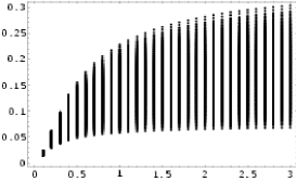
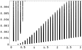
Figure 1: Calculated values of $\sin^{2}2\theta_{23}$ versus $h$ and $\tan^{2}\theta_{12}$ versus $h$ in class $F$.

3.2 Class $C$

Next for those which are classified by $C$, the value of $\alpha$ is

$$\alpha\sim-\frac{\>2\>}{3}h\,\frac{m_{c}}{\sqrt{m_{u}m_{t}}}\sim(0.3-0.8)\,h,$$ (3.5)

which is not so far from 1. This range of value makes better situation than the class $F$. We calculate then the solar neutrino mixing angle, $\theta_{12}$, and found that the class $C$ produces too small mixing angle. In order that 1-2 mixing of neutrino becomes large, $\lambda_{2}$ and $\beta$ have to be of the same order. The 2-2 element of $M_{\nu}$ in class $C$, namely $\alpha\sim(-2/3)\,b/c$ yields $\lambda_{2}\sim 0.1-0.5$. However, the value of $\beta$ is

$$\beta\sim h\,\sqrt{\frac{m_{c}}{m_{t}}}\sim(0.03-0.05)\,h,$$ (3.6)

which cannot become the same order as $\lambda_{2}$. Fig. 2 shows numerical results. We see that within the range $h\leq 3$, the values of $\sin^{2}2\theta_{23}$ become larger than 0.83. However such $h$ makes the values of $\tan^{2}\theta_{12}$ even smaller.

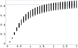
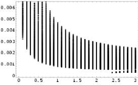
Figure 2: Calculated vales of $\sin^{2}2\theta_{23}$ versus $h$ and $\tan^{2}\theta_{12}$ versus $h$ in class $C$.

3.3 Class $B$

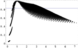
Figure 3: Calculated values of $\sin^{2}2\theta_{23}$ versus $h$ and $\sin^{2}2\theta_{23}$ versus $\alpha$ in class $B$.

This class satisfies the condition (i) and the value of $\alpha$ is

$$\alpha\sim 2h\,\frac{m_{c}}{\sqrt{m_{u}m_{t}}}\sim(1.0-2.4)\,h.$$ (3.7)

Fig. 3 indicates that the calculated results may reach to the bound of atmospheric neutrino mixing around $h\sim 1$. Since all the parameters are fixed within errors of the up-quark masses at GUT scales, we can express $\sin^{2}2\theta_{23}$ as a function of $\alpha$. The $\alpha$ dependence of $\sin^{2}2\theta_{23}$ is also seen in Fig. 3, from which we easily recognize that the values of $\sin^{2}2\theta_{23}$ becomes larger as $\alpha$ approaches closer to 1. Thus we can always adjust the parameter $h$ so that it reproduces the experimental data of $\sin^{2}2\theta_{23}$. However once we fix $h$, the type $B$ can hardly reproduce the value of mixing angle $\theta_{12}$ larger than the experimental bound 0.24.

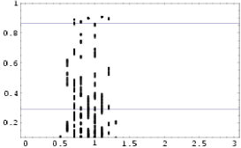
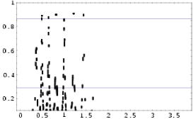
Figure 4: Calculated values of $\tan^{2}\theta_{12}$ versus $h$ and $\tan^{2}\theta_{12}$ versus $\alpha$ in class $B$.

This can be seen from Fig. 4. This is because this class does not satisfy the condition (ii) and the value of $\beta$ is

$$\beta\sim\,\frac{-h}{3}\sqrt{\frac{m_{c}}{m_{t}}}\sim(0.01-0.017)\,h,$$ (3.8)

which cannot become the same order as $\lambda_{2}$.

3.4 Class $A$

This class satisfies the condition (i) and (ii) and seems to be a little easier to reproduce large mixing angle $\theta_{12}$ than class $B$, since the value of $\beta$ is

$$\beta\sim\,\sqrt{\frac{m_{c}}{m_{t}}}\sim(0.03-0.05)\,h.$$ (3.9)

Fig. 5 indicates the $h$ dependence of $\sin^{2}2\theta_{23}$ as well as $\alpha$. The numerical results of solar neutrino mixing angle in Fig. 6 covers the present experimental allowed region rather well.

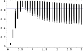
Figure 5: Calculated values of $\sin^{2}2\theta_{23}$ versus $h$ and $\sin^{2}2\theta_{23}$ versus $\alpha$ in class $A$.

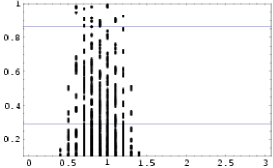
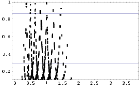
Figure 6: Calculated values of $\tan^{2}\theta_{12}$ versus $h$ and $\tan^{2}\theta_{12}$ versus $\alpha$ in class $A$.

We further calculate the mass squared differences for atmospheric and solar neutrinos, and the ratio of them, which are to be compared with the experimental results in Eqs. (1.2) and (1.3). These results are showed in Fig. 7 and 8.

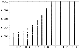
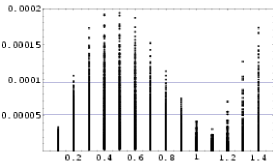
Figure 7: Calculated values of $\Delta m^{2}_{32}$ versus $h$ and $\Delta m^{2}_{21}$ versus $h$ in class $A$.

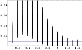
Figure 8: Calculated values of $\Delta m^{2}_{21}/\Delta m^{2}_{32}$ versus $h$ in class $A$.

3.5 Class $S$

Finally we have the class $S$ which satisfies both the conditions (i) and (ii) as well. This class is even easier to reproduce large mixing angle $\theta_{12}$ than class $A$, since the value of $\beta$ is

$$\beta\sim\,-3\sqrt{\frac{m_{c}}{m_{t}}}\sim(0.09-0.15)\,h.$$ (3.10)

Fig. 9 shows the calculated values of $\sin^{2}2\theta_{23}$ versus $h$ as well as $\alpha$ and Fig. 10 shows the $h$ and $\alpha$ dependence of $\tan^{2}\theta_{12}$. From Fig. 9 and Fig. 10, one finds the most probable region of $h$ is found within almost $1\pm 0.3$. We also show the figure of the calculated values of neutrino mass squared differences and their ratio (see Fig. 11 and Fig. 12). All the above results actually indicates that the type $S$ is excellently consistent with the present experimental bound.

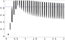
Figure 9: Calculated values of $\sin^{2}2\theta_{23}$ versus $h$ and $\sin^{2}2\theta_{23}$ versus $\alpha$ in class $S$.

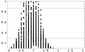
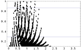
Figure 10: Calculated values of $\tan^{2}\theta_{12}$ versus $h$ and $\tan^{2}\theta_{12}$ versus $\alpha$ in class $S$.

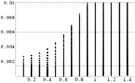
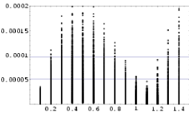
Figure 11: Calculated values of $\Delta m^{2}_{32}$ versus $h$ and $\Delta m^{2}_{21}$ versus $h$ in class $S$.

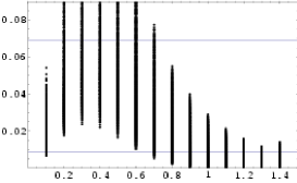
Figure 12: Calculated values of $\Delta m^{2}_{21}/\Delta m^{2}_{32}$ versus $h$ in class $S$.

3.6 Summary

Here we would like to summarize the range of parameters with which we can reproduce the experimental data for the possible candidates, the types $S$, $A$ and $B$ in Table 3, and the numerical results for the absolute masses of neutrinos and $|U_{e3}|$ in Table 4. Also we have summarized the situation of the type $C$ and $F$ which are not proper candidates at all (see Table 5).

Table 3: The neutrino properties for the types $S$, $A$ and $B$. $\bigcirc$ indicates that corresponding type can reproduce the experimental data, $\circledcirc$ even better, and $\triangle$ less probable. The values of $h$ which can reproduce both $\sin^{2}2\theta_{23}$ and $\tan^{2}\theta_{12}$ and $m_{R}$ which can reproduce both $\Delta m^{2}_{32}$ and $\Delta m^{2}_{21}$ are shown.

Type	Texture	$\sin^{2}2\theta_{23}$	$\tan^{2^{\mathstrut}}\theta_{12}$	$h$	$m_{R}~{}({\rm GeV})$
$S_{1}$	$\left(\begin{array}[]{@{\,}ccc@{\,}}0&\textbf{126}&0\\ \textbf{126}&\textbf{10}&\textbf{10}\\ 0&\textbf{10}&\textbf{126}\end{array}\right)^{\mathstrut}_{\mathstrut}$	$\bigcirc$	$\circledcirc$	$0.4-1.4$	$2\times 10^{15}$
$S_{2}$	$\left(\begin{array}[]{@{\,}ccc@{\,}}0&\textbf{126}&0\\ \textbf{126}&\textbf{10}&\textbf{10}\\ 0&\textbf{10}&\textbf{10}\end{array}\right)^{\mathstrut}_{\mathstrut}$	$\bigcirc$	$\circledcirc$	$0.4-1.4$	$2\times 10^{14}$
$A_{1}$	$\left(\begin{array}[]{@{\,}ccc@{\,}}0&\textbf{126}&0\\ \textbf{126}&\textbf{126}&\textbf{126}\\ 0&\textbf{126}&\textbf{126}\end{array}\right)^{\mathstrut}_{\mathstrut}$	$\bigcirc$	$\bigcirc$	$0.5-1.3$	$2\times 10^{15}$
$A_{2}$	$\left(\begin{array}[]{@{\,}ccc@{\,}}0&\textbf{10}&0\\ \textbf{10}&\textbf{10}&\textbf{10}\\ 0&\textbf{10}&\textbf{126}\end{array}\right)^{\mathstrut}_{\mathstrut}$	$\bigcirc$	$\bigcirc$	$0.5-1.3$	$2\times 10^{15}$
$A_{3}$	$\left(\begin{array}[]{@{\,}ccc@{\,}}0&\textbf{126}&0\\ \textbf{126}&\textbf{126}&\textbf{126}\\ 0&\textbf{126}&\textbf{10}\end{array}\right)^{\mathstrut}_{\mathstrut}$	$\bigcirc$	$\bigcirc$	$0.5-1.3$	$2\times 10^{14}$
$A_{4}$	$\left(\begin{array}[]{@{\,}ccc@{\,}}0&\textbf{10}&0\\ \textbf{10}&\textbf{10}&\textbf{10}\\ 0&\textbf{10}&\textbf{10}\end{array}\right)^{\mathstrut}_{\mathstrut}$	$\bigcirc$	$\bigcirc$	$0.5-1.3$	$2\times 10^{14}$
$B_{1}$	$\left(\begin{array}[]{@{\,}ccc@{\,}}0&\textbf{10}&0\\ \textbf{10}&\textbf{126}&\textbf{126}\\ 0&\textbf{126}&\textbf{126}\end{array}\right)^{\mathstrut}_{\mathstrut}$	$\bigcirc$	$\triangle$	$0.6-1.2$	$2\times 10^{15}$
$B_{2}$	$\left(\par\begin{array}[]{@{\,}ccc@{\,}}0&\textbf{10}&0\\ \textbf{10}&\textbf{126}&\textbf{126}\\ 0&\textbf{126}&\textbf{10}\end{array}\right)^{\mathstrut}_{\mathstrut}$	$\bigcirc$	$\triangle$	$0.6-1.2$	$2\times 10^{14}$

Table 4: The predicted values of $|m_{\nu_{3}}|$, $|m_{\nu_{2}}|$, $|m_{\nu_{1}}|$ and $|U_{e3}|$ for each type with $h$, $m_{R}$

Type	$h$	$m_{R}~{}({\rm GeV})$	$~{}~{}|m_{\nu_{3}}|^{\mathstrut}_{\mathstrut}~{}({\rm eV})~{}$	$~{}~{}|m_{\nu_{2}}|~{}({\rm eV})~{}$	$|m_{\nu_{1}}|~{}({\rm eV})$	$|U_{e3}|$
$S_{1}$	$0.4-1.4$	$2\times 10^{15^{\mathstrut}}$	$0.005-0.17$	$0.001-0.015$	$3\times 10^{-5}-4\times 10^{-3}$	$0.01-0.06$
$S_{2}$	$0.4-1.4$	$2\times 10^{14^{\mathstrut}}$	$0.005-0.17$	$0.001-0.015$	$3\times 10^{-5}-4\times 10^{-3}$	$0.01-0.06$
$A_{1}$	$0.5-1.3$	$2\times 10^{15^{\mathstrut}}$	$0.006-0.15$	$0.002-0.014$	$3\times 10^{-6}-1\times 10^{-3}$	$0.006-0.02$
$A_{2}$	$0.5-1.3$	$2\times 10^{15^{\mathstrut}}$	$0.006-0.15$	$0.002-0.014$	$3\times 10^{-6}-1\times 10^{-3}$	$0.006-0.02$
$A_{3}$	$0.5-1.3$	$2\times 10^{14^{\mathstrut}}$	$0.006-0.15$	$0.002-0.014$	$3\times 10^{-6}-1\times 10^{-3}$	$0.006-0.02$
$A_{4}$	$0.5-1.3$	$2\times 10^{14^{\mathstrut}}$	$0.006-0.15$	$0.002-0.014$	$3\times 10^{-6}-1\times 10^{-3}$	$0.006-0.02$
$B_{1}$	$0.6-1.2$	$2\times 10^{15^{\mathstrut}}$	$0.006-0.13$	$0.002-0.014$	$5\times 10^{-7}-3\times 10^{-3}$	$0.002-0.007$
$B_{2}$	$0.6-1.2$	$2\times 10^{14^{\mathstrut}}$	$0.006-0.13$	$0.002-0.015$	$6\times 10^{-7}-4\times 10^{-3}$	$0.002-0.007$

Table 5: The neutrino properties for the types $C$ and $F$. The notation $\bigcirc$ indicates that corresponding type can reproduce the experimental data and $\times$ impossible.

Type	Texture	$\sin^{2}2\theta_{23}$	$\tan^{2^{\mathstrut}}\theta_{12}$	$h$
$C_{1}$	$\left(\begin{array}[]{@{\,}ccc@{\,}}0&\textbf{126}&0\\ \textbf{126}&\textbf{10}&\textbf{126}\\ 0&\textbf{126}&\textbf{126}\end{array}\right)^{\mathstrut}_{\mathstrut}$	$\bigcirc$	$\times$	none
$C_{2}$	$\left(\begin{array}[]{@{\,}ccc@{\,}}0&\textbf{10}&0\\ \textbf{10}&\textbf{10}&\textbf{126}\\ 0&\textbf{126}&\textbf{126}\end{array}\right)^{\mathstrut}_{\mathstrut}$	$\bigcirc$	$\times$	none
$C_{3}$	$\left(\begin{array}[]{@{\,}ccc@{\,}}0&\textbf{10}&0\\ \textbf{10}&\textbf{10}&\textbf{126}\\ 0&\textbf{126}&\textbf{10}\end{array}\right)^{\mathstrut}_{\mathstrut}$	$\bigcirc$	$\times$	none
$C_{4}$	$\left(\begin{array}[]{@{\,}ccc@{\,}}0&\textbf{126}&0\\ \textbf{126}&\textbf{10}&\textbf{126}\\ 0&\textbf{126}&\textbf{10}\end{array}\right)^{\mathstrut}_{\mathstrut}$	$\bigcirc$	$\times$	none
$F_{1}$	$\left(\begin{array}[]{@{\,}ccc@{\,}}0&\textbf{126}&0\\ \textbf{126}&\textbf{126}&\textbf{10}\\ 0&\textbf{10}&\textbf{126}\end{array}\right)^{\mathstrut}_{\mathstrut}$	$\times$	$\times$	none
$F_{2}$	$\left(\begin{array}[]{@{\,}ccc@{\,}}0&\textbf{10}&0\\ \textbf{10}&\textbf{126}&\textbf{10}\\ 0&\textbf{10}&\textbf{126}\end{array}\right)^{\mathstrut}_{\mathstrut}$	$\times$	$\times$	none
$F_{3}$	$\left(\begin{array}[]{@{\,}ccc@{\,}}0&\textbf{10}&0\\ \textbf{10}&\textbf{126}&\textbf{10}\\ 0&\textbf{10}&\textbf{10}\end{array}\right)^{\mathstrut}_{\mathstrut}$	$\times$	$\times$	none
$F_{4}$	$\left(\begin{array}[]{@{\,}ccc@{\,}}0&\textbf{126}&0\\ \textbf{126}&\textbf{126}&\textbf{10}\\ 0&\textbf{10}&\textbf{10}\end{array}\right)^{\mathstrut}_{\mathstrut}$	$\times$	$\times$	none

In summarizing we have found that the best type for configuration which is consistent with the experiments is $S_{1}$. We shall discuss this type in detail in the next section.

4 Predictions of Type $S_{1}$

All the above results are summarized in Table 3 and Table 5, where all the 16 types are classified into 5 classes, $F,C,B,A$ and $S$. From these tables one sees that the class $S$ reproduces most naturally the large mixing angles for both atmospheric and solar neutrinos as well as the ratio of atmospheric to solar mass squared differences. The explicit forms of up-type mass matrix for the class $S$ are seen in Eq. (2.75), as we expected in section 2. Those two types yield the same predictions except for the Majorana mass scale. The type $S_{1}$ requires $m_{R}\sim 2\times 10^{15}~{}{\rm GeV}$ and in the type $S_{2}$, we have $m_{R}\sim 10^{14}~{}{\rm GeV}$, respectively. Thus more desirable one may be the type $S_{1}$ since it predicts more realistic bottom-tau ratio at low energy. Thus we here discuss the type $S_{1}$ in detail, namely we take,

$$M_{U}=\left(\begin{array}[]{@{\,}ccc@{\,}}0&{\bf 126}&0\\ {\bf 126}&{\bf 10}&{\bf 10}\\ 0&{\bf 10}&{\bf 126}\end{array}\right),$$ (4.4)

which determines $M_{\nu_{D}}$ as follows:

$$M_{\nu_{D}}=m_{t}\left(\begin{array}[]{@{\,}ccc@{\,}}0&-3a_{u}&0\\ -3a_{u}&b_{u}&c_{u}\\ 0&c_{u}&-3\end{array}\right).$$ (4.8)

With this Eq. (4.8), we obtain the neutrino mass matrix from Eq. (1.7),

$$M_{\nu}=\left(\begin{array}[]{@{\,}ccc@{\,}}0&\frac{a_{u}^{2}}{r}&0\\ \frac{a_{u}^{2}}{r}&\frac{-2a_{u}b_{u}}{3r}+\frac{c_{u}^{2}}{9}&-\frac{c_{u}}{3}(\frac{a_{u}}{r}+1)\\ 0&-\frac{c_{u}}{3}(\frac{a_{u}}{r}+1)&1\end{array}\right)\frac{9m_{t}^{2}}{m_{R}}.$$ (4.12)

The value $h\sim\mathcal{O}(1)$ is determined to fit the experimental large mixing angle $\theta_{23}$, which determines $r$ as follows:

$$r=\frac{ac}{d^{2}h}\simeq-\frac{\>1\>}{3}\frac{\sqrt{m_{u}^{2}m_{c}}}{\sqrt{m_{t}^{3}}},\quad d=-3,\,a=-3a_{u},\,c=c_{u}.$$ (4.13)

Then the neutrino mass matrix is written as,

$$M_{\nu}\sim\left(\begin{array}[]{@{\,}ccc@{\,}}0&-3h\sqrt{\frac{m_{c}}{m_{t}}}&0\\ -3h\sqrt{\frac{m_{c}}{m_{t}}}&2h\frac{m_{c}}{\sqrt{m_{u}m_{t}}}&h\\ 0&h&1\end{array}\right)\frac{9m_{t}^{2}}{m_{R}}.$$ (4.17)

Now that all the neutrino information are determined in terms of $m_{u},m_{c},m_{t}$ with $h$ or $r$;

$$\tan^{2}2\theta_{23} \simeq \frac{4h^{2}}{\Bigl{(}1-h\frac{2m_{c}}{\sqrt{m_{u}m_{t}}}\Bigr{)}^{2}},$$ (4.18)

$$\tan^{2}2\theta_{12} \simeq \frac{144\,h^{2}\,m_{c}\cos^{2}\theta_{23}}{m_{t}\,\Bigl{(}1-2h+h\frac{2m_{c}}{\sqrt{m_{u}m_{t}}}\Bigr{)}^{2}},$$ (4.19)

$$\sin\theta_{13} \simeq -\frac{6h}{1+2h+h\frac{2m_{c}}{\sqrt{m_{u}m_{t}}}}\sqrt{\frac{m_{c}}{m_{t}}}\sin\theta_{23}\cos\theta_{12}.$$ (4.20)

From Fig. 9 and 10 the most probable value of $h$ is almost 1. If one adopts $h=1$, then we have

$$M_{\nu}\sim\left(\begin{array}[]{@{\,}ccc@{\,}}0&-3\sqrt{\frac{m_{c}}{m_{t}}}&0\\ -3\sqrt{\frac{m_{c}}{m_{t}}}&2\frac{m_{c}}{\sqrt{m_{u}m_{t}}}&1\\ 0&1&1\end{array}\right)\frac{9m_{t}^{2}}{m_{R}}.$$ (4.24)

From this, we obtain the following equations, which is what we have investigated in a previous letter [23];

$$\tan^{2}2\theta_{23} \simeq \frac{1}{\Bigl{(}1-\frac{2m_{c}}{\sqrt{m_{u}m_{t}}}\Bigr{)}^{2}},$$ (4.25)

$$\tan^{2}2\theta_{12} \simeq \frac{144\,m_{c}\cos^{2}\theta_{23}}{m_{t}\Bigl{(}1-\frac{2m_{c}}{\sqrt{m_{u}m_{t}}}\Bigr{)}^{2}},$$ (4.26)

$$\sin\theta_{13} \simeq -2\sqrt{\frac{m_{c}}{m_{t}}}\sin\theta_{23}\cos\theta_{12},$$ (4.27)

from which the following equations are derived as

$$\tan^{2}2\theta_{12} \simeq \frac{144m_{c}}{m_{t}}\tan^{2}2\theta_{23}\cos^{2}\theta_{23},$$ (4.28)

$$\sin^{2}\theta_{13} \simeq \frac{4m_{c}}{m_{t}}\sin^{2}\theta_{23}\cos^{2}\theta_{12}.$$ (4.29)

These relations seem quite desirable to the present experimental indications. Interesting enough is that once we know the atmospheric and solar neutrino experiments, $|U_{e3}|$ is predicted without any ambiguity coming from the up-quark masses at GUT scale;

$$\sin^{2}\theta_{13}\simeq\frac{\tan^{2}2\theta_{12}}{36\tan^{2}2\theta_{23}}\tan^{2}\theta_{23}\cos^{2}\theta_{12},$$ (4.30)

which is independent of the uncertainty especially coming from the value, $m_{t}$ at GUT scale. Next the neutrino masses are given by

$$m_{\nu_{3}}\simeq\lambda_{\nu_{3}}\frac{m_{t}^{2}}{m_{R}},\quad m_{\nu_{2}}\simeq\lambda_{\nu_{2}}\frac{m_{t}^{2}}{m_{R}},\quad m_{\nu_{1}}\simeq\lambda_{\nu_{1}}\frac{m_{t}^{2}}{m_{R}},$$ (4.31)

where the renormalization factor ($\sim 1/3$) has been taken account to estimate the lepton masses at low energy scale. Since $\lambda_{\nu_{2}}\ll\lambda_{\nu_{3}}\sim\mathcal{O}(1)$, this indeed yields $m_{R}\sim 10^{16}$ GeV, as many people require. On the other hand, $m_{\nu_{2}}$ and $m_{\nu_{1}}$ may be the same order; they differ only by a factor.

The numerical results of the absolute values of neutrino masses are shown in Fig. 13 and Fig. 14 and the predicted values of $|U_{e3}|$ is shown in Fig. 15.

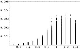
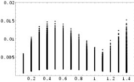
Figure 13: Predicted values of $|m_{\nu_{1}}|$ versus $h$ and $|m_{\nu_{2}}|$ versus $h$ in class $S_{1}$.

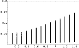
Figure 14: Predicted values of $|m_{\nu_{3}}|$ versus $h$ in class $S_{1}$.

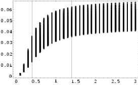
Figure 15: Predicted values of $|U_{e3}|$ versus $h$ in class $S_{1}$.

We can predict the values of $|U_{e3}|$,

$$|U_{e3}|\sim 0.01-0.06.$$ (4.32)

from Fig. 15. This value is not so large compared with the contribution from the charged lepton part, which is of order of $\lambda|U_{\mu 3}|\sim 0.01$, so the above prediction would yield additional ambiguity of $\sim 0.01$. We hope this can be checked by experiment in near future JHF-Kamioka long-base line [24], the sensitivity of which is reported as $|U_{e3}|\simeq 0.04$ at $90\%$ C.L. If we further expect Hyper-Kamiokande ($|U_{e3}|<10^{-2}$) [25], we can completely check whether such symmetric texture model can survive or not.

In conclusion we list a set of typical values of neutrino masses and mixings at $m_{t}\simeq 240~{}{\rm GeV}$:

$$\sin^{2}2\theta_{23} \sim 0.95-1,$$ (4.33)

$$\tan^{2}\theta_{12} \sim 0.23-0.6,$$ (4.34)

$$|U_{e3}| \sim 0.037-0.038,$$ (4.35)

$$|m_{\nu_{3}}| \sim 0.06-0.07~{}\rm eV,$$ (4.36)

$$|m_{\nu_{2}}| \sim 0.003-0.006~{}\rm eV,$$ (4.37)

$$|m_{\nu_{1}}| \sim 0.0007-0.0015~{}\rm eV,$$ (4.38)

with $m_{R}=2\times 10^{15}~{}{\rm GeV}$ and $rm_{R}=10^{8}~{}{\rm GeV}$, which corresponds to the Majorana mass for the third generation and those of the second and first generations, respectively.

Remark that, once the scale of right-handed Majorana mass matrix, $r$, is determined so as for the mixing angle of atmospheric neutrinos to become maximal, the same value $r$ well reproduces the large mixing angle of solar neutrinos and the two mass differences $\Delta m^{2}_{32}$ and $\Delta m^{2}_{21}$ with $m_{R}$. If we have more exact information of the experimental values, we need to include the CP phase factors in order to make more precise predictions, which is our next task.

5 Further Discussions

In general there are four cases as to the origin of large mixing for each mixing angle, $\theta_{23}$ and $\theta_{12}$. This can be summarized as follows:

1. Down Road Option: This is first proposed by Yanagida at the Takayama conference as a proper realization of non-parallel family structure and may be mostly regarded as a natural solution. Many proposals have been made to realize such non-parallel family structure [26, 27, 28]. It is indeed successful as to explain a large mixing angle, $\theta_{23}$ naturally. In this option we take non-symmetric down-type mass matrix under the observation that ${\bf 5^{*}}$ multiplets in $SU(5)$ GUT contains $SU(2)_{L}$ singlet down-quarks and doublet charged leptons. An example is the following non-symmetric mass matrix [29]

   $$M_{l}=M_{d}^{\rm T}\sim\left(\begin{array}[]{@{\,}ccc@{\,}}\epsilon^{2}&\epsilon^{2}&\epsilon^{2}\\ \epsilon&\epsilon&\epsilon\\ 1&1&1\end{array}\right).$$ (5.4)

   With a small number $\epsilon$ we can provide a large lepton mixing on the one hand, and a small down-quark mixing on the other hand. The remarkable fact implies that the mass matrix in the down-type sector is not symmetric even in such a large unification group as $E_{6}$ and that it leads to quite different lepton and down quark mixing angles. This is really realized even if we take such GUT larger than $E_{6}$, for example, by using E-twisted family structure [30].

2. Down-Up Option: However even if we can naturally reproduce large mixing angle of $\theta_{23}$, we need further tuning to get large mixing angle for $\theta_{12}$. This is really serious because most of the calculations are done only within “order of magnitude” arguments. Because of this, it is very difficult to get exact numbers of small parameters of the first and second generations. So there might be another possible option in which charged lepton mass matrix reproduces only large 2-3 mixing angle, leaving the neutrino mass matrix being responsible to derive solar large mixing angle.

3. Up-Down Option: This is the option in which $\sin^{2}2\theta_{23}$ is due to neutrino mass matrix and large $\tan^{2}\theta_{12}$ comes from charged lepton sector. However if it is so we can write

   $$V_{MNS} = U_{l}^{\dagger}U_{\nu}\simeq\left(\begin{array}[]{@{\,}ccc@{\,}}\cos\theta_{12}&\sin\theta_{12}&0\\ -\sin\theta_{12}&\cos\theta_{12}&0\\ 0&0&1\end{array}\right)\left(\begin{array}[]{@{\,}ccc@{\,}}1&0&0\\ 0&\cos\theta_{23}&-\sin\theta_{23}\\ 0&\sin\theta_{23}&\cos\theta_{23}\end{array}\right)$$ (5.11)

   $$= \left(\begin{array}[]{@{\,}ccc@{\,}}\cos\theta_{12}&\sin\theta_{12}\cos\theta_{23}&-\sin\theta_{12}\sin\theta_{23}\\ -\sin\theta_{12}&\cos\theta_{12}\cos\theta_{23}&-\cos\theta_{12}\sin\theta_{23}\\ 0&\sin\theta_{23}&\cos\theta_{23}\end{array}\right)$$ (5.15)

   which automatically induces large $|U_{e3}|$. This is already excluded by the CHOOZ experiment [31]: $|U_{e3}|<0.2$.

4. Up-Road Option: Both large mixing angles may come from neutrino sector. Even within $SU(5)$, the up-quark mass matrix is expressed in terms of ${\bf 10}\times{\bf 10}$, and simple symmetric texture is usually adopted. Then the Dirac neutrino mass matrix is also hierarchical with small mixing angles. A simple texture has been proposed for the right-handed Majorana neutrino mass matrix to give a large $\nu_{\tau}$-$\nu_{\mu}$ mixing [21]. Thus it is quite nontrivial question whether we can reproduce two large mixing angles if one concentrates on most economical symmetric texture.

We have investigated and checked all the types of textures for neutrino mass matrix, and fully investigated to confirm that the type $S_{1}$ is most proper one. As for the down-type Yukawa couplings we can compare the down quark with charged lepton masses and a good type has long been well known named Georgi-Jarlskog type mass matrix. On the other hand, until neutrino oscillation data were reported, we have had no information as to which representation of Higgs fields are relevant to up-type Yukawa couplings. Now that a good option for the Higgs configuration with symmetric 4-zero texture has been found, our next task would be to seek for the origin of the texture, which may be related to further higher symmetry or to the spatial structure including extra dimensions. We saw that the texture zero structure is very important to reproduce large mixing angles of neutrino mass matrix out of very small quark mass matrix. Such zero texture may be a reflection of family symmetry.

Note that our scenario is quite different from the down road option in which two large mixing angles observed in neutrino oscillation data come from the charged lepton side. One can predict some relations of neutrino mixing angles in terms of down quark information [32], for example. However even in such situation we can no more predict the absolute values of neutrino masses, which indeed needs the information of $M_{\nu}$. In the up road option, on the other hand, a remarkable fact is that we can predict all the neutrino (absolute) masses and mixing angles without any ambiguity. Our scenario, if it is indeed true, can be checked without any ambiguity even for the order-one coefficients. The remarkable results are obtained really thanks to the power of GUT. Our remaining task is to investigate the full mass matrix including CP phase. The GUT relation may simplify our analysis.

References

- [1] KamLAND Collaboration, K. Eguchi et al., Phys. Rev. Lett. 90 (2003) 021802.
- [2] M. Maltoni, T. Schwetz and J.W.F. Valle, arXiv: hep-ph/0212129.
- [3] G.L. Fogli et al., arXiv: hep-ph/0212127.
- [4] J.N. Bahcall, M.C. Gonzalez-Garcia, and C. Pena-Garay, arXiv: hep-ph/0212147.
- [5] P.C.de Holanda and A. Smirnov, arXiv: hep-ph/0212270.
- [6] Super-Kamiokande Collaboration, S. Fukuda et al., Phys. Lett. B433 (1998) 9; ibid. 436, 33 (1998); ibid. 539, 179 (2002).
- [7] Super-Kamiokande Collaboration, S. Fukuda et al., Phys. Rev. Lett. 86 (2001) 5651; ibid. 86, 5656 (2001).
- [8] SNO Collaboration, Q.R. Ahmad et al., Phys. Rev. Lett. 89 (2002) 011301; ibid. 89, 011302 (2002).
- [9] M.B. Smy [Super-Kamiokande Collaboration], arXiv: hep-ex/0206016.
- [10] M.C. Gonzalez-Garcia and Y. Nir, arXiv: hep-ph/0202058.
- [11] Z. Maki, M. Nakagawa and S. Sakata, Prog. Theor. Phys. 28 (1962) 870.
-
[12]
D. Du and Z.Z. Xing, Phys. Rev. D48 (1993) 2349;
H. Fritzsch and Z.Z. Xing, Phys. Lett. B353 (1995) 114;
K. Kang and S.K. Kang, Phys. Rev. D56 (1997) 1511;
J.L. Chkareuli and C.D. Froggatt, Phys. Lett. B450 (1999) 158. -
[13]
P.S. Gill and M. Gupta, Phys. Rev. D57 (1998) 3971;
M. Randhawa, V. Bhatnagar, P.S. Gill and M. Gupta, Phys. Rev. D60 (1999) 051301;
S.K. Kang and C.S. Kim, Phys. Rev. D63 (2001) 113010;
M. Randhawa, G. Ahuja and M. Gupta, arXiv: hep-ph/0230109. - [14] H. Georgi and C. Jarlskog, Phys. Lett. B86 (1979) 297.
- [15] P. Ramond, R.G. Roberts and G.G. Ross, Nucl. Phys. B406 (1993) 19.
- [16] S. Dimopoulos, L.J. Hall and S. Raby, Phys. Rev. Lett. 68 (1992) 1984; Phys. Rev. D45 (1992) 4195.
- [17] Y. Achiman and T. Greiner, Nucl. Phys. B443 (1995) 3.
- [18] J. Harvey, P. Ramond and D. Reiss, Phys. Lett. B92 (1980) 309; Nucl. Phys. B199 (1982) 223.
- [19] H. Nishiura, K. Matsuda and T. Fukuyama, Phys. Rev. D60 (1999) 013006. K. Matsuda, T. Fukuyama and H. Nishiura, Phys. Rev. D61 (2000) 053001.
- [20] C. D. Frogatt and H. B. Nielsen, Nucl. Phys. B147 (1979) 277.
- [21] M. Bando, T. Kugo and K. Yoshioka, Phys. Rev. Lett. 80 (1998) 3004.
- [22] H. Fusaoka and Y. Koide, Phys. Rev. D57 (1998) 3986.
- [23] M. Bando and M. Obara, arXiv: hep-ph/0212242.
- [24] Y. Itow et al., arXiv: hep-ex/0106019.
- [25] M. Aoki, K. Hagiwara, Y. Hayayo, T. Kobayashi, T Nakaya, K. Nishikawa and N. Okamura, arXiv: hep-ph/0112338.
- [26] T. Yanagida, Talk given at 18th International Conference on Neutrino Physics and Astrophysics (NEUTRINO 98), Takayama, Japan, 4-9 Jun 1998; arXiv: hep-ph/9809307.
- [27] J. Sato and T. Yanagida, Phys. Lett. B430 (1998) 127.
- [28] Y. Nomura and T. Yanagida, Phys. Rev. D59 (1998) 017303.
- [29] H. Haba and H. Murayama, Phys. Rev. D63 (2001) 053010
- [30] M. Bando and T. Kugo, Prog. Theor. Phys. 101 (1999) 1313.
- [31] M. Apollonio et al. (CHOOZ Collaboration), Phys. Lett. B420 (1998) 397.
- [32] M. Bando, T. Kugo and K. Yoshioka, Phys. Lett. B483 (2000) 163.