NSF-KITP-03-12

Probing the neutrino mass hierarchy and the 13-mixing with supernovae

Cecilia Lunardini^a,b,1 and Alexei Yu. Smirnov^c,d,2

^a Institute for Advanced Study, Einstein drive, 08540 Princeton, New Jersey, USA

^bKavli Institute for Theoretical Physics, University of California Santa Barbara, California, 93106-4030, USA

^c The Abdus Salam ICTP, Strada Costiera 11, 34100 Trieste, Italy

^d Institute for Nuclear Research, RAS, Moscow 123182, Russia.

We consider in details the effects of the 13-mixing ($\sin^{2}\theta_{13}$) and of the type of mass hierarchy/ordering (sign[$\Delta m^{2}_{13}$]) on neutrino signals from the gravitational collapses of stars. The observables (characteristics of the energy spectra of $\nu_{e}$ and $\bar{\nu}_{e}$ events) sensitive to $\sin^{2}\theta_{13}$ and sign[$\Delta m^{2}_{13}$] have been calculated. They include the ratio of average energies of the spectra, $r_{E}\equiv\langle E\rangle/\langle\bar{E}\rangle$, the ratio of widths of the energy distributions, $r_{\Gamma}\equiv\Gamma/\bar{\Gamma}$, the ratios of total numbers of $\nu_{e}$ and $\bar{\nu}_{e}$ events at low energies, $S$, and in the high energy tails, $R_{tail}$. We construct and analyze scatter plots which show the predictions for the observables for different intervals of $\sin^{2}\theta_{13}$ and signs of $\Delta m^{2}_{13}$, taking into account uncertainties in the original neutrino spectra, the star density profile, etc.. Regions in the space of observables $r_{E}$, $r_{\Gamma}$, $S$, $R_{tail}$ exist in which certain mass hierarchy and intervals of $\sin^{2}\theta_{13}$ can be identified or discriminated. We elaborate on the method of the high energy tails in the spectra of events. The conditions are formulated for which $\sin^{2}\theta_{13}$ can be (i) measured, (ii) restricted from below, (iii) restricted from above. We comment on the possibility to determine $\sin^{2}\theta_{13}$ using the time dependence of the signals due to the propagation of the shock wave through the resonance layers of the star. We show that the appearance of the delayed Earth matter effect in one of the channels ($\nu_{e}$ or $\bar{\nu}_{e}$) in combination with the undelayed effect in the other channel will allow to identify the shock wave appeareance and determine the mass hierarchy.

PACS: 14.60.Pq, 97.60.Bw.

Keywords: neutrino conversion; matter effects; supernova.

¹ E-mail: lunardi@ias.edu ² E-mail: smirnov@ictp.trieste.it

1 Introduction

Collapsing stars (some of them appearing as supernova explosions) are the sources of neutrinos of different flavors which can be used for oscillation/conversion experiments [1]. The structure of the neutrino mass spectrum and lepton mixing is imprinted into the detected signal (see [2]–[13] as an incomplete list of relevant works). Therefore, in principle, studying the properties of a supernova neutrino burst one can get information about

• the values of parameters relevant for the solution of the solar neutrino problem,

• the type of the mass hierarchy/ordering,

• the 13-mixing parameter $\sin^{2}\theta_{13}$,

• the presence of sterile neutrinos,

• new neutrino interactions.

The first KamLAND results [14] confirmed the LMA MSW as the dominant mechanism of the solar neutrino conversion. Further KamLAND measurements and solar neutrino studies will determine the corresponding oscillation parameters with rather good accuracy  [15, 16, 17]. This confirmation implies, in particular, that already in 1987, with the detection of neutrinos from the supernova SN1987A, significant conversion effects were observed on supernova neutrinos [18]–[26]. The identification of the neutrino mass hierarchy and the determination of 13-mixing ($\sin^{2}\theta_{13}$) have become the main issues of further studies. Searches for sterile neutrinos and new neutrino interactions are also on the agenda.

In this paper we will concentrate on the related subjects of the mass hierarchy and $\sin^{2}\theta_{13}$. We will consider a three neutrinos system, assuming that sterile neutrinos, if they exist, produce negligible effect.

The possibilities to study neutrino conversion effects using supernovae are wide, but not exempt of problems. The main difficulty originates from the fact that oscillation effects are proportional to the difference of the electron and non-electron neutrino fluxes originally produced inside the star, which are poorly known at the moment. The features of these fluxes depend on many details of the neutrino transport inside the star and, in general, on the type of progenitor star.

There are two approaches to resolve the problem:

1). perform a global fit of the data, determining both oscillation parameters and the parameters of the original fluxes simultaneously. However, the number of unknown parameters which describe the energy spectra of the emitted neutrinos (temperatures, luminosities, pinching parameters) is rather large, and moreover, these quantities change with time during the burst.

Also degeneracies of parameters exist, so that variations of the oscillation parameters and of the parameters of the fluxes can produce the same observable effect.

2). perform a (supernova) model independent analysis relying on some generic (and model independent) qualitative features of the fluxes. Namely:

- the inequality of average energies (temperatures) of the original fluxes of neutrinos of different flavors;

- the dominance of the electron neutrino flux in the initial phase of the burst (neutronization peak)

- the pinching of the energy spectra

- the approximate equality of the original $\nu_{\mu}$, $\bar{\nu}_{\mu}$, $\nu_{\tau}$, $\bar{\nu}_{\tau}$ fluxes.

The first approach has been used recently in [10, 11], while the study of ratios of numbers of events in specific energy intervals has been suggested in [8, 13].

In this paper we elaborate the second type of approach, suggesting specific methods and taking into account all the possible uncertainties. Both analytical and numerical analyses are performed. The paper is organized as follows. In sect. 2 we summarize our knowledge of the original neutrino spectra and of the matter distribution along the trajectory of the neutrinos in the star. We also introduce the scheme of neutrino masses and mixings. In sect. 3. the dependence of the conversion probabilities of supernova neutrinos on the mass hierarchy and the 13-mixing is considered. In sect. 4 we introduce observables which are sensitive to $\sin^{2}\theta_{13}$ and sign[$\Delta m^{2}_{13}$]. In sect. 5 we calculate these observables for normal and inverted hierarchy and different intervals of $\sin^{2}\theta_{13}$, identifying the regions in the space of these observables in which the mass hierarchy and $\sin^{2}\theta_{13}$ can be determined. In sect. 6 we elaborate on the method of the high energy tails of the spectra produced in the detectors by neutrinos and antineutrinos. Sec. 7 is devoted to the study of the possibility to restrict $\sin^{2}\theta_{13}$ using the time variations of signals induced by the shock wave propagation. Conclusions are given in sect. 8.

2 Fluxes, density profile, neutrino mass spectrum

2.1 Properties of supernova neutrino fluxes

In this section we summarize our present knowledge of the neutrino fluxes from the collapsing stars.

At a given time $t$ from the core collapse the original flux of the neutrinos of a given flavor, $\nu_{\alpha}$, can be described by a “pinched” Fermi-Dirac (F-D) spectrum,

$$F^{0}_{\alpha}(E,T_{\alpha},\eta_{\alpha},L_{\alpha},D)=\frac{L_{\alpha}}{4\pi D^{2}T^{4}_{\alpha}F_{3}(\eta_{\alpha})}\frac{E^{2}}{e^{E/T_{\alpha}-\eta_{\alpha}}+1}~{},$$ (1)

where $D$ is the distance to the supernova (typically $D\sim 10$ kpc for a galactic supernova), $E$ is the energy of the neutrinos, $L_{\alpha}$ is the luminosity of the flavor $\nu_{\alpha}$, and $T_{\alpha}$ represents the effective temperature of the $\nu_{\alpha}$ gas inside the neutrinosphere. Supernova simulations provide the indicative values of the average energies [27]:

$$\langle E_{\bar{e}}\rangle=(14-22)~{}{\rm MeV},~{}~{}~{}\langle E_{x}\rangle/\langle E_{\bar{e}}\rangle=(1.1-1.6),~{}~{}~{}\langle E_{e}\rangle/\langle E_{\bar{e}}\rangle=(0.5-0.8),~{}~{}~{}$$ (2)

and the typical value of the (time-integrated) luminosity in each flavor: $L_{\alpha}\sim(1-5)\cdot 10^{52}~{}{\rm ergs}$. The intervals in eq. (2) include the results of recent Monte-Carlo simulations [27], in which a difference between $\langle E_{x}\rangle$ and $\langle E_{\bar{e}}\rangle$ of about $10\%$ is given as typical, though differences as small as few per cent are not excluded. We will briefly comment on this latter case in the discussion of our results. The $\mathrel{{\nu_{\mu}}}$ and $\mathrel{{\nu_{\tau}}}$ ($\mathrel{{\bar{\nu}}_{\mu}}$ and $\mathrel{{\bar{\nu}}_{\tau}}$) spectra are equal with good approximation, and therefore the two species can be treated as a single one, $\mathrel{{\nu_{x}}}$ ($\mathrel{{\bar{\nu}}_{x}}$). Conversely, small differences exist between the energy spectra of the non-electron neutrinos and antineutrinos, $\mathrel{{\nu_{x}}}$ and $\mathrel{{\bar{\nu}}_{x}}$, due to effects of weak magnetism, [28]. In particular, the difference

$$\delta_{x}\equiv T_{\bar{x}}-T_{x}=0.4-0.5~{}~{}{\rm MeV}$$ (3)

is found to be valid with $\sim 20\%$ accuracy over a large variety of physical situations [28]. The luminosities of all neutrino species are expected to be approximately equal, within a factor of two or so [1, 30]:

$${L_{e}}/{L_{x}}=(0.5-2),~{}~{}~{}L_{\bar{e}}/L_{\bar{x}}=(0.5-2),~{}~{}~{}L_{\bar{x}}\simeq L_{x}.$$ (4)

The pinching parameter $\eta_{\alpha}$ takes the values

$$\eta_{e}\sim 0-3,~{}~{}~{}~{}\eta_{\bar{e}}\sim 0-3~{}~{}~{}~{}\eta_{\mu}=\eta_{\tau}\sim 0-2.$$ (5)

Notice that the $\nu_{e}$ and $\mathrel{{\bar{\nu}}_{e}}$ spectra may have stronger pinching than the other flavors [29, 30].

In eq. (1) the normalization factor $F_{3}(\eta_{\alpha})$ equals:

$$F_{3}(\eta_{\alpha})\equiv\int_{0}^{\infty}\frac{x^{3}}{e^{x-\eta_{\alpha}}+1}dx~{}.$$ (6)

In the absence of pinching, $\eta_{\alpha}=0$, one gets $F_{3}(0)=7\pi^{4}/120\simeq 5.68$. The average energy $\langle E_{\alpha}\rangle$ of the spectrum depends on both $T_{\alpha}$ and $\eta_{\alpha}$; for $\eta_{\alpha}=0$ we have $\langle E_{\alpha}\rangle\simeq 3.15~{}T_{\alpha}$.

The luminosity, temperature and pinching of the neutrino flux vary with the time $t$; Time dependence can be different for different stars [27]. If these variations occur over time scales larger than the duration of the burst, $\tau\sim 10$ s, the integrated $\nu_{\alpha}$ flux is can be described by the expression (1) but with smaller $\eta_{\alpha}$ (integration leads to widening of spectra).

2.2 Matter profile

In our study of neutrino conversions inside the star we use the following matter density profile of the star:

$$\rho(r)=10^{13}~{}C\left(\frac{10~{}{\rm km}}{r}\right)^{3}~{}{\rm g\cdot cm^{-3}}~{},$$ (7)

with $C\simeq 1-15$ [31, 20, 32, 29]. For $\rho\sim(1-10^{5})~{}{\rm g\cdot cm^{-3}}$ expression (7) provides a good approximation to the calculated matter distribution during at least the first few seconds of the neutrino burst emission. For $\rho\mathrel{\vbox{\hbox{$<$}\nointerlineskip\hbox{$\sim$}}}1~{}{\rm g\cdot cm^{-3}}$ the exact shape of the profile depends on the details of evolution of the star, its chemical composition, rotation, etc.. As it was recently pointed out [33], after $\sim(2-10)$ seconds from the core collapse and bounce, the shock-wave propagating inside the star could reach the regions relevant to neutrino resonant conversion and modify the observed neutrino signal.

For three active neutrinos the difference of the $\mathrel{{\nu_{e}}}$ and $\mathrel{{\nu_{x}}}$ potentials in matter depends on the number density of electrons: $n_{e}=Y_{e}\rho/m_{N}$, where $m_{N}$ is the nucleon mass and $Y_{e}$ is the number of electrons per nucleon. The transitions occur mainly in the isotopically neutral region where $Y_{e}=1/2$ with rather good precision.

2.3 Neutrino mixing and mass spectra

We study the effects of neutrino flavor conversion in the star and in the Earth in a three neutrino framework with mixing and mass splittings allowed by the atmospheric and solar neutrino data.

The neutrino mass eigenstates, $\nu_{i}$ ($i=1,2,3$), with masses $m_{i}$ are related to the flavor eigenstates, $\nu_{\alpha}$ ($\alpha=e,\mu,\tau$), by the mixing matrix $U$: $\nu_{\alpha}=\sum_{i}U_{\alpha i}\nu_{i}$. The standard parameterization of this matrix is used here (see e.g. [34]). The atmospheric neutrino data determine [35]:

$$m_{3}^{2}-m_{2}^{2}\equiv\Delta m^{2}_{32}=\pm(1.5-4)\cdot 10^{-3}{\rm eV}^{2},~{}~{}~{}~{}~{}~{}~{}\tan^{2}\theta_{23}=0.48-2.1~{}.$$ (8)

The two possibilities, $\Delta m^{2}_{32}\approx\Delta m^{2}_{31}>0$ and $\Delta m^{2}_{32}\approx\Delta m^{2}_{31}<0$, are referred to as normal and inverted mass hierarchies/ordering respectively and will be denoted as n.h. and i.h. in the text.

The solar neutrino data and the KamLAND results select the large mixing angle (LMA) MSW solution with parameters (see e.g. [14], [36]–[39]):

$$m_{2}^{2}-m_{1}^{2}\equiv\Delta m^{2}_{21}=(4-30)\cdot 10^{-5}{\rm eV}^{2},~{}~{}~{}~{}~{}~{}\tan^{2}\theta_{12}=0.25-0.85~{}.$$ (9)

The reactor experiments CHOOZ and Palo Verde give the upper bound on 13-mixing [40, 41]:

$$\sin^{2}\theta_{13}\mathrel{\vbox{\hbox{$<$}\nointerlineskip\hbox{$\sim$}}}0.02~{}.$$ (10)

3 Mass hierarchy, $U_{e3}$ and conversion effects

3.1 Permutation factors

The fluxes $F_{e}$ and $F_{\bar{e}}$ of the electron neutrinos and antineutrinos in the detector can be expressed in terms of the permutation parameters $(1-p)$ and $(1-\bar{p})$ and the original fluxes as follows [5]:

$$F_{e}={p}F_{e}^{0}+(1-{p})F_{x}^{0}=F_{e}^{0}+(1-p)(F_{x}^{0}-F_{e}^{0})~{}~{},$$ (11)

$$F_{\bar{e}}={\bar{p}}F_{\bar{e}}^{0}+(1-{\bar{p}})F_{\bar{x}}^{0}=F_{\bar{e}}^{0}+(1-{\bar{p}})(F_{\bar{x}}^{0}-F_{\bar{e}}^{0})~{}.$$ (12)

The factors $p$ and ${\bar{p}}$ are the total $\nu_{e}$ and $\bar{\nu}_{e}$ survival probabilities which describe the conversion effects inside the star, in the intergalactic medium, and, if the Earth is crossed, in the matter of the Earth. As can be seen in eqs. (11, 12), the conversion effects are proportional to the difference of the original $\mathrel{{\nu_{e}}}$ ($\mathrel{{\bar{\nu}}_{e}}$) and $\mathrel{{\nu_{x}}}$ ($\mathrel{{\bar{\nu}}_{x}}$) fluxes.

As they propagate in the star, the neutrinos undergo two MSW resonances (level crossings):

(i) the first resonance (H) occurs at higher density, $\rho\sim 10^{3}~{}{\rm g\cdot cm^{-3}}(10{\rm MeV}/E)$, it is governed by the atmospheric mass squared splitting, $\Delta m^{2}_{32}$, and by the $\theta_{13}$ angle. The H-resonance is in the neutrino (antineutrino) channel if the mass hierarchy is normal (inverted). The probability of transition between the eigenstates of the Hamiltonian (jumping probability) in this resonance, $P_{H}$, can be written for the density profile (7) as [5]:

$$P_{H}=\exp\left[-\left(\frac{E_{na}}{E}\right)^{2/3}\right]~{},$$ (13)

$$E_{na}\simeq 1.08\cdot 10^{7}~{}{\rm MeV}\left(\frac{|\Delta m^{2}_{32}|}{10^{-3}~{}{\rm eV}^{2}}\right)C^{1/2}\sin^{3}\theta_{13}~{}.$$ (14)

The probability $P_{H}$ has been obtained on the basis of the Landau-Zener (LZ) formula which holds for the linear density distribution. It can be checked that for small mixing (as it is the case here) the formula works well for the density profile (7) [42, 43, 9].

(ii) A second level crossing (L) determined by the “solar” parameters (9), happens at lower density, $\rho\sim(30-140)(10{\rm MeV}/E)~{}{\rm g\cdot cm^{-3}}$. For $\Delta m^{2}_{21}$ and $\theta_{12}$ in the LMA region the propagation through this resonance is adiabatic for all possible values of $C$ [5].

Let us first consider the effects of conversion in the star with no Earth crossing. We will use here the approximation of “factorized dynamics” in the resonances, which means that the dynamics of level crossing in the two resonances are independent and the total survival probability is the product of the survival probabilities in each resonance (see [5] for details). In this approximation the survival probabilities $p$ and ${\bar{p}}$ equal [5]:

$$p\simeq P_{H}|U_{e2}|^{2}+(1-P_{H})|U_{e3}|^{2},$$ (15)

$${\bar{p}}\simeq~{}|U_{e1}|^{2},$$ (16)

for n.h. and

$$p\simeq|U_{e2}|^{2}$$ (17)

$${\bar{p}}\simeq P_{H}|U_{e1}|^{2}+(1-P_{H})|U_{e3}|^{2}$$ (18)

for i.h.. The transition from normal to inverted hierarchy cases corresponds to the interchange of the permutation factors, $p\leftrightarrow\bar{p}$, and of the indices $1\leftrightarrow 2$ in the mixing parameters.

Using the standard parameterization of the mixing matrix, according to which

$$|U_{e1}|^{2}=\cos^{2}\theta_{12}\cos^{2}\theta_{13},~{}~{}~{}|U_{e2}|^{2}=\sin^{2}\theta_{12}\cos^{2}\theta_{13},~{}~{}~{}|U_{e3}|^{2}=\sin^{2}\theta_{13},$$ (19)

we can rewrite the survival probabilities in the following form

$$p\simeq P_{H}\sin^{2}\theta_{12}~{}+\left[1-P_{H}(1+\sin^{2}\theta_{12})\right]\sin^{2}\theta_{13}~{},$$ (20)

$${\bar{p}}\simeq\cos^{2}\theta_{12}(1-\sin^{2}\theta_{13})~{},$$ (21)

for n.h. and

$$p\simeq\sin^{2}\theta_{12}(1-\sin^{2}\theta_{13})~{},$$ (22)

$${\bar{p}}\simeq P_{H}\cos^{2}\theta_{12}+\left[1-P_{H}(1+\cos^{2}\theta_{12})\right]\sin^{2}\theta_{13}~{},$$ (23)

for i.h..

The permutation factors depend on $\sin^{2}\theta_{13}$ via the jumping probability $P_{H}\equiv P_{H}(\sin^{2}\theta_{13})$ and explicitly via the mixing parameters. A further dependence of the permutation factors on $\theta_{13}$ is given by small terms which are neglected in our approximation. They arise from:

1) generalizing the LZ expression for $P_{H}$: a more precise double exponential form of the jumping probability $P_{H}$ (see e.g. [44]) gives $\sin^{2}\theta_{13}$ corrections to the Landau-Zener form. These corrections appear however with very small coefficients and therefore can be neglected.

2) relaxing the approximation of factorized dynamics: this could give linear (in $\sin\theta_{13}$) corrections of the form $\sin\theta_{13}\Delta m^{2}_{21}/\Delta m^{2}_{31}$. For the large $\Delta m^{2}_{21}$ part of the LMA region we have $|\Delta m^{2}_{21}/\Delta m^{2}_{31}|\sim 0.1$, which is large enough so that $\sin\theta_{13}|\Delta m^{2}_{21}/\Delta m^{2}_{31}|\sim\sin^{2}\theta_{13}$ and the linear terms can not be neglected with respect to the $\mathrel{{\sin^{2}\theta_{13}}}$ ones. In contrast, taking the best fit values of the mass squared splittings one gets $|\Delta m^{2}_{21}/\Delta m^{2}_{31}|\sim 10^{-2}$, therefore the $\mathrel{{\sin^{2}\theta_{13}}}$ terms dominate for $\mathrel{{\sin^{2}\theta_{13}}}\mathrel{\vbox{\hbox{$>$}\nointerlineskip\hbox{$\sim$}}}10^{-3}$. A detailed study of the deviation from the factorization will be given elsewhere [45].

Two limits are important:

1). If $\theta_{13}$ is very small so that $P_{H}=1$, both mass hierarchies lead to the same result:

$$p\simeq\sin^{2}\theta_{12},~{}~{}~{}{\bar{p}}\simeq\cos^{2}\theta_{12}~{}.$$ (24)

2). For large enough $\theta_{13}$ (in practice for $\mathrel{{\sin^{2}\theta_{13}}}\mathrel{\vbox{\hbox{$>$}\nointerlineskip\hbox{$\sim$}}}10^{-3}$ see the next subsection) when $P_{H}=0$ we have

$$p\simeq\sin^{2}\theta_{13}~{},~{}~{}~{}~{}{\bar{p}}\simeq\cos^{2}\theta_{12}(1-\sin^{2}\theta_{13})\approx\cos^{2}\theta_{12}~{}~{}~{}~{}~{}~{}~{}{\rm~{}~{}(n.h.)}~{},$$ (25)

and

$$p\simeq\sin^{2}\theta_{12}(1-\sin^{2}\theta_{13})\approx\sin^{2}\theta_{12}~{},~{}~{}~{}{\bar{p}}\simeq\sin^{2}\theta_{13}~{}~{}~{}~{}~{}~{}~{}{\rm~{}~{}(i.h.)}~{}.$$ (26)

Let us underline that in this limit uncertainties related to the density profile or with factorized dynamics disappear. The conversion is strongly adiabatic and the results (25, 26) are exact. Notice also that from the point of view of present oscillation results (large or maximal 12 and 23 mixings) such a possibility looks rather plausible.

3.2 $P_{H}$ and $\sin^{2}\theta_{13}$

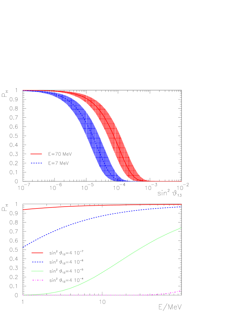
Figure 1: The transition probability in the H resonance, $P_{H}$, as a function of $\mathrel{{\sin^{2}\theta_{13}}}$ for two values of the neutrino energy (upper panel) and of the neutrino energy for different values of $\mathrel{{\sin^{2}\theta_{13}}}$ (lower panel). We took $C=4$ and $|\Delta m^{2}_{32}|=3\cdot 10^{-3}~{}{\rm eV^{2}}$. The shaded regions in the upper panel represent the uncertainty associated to $C=1-15$.

The jumping probability $P_{H}$ is shown in fig. 1 (upper panel, central lines) as a function of $\mathrel{{\sin^{2}\theta_{13}}}$ for two extreme neutrino energies and the parameters $|\Delta m^{2}_{32}|=3\cdot 10^{-3}{\rm eV^{2}}$ and $C=4$. As follows from eq. (13), a constant value of $P_{H}$ corresponds to $\sin^{2}\theta_{13}\propto E^{2/3}$. This determines the shift of the curve $P_{H}$ in Fig. 1 along the axis $\sin^{2}\theta_{13}$ with change of energy.

From the figure it follows that, for all neutrino energies relevant for observations, the conversion in the H resonance is adiabatic ($P_{H}=0$) for $\mathrel{{\sin^{2}\theta_{13}}}\mathrel{\vbox{\hbox{$>$}\nointerlineskip\hbox{$\sim$}}}4\cdot 10^{-4}$. The adiabaticity is maximally violated ($P_{H}=1$) for $\mathrel{{\sin^{2}\theta_{13}}}\mathrel{\vbox{\hbox{$<$}\nointerlineskip\hbox{$\sim$}}}4\cdot 10^{-6}$. In the intermediate region $P_{H}$ depends significantly on $\mathrel{{\sin^{2}\theta_{13}}}$, decreasing from 1 to 0 as $\mathrel{{\sin^{2}\theta_{13}}}$ increases.

Let us consider the uncertainties in the relation between $P_{H}$ and $\sin^{2}\theta_{13}$. The uncertainty in $P_{H}$ due to a variation of $C$ by factor (1/4 - 4) is shown in fig. 1 as a shadowed band. As given in eq. (13), a constant value of $P_{H}$ corresponds to $\sin^{2}\theta_{13}\propto C^{-1/3}$. Thus, for a given $P_{H}$, the variation of $C$ corresponds to a variation of $\sin^{2}\theta_{13}$ by factor 2.6.

Furthermore, the profile (7) is a simplification and deviations from cubic dependence can appear if [46]:

1. the energy transfer in the star is not purely radiative but also convective.

2. the luminosity $L$ is not constant with the radius $r$ [46].

3. the opacity $k$ has a spatial dependence: $k=k(r)$.

In general, one can fit a realistic profile which appears from numerical models of supernova progenitors by $\rho\propto r^{-n(r)}$. It can be seen that $n=3$ provides the best power law fit of the realistic profile, however local deviations can be significant with variations of index in the interval $n=1\div 5$ [9, 47].

As discussed in ref. [5], if the position of the resonance, $r_{res}$, is kept fixed, the adiabaticity parameter $\gamma$ scales as $n^{-1}$:

$$\gamma \equiv \frac{|\Delta m^{2}_{13}|}{2E}\frac{\sin^{2}2\theta_{13}}{\cos 2\theta_{13}}\frac{1}{|(dn/dr)/n|_{res}}\approx\frac{2|\Delta m^{2}_{13}|r_{res}}{E}\frac{\sin^{2}\theta_{13}}{n}~{}.$$ (27)

So, the uncertainty $n=1\div 5$ corresponds to a factor $\sim 2-3$ uncertainty in $\sin^{2}\theta_{13}$ with respect to the $n=3$ case.

Thus, the absolute limitation in determination of $\sin^{2}\theta_{13}$ from measurements of $P_{H}$, can be characterized by the factor 1/3 - 3, unless the knowledge of the star profile will be substantially improved. In principle, the uncertainty on the density profile can be reduced if the progenitor of the star is identified and detailed observations of the supernova optical signal (light curve, etc.) is done.

The uncertainty due to the error in $\Delta m^{2}_{31}$ is numerically less important. We take it to be of $\sim 20\%$, in agreement with the expected precision of near future measurements [48].

$P_{H}$ as a function of energy for different values of $\mathrel{{\sin^{2}\theta_{13}}}$ is given in the bottom panel of fig. 1. In the observable part of the spectrum, $E=(5-70)$ MeV, a strong dependence of $P_{H}$ on $E$, and consequently the strongest distortion of the energy spectrum, is expected if $\sin^{2}\theta_{13}=(1-5)\cdot 10^{-5}$. For $\sin^{2}\theta_{13}=4\cdot 10^{-5}$ the probability $P_{H}$ increases with $E$ by factor of 5 in the observable part of spectrum. Effects due to this strong change could give the possibility to probe $\theta_{13}$ is this region. The energy dependence is very weak for $\sin^{2}\theta_{13}>4\cdot 10^{-4}$ and $\sin^{2}\theta_{13}<4\cdot 10^{-6}$.

3.3 Three regions

According to eqs. (20)-(21) for the normal mass hierarchy, the probability in the antineutrino channel, $\bar{p}$, does not depend on the neutrino energy and only very weakly depends on $\theta_{13}$ via the $\mathrel{{\sin^{2}\theta_{13}}}$ term. In contrast, for the neutrino channel the permutation factor, $1-p$, depends on the energy via the $P_{H}$ parameter and on the $\theta_{13}$ angle both explicitly (the $\mathrel{{\sin^{2}\theta_{13}}}$ term in eq. (20)) and implicitly through $P_{H}$ (eq. (13)). This dependence is illustrated in the upper panel of fig. 2 for different values of the neutrino energy, $\mathrel{{\tan^{2}\theta_{12}}}=0.38$ and the other parameters as in fig. 1. According to the expression (20) and to the figure we can distinguish three regions:

(i) Adiabaticity breaking region:

$$\mathrel{{\sin^{2}\theta_{13}}}\mathrel{\vbox{\hbox{$<$}\nointerlineskip\hbox{$\sim$}}}10^{-6}\left(\frac{E}{10{\rm MeV}}\right)^{2/3}.$$ (28)

For these values of $\mathrel{{\sin^{2}\theta_{13}}}$ one gets $P_{H}\simeq 1$ and the first term in eq. (20) dominates. For $\mathrel{{\sin^{2}\theta_{13}}}\rightarrow 0$: $p\approx\sin^{2}\theta_{12}$ with very good approximation, independently of the values of $\mathrel{{\sin^{2}\theta_{13}}}$ and of the neutrino energy. In this region the conversion in the H resonance has little effect and the permutation is due to adiabatic conversion in the L-resonance.

(ii) Transition region:

$$\mathrel{{\sin^{2}\theta_{13}}}\sim(10^{-6}-10^{-4})\cdot\left(\frac{E}{10{\rm MeV}}\right)^{2/3}.$$ (29)

In this region $P_{H}$ takes intermediate values between 1 and 0 (see fig. 1). Still $\mathrel{{\sin^{2}\theta_{13}}}$ corrections to the permutation factor are negligible, so that $p\simeq P_{H}\sin^{2}\theta_{12}$; the permutation $(1-p)$ increases with $\mathrel{{\sin^{2}\theta_{13}}}$, following the jumping probability $P_{H}$.

(iii) Adiabatic region:

$$\mathrel{{\sin^{2}\theta_{13}}}\mathrel{\vbox{\hbox{$>$}\nointerlineskip\hbox{$\sim$}}}10^{-4}\left(\frac{E}{10{\rm MeV}}\right)^{2/3}.$$ (30)

Here $P_{H}\simeq 0$ and therefore the two terms in eq. (20) are comparable near the border of the region and with increase of $\mathrel{{\sin^{2}\theta_{13}}}$ the second term dominates. The survival probability $p$ has a minimum at $\mathrel{{\sin^{2}\theta_{13}}}\sim 10^{-3}$, corresponding to nearly maximal permutation. For $\mathrel{{\sin^{2}\theta_{13}}}\mathrel{\vbox{\hbox{$>$}\nointerlineskip\hbox{$\sim$}}}10^{-3}$ the term of order $\mathrel{{\sin^{2}\theta_{13}}}$ in the permutation factor starts to dominate and $p\simeq\mathrel{{\sin^{2}\theta_{13}}}$.

For inverted hierarchy similar results are found with the substitution $\nu\leftrightarrow\bar{\nu}$: $p$ has only a (small) explicit dependence on $\mathrel{{\sin^{2}\theta_{13}}}$, while $\bar{p}$ depends on $\mathrel{{\sin^{2}\theta_{13}}}$ both explicitly and implicitly (see eq. (23)). The same three regions discussed here can be identified according to the adiabaticity character of the H resonance. The explicit dependence of $\bar{p}$ on $\mathrel{{\sin^{2}\theta_{13}}}$ dominates for $\mathrel{{\sin^{2}\theta_{13}}}\mathrel{\vbox{\hbox{$>$}\nointerlineskip\hbox{$\sim$}}}10^{-3}$, where $\bar{p}\simeq\mathrel{{\sin^{2}\theta_{13}}}$. These features are shown in the lower panel of fig. 2.

The effects of the explicit dependence of $p$ (or $\bar{p}$) on $\mathrel{{\sin^{2}\theta_{13}}}$ in observable signals are smaller than $\sim 2\%$ and it will be very difficult to study them due to larger experimental and theoretical uncertainties. However, their identification may be within the reach of the next generation large volume detectors like HyperKamiokande [49], UNO [50, 51] and TITAND [52].

If the accuracy of the experiments is not better than a few % one can neglect the explicit dependence of the probabilities on $\theta_{13}$. In this case the permutation factor and therefore the observable effects depend on $\theta_{13}$ only via the jumping probability. So one can solve the problem in two steps:

- measure $P_{H}$ immediately from experiments

- use the relation between $P_{H}$ and $\theta_{13}$ to determine $\sin^{2}\theta_{13}$.

Summarizing, according to (11), (12) and (20) - (23) the effects of $\theta_{13}$ consist of

• change of the degree of permutation;

• distortion of the energy spectrum due to dependence of the jumping factor on energy.

For normal hierarchy a change of the neutrino permutation factor, $(1-p)$, is smaller than $30\%$: from $\cos^{2}\theta_{12}\approx 0.73$ at very small $\theta_{13}$ to $\approx 1$ at $\theta_{13}>10^{-3}$. The change of antineutrino factor is negligible. Notice that, for any value of $\theta_{13}$, the conversion inside the star leads to the composite spectrum and $\theta_{13}$ changes the level of this compositeness.

Thus, to determine $\theta_{13}$ in the case of normal hierarchy one needs to distinguish between completely permuted $\mathrel{{\nu_{e}}}$ spectrum, with $F_{e}\approx F_{x}^{0}$, and strongly (3/4 or more) permuted spectrum. In the first case one expects a signal which corresponds to the Fermi-Dirac spectrum, whereas in the second case, a composite spectrum appears with the dominant hard component.

Clearly, to get an information about $\theta_{13}$ one needs, in general, to know the original neutrino fluxes with better than $30\%$ accuracy (including also substantial uncertainties of the detection procedure).

For inverted mass hierarchy the change of the antineutrino permutation due to $\theta_{13}$ is more significant: $(1-\bar{p})$ increases from $\sin^{2}\theta_{12}\sim 0.27$ for very small $\theta_{13}$ to about 1 for $\theta_{13}>10^{-3}$. However, in this case the effect of permutation is suppressed due to smaller difference of the original $\mathrel{{\bar{\nu}}_{e}}$ and $\mathrel{{\bar{\nu}}_{x}}$ fluxes. The change of neutrino permutation is negligible.

The permutation of $\mathrel{{\nu_{e}}}$ and $\mathrel{{\nu_{x}}}$ (or $\mathrel{{\bar{\nu}}_{e}}$ and $\mathrel{{\bar{\nu}}_{x}}$) spectra, and therefore the observed neutrino signal, are mostly sensitive to $\mathrel{{\sin^{2}\theta_{13}}}$ in the transition region; any dependence on $\mathrel{{\sin^{2}\theta_{13}}}$ outside this interval is negligible. In other words,

• for $\mathrel{{\sin^{2}\theta_{13}}}>10^{-3}$ the effect of 1-3 mixing is strong in neutrino (antineutrino) channel if the mass hierarchy is normal (inverted). This makes it possible to determine the hierarchy of the neutrino mass spectrum, while it is difficult to measure $\mathrel{{\sin^{2}\theta_{13}}}$. Observations of corresponding conversion effects will allow to put a lower bound on $\mathrel{{\sin^{2}\theta_{13}}}$.

• in the region $\mathrel{{\sin^{2}\theta_{13}}}\sim(3\cdot 10^{-4}-3\cdot 10^{-6})$ measurements of $\mathrel{{\sin^{2}\theta_{13}}}$ are possible, or at least both upper and lower bounds on $\mathrel{{\sin^{2}\theta_{13}}}$ can be obtained; values of $\mathrel{{\sin^{2}\theta_{13}}}$ in this region are at least one order of magnitude below the sensitivity of planned terrestrial experiments;

• if $\mathrel{{\sin^{2}\theta_{13}}}<10^{-6}$ no effects of $\mathrel{{\sin^{2}\theta_{13}}}$ should be seen and the observations are insensitive to the mass hierarchy. It follows that in this case the hierarchy can not be probed, while an upper bound on $\mathrel{{\sin^{2}\theta_{13}}}$ can be obtained.

4 Energy spectra. Observables

4.1 Detected signals

Let us consider the effects of 13-mixing on the energy spectra of the events induced by $\nu_{e}$ and $\bar{\nu}_{e}$ in the terrestrial detectors.

The number of charged current (CC) events produced by the $\nu_{e}$-flux with electrons having the observed kinetic energy $E_{e}$ equals

$$\frac{dN_{e}}{dE_{e}}=N_{T}\int_{-\infty}^{+\infty}dE_{e}^{\prime}{\cal R}(E_{e},E_{e}^{\prime}){\cal E}(E_{e}^{\prime})\int dEF_{e}(E)\frac{d\sigma(E_{e}^{\prime},E)}{dE_{e}^{\prime}}~{},$$ (31)

where $E_{e}^{\prime}$ is the true energy of the electron, $N_{T}$ is the number of target particles in the fiducial volume and ${\cal E}$ represents the detection efficiency. Here ${d\sigma(E_{e}^{\prime},E)/dE_{e}^{\prime}}$ is the differential cross section of the detection reaction and ${\cal R}(E_{e},E_{e}^{\prime})$ is the energy resolution function. The $\mathrel{{\nu_{e}}}$ flux in the detector, $F_{e}$, is given in Eqs. (11,12).

An expression analogous to (31) holds for the $\mathrel{{\bar{\nu}}_{e}}$ flux, $F_{\bar{e}}$.

The spectrum of the $\mathrel{{\bar{\nu}}_{e}}$ induced events can be measured in water cherenkov detectors, like SuperKamiokande (SK). The relevant CC processes are:

$$\mathrel{{\bar{\nu}}_{e}}+p\rightarrow n+e^{+}~{},$$ (32)

$$\mathrel{{\nu_{e}}}+O\rightarrow F+e^{-}~{},$$ (33)

$$\mathrel{{\bar{\nu}}_{e}}+O\rightarrow N+e^{+}~{}.$$ (34)

They are isotropically distributed and essentially indistinguishable from each other. The process (32) largely dominates the event rate because of the much larger cross section: it produces $\sim 10^{4}$ events for a supernova at $D=10$ kpc [53, 8]. Events from $\mathrel{{\nu_{e}}}$ scattering on electrons can be distinguished, and therefore subtracted, because of their good directionality; other $\nu_{\alpha}+e^{-}$ scattering processes are neglected due to their small cross section.

The spectrum of the $\mathrel{{\nu_{e}}}$ induced events can be measured in the heavy water cherenkov detector SNO. The relevant CC reactions are:

$$\mathrel{{\nu_{e}}}+d\rightarrow p+p+e^{-}~{},$$ (35)

$$\mathrel{{\bar{\nu}}_{e}}+d\rightarrow n+n+e^{+}~{}.$$ (36)

For a typical galactic supernova at $D=10$ kpc (and LMA solar neutrino parameters) the processes (35) and (36) give $\sim 300$ and $\sim 150$ events respectively [54, 8]. In the near future, after the instrumentation of SNO with the ${\rm{}^{3}He}$ neutral current (NC) detectors, the events from (36) will be distinguished with $\sim 75-80\%$ efficiency due to the capture of at least one neutron on ${\rm{}^{3}He}$ or on deuterium in coincidence with the detection of the charged lepton [55].

The light water volume (1.4 kt) of SNO will give signals analogous to those discussed for SK (eqs. (32)-(34)).

In what follows we consider $\nu_{e}$ and $\bar{\nu}_{e}$- events at SNO and SK, assuming that they can be well distinguished and their energy spectra can be separately measured. Our methods of analysis can in principle be extended and applied to other types of detectors, e.g. scintillator and liquid argon experiments. For a discussion of those in the context of supernova neutrinos, we refer to the papers by the LVD [56], ICARUS [57, 58] and LANNDD [59] collaborations.

4.2 Observables

Using the differential spectra defined in (31) we can introduce a set of observables which are sensitive to the effects induced by the 13 mixing and depend on the mass hierarchy.

1. The average energy. We define the average energy of events induced by $\nu_{e}$ in a detector as

$$\langle E\rangle=\frac{1}{N_{tot}}\int_{E_{th}}^{\infty}dE_{e}E_{e}{dN_{e}\over dE_{e}}$$ (37)

where

$$N_{tot}=\int_{E_{th}}^{\infty}dE_{e}{dN_{e}\over dE_{e}}$$ (38)

is the total number of events above the threshold energy $E_{th}$. We take $E_{th}=5$ MeV for neutrinos and $E_{th}=7$ MeV for antineutrinos.

Notice the different energy dependences of the detection cross sections: $\sigma\propto E^{2.25}$ for $\mathrel{{\nu_{e}}}$ in heavy water [60], while $\sigma\propto E^{2}$, with negative corrections at high energy, for $\mathrel{{\bar{\nu}}_{e}}+p$ reaction in water [61, 62] (see also the recent calculation and discussion in [63]). This influences the observables.

The observed energy spectrum of events includes – in addition to the energy dependence of the neutrino flux – the energy dependence of the detection cross section and of the efficiency and energy resolution function of the detector. As a first approximation, the effect of the efficiency and energy resolution can be neglected and the cross section can be taken as $\sigma(E)\propto E^{2}$. For simplicity we can also put the threshold of integration to be zero. Under these conditions we find the average energy of the observed spectrum of events induced by the flux (1):

$$\langle E_{\alpha}\rangle=\sigma(\eta_{\alpha})T_{\alpha}~{},\hskip 45.52458pt\sigma(\eta_{\alpha})\equiv 5\frac{{\rm Li}_{4}(-e^{\eta_{\alpha}})}{{\rm Li}_{3}(-e^{\eta_{\alpha}})}~{},$$ (39)

where $\sigma(\eta_{\alpha})$ is a function of the pinching parameter expressed in terms of the polylogarithmic functions:

$${\rm Li}_{n}(z)\equiv\sum_{k=1}^{\infty}\frac{z^{k}}{k^{n}}~{}.$$ (40)

For unpinched spectrum we find $\sigma(0)=31\pi^{6}/(5670\zeta(5))\simeq 5.07$. The quantity $\sigma(\eta_{\alpha})$ increases with $\eta_{\alpha}$: e.g. $\sigma(2)\simeq 5.33$ (this can be compared with characteristics of the Fermi-Dirac spectrum: $\sigma(0)=3.15$ and $\sigma(2)\simeq 3.6$).

If the neutrino flux in the detector is an admixture of the colder $\mathrel{{\nu_{e}}}$ (or $\mathrel{{\bar{\nu}}_{e}}$) and the hotter $\mathrel{{\nu_{x}}}$ (or $\mathrel{{\bar{\nu}}_{x}}$) original fluxes, due to conversion effects, its average energy takes an intermediate value with respect to the average energies of the two component spectra. It follows that conversion effects can be probed by studying average energies.

The analytical calculation with non-zero threshold gives a more complicated result, which is less transparent and is not very different numerically: with $E_{th}=(5-7)$ MeV the difference in the average energies is typically 1 - 2 %.

An important test parameter is the ratio of the average energies of the observed spectra of $\mathrel{{\nu_{e}}}$ and $\mathrel{{\bar{\nu}}_{e}}$ events:

$$r_{E}=\frac{\langle E\rangle}{\langle\bar{E}\rangle}~{}.$$ (41)

2. The width of the spectrum. The relative width of the spectrum can be characterized by the dimensionless parameter

$$\Gamma\equiv\frac{\Delta E}{\langle E\rangle}~{},$$ (42)

where $\Delta E$ is defined as:

$$\Delta E\equiv\sqrt{\langle(E-\langle E\rangle)^{2}\rangle}=\sqrt{\langle E^{2}\rangle-\langle E\rangle^{2}}~{}.$$ (43)

Here $\langle E\rangle$ is the average energy and $\langle E^{2}\rangle$ is the average of the energy squared. The latter is defined by the integral (37) with the substitution $E_{e}\rightarrow E^{2}_{e}$.

Measurements of the width will allow to test the compositness of the observed spectrum. Performing the integration from $E_{th}=0$, we find that the relative width of the distribution induced in the detector by a Fermi-Dirac neutrino spectrum (1) does not depend on the temperature and is determined by the pinching parameter only:

$$\Gamma_{FD}(\eta_{\alpha})=\left[\frac{6}{5}\frac{{\rm Li}_{7}(-e^{\eta_{\alpha}}){\rm Li}_{5}(-e^{\eta_{\alpha}})}{({\rm Li}_{6}(-e^{\eta_{\alpha}}))^{2}}-1\right]^{1/2}~{}.$$ (44)

This gives $\Gamma_{FD}(0)\simeq 0.44$, while $\Gamma_{FD}(3)\simeq 0.38$, corresponding to a $\sim 15\%$ narrowing of the spectrum with respect to the no-pinching case. To get an idea about effect of the compositeness on the width, we give its expression for small energy difference between the two original neutrino fluxes: $\epsilon\equiv\langle E_{x}\rangle/\langle E_{e}\rangle-1\ll 1$ and for equal pinching, $\eta_{e}=\eta_{x}=\eta$, and equal luminosities in the two flavors:

$$\Gamma(\eta)\simeq\Gamma_{FD}(\eta)\left[1+\frac{\Gamma^{2}_{FD}(\eta)+1}{2\Gamma^{2}_{FD}(\eta)}p(1-p)\epsilon^{2}\right]~{}.$$ (45)

Moreover, this result is valid if the $\mathrel{{\nu_{e}}}$ survival probability, $p$, is independent of the neutrino energy. Eq. (45) shows that $\Gamma(\eta)\geq\Gamma_{FD}(\eta)$, if the permutation is partial ($0<p<1$). In presence of strong pinching the width of the composite spectrum could be smaller than the width of non-permuted unpinched spectra, i.e. $\Gamma(\eta)\mathrel{\vbox{\hbox{$<$}\nointerlineskip\hbox{$\sim$}}}\Gamma_{FD}(0)$. For instance, for $\eta=3$, $\epsilon=0.4$ and $p\simeq\sin^{2}\theta_{12}\simeq 1/4$, eq. (45) gives $\Gamma(3)\simeq 0.4$, to be compared with $\Gamma_{FD}(0)\simeq 0.44$. It follows that an observation of $\Gamma>0.44$ will testify for the composite spectrum and partial permutation, while $\Gamma<0.44$ will testify for pinched spectra without conclusive information on the amount of their permutation.

We introduce also the ratio of the widths of the observed energy spectra of $\mathrel{{\nu_{e}}}$ and $\mathrel{{\bar{\nu}}_{e}}$ events:

$$r_{\Gamma}\equiv\frac{\Gamma}{\bar{\Gamma}}~{}.$$ (46)

3. Numbers of events in the high energy tails. The physics and analysis become simpler for energies substantially above the average energy of the spectrum: $E>(2-3)\cdot\langle E\rangle$. We will refer to these parts of the spectra as the tails.

Let us define the number of CC events induced by $\nu_{e}$ in the detector with visible energy above $E_{L}$:

$$N_{e}(E>E_{L})=\int_{E_{L}}^{\infty}dE_{e}\frac{dN_{e}}{dE_{e}}~{}.$$ (47)

Similarly, one can define $N_{\bar{e}}(E>\bar{E}_{L})$ as the number of events induced by $\bar{\nu}_{e}$ above the energy $\bar{E}_{L}$. For definiteness in our numerical estimations we will use $E_{L}=45$ MeV and $\bar{E}_{L}=55$ MeV. A detailed discussion of the prescription for the choice of these thresholds, as well as the dependence of the results on their values, is given in sect. 6.2.

The following analytical study is useful for the interpretation of results. If $E_{L}\gg\langle E\rangle$, the original flux of a given flavor, $F^{0}_{\alpha}$, above the cut is well approximated by the Maxwell – Boltzmann distribution:

$$F^{0}_{\alpha}\approx const~{}\frac{L_{\alpha}}{T^{4}_{\alpha}}E^{2}e^{-E/T_{\alpha}}~{},$$ (48)

where the normalization constant depends on pinching parameter.

An estimate of the number of events $N^{0}_{\alpha}$ is given by the convolution of this expression with the detection cross-section and the detection efficiency; the energy resolution function can be neglected in a first approximation. At high energies the detection efficiency does not depend on energy, and therefore factors out of the integration. Taking the cross section as $\sigma(E)\propto E^{2}$, from (48) one gets:

$$N^{0}_{\alpha} \approx const~{}L_{\alpha}T_{\alpha}\int^{\infty}_{E_{L}/T_{\alpha}}dxx^{4}e^{-x}~{}$$ (49)

$$= const~{}L_{\alpha}T_{\alpha}e^{-E_{L}/T_{\alpha}}P(E_{L}/T_{\alpha})~{},$$

where

$$P(x)\equiv x^{4}+4x^{3}+12x^{2}+24x+24~{}.$$ (50)

For very high cut, $E_{L}/T_{\alpha}\gg 1$, eq. (49) has the asymptotic behavior:

$$N^{0}_{\alpha}\approx const~{}\frac{L_{\alpha}}{T^{3}_{\alpha}}E^{4}_{L}e^{-E_{L}/T_{\alpha}}~{}.$$ (51)

Notice that the result (49) has an indicative characted only, especially in view of the fact that the assumption $\sigma(E)\propto E^{2}$ is a rather crude approximation. In spite of that, however, the form (49) turns out to be in acceptable agreement with the numerical results, as will be discussed later.

Let us define the ratio of the neutrino and antineutrino events in the tails:

$$R_{tail}(E_{L},\bar{E}_{L})\equiv{N_{e}(E>E_{L})\over N_{\bar{e}}(E>\bar{E}_{L})}~{}.$$ (52)

This turns out to be very a powerful test parameter of the conversion induced by the 13-mixing.

4. Low energy $\nu_{e}$ and $\bar{\nu}_{e}$ events. Similarly we introduce the numbers of events induced by $\nu_{e}$ and $\bar{\nu}_{e}$ with visible energies below $E^{\prime}_{L}$ and $\bar{E}^{\prime}_{L}$ respectively. In what follows the equal values $E^{\prime}_{L}=\bar{E}^{\prime}_{L}=25$ MeV are taken for illustrative purpose, with the low energy thresholds $E_{th}=5$ MeV for the neutrino events and $E_{th}=7$ MeV for the antineutrino events.

We introduce also the ratio of numbers of the low energy neutrino and antineutrino events:

$$S\equiv\frac{N_{e}(E<E^{\prime}_{L})}{N_{\bar{e}}(E<\bar{E}^{\prime}_{L})}~{}.$$ (53)

In what follows we will calculate predictions for these observables depending on the type of mass hierarchy and interval of $\theta_{13}$.

5 Identifying extreme possibilities. Scatter plots

One can perform the analysis of the supernova data in two steps:

1). Resolve the ambiguities related to hierarchy “normal - inverted” and to value of $\theta_{13}$: “large - small”. At this point the bounds on $\theta_{13}$ can be obtained only.

2). Once the hierarchy is determined and bounds on $\theta_{13}$ are found, one can proceed with a detailed analysis of data to measure $\theta_{13}$.

5.1 Extreme cases

In this section we consider the first step. We will update the analysis of ref. [5] taking the LMA solution with the most plausible values of the oscillation parameters. As in [5], we will denote by large $\theta_{13}$ the values of $\theta_{13}$ which lead to $P_{H}\approx 0$. The interval is determined by eq. (30). We refer to small $\theta_{13}$ to indicate values which satisfy eq. (28) so that $P_{H}\approx 1$. Then there are three extreme possibilities:

• A. Normal hierarchy - large $\theta_{13}$: In this case the permutation factors for neutrinos and antineutrinos equal: $(1-p)\approx 1$ and $(1-\bar{p})\approx\sin^{2}\theta_{12}\sim 1/4$ (see eq. (25)). One should observe unmixed completely permuted (and therefore hard) $\nu_{e}$-spectrum, and composite weakly mixed ($\sim 1/4$) $\bar{\nu}_{e}$-spectrum.

  These features can be quantified in terms of the avarage energies and widths of the $\mathrel{{\nu_{e}}}$ and $\mathrel{{\bar{\nu}}_{e}}$ fluxes in the detectors: $\langle E(\nu_{e})\rangle$, $\langle E(\bar{\nu}_{e})\rangle$ and $\Gamma(\nu)$. These quantities are defined analogously to the corresponding ones for the observed spectra of events, eqs. (37) and (42) where $\Delta E$ is determined similarly to the width of the observable spectrum (43). In general, we get:

  $$\langle E(\nu_{e})\rangle>\langle E(\bar{\nu}_{e})\rangle,~{}~{}~{}\Gamma(\nu_{e})\mathrel{\vbox{\hbox{$<$}\nointerlineskip\hbox{$\sim$}}}\Gamma(\bar{\nu}_{e}).$$ (54)

  The inequality of the widths can be violated in the particular case in which compensations occur between pinching and permutation effects. Indeed, as discussed in sec. 4.2, equal or slightly larger $\mathrel{{\nu_{e}}}$ width could be realized if the original $\mathrel{{\nu_{x}}}$ spectrum (and therefore the $\mathrel{{\nu_{e}}}$ spectrum arriving at Earth) has no pinching, while the original $\mathrel{{\bar{\nu}}_{e}}$ spectrum is strongly pinched and the difference between the $\mathrel{{\bar{\nu}}_{e}}$ and $\mathrel{{\nu_{x}}}$ average energies is small (see eq. (45)). We consider this arrangement rather exotic, since similar pinching is expected in the different flavors [27].

  The Earth matter effect is expected in the antineutrino channel and not in the neutrino channel (unless significant difference of the $\nu_{\mu}$ and $\nu_{\tau}$ fluxes exists [64]).

  If this case is identified we will be able to determine the mass hierarchy and put lower bound on $\sin^{2}\theta_{13}$.

• B. Inverted hierarchy - large $\theta_{13}$: The permutation factors equal $(1-p)\approx\cos^{2}\theta_{12}\sim 3/4$ and $1-\bar{p}\approx 1$. In this case $\bar{\nu}_{e}$ will have unmixed completely permuted F-D spectrum, whereas the $\nu_{e}$-spectrum, should be composite with rather strong permutation. Consequently,

  $$\langle E(\nu_{e})\rangle<\langle E(\bar{\nu}_{e})\rangle,~{}~{}~{}\Gamma(\nu_{e})\mathrel{\vbox{\hbox{$>$}\nointerlineskip\hbox{$\sim$}}}\Gamma(\bar{\nu}_{e}).$$ (55)

  The Earth matter effect is expected in the neutrino channel.

  If this is realized, we will conclude on the mass hierarchy and put a lower bound on $\sin^{2}\theta_{13}$.

• C. Normal hierarchy - small $\theta_{13}$. Inverted hierarchy - small $\theta_{13}$.

  These two cases lead to identical consequences: composite $\nu_{e}$-spectrum with $\cos^{2}\theta_{12}\sim 3/4$ mixing (permutation), and composite $\bar{\nu}_{e}$-spectrum with small $\sin^{2}\theta_{12}\sim 1/4$ mixing (permutation).

  Since the permutation is stronger in the neutrino channel one expects:

  $$\langle E(\nu_{e})\rangle\mathrel{\vbox{\hbox{$>$}\nointerlineskip\hbox{$\sim$}}}\langle E(\bar{\nu}_{e})\rangle,~{}~{}~{}\Gamma(\nu_{e})\mathrel{\vbox{\hbox{$>$}\nointerlineskip\hbox{$\sim$}}}\Gamma(\bar{\nu}_{e});$$ (56)

  however these inequalities are not strict since the permutation effects are partially compensated by the fact that the original $\nu_{e}$ spectrum is softer than the $\bar{\nu}_{e}$ spectrum.

  The Earth effect is expected both in the neutrino and antineutrino channels.

  In these case one can put an upper bound on $\sin^{2}\theta_{13}$ only and the hierarchy will not be identified.

Studies of the $\nu_{e}$-signal only allow, in principle, to disentangle the case A, for which the spectrum is hard and of the Fermi-Dirac type, and the cases B, C which lead to the same composite spectrum with permutation $\cos^{2}\theta_{12}\sim 3/4$.

If the $\bar{\nu}_{e}$-signal is studied only, one can disentangle the case B, characterized by a hard Fermi-Dirac spectrum, from the cases A, C which give the same composite spectra with mixture $\sin^{2}\theta_{12}\sim 1/4$.

The comparison of the properties of the $\nu_{e}$- and $\bar{\nu}_{e}$-spectra will allow to distinguish three possibilities: A, B, and C.

As we have marked in sect. 4.2, the composite spectra should be wider than the Fermi-Dirac spectrum (unless the parameters of neutrino radiation – luminosity, temperature, pinching – strongly change with time during the burst).

To disentangle the possibilities A-C, one can:

- search for deviations of the spectral shapes from the Fermi-Dirac form,

- compare the average energies and the widths of the spectra for neutrinos and antineutrinos,

- search for the Earth matter effects in neutrino and antineutrino channels.

5.2 Scatter plots

The criteria described in the previous section for neutrino spectra become less strict when

(i) the spectra of the observed events (and not of the neutrinos) are considered (here the difference of the energy dependences of the neutrino and antineutrino cross-sections plays an important role);

(ii) uncertainties in the original neutrino fluxes are taken into account.

(iii) uncertanties in the 12-mixing are included.

Let us recall that in the cases of very small ($P_{H}=1$) or large ($P_{H}=0$) $\mathrel{{\sin^{2}\theta_{13}}}$ the uncertainties on the $C$ parameter and on $|\Delta m^{2}_{31}|$ have no effect on the physics.

The number of unknown parameters which describe the original spectra is very large. For this reason we have constructed scatter plots of the observables using the following procedure:

1). We define the space of the parameters over which we perform scanning in the following way: the average energies, luminosities and pinching parameters of the original neutrino fluxes are taken in the intervals (2), (3), (4) and (5). We assume that $\mathrel{{\tan^{2}\theta_{12}}}$ will be known with $\sim 10\%$ accuracy and, as an example, use the interval:

$$\mathrel{{\tan^{2}\theta_{12}}}=0.342-0.418.$$ (57)

2) We take a grid of points in this parameter space. Depending on the case under investigation, the spacing of this grid is chosen conveniently, with a corresponding number of points between $\sim 570$ and $\sim 10^{4}$. The number of points used was smaller for the cases A and B. Indeed, the scenario A predicts complete permutation of the fluxes in the neutrino channel and, as a consequence, the $\mathrel{{\nu_{e}}}$ flux at Earth does not depend on the original $\mathrel{{\nu_{e}}}$ flux $F^{0}_{e}$ (see eq. (11)). It follows that a scanning over the parameters of this flux can be avoided, resulting in a smaller number of points. An analogous argument applies for the case B and the antineutrino channel: no scanning of the parameters of the original $\mathrel{{\bar{\nu}}_{e}}$ flux is needed, since this flux cancels from the calculations (eq. (12)). In contrast, for the scenario C, all the original neutrino and antineutrino fluxes are relevant and a full scanning of all the parameters (with a larger number of points) is necessary.

3) For each point of the grid we calculated the observables $r_{E}$, $r_{\Gamma}$, $R_{tail}$, $S$. The calculations are performed for $\mathrel{{\nu_{e}}}$ events at SNO (from the process (35)) and $\mathrel{{\bar{\nu}}_{e}}$ events at SK (from the reaction (32)). We chose the energy cuts $E^{\prime}_{L}=\bar{E}^{\prime}_{L}=25$ MeV for the calculation of $S$ and the thresholds $E_{L}=45$ MeV and $\bar{E}_{L}=55$ MeV for $R_{tail}$. The prescription for the choice of these values is given in sec. 6.2.

4) We do not take into account possible correlations of parameters, scanning the points within the intervals independently. This leads to the most conservative conclusions.

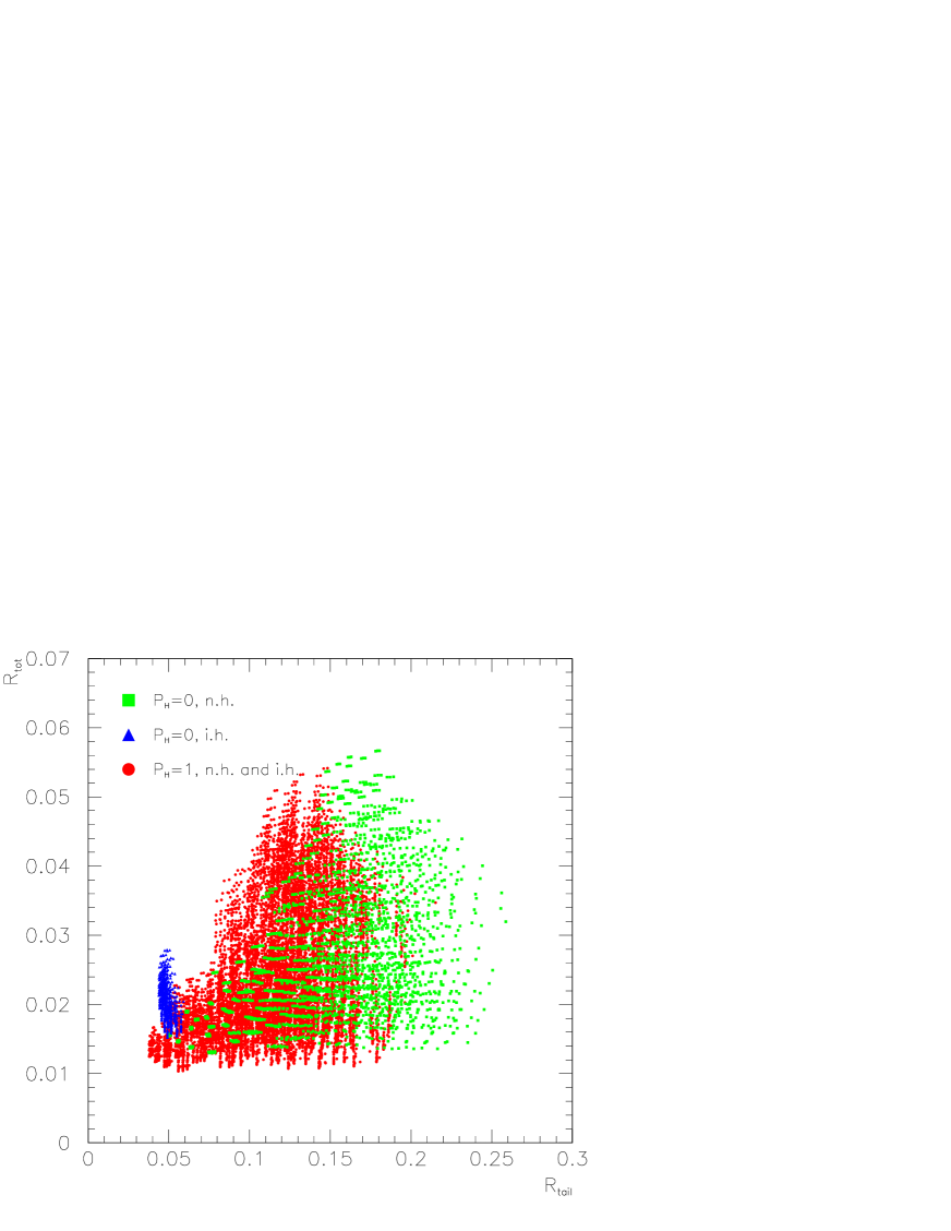
Figure 3: Scatter plot in the plane $R_{tail}-R_{tot}$ for the cases A, B and C discussed in sec. 5.1. The quantity $R_{tot}$ is the ratio of the total rates of $\mathrel{{\nu_{e}}}$ and $\mathrel{{\bar{\nu}}_{e}}$ events, eq. (58). The cuts $E_{L}=45$ MeV and $\bar{E}_{L}=55$ MeV were taken for $R_{tail}$.

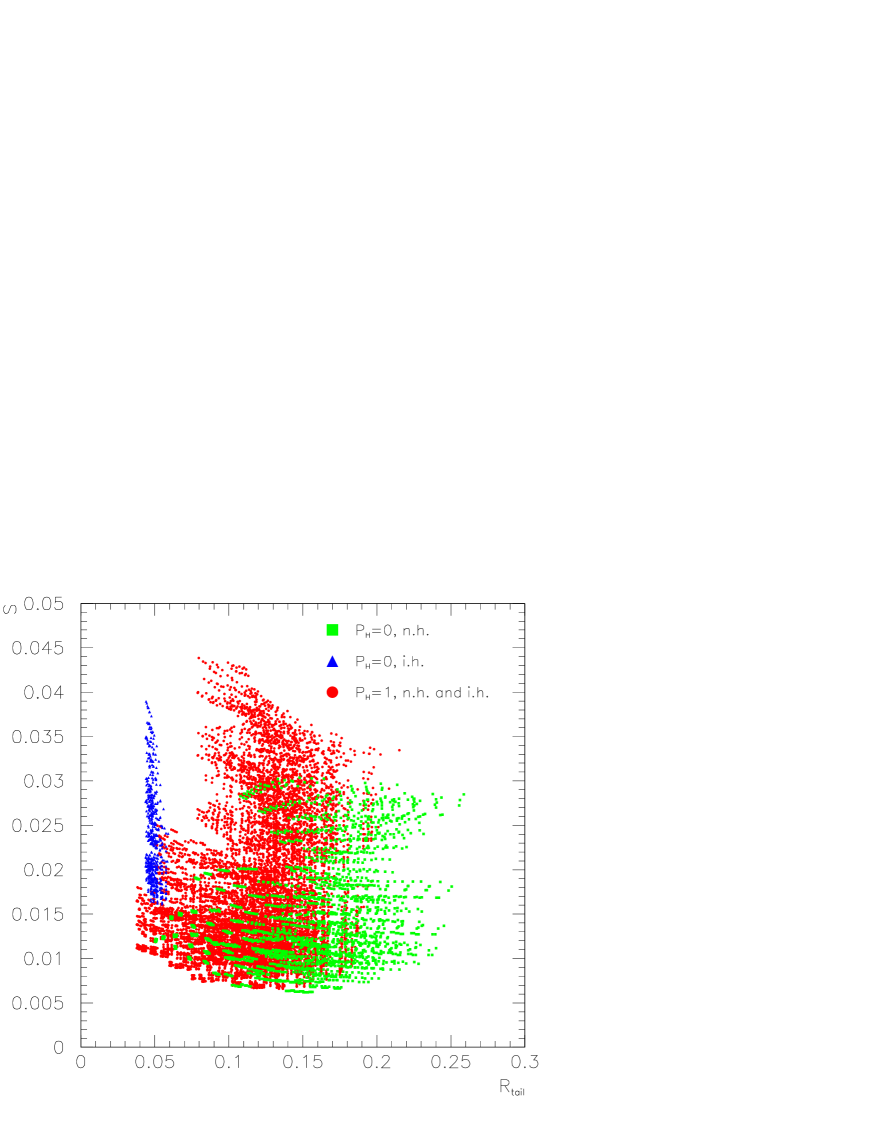
Figure 4: Same as fig. 3 in the $R_{tail}-S$ plane, where $S$ is defined according to eq. (53). We took the cuts $E^{\prime}_{L}=\bar{E}^{\prime}_{L}=25$ MeV for the calculation of $S$.

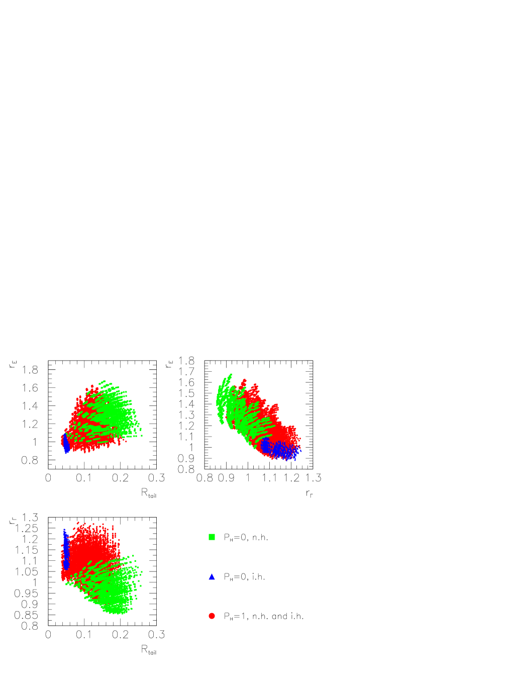
Figure 5: Scatter plots in the space of the variables: $R_{tail}$, $r_{E}$, $r_{\Gamma}$, eqs. (52), (41) and (42).

The results are shown in figs.  3 -5.

The fig. 3 shows the ($R_{tot}-R_{tail}$) scatter plot. The ratio of events in the tails, $R_{tail}$, is defined in (52) and $R_{tot}$ is the ratio of the total numbers of neutrino and antineutrino events:

$$R_{tot}\equiv\frac{N_{tot}}{\bar{N}_{tot}}~{},$$ (58)

where $N_{tot}$ for neutrinos is defined in (38). From the figure it follows that in the case B the ratio $R_{tot}$ can not exceed $\sim 0.032$, while for C $R_{tot}$ can be nearly twice as large. The difference is explained by the different degree of permutation in the various cases, according to what discussed in sec. 5.1. In case B the observed antineutrino spectrum is completely permuted and therefore maximally hard. This in turn implies the largest rate of $\mathrel{{\bar{\nu}}_{e}}$ events due to the larger detection cross section at high energies. In the case C the permutation of $\mathrel{{\bar{\nu}}_{e}}$ is partial, giving softer observed $\mathrel{{\bar{\nu}}_{e}}$ spectrum and therefore smaller event rate and larger value of $R_{tot}$. The $\mathrel{{\nu_{e}}}$ spectrum is partially permuted in B and C, while in case A it is totally permuted and therefore harder. This implies a larger $R_{tot}$ with respect to C. Numerically the difference between the two cases is small (see figure), because in C the amount of permutation for $\mathrel{{\nu_{e}}}$ is rather large: $1-p\simeq\cos^{2}\theta_{12}\simeq 0.75$, making this case close to complete permutation.

The parameter $R_{tail}$ has much higher discriminative power than $R_{tot}$. $R_{tail}<0.06$ for the case B and practically there is no overlap of the regions A and B. The region C overlaps with both A and B, although for $R_{tail}>0.22$ only A is allowed.

As follows from the figure, there are certain regions in the $R_{tail}-R_{tot}$ plane where only one possibility is realized. For the case of inverted mass hierarchy and large $\theta_{13}$ (B), the region is defined as $R_{tail}=(0.040-0.055)$, $R_{tot}=(0.02-0.03)$. For the case of very small 13-mixing (C) there is a band around $R_{tot}\simeq(0.3\cdot R_{tail})$ with $R_{tail}<(0.05-0.14)$. The normal mass hierarchy case A is the unique possibility for $R_{tail}>(0.14-0.22)$ where the border depends on value of $R_{tot}$.

Clearly it will be easy to identify or discriminate the case B. It might be more difficult to disentangle A and C since a significant overlap exists. The overlapping areas correspond to similar original fluxes in the different neutrino flavors: conversion effects are smaller for smaller difference of the original fluxes, making it difficult to disentangle different scenarios of mass hierarchy and 13-mixing.

The fig. 4 shows the $S-R_{tail}$ scatter plot, where the ratio of the numbers of low energy events, $S$, is defined in (53). This figure is rather similar to fig. 3, although the $S$ parameter is more complementary to $R_{tail}$ than $R_{tot}$, and experimentally $S$ and $R_{tail}$ are independent. The case B has higher $S$ and smaller $R_{tail}$, inversely, the scenario A predicts higher $R_{tail}$ and smaller $S$. The case C is intermediate between the two. As a consequence, the overlap of regions is smaller than in fig. 3.

We find the following regions where only one possibility is realized: The case A is unique for $R_{tail}>0.165$, the case B is unique for $S>0.017$ and $R_{tail}=(0.040-0.055)$, and C is unique in the band $S\approx(0.2-0.3)\cdot R_{tail}$.

These features are explained in terms of total or partial permutation, similarly to what we have dicussed for fig. 3.

The figure 5 shows scatter plots in the space of the variables $R_{tail}$, $r_{E}$ (41), and $r_{\Gamma}$ (42). The corresponding intervals of values of these observables for each of the scenarios A, B, C are summarized in the Table 1. For comparison, the Table displays also the expected intervals of the same variables for the neutrino spectra discussed in sec. 5.1. These parameters are not observable, however they allow to understand the features of the observable spectra.

parameter $\backslash$ scenario	A	B	C
$r_{E}$(events)	1.0 - 1.7	0.87 - 1.1	0.9 - 1.6
$r_{E}$(neutrinos)	$>$ 1	$<$ 1	$\mathrel{\vbox{\hbox{$>$}\nointerlineskip\hbox{$\sim$}}}$ 1
$r_{\Gamma}$(events)	0.85 - 1.1	1.06 - 1.25	0.9 - 1.25
$r_{\Gamma}$(neutrinos)	$\mathrel{\vbox{\hbox{$<$}\nointerlineskip\hbox{$\sim$}}}$ 1	$\mathrel{\vbox{\hbox{$>$}\nointerlineskip\hbox{$\sim$}}}$ 1	$\mathrel{\vbox{\hbox{$>$}\nointerlineskip\hbox{$\sim$}}}$ 1
$R_{tail}$	0.04 - 0.26	0.04 - 0.056	0.035 - 0.21

Table 1: The ranges of parameters of the spectra of observable events (“events”) for three possible cases of mass hierarchy and 1-3 mixing. For comparison we present also the corresponding characteristics of the neutrino spectra (“neutrinos”), which are not immediate observables.

From the figure and the Table it follows that for the case B the allowed region of parameters is relatively small, while for A and C the allowed regions are larger and expand over $r_{E}\simeq 1-1.5$. Furthermore, $r_{\Gamma}$ is mostly larger than 1 in C and mostly smaller than 1 in A. These results largely follow the expectations for the neutrino spectra, and can be interpreted in terms of the amount of permutation according to the discussion in sec. 5.1.

One can see two slight deviations with respect to the predictions for neutrino spectra: (1) a significant number of points with $r_{E}>1$ in the case B and (2) an appreciable amount of points with $r_{\Gamma}>1$ for the case A. The latter is in agreement with the possibility that the broadening of the spectrum due to compositeness is overcompensated by the effect of pinching, as commented in sec. 5.1. Moreover, the following reasons contribute to explain the deviations:

(i) the small contribution of the original $\mathrel{{\nu_{e}}}$ flux in the detected $\mathrel{{\nu_{e}}}$ signal. This contribution is – depending on the value of $\theta_{13}$ – not larger than $\sin^{2}\theta_{12}\simeq 0.25$, therefore the average energy of the observed $\mathrel{{\nu_{e}}}$ spectrum is dominated by the harder component due to the original $\mathrel{{\nu_{x}}}$ flux.

(ii) the different energy dependence of the cross sections of the $\mathrel{{\bar{\nu}}_{e}}+p$ and $\mathrel{{\nu_{e}}}+d$ detection reactions: the first grows like $E^{2}$ with suppressing corrections at high energies [61, 62], while the second has a stronger growth with energy, being proportional to $E^{2.25}$ [60]. It follows that in presence of equal $\mathrel{{\nu_{e}}}$ and $\mathrel{{\bar{\nu}}_{e}}$ energy spectra, this difference leads to higher average energy and larger width of the observed $\mathrel{{\nu_{e}}}$ spectrum.

Large regions of the parameter space exist where only one among the scenarios A, B or C is possible. Also regions appear when two of these scenarios are realized. If these regions are selected by the experiments, the third possibility will be excluded. From the figs. 3-5 we conclude that:

• The case A is excluded if observations give $R_{tail}\mathrel{\vbox{\hbox{$<$}\nointerlineskip\hbox{$\sim$}}}0.06$ and/or $r_{\Gamma}\mathrel{\vbox{\hbox{$>$}\nointerlineskip\hbox{$\sim$}}}1.1$. If, in contrast, the experiments give $R_{tail}>0.22$ the normal hierarchy would be identified. This result would be further supported if $r_{\Gamma}\mathrel{\vbox{\hbox{$<$}\nointerlineskip\hbox{$\sim$}}}0.95$ is also found.

  The possibility of getting information on $P_{H}$ and consequently on $\theta_{13}$ depends on the specific value of $R_{tail}$ (as illustrated in sec. 6).

• The case B is excluded by large values of $R_{tail}$ and large values of the ratio of average energies: $R_{tail}\mathrel{\vbox{\hbox{$>$}\nointerlineskip\hbox{$\sim$}}}0.06$ and $r_{E}\mathrel{\vbox{\hbox{$>$}\nointerlineskip\hbox{$\sim$}}}1.2$. The identification of this scenario (and therefore of the inverted mass hierarchy) appears difficult due to the almost complete overlap with the regions of the case C. Another indication of this scenario would be the result $r_{E}<0.95$. Again, conclusions on $\theta_{13}$ depend on the specific value of $R_{tail}$.

• The case C can not be easily identified. An indication of this possibility would be the result $r_{E}\mathrel{\vbox{\hbox{$>$}\nointerlineskip\hbox{$\sim$}}}1.2$ and $r_{\Gamma}\mathrel{\vbox{\hbox{$>$}\nointerlineskip\hbox{$\sim$}}}1.05$. This combination would exclude B and A, and therefore indicate $P_{H}>0$, corresponding to small values of $\theta_{13}$: $\mathrel{{\sin^{2}\theta_{13}}}\mathrel{\vbox{\hbox{$<$}\nointerlineskip\hbox{$\sim$}}}few\cdot 10^{-4}$ (see fig. 1).
  

The scenarios in which $0<P_{H}<1$ are not shown in the figures. For n.h. and $0<P_{H}<1$ we expect the allowed region to be intermediate between the regions found for A and C. Similarly, for i.h. and $0<P_{H}<1$ the region of possible values of parameters is intermediate between the regions of cases B and C. For this reason, the conclusions we derived from the figures 3-5 have essentially an exclusion character and not the character of establishing one of the scenarios A, B, C.

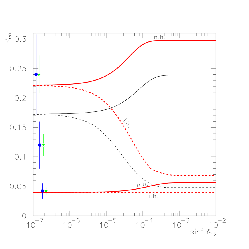
Figure 10: The ratio $R_{tail}$ as a function of $\mathrel{{\sin^{2}\theta_{13}}}$ for normal mass hierarchy (solid lines) and inverted hierarchy (dashed lines), in absence of Earth crossing. The bands within the thick lines represent the values that $R_{tail}$ can take once all the possible theoretical uncertainties are considered (see text). The thin lines refer to the “ideal” case $\alpha=\bar{\alpha}=0$. We have taken $\mathrel{{\tan^{2}\theta_{12}}}=0.38$, $E_{L}=45$ MeV and ${\bar{E}}_{L}=55$ MeV. Three examples of experimental results for $R_{tail}$ are shown with two different (98% C.L.) error bars (marked by bullets and stars) corresponding to $T_{x}=7$ MeV, $L_{e}=L_{\bar{e}}=L_{x}=L_{\bar{x}}=5\cdot 10^{52}$ ergs, and $D=8.5$ kpc and $D=4$ kpc respectively.

It is clear that the potential of the method we have discussed depends on the statistics and therefore on the distance from the supernova. Some estimations are presented in sec. 6.6 and fig. 10. For a relatively close star ($D\mathrel{\vbox{\hbox{$<$}\nointerlineskip\hbox{$\sim$}}}4$ kpc) the error bars are substantially smaller than the field of points so that the discrimination of different possibilities becomes possible.

It is easy to understand the effect on the scatter plots of choosing more conservative intervals of the parameters of the original neutrino fluxes. In particular, for smaller differences of the average energies in the different flavors the spectral distortions due to conversion become smaller (see e.g. [5]). The results approach those expected in absence of conversion and therefore are the same in the three secenarios, A, B, C. The corresponding points in the scatter plots would be located where the regions for the three cases are closer or overlap. Clearly, any sensitivity to the neutrino mixings and mass hierarchy is lost in this situation.

6 The method of the high energy tails

6.1 $R_{tail}$ and $r$.

The uncertainties related to the original neutrino fluxes can be substantially reduced if

• ratios of the electron neutrino and antineutrino signals are considered;

• the high energy tails of spectra are used.

The key point is that in the high energy tails the fluxes of non-electron neutrinos dominate, and moreover, these fluxes are nearly equal.

In what follows we study the possibility to use the ratio $R_{tail}(E_{L},\bar{E}_{L})$ introduced in (52) to establish the mass hierarchy and to probe $\theta_{13}$. As we have seen in the previous sections the dependences of the neutrino and antineutrino signals on $\theta_{13}$ and on the sign of $\Delta m^{2}_{13}$ are different.

Let us consider the predictions for $R_{tail}$ in details. This ratio can be written in terms of the original neutrino fluxes and the survival probabilities $p$ and $\bar{p}$ as:

$$R_{tail}(E_{L},\bar{E}_{L})\simeq{1-\langle p\rangle+\alpha(E_{L})\langle p\rangle\over 1-\langle{\bar{p}}\rangle+\bar{\alpha}(\bar{E}_{L})\langle\bar{p}\rangle}~{}Q(E_{L},\bar{E}_{L})~{}.$$ (59)

Here the brackets $\langle\rangle$ denote the averaging over the corresponding energy intervals (we have taken into account the weak energy dependence of $p$ and $\bar{p}$).

The quantity $Q$ is defined as:

$$Q(E_{L},\bar{E}_{L})\equiv\frac{N_{x}^{0}(E>E_{L})}{N_{\bar{x}}^{0}(E>\bar{E}_{L})}~{},$$ (60)

where $N_{x}^{0}$, $N_{\bar{x}}^{0}$ are the numbers of events calculated according to eqs. (47) and (31) with the fluxes $F_{x}^{0}$ and $F_{\bar{x}}^{0}$ respectively. Due to the near equality of the fluxes $F^{0}_{x}$ and $F^{0}_{\bar{x}}$, the astrophysical uncertainties in $Q$ are almost cancelled for an optimized choice of the cuts $E_{L}$ and $\bar{E}_{L}$ (see sect. 6.2).

In (59) $\alpha$ and $\bar{\alpha}$ are the parameters which describe the relative contributions of the original $\nu_{e}$ and $\bar{\nu}_{e}$ fluxes to the numbers of events above the energy cuts:

$$\alpha(E_{L})\equiv\frac{N^{0}_{e}(E_{L})}{N^{0}_{x}(E_{L})}~{},\hskip 28.45274pt\bar{\alpha}(\bar{E}_{L})\equiv\frac{N^{0}_{\bar{e}}(\bar{E}_{L})}{N^{0}_{\bar{x}}(\bar{E}_{L})}~{}.$$ (61)

Let us introduce the ratio:

$$r(E_{L},\bar{E}_{L})\equiv\frac{R_{tail}(E_{L},\bar{E}_{L})}{Q(E_{L},\bar{E}_{L})}~{},$$ (62)

which should not depend substantially on the features of the detectors, and is known once $R_{tail}$ is measured. According to (59) we have:

$$r(E_{L},\bar{E}_{L})\simeq{1-\langle p\rangle(1-\alpha(E_{L}))\over 1-\langle{\bar{p}}\rangle(1-\bar{\alpha}(\bar{E}_{L}))}~{}.$$ (63)

The ratio $R_{tail}$ is a measurable quantity, and, as we will argue in the next section, $Q(E_{L},\bar{E}_{L})$ can be reliably predicted. Therefore, the study of $R_{tail}$ can be reduced to that of the quantity $r(E_{L},\bar{E}_{L})$.

6.2 The factor $Q$

The factor $Q(E_{L},\bar{E}_{L})$ depends on (i) the energy cuts $E_{L}$ and ${\bar{E}_{L}}$, (ii) the fluxes $F^{0}_{x}$ and $F^{0}_{\bar{x}}$ and (iii) on the features of the detection method: cross sections, efficiencies, energy resolutions, etc. (for the latter quantities we follow ref. [65]). Since $F^{0}_{x}$ and $F^{0}_{\bar{x}}$ have almost equal luminosities, temperatures and pinching parameters, the astrophysical uncertainties affect $Q$ only weakly. Moreover, the effect of uncertainties can be further suppressed by choosing different thresholds for neutrino and antineutrino events, such to “compensate” the difference in the temperatures.

This can be seen from the approximate form of the ratio $Q$ (eq. (60)):

$$Q \simeq const~{}\frac{T_{x}}{T_{\bar{x}}}\frac{P(E_{L}/T_{x})}{P(\bar{E}_{L}/T_{\bar{x}})}e^{(-E_{L}/T_{x}+\bar{E}_{L}/T_{\bar{x}})}~{},$$ (64)

$$\sim const~{}\left(\frac{T_{\bar{x}}}{T_{x}}\right)^{3}\left(\frac{E_{L}}{\bar{E}_{L}}\right)^{4}e^{(-E_{L}/T_{x}+\bar{E}_{L}/T_{\bar{x}})}~{},$$ (65)

which can be derived from the analytical formulas (49, 51). In eq. (65) we took $L_{\bar{x}}=L_{x}$ and $\eta_{x}=\eta_{\bar{x}}$. For simplicity we considered the same energy dependence of the $\mathrel{{\nu_{e}}}$ and $\mathrel{{\bar{\nu}}_{e}}$ cross-sections, $\sigma(\nu)\propto\sigma(\bar{\nu})\propto E^{2}$, and neglected detector parameters like energy resolution, efficiency, etc.. From eq. (65) we see that if $T_{x}=T_{\bar{x}}$ the ratio $Q$ reduces to a constant provided that $E_{L}=\bar{E}_{L}$ is taken. In the presence of a difference $\delta_{x}$ between the $\mathrel{{\nu_{x}}}$ and $\mathrel{{\bar{\nu}}_{x}}$ temperatures, eq. (3), the dependence of $Q$ on $T_{x}$ does not cancel exactly. However, one can find values of the energy cuts, $E_{L}\neq\bar{E}_{L}$, for which this dependence becomes very weak in the relevant range of $T_{x}$:

$$\frac{\partial Q}{\partial T_{x}}\approx 0\hskip 56.9055pt{\rm for}~{}~{}~{}T_{x}=(5\div 8)~{}{\rm MeV}~{}.$$ (66)

In the approximation $\delta_{x}/T_{x}\ll 1$ and $\bar{E}_{L}/E_{L}-1\ll 1$, Eqs. (65) and (66) lead to

$$\frac{\bar{E}_{L}}{E_{L}}\simeq 1+\frac{\delta_{x}}{T_{x}}\left(2-3\frac{T_{x}}{E_{L}}\right)~{}.$$ (67)

Taking $E_{L}=45$ MeV, $T_{x}=7$ MeV and $\delta_{x}=0.5$ MeV, from (67) we get $\bar{E}_{L}\simeq 50$ MeV. A more detailed numerical study, which takes into account also the different energy dependences of the cross-sections, give $\bar{E}_{L}\simeq 55$ MeV.

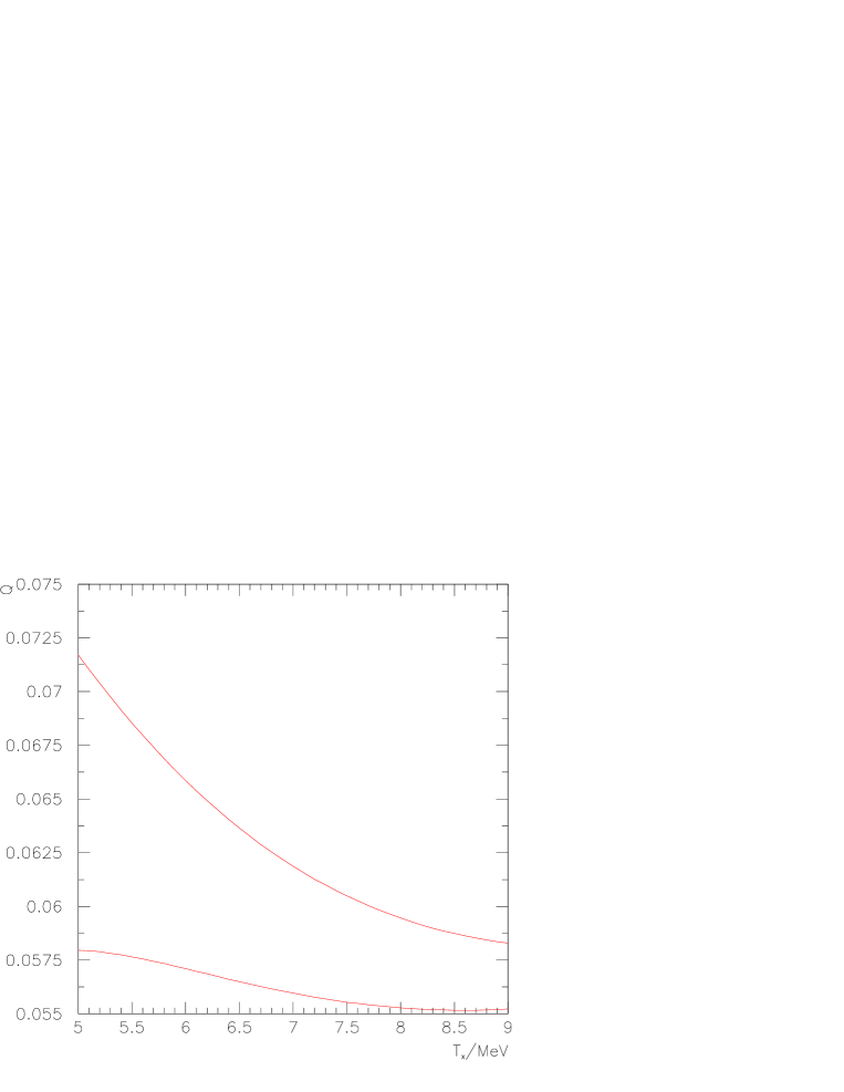
Figure 6: The factor $Q$ (region between the lines), eq. (60), as a function of the temperature $T_{x}$. The width of the region corresponds to the interval $T_{\bar{x}}-T_{x}=0.35\div 0.5$ MeV. The cuts $E_{L}=45$ MeV and $\bar{E}_{L}=55$ MeV have been taken.

The dependence of the factor $Q$ on the temperature $T_{x}$ is shown in fig. 6 (region between the lines), for $E_{L}=45$ MeV, $\bar{E}_{L}=55$ MeV and $\delta_{x}=0.35\div 0.5$ MeV. As it appears from the figure, over the interval $T_{x}=5\div 9$ MeV, $Q$ varies by about $\sim 10\%$ of its value, therefore it can be taken as a constant with $\sim 10\%$ associated error:

$$Q=0.0635(1\pm 0.13)~{}.$$ (68)

As it can be understood from eqs. (65) and (67), the error on $Q$ is dominated by the uncertainty in the value of $\delta_{x}$: fixing $\delta_{x}=0.5$ MeV we get $Q=0.0566(1\pm 0.05)$ in the relevant interval of values of $T_{x}$.

6.3 $\alpha$ and $\bar{\alpha}$. Threshold Energies

The ratios $\alpha$ and $\bar{\alpha}$, eq. (61), depend (i) on the features of the original electron and non electron neutrino fluxes, (ii) on the energy cuts $E_{L}$, $\bar{E}_{L}$ and (iii) on the characteristics of the detectors consider. Using the Maxwell-Boltzmann approximation, eq. (48), and the results (49,50), one gets the following approximate expression for $\alpha$:

$$\alpha\simeq\frac{L_{e}T_{e}}{L_{x}T_{x}}\frac{P(E_{L}/T_{e})}{P(E_{L}/T_{x})}e^{-E_{L}(1/T_{e}-1/T_{x})}~{},$$ (69)

where the dependence $\sigma(\nu)\propto E^{2}$ has been considered and other detection parameters (efficiency, energy resolution, etc.) neglected. The polynome $P(x)$ is given in eq. (50). The dependence of ratio $P(E_{L}/T_{e})/P(E_{L}/T_{x})$ on $E_{L}$ is weak and cancels in the asymptotics $E_{L}\gg T_{e},T_{x}$. In this limit we have:

$$\alpha\approx\frac{L_{e}}{L_{x}}\left(\frac{T_{x}}{T_{e}}\right)^{3}e^{-E_{L}(1/T_{e}-1/T_{x})}~{}.$$ (70)

From eqs. (69, 70) it follows that, for a given $T_{x}$, the ratio $\alpha$ decreases with the decrease of $T_{e}$ and with the increase of the cut $E_{L}$. We have $\alpha\rightarrow 0$ in the limit $E_{L}/T_{e}\rightarrow\infty$. In particular, this implies that the contribution of $\alpha$ to the ratio $r$ (eq. (63)) can be reduced to a small correction provided that a high enough cut is chosen.

Results analogous to eqs. (69, 70) and similar considerations hold for $\bar{\alpha}$. As a consequence of inequalities of the average energies, eq. (2), and of the nearly equality of luminosities we have

$$\bar{\alpha}(\bar{E}_{L})>\alpha(E_{L})~{},$$ (71)

provided that $\bar{E}_{L}$ and $E_{L}$ do not differ strongly.

Though approximate, the expression (69) is in acceptable agreement with more accurate numerical calculations. Scanning the intervals of parameters of the original neutrino spectra (2 - 4) we find the following ranges of $\alpha$ and $\bar{\alpha}$:

$$\alpha(45{\rm MeV})\simeq 0-0.42~{},~{}~{}~{}~{}~{}\bar{\alpha}(55{\rm MeV})\simeq 0-0.95~{}.$$ (72)

As an example, taking the “traditional” scenario with equal luminosities in the different flavors and hierarchical (unpinched) spectra – with $T_{x}=7$ MeV, $T_{\bar{e}}=5$ MeV and $T_{e}=3.5$ MeV – we get

$$\alpha(45{\rm MeV})\simeq 0.05,~{}~{}~{}~{}~{}\bar{\alpha}(55{\rm MeV})\simeq 0.16.$$ (73)

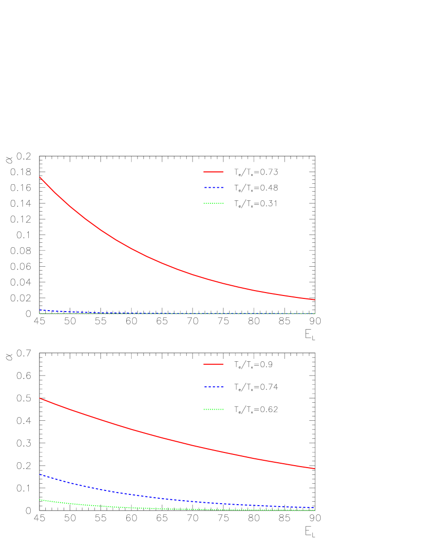
Figure 7: The dependence of the ratios $\alpha$ (upper panel) and $\bar{\alpha}$ (lower panel), eq. (61), on the energy cuts $E_{L}$ and $\bar{E}_{L}$ respectively, for $T_{x}=7$ MeV, $L_{e}=L_{\bar{e}}=L_{x}$, $\eta_{e}=\eta_{\bar{e}}=\eta_{x}=0$ and different values of the $\mathrel{{\nu_{e}}}$ and $\mathrel{{\bar{\nu}}_{e}}$ temperature (expressed in term of ratios in the legend).

In fig. 7 we show the dependence of $\alpha$ and $\bar{\alpha}$ on the cut energies, $E_{L}$ and $\bar{E}_{L}$, for $T_{x}=7$ MeV, $L_{e}=L_{\bar{e}}=L_{x}$, $\eta_{e}=\eta_{\bar{e}}=\eta_{x}=0$ and different values of the $\mathrel{{\nu_{e}}}$ and $\mathrel{{\bar{\nu}}_{e}}$ temperature. It can be seen that the decrease of $\alpha$ and $\bar{\alpha}$ with the cuts is indeed exponential, in agreement with eq. (69). However, if the hierarchy of the spectra is not strong (solid lines in the figure), for our choice of the cuts $\alpha$, and especially $\bar{\alpha}$, are not negligible with respect to the survival probabilities: $\alpha\mathrel{\vbox{\hbox{$<$}\nointerlineskip\hbox{$\sim$}}}\bar{\alpha}\sim p,\bar{p}\mathrel{\vbox{\hbox{$<$}\nointerlineskip\hbox{$\sim$}}}1$. In this case, the effects of the $\alpha$ and $\bar{\alpha}$ terms in $r$ (and therefore in $R_{tail}$) can be reduced by adopting higher energy cuts. According to fig. 7, requiring $\alpha\mathrel{\vbox{\hbox{$<$}\nointerlineskip\hbox{$\sim$}}}\bar{\alpha}\mathrel{\vbox{\hbox{$<$}\nointerlineskip\hbox{$\sim$}}}0.1$ implies $E_{L}\mathrel{\vbox{\hbox{$<$}\nointerlineskip\hbox{$\sim$}}}70$ MeV and $\bar{E}_{L}\mathrel{\vbox{\hbox{$<$}\nointerlineskip\hbox{$\sim$}}}100-120$ MeV (we have considered the possibility, not shown in the figure, to have $L_{e}/L_{x}\simeq 2$ and/or $L_{\bar{e}}/L_{x}\simeq 2$, corresponding to twice as large values of $\alpha$ and $\bar{\alpha}$ with respect to what shown in the figure). It is clear, however, that the numbers of events in the tails above these energies is strongly suppressed, so that no precise measurements of $r$ are possible.

6.4 Large threshold energy limit

For $E_{L}\gg\langle E_{e}\rangle,\langle E_{\bar{e}}\rangle$ parameters $\alpha,~{}\bar{\alpha}$ are negligible and expression (63) becomes

$$r\approx{1-\langle p\rangle\over 1-\langle{\bar{p}}\rangle}~{},$$ (74)

i.e. the astrophysical and oscillation parts of $R_{tail}$ are factorized.

Inserting the explicit expressions for the permutation factors, eqs. (20 - 23), and neglecting $\sim\mathrel{{\sin^{2}\theta_{13}}}$ terms, we find

$$r=\frac{1}{\sin^{2}\theta_{12}}-\langle P_{H}~{}\rangle~{}~{}~{}~{}{\rm(n.h.)},$$ (75)

$$r=\frac{1}{\cos^{-2}\theta_{12}-\langle P_{H}~{}\rangle}~{}~{}~{}~{}~{}{\rm(i.h.)},$$ (76)

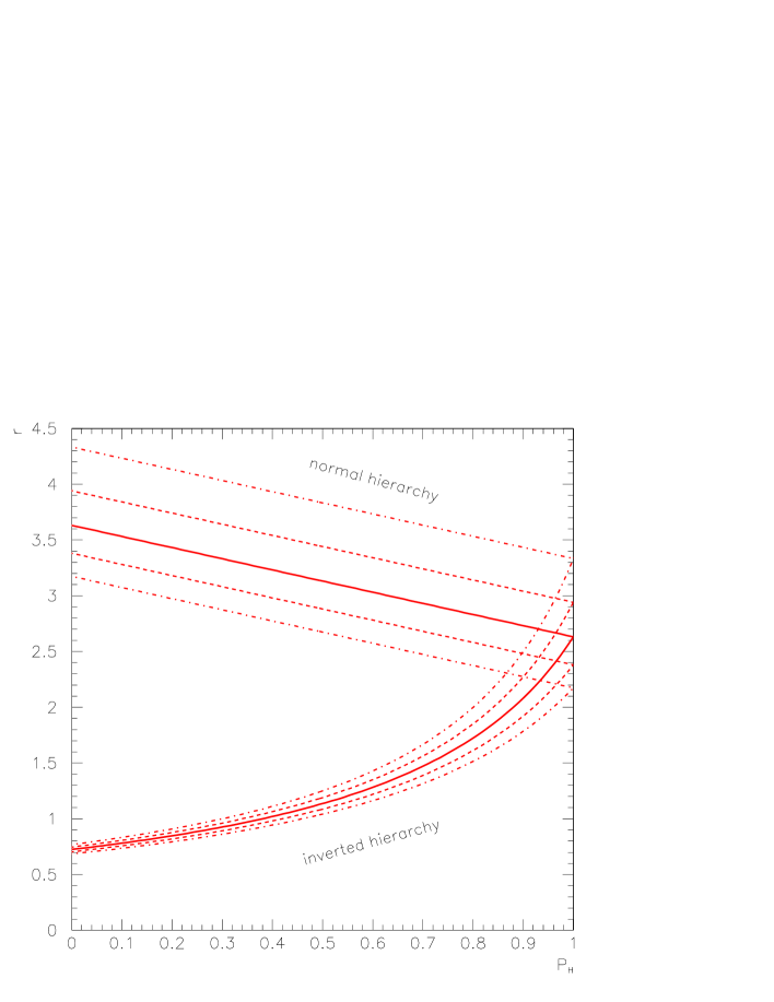
Figure 8: The factor $r$, eq. (74), as a function of $P_{H}$ for $\mathrel{{\tan^{2}\theta_{12}}}=0.38$ and both normal and inverted hierarchy (solid line). The bands within the dashed and dashed-dotted lines correspond to $10\%$ and $20\%$ uncertainty on $\mathrel{{\tan^{2}\theta_{12}}}$ respectively.

where $\langle P_{H}~{}\rangle$ is the value of the jumping probability averaged over the energy interval under consideration. The ratio $r$ is shown in fig. 8 as a function of $\langle P_{H}~{}\rangle$ for different values of $\mathrel{{\tan^{2}\theta_{12}}}$. In the limit of $\langle P_{H}\rangle\rightarrow 1$, i.e. very small $\theta_{13}$, we get

$$r_{1}=\frac{1}{\tan^{2}\theta_{12}}~{}$$ (77)

for both hierarchies. In general one finds

$$r~{}\begin{cases}\geq 1/\mathrel{{\tan^{2}\theta_{12}}}&~{}~{}~{}\text{(n.h.)}\\ \leq 1/\mathrel{{\tan^{2}\theta_{12}}}&~{}~{}~{}\text{(i.h.)}\end{cases}~{},$$ (78)

and in the limit $\langle P_{H}\rangle\rightarrow 0$ (large $\theta_{13}$)

$$r\rightarrow r_{0}=\begin{cases}1/\sin^{2}\theta_{12}&~{}~{}\text{(n.h.)}\\ \cos^{2}\theta_{12}&~{}~{}\text{(i.h.)}\end{cases}~{}.$$ (79)

For both the hierarchies $r$ decreases with the increase of the mixing $\theta_{12}$.

Once (i) $R_{tail}$ is measured in experiments, (ii) $Q$ is calculated and (iii) $\mathrel{{\tan^{2}\theta_{12}}}$ is known from the solar neutrino and the KamLAND experiments, the inequalities (78) can be used to establish the mass hierarchy. Assuming that $\mathrel{{\tan^{2}\theta_{12}}}$ will be measured with $20\%$ accuracy, from the figure 8 (see dash-dotted lines; the central value $\mathrel{{\tan^{2}\theta_{12}}}=0.38$ has been taken as an example) we find that:

1). If $r<2$ the inverted hierarchy will be selected. In particular, if $r\sim 0.7$ even a poor accuracy in measurements of $r$, say $30-50\%$, will be enough. Moreover, the (energy-averaged) jump probability will be restricted: $\langle P_{H}\rangle<0.3$, leading to a lower bound on $\mathrel{{\sin^{2}\theta_{13}}}$.

2). If $r=(2.0-3.5)$ both types of hierarchy are possible. For inverted hierarchy one can put a rather strong bound on the jumping probability: $\langle P_{H}\rangle>0.8$, which would imply an upper bound on $\tan^{2}\theta_{13}$. In the case of normal hierarchy no bound on $P_{H}$ appears.

3). For $r>3.5$ the normal hierarchy with $\langle P_{H}\rangle<1$ is selected.

According to eqs. (75)-(76) we have:

$$\langle P_{H}\rangle=\frac{1}{\sin^{2}\theta_{12}}-r~{}~{}~{}~{}~{}{\rm(n.h.)},$$ (80)

$$\langle P_{H}\rangle=\frac{1}{\cos^{2}\theta_{12}}-\frac{1}{r}~{}~{}~{}~{}~{}{\rm(i.h.)}.$$ (81)

The result for $\langle P_{H}\rangle$ can be then transferred into a result for $\tan^{2}\theta_{13}$ using fig. 1 and the expressions (13, 14). As follows from the fig. 1, even for very precise measurements of $\langle P_{H}\rangle$ the uncertainty on the density profile will lead to a factor of 3 uncertainty on $\mathrel{{\sin^{2}\theta_{13}}}$. To have a sensitivity to $\sin^{2}\theta_{13}$ in the adiabatic region one needs to measure the permutation effects at the level 2% or smaller. This looks practically impossible already in view of uncertainties on the determination of $\tan^{2}\theta_{12}$.

6.5 The general case

To have significant statistics in the tails the energy cuts should not be too large. In this case $\alpha$, $\bar{\alpha}$ can not be neglected and for the ratio $r$ we should use the complete expression (63). It can be rewritten in terms of the average jumping probability $\langle P_{H}\rangle$ and $\theta_{12}$ as

$$r=\frac{1+\tan^{2}\theta_{12}-\langle P_{H}\rangle\tan^{2}\theta_{12}(1-\alpha)}{\tan^{2}\theta_{12}+\bar{\alpha}}~{}~{}~{}~{}~{}~{}{\rm(n.h.)},$$ (82)

$$r=\frac{1+\alpha\tan^{2}\theta_{12}}{1+\tan^{2}\theta_{12}-\langle P_{H}\rangle(1-\bar{\alpha})}~{}~{}~{}~{}~{}~{}{\rm(i.h.)}.$$ (83)

For very small $\theta_{13}$ ($P_{H}=1$) both hierarchies give the same result:

$$r_{1}=\frac{1+\tan^{2}\theta_{12}\alpha}{\tan^{2}\theta_{12}+\bar{\alpha}}~{}.$$ (84)

Comparing $r_{1}$ with the general expressions (82, 83) we get the inequalities

$$r>r_{1}~{}~{}{\rm(n.h.)},~{}~{}~{}~{}~{}~{}~{}r<r_{1}~{}~{}{\rm(i.h.)}~{},$$ (85)

which provide a test of the type of mass hierarchy.

In the adiabatic case ($P_{H}\approx 0$):

$$r_{0}^{(n)}=\frac{1+\tan^{2}\theta_{12}}{\tan^{2}\theta_{12}+\bar{\alpha}}~{}~{}~{}~{}~{}~{}{\rm(n.h.)},$$ (86)

$$r_{0}^{(i)}=\frac{1+\alpha\tan^{2}\theta_{12}}{1+\tan^{2}\theta_{12}}~{}~{}~{}~{}~{}~{}{\rm(i.h.)}.$$ (87)

These quantities turn out to be the upper (for n.h.) and the lower (for i.h.) bounds on $r$:

$$r_{1}\leq r\leq r_{0}^{(n)}~{}~{}~{}~{}~{}{\rm(n.h.)},$$ (88)

$$r_{0}^{(i)}\leq r\leq r_{1}~{}~{}~{}~{}~{}{\rm(i.h.)}.$$ (89)

The averaged probability, $\langle P_{H}\rangle$, can be expressed in terms of measurable quantities as:

$$\langle P_{H}\rangle=\frac{1}{(1-\alpha)}[1+\cot^{2}\theta_{12}-r(1+\bar{\alpha}\cot^{2}\theta_{12})]~{}~{}~{}~{}~{}{\rm(n.h.)}$$ (90)

$$\langle P_{H}\rangle=\frac{1}{(1-\bar{\alpha})}[1+\tan^{2}\theta_{12}-\frac{1}{r}(1+\alpha\tan^{2}\theta_{12})]~{}~{}~{}~{}~{}{\rm(i.h.)}.$$ (91)

We can define the energy $E_{av}$ in such a way that

$$\langle P_{H}\rangle\equiv P_{H}(E_{av}).$$ (92)

Using the Landau-Zener formula for $P_{H}$ we find expression for $\sin^{2}\theta_{13}$ in terms of observables:

$$\mathrel{{\sin^{2}\theta_{13}}}\simeq-2.05\cdot 10^{-5}\left({E_{av}\over{\rm MeV}}\right)^{2/3}\left({10^{-3}~{}{\rm eV}^{2}\over|\Delta m^{2}_{32}|}\right)^{2/3}C^{-1/3}\ln(\langle P_{H}\rangle)~{}~{}~{}~{}(a=n,i),$$ (93)

where $\langle P_{H}\rangle$ are given in Eqs. (90, 91).

6.6 Results

Let us first estimate the influence of $\alpha$ and $\bar{\alpha}$ on the ratio $r=r(\alpha,\bar{\alpha})$. We denote here and later by $x^{+}$ and $x^{-}$ the upper and lower edges of the uncertainty interval of the variable $x$ ($x=\alpha,~{}\bar{\alpha},...$). Using the general expressions for $r$, eq. (82), and taking into account the restriction (71) we find the upper ($r_{max}$) and the lower ($r_{min}$) bounds on $r$ for given values of $\theta_{12}$ and $P_{H}$. In the case of the n.h. we get

$$r_{min}(P_{H})\approx r(0,\bar{\alpha}^{+})=\frac{1+\tan^{2}\theta_{12}-\langle P_{H}\rangle\tan^{2}\theta_{12}}{\tan^{2}\theta_{12}+\bar{\alpha}^{+}},$$ (94)

$$r_{max}(P_{H})\approx r(0,0)=\frac{1}{\sin^{2}\theta_{12}}-\langle P_{H}\rangle$$ (95)

which coincides with expression in the high energy limit. Here the minimum values $\alpha^{-}$ and $\bar{\alpha}^{-}$ have been set to zero for simplicity.

For inverted hierarchy we find the lower limit:

$$r_{min}(P_{H})=r(0,\bar{\alpha}^{+})=\frac{1}{1+\tan^{2}\theta_{12}-\langle P_{H}\rangle(1-\bar{\alpha}^{+})}~{},$$ (96)

while, due to the restriction (71), the upper limit has a more complicated dependence

$$r_{max}(P_{H})\approx\begin{cases}r(\alpha^{+},\alpha^{+})=\left[1+\alpha^{+}\tan^{2}\theta_{12}\right]\left[1+\tan^{2}\theta_{12}-\langle P_{H}\rangle(1-\alpha^{+})\right]^{-1}&\text{ $P_{H}\leq\mathrel{{\tan^{2}\theta_{12}}}$}\\ r(0,0)=\left[1+\tan^{2}\theta_{12}-\langle P_{H}\rangle\right]^{-1}&\text{ $P_{H}>\mathrel{{\tan^{2}\theta_{12}}}$}\end{cases}~{}.$$ (97)

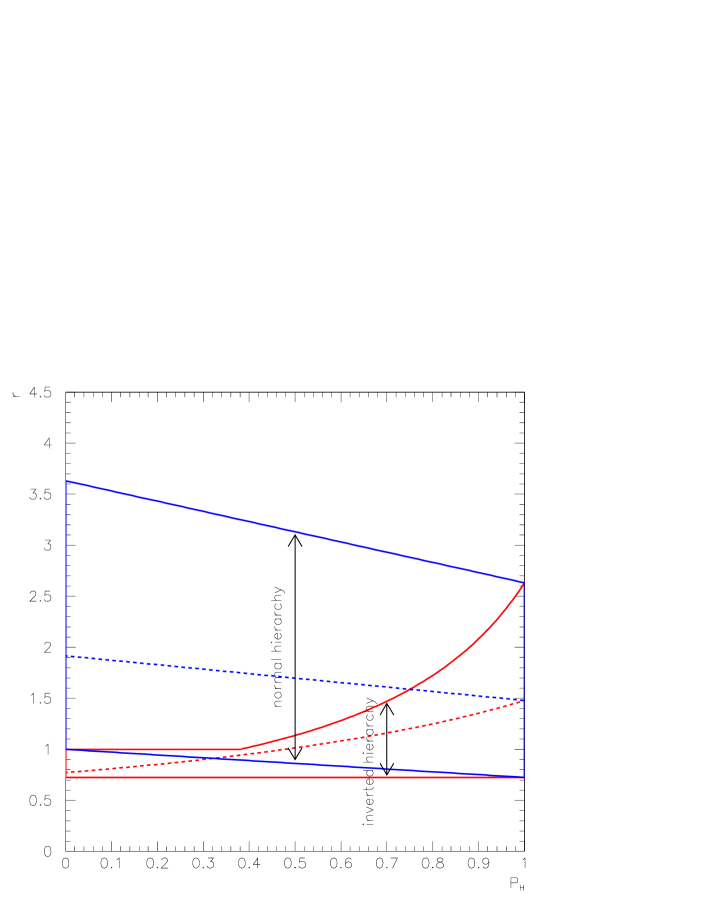
Figure 9: The same as fig. 8 where the assumption of hierarchy of the energy spectra has been relaxed to $\alpha\equiv N^{0}_{e}/N^{0}_{x}\leq 1$ and $\bar{\alpha}\equiv N^{0}_{\bar{e}}/N^{0}_{\bar{x}}\leq 1$ (eqs. (82)-(83)). The possible values of $r$ are those within the solid contours; the dashed lines correspond to $\alpha=0.17$ and $\bar{\alpha}=0.34$. We took $\mathrel{{\tan^{2}\theta_{12}}}=0.38$; for simplicity the effects of uncertainties on this parameter are not shown.

These limits are shown in fig. 9 for $\tan^{2}\theta_{12}=0.38$ and $\alpha^{+}=\bar{\alpha}^{+}=1$, together with predictions for $\alpha=0.17$ and $\bar{\alpha}=0.34$ as an example. As follows from the figure, with the present knowledge of the original spectra the mass hierarchy can be identified from the tail method only if

$$r>2.6$$ (98)

will be found. In this case also the upper bound on $\langle P_{H}\rangle$, and consequently a lower bound on $\sin^{2}\theta_{13}$ can be obtained:

$$\langle P_{H}\rangle\leq\frac{1}{\sin^{2}\theta_{12}}-r.$$ (99)

For $r<2.6$ neither the hierarchy nor $\sin^{2}\theta_{13}$ can be found. For the most plausible scenario (normal mass hierarchy, large $\sin^{2}\theta_{13}$ ($P_{H}=0$) we get $r\sim 2$, that is, below the identification interval.

More can be said if the hierarchy is identified by some other method (e.g., from the Earth matter effect or the shock wave effects, see secs. 6.7 and 7). Thus in the case of normal hierarchy, in addition to the upper bound (99), one can put a lower bound on $\langle P_{H}\rangle$ if $r=0.7-1$:

$$\langle P_{H}\rangle\geq\frac{1}{\sin^{2}\theta_{12}}-r\left(1+\frac{\bar{\alpha}^{+}}{\tan^{2}\theta_{12}}\right),$$ (100)

and, correspondingly, one gets an upper bound on $\sin^{2}\theta_{13}$.

If the inverted hierarchy is identified and $r=1-2.6$ is found, one can put a lower bound on $P_{H}$ (upper bound on $\sin^{2}\theta_{13}$):

$$\langle P_{H}\rangle\geq 1+\tan^{2}\theta_{12}-1/r.$$ (101)

The discrimination power increases with the increase of the low energy cut (i.e., decreases with $\alpha^{+}$ and $\bar{\alpha}^{+}$), however the statistics decreases fast correspondingly, so that such a possibility can be realized only in the case of supernova at small distances.

The features of $r$ are reproduced also in the observable $R_{tail}$, eq. (52). We find the minimal and maximal values of $R_{tail}=R_{tail}(E_{av},(|\Delta m^{2}_{32}|),C,\alpha,\bar{\alpha},\theta_{12},\theta_{13},Q)$ for a given $\theta_{13}$ taking into account also uncertainties on $\Delta m_{23}$, $\theta_{12}$, $C$, $E_{av}$. For the normal mass hierarchy, eqs. (94,95) and (13,14) give:

$$R_{max}(\theta_{13})=R(E^{-}_{av},(|\Delta m^{2}_{32}|)^{+},C^{+},0,0,\theta^{-}_{12},\theta_{13},Q^{+})$$

$$R_{min}(\theta_{13})=R(E^{+}_{av},(|\Delta m^{2}_{32}|)^{-},C^{-},0,\bar{\alpha}^{+},\theta^{+}_{12},\theta_{13},Q^{-})~{}.$$ (102)

Similarly, from eqs. (96,97) we get for inverted mass hierarchy:

$$R_{max}(\theta_{13})=\begin{cases}R(E^{+}_{av},(|\Delta m^{2}_{32}|)^{-},C^{-},\alpha^{+},\alpha^{+},\theta^{-}_{12},\theta_{13},Q^{+})&\text{ $P_{H}\leq\mathrel{{\tan^{2}\theta_{12}}}$}\\ R(E^{+}_{av},(|\Delta m^{2}_{32}|)^{-},C^{-},0~{}~{},0~{}~{},\theta^{-}_{12},\theta_{13},Q^{+})&\text{ $P_{H}>\mathrel{{\tan^{2}\theta_{12}}}$}\end{cases}$$

$$R_{min}(\theta_{13})=R(E^{-}_{av},(|\Delta m^{2}_{32}|)^{+},C^{+},0,\bar{\alpha}^{+},\theta^{+}_{12},\theta_{13},Q^{-}).$$ (103)

$R_{max}$ and $R_{min}$ as functions of $\mathrel{{\sin^{2}\theta_{13}}}$ for n.h. and i.h. are shown in fig. 10. In our calculations we have used the following uncertainties:

• The effective energy $E_{av}$ practically coincides with the value energy cut, $E_{L}$ for n.h. or $\bar{E}_{L}$ for i.h.. A $10\%$ uncertainty on its value was adopted to be conservative.

• A $20\%$ error was taken on $|\Delta m^{2}_{32}|$.

• The parameter $C$ was taken to be in the interval $C=1-15$, so that $C^{-1/3}=0.4-1$.

• $\mathrel{{\tan^{2}\theta_{12}}}$ was assumed to be known with $10\%$ accuracy.

• the parameter $Q$ was taken according to eq. (68) .

• $\alpha$ and $\bar{\alpha}$ were taken in the intervals (72).

We mark that these assumptions on the uncertainties are consistent with the intervals (2,4), which have been taken to generate the scatter plots 3-5.

Notice that for i.h. $R_{min}$ is independent of $\theta_{13}$. This is due to the fact that $R_{min}$ is realized in our analysis at $\bar{\alpha}=\bar{\alpha}^{+}\simeq 1$ (equal permuted fluxes), for which no conversion effect appears and the dependence of $r$ on $P_{H}$ cancels (see eq. (83)).

To estimate the sensitivity of the method we have simulated three possible experimental results for two different distances to the supernova, $D=4$ and $D=8.5$ kpc and the integrated luminosity $L_{\beta}=5\cdot 10^{52}~{}{\rm ergs}$ in each of the six neutrino (and antineutrino) species. The error bars correspond to $99\%$ C.L..

In absence of Earth crossing, The following relevant intervals for $R_{tail}$ are found (see fig. 10): if

$$R_{tail}\simeq Q^{+}/\tan^{2}\theta^{-}_{12}~{}\div~{}Q^{+}/\sin^{2}\theta^{-}_{12}$$ (104)

the n.h. is established and a lower bound on $\mathrel{{\sin^{2}\theta_{13}}}$ is put. If this condition is not fulfilled it is not possible to establish the mass hierarchy and conditional bounds on $\mathrel{{\sin^{2}\theta_{13}}}$ can be obtained. In particular, for

• $R_{tail}\simeq Q^{+}~{}\div~{}Q^{+}/\tan^{2}\theta^{-}_{12}~{}$: an upper bound on $\mathrel{{\sin^{2}\theta_{13}}}$ is found in the hypothesis of inverted mass hierarchy.

• $R_{tail}\simeq Q^{-}~{}\div~{}Q^{+}$: no information is obtained on $\mathrel{{\sin^{2}\theta_{13}}}$.

• $R_{tail}\simeq Q^{-}\cos^{2}\theta^{+}_{12}~{}\div~{}Q^{-}$: an upper bound on $\mathrel{{\sin^{2}\theta_{13}}}$ is established in the hypothesis of normal mass hierarchy.

No measurement of $\theta_{13}$ (that is, no lower and upper bound) is possible. The sensitivity to the n.h. (i.h.) increases (decreases) with the increase of $\theta_{12}$.

Clearly, conclusions depends on the statistical error on $R_{tail}$ as given by the experiments. This in turn is determined by the distance to the supernova, by the neutrino luminosities, the volumes of the detectors, etc. (see fig. 10).

6.7 Including the Earth matter effects

If the neutrino burst crosses the Earth before detection the regeneration effects in the matter of the Earth should be taken into account. The effects increase with neutrino energy and can reach 30 - 50% at $E>50$ MeV [5, 66, 65, 67]. With these effects the survival probabilities $p$ and $\bar{p}$ become:

$$p\simeq P_{H}P_{2e}~{},\hskip 56.9055pt{\bar{p}}\simeq{\bar{P}}_{1e}~{},~{}~{}~{}~{}({\rm n.h.})$$ (105)

$$p\simeq P_{2e}~{},\hskip 56.9055pt{\bar{p}}\simeq P_{H}{\bar{P}}_{1e}~{},~{}~{}~{}~{}({\rm i.h.}),$$ (106)

where $P_{2e}$ and ${\bar{P}}_{1e}$ are the probabilities of $\nu_{2}\rightarrow\mathrel{{\nu_{e}}}$ and ${\bar{\nu}}_{1}\rightarrow\mathrel{{\bar{\nu}}_{e}}$ conversion in the Earth respectively. They have an oscillatory dependence on the neutrino energy and can be written in terms of the regeneration factors [5]:

$$P_{2e}\equiv\sin^{2}\theta_{12}+f_{reg},\hskip 56.9055pt{\bar{P}}_{1e}\equiv\cos^{2}\theta_{12}+{\bar{f}}_{reg}~{}.$$ (107)

According to (105, 106, 107) the generalization of results to the case of the Earth matter effect is straightforward: In the formulas of sect. 6.5 one should substitute $\sin^{2}\theta_{12}\rightarrow\sin^{2}\theta_{12}+f_{reg}$, $\cos^{2}\theta_{12}\rightarrow\cos^{2}\theta_{12}+{\bar{f}}_{reg}$ and use the averaged regeneration factor :

$$f\equiv\frac{\int_{E_{L}}^{+\infty}\int dE_{e}^{\prime}{\cal R}(E_{e},E_{e}^{\prime}){\cal E}(E_{e}^{\prime})\int dEf_{reg}(E)F^{0}_{x}(E)(d\sigma(E_{e}^{\prime},E)/dE_{e}^{\prime})}{\int_{E_{L}}^{+\infty}\int dE_{e}^{\prime}{\cal R}(E_{e},E_{e}^{\prime}){\cal E}(E_{e}^{\prime})\int dE(E)F^{0}_{x}(E)(d\sigma(E_{e}^{\prime},E)/dE_{e}^{\prime})}~{},$$ (108)

for neutrino channel and $\bar{f}$ (with an analogous definition) for the antineutrino channel.

From eqs. (105)-(108) one finds the following generalization of eqs. (82,83):

$$r=\frac{1-\langle P_{H}\rangle(\sin^{2}\theta_{12}+f)(1-\alpha)}{1-(\cos^{2}\theta_{12}+{\bar{f}})(1-\bar{\alpha})}~{}~{}~{}~{}~{}~{}\text{(n.h.)}$$ (109)

$$r=\frac{1-(\sin^{2}\theta_{12}+f)(1-\alpha)}{1-\langle P_{H}\rangle(\cos^{2}\theta_{12}+{\bar{f}})(1-\bar{\alpha})}~{}~{}~{}~{}~{}~{}\text{(i.h.)}$$ (110)

The quantities $f$ and $\bar{f}$ depend on $\Delta m^{2}_{21}$, $\theta_{12}$, on the direction to the supernova, on the Earth density profile, on $T_{x}$ and $T_{\bar{x}}$ and on the energy cuts $E_{L}$ and $\bar{E}_{L}$. We calculated the values of the averaged regeneration factors using a realistic density profile of the Earth [68] and taking the nadir angles $\theta_{n}=84.3^{\circ}$ at SNO and $\theta_{n}=24.5^{\circ}$ at SK [65], with $E_{L}=45$ MeV, ${\bar{E}}_{L}=55$ MeV, $\Delta m^{2}_{21}=5\cdot 10^{-5}~{}{\rm eV^{2}}$ and $\mathrel{{\tan^{2}\theta_{12}}}=0.38$. To estimate the uncertainties on $f$ and $\bar{f}$ a $10\%$ error was considered on $\Delta m^{2}_{21}$ and $\mathrel{{\tan^{2}\theta_{12}}}$, while $T_{x}$ ($T_{\bar{x}}$) was allowed to vary in the – rather large – interval $4.5\div 8$ MeV ( $5\div 8.5$ MeV). We get

$$f=0.21\div 0.24,~{}~{}~{}~{}~{}{\bar{f}}=0\div 0.06.$$ (111)

For different nadir angles, comparable uncertainties on $f$ and $\bar{f}$ are found.

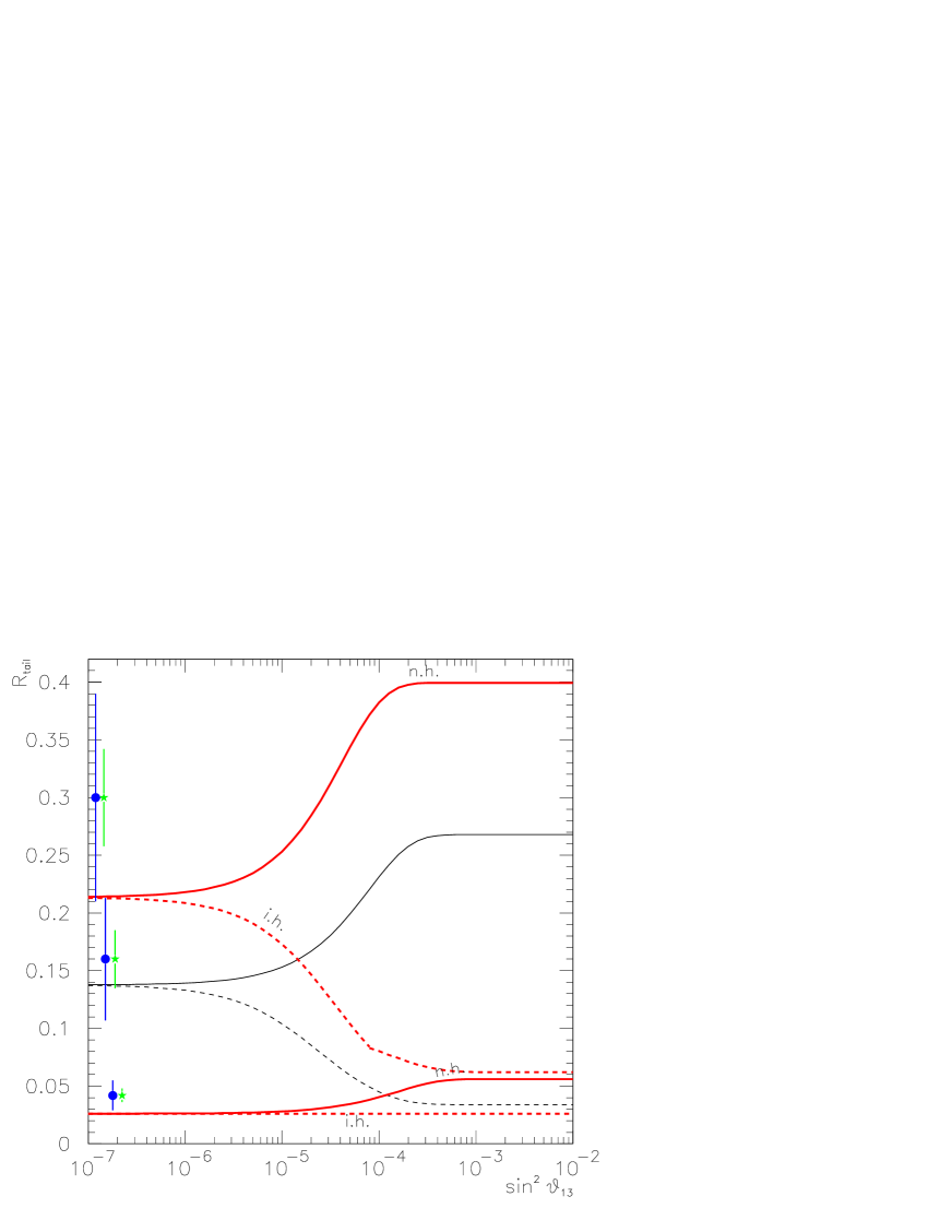
Figure 11: The same as fig. 10 for Earth crossing trajectories. We took $\Delta m^{2}_{21}=5\cdot 10^{-5}~{}{\rm eV^{2}}$ and the nadir angles $\theta_{n}=84.3^{\circ}$ at SNO and $\theta_{n}=24.5^{\circ}$ at SK.

Similarly to what discussed in secs. 6.5 and 6.6, using (110) we calculate the interval of possible values of $R_{tail}$, $R_{min}\div R_{max}$, taking into account all the uncertainties, including those on $f$ and $\bar{f}$. The results are shown in fig. 11. Notice that with respect to the no-crossing case, a stronger dependence of $R_{tail}$ on $\theta_{13}$ is seen for n.h., implying a larger sensitivity of the data to the normal mass hierarchy. This is related to the fact that the Earth regeneration effect is stronger in the $\mathrel{{\nu_{e}}}$ than in the $\mathrel{{\bar{\nu}}_{e}}$ channel.

Let us mark that the observation of oscillatory distortions due to Earth matter effects in the energy spectrum of the $\mathrel{{\nu_{e}}}$ ($\mathrel{{\bar{\nu}}_{e}}$) signal can establish the normal (inverted) mass hierarchy [5, 65] Once the information on the hierarchy is known, the method discussed here will provide a measurement or bound on $\theta_{13}$.

6.8 Refining the method

As we saw in the previous sections appearance of the $\alpha$-terms substantially reduces the identification power of the method (cf. fig 9 and 10). Let us consider the possibilities to refine it.

1. Further studies of the physics of supernovae can lead to more precise predictions for the original neutrino spectra. Furthermore, one can use results of studies of the whole neutrino and antineutrino spectra to reduce the uncertainty intervals of the average energies and fluxes, which then can be used in the tail method.

2. One can take larger cut energies $E_{L}$ and $\bar{E}_{L}$. With the increase of $E_{L}$ and $\bar{E}_{L}$ the $\alpha$-terms decrease and the picture shown in fig. 9 will approach that in fig. 8. For higher $E_{L}$ and $\bar{E}_{L}$ the hierarchy can be identified in a larger interval of $r$ (and $R_{tail}$) and the 13-mixing can be measured (especially in the case of inverted hierarchy). This will be possible in the case the distance to the supernova is relatively small, so that the statistics is high enough.

3. One can determine $\alpha$, $\bar{\alpha}$ or other relevant parameters of the original neutrino spectra immediately from the experimental data. This can be done by studying the dependences of the numbers of events $N_{e}(E_{L})$, $N_{\bar{e}}(\bar{E}_{L})$, as well as their ratio $R_{tail}$, on the threshold energies $E_{L}$, $\bar{E}_{L}$. Indeed, the number of events $N_{e}(E_{L})$ depends on $E_{L}$ via the quantities $N^{0}_{x}$ and $\alpha$:

$$N_{e}(E_{L})=(1-p)N_{x}^{0}(E_{L})(1-p+p\alpha(E_{L}))~{}.$$ (112)

These two contributions in principle can be disentangled, since they are different functions of $E_{L}$. As follows from eq. (70), $\alpha$ has an exponential dependence on $E_{L}$ of the form: $\alpha(E_{L})=A\exp(-E_{L}/T_{ex})$ (with $1/T_{ex}\equiv 1/T_{e}-1/T_{x}$). A fit of data could provide the unknown parameters $A$ and $T_{ex}$, allowing to fully reconstruct the function $\alpha(E_{L})$.

7 Time dependence of the signal: shock-wave effects

7.1 Shock wave and H-resonance

As it was pointed out in ref. [33], the shock-wave propagating inside the star may reach the region of densities relevant for neutrino conversion during the neutrino emission period ($10-20$ seconds). It modifies the density profile of the star, thus affecting the pattern of neutrino conversion [33, 69].

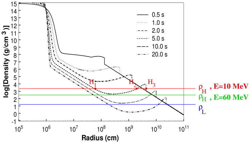
Figure 12: The density profile at various times post-bounce as adopted in ref. [33]. The horizontal lines represent the resonance densities $\rho_{H}$ (for two values of the neutrino energy) and $\rho_{L}$; the three high-density resonances $H_{1},H_{2},H_{3}$ are marked for $t=5$ s and $E=10$ MeV.

An indicative description of the time dependence of the matter density profile is given in fig. 12 (adapted from [33]). As shown in the figure, at a given time $t$ post-bounce, the density distribution presents an overdense region corresponding to the shock-front. The outer border of this region (front) consists in a sharp “step” in which the density increases from $\rho_{i}$ to $\rho_{f}$. According to [33] the relative increase of the density in the front, $\xi$, can be of about an order of magnitude:

$$\xi\equiv\rho_{f}/\rho_{i}\sim 10.$$ (113)

Above the shock front the profile coincides with that of the progenitor star. Below the front a rarefaction region, a “hot bubble”, is produced.

According to [33], the velocity of the shock front, $v_{s}$, increases with the distance from the center of the star. For distances $d=(1-5)\cdot 10^{3}$ km it changes in the interval

$$v_{s}\sim(0.8-1.2)\cdot 10^{4}~{}{\rm Km/s},$$ (114)

and for $d>5\cdot 10^{3}$ km, $v_{s}$ is nearly constant: $v_{s}\approx 1.2\cdot 10^{4}~{}{\rm Km/s}$.

The shock wave influences the neutrino conversion when it reaches the resonance layer. Given the mass squared splitting $\Delta m^{2}$, the neutrino level crossing (resonance) is realized at the density

$$\rho_{res}=\frac{m_{N}\Delta m^{2}}{\sqrt{2}G_{F}E}\cos 2\theta_{13}\simeq 1.4\cdot 10^{3}{\rm g\cdot cm^{-3}}\left(\frac{\Delta m^{2}}{10^{-3}~{}{\rm eV^{2}}}\right)\left(\frac{10~{}{\rm MeV}}{E}\right),$$ (115)

where $m_{N}$ is the nucleon mass and $G_{F}$ the Fermi constant and we have taken the electron fraction $Y_{e}=1/2$. From the fig. (12) and eq. (7) we find the resonance radius :

$$d_{res}=5\cdot 10^{4}{\rm km}\left(\frac{10^{-3}~{}{\rm eV^{2}}}{\Delta m^{2}}\right)^{1/3}\left(\frac{E}{10~{}{\rm MeV}}\right)^{1/3}~{},$$ (116)

and – taking a constant speed $v_{s}$ with values (114) – one gets the time $t_{s}\sim d_{res}/v_{s}$ after which the shockwave reaches the resonance:

$$t_{s}(E)=\frac{d_{res}}{v_{s}}=(4-5)~{}{\rm s}\left(\frac{E}{10~{}{\rm MeV}}\right)^{1\over 3}~{}.$$ (117)

For the H resonance ($\Delta m^{2}\simeq 3\cdot 10^{-3}~{}{\rm eV^{2}}$) and $E=10$ MeV we have $\rho_{res}\simeq 4000~{}{\rm g\cdot cm^{-3}}$, $d_{res}\simeq 5\cdot 10^{4}$ Km (see fig. 12) and $t_{s}\simeq 5$ s. The period $\Delta t_{s}$ during which the H resonance is on the shock front (i.e. $\rho_{i}\leq\rho_{res}\leq\rho_{f}$) can be estimated as the time which the shock wave takes to propagate from the position of the resonance, $d_{res}$ ($\rho_{i}=\rho_{res}$) to the position $d_{f}$ at which $\rho_{f}=\rho_{res}$. The latter can be found using the density profile (7):

$$d_{f}=d_{res}\xi^{1/3}~{}.$$ (118)

Then the interval $\Delta t_{s}$ equals:

$$\Delta t_{s}=\frac{d_{res}}{v_{s}}(\xi^{1/3}-1).$$ (119)

Taking $\xi\approx 10$ (eq. (113)) and constant velocity $v_{s}$, (114), we get

$$\Delta t_{s}\approx(5-6)~{}{\rm sec}\left(\frac{E}{10{\rm MeV}}\right)^{1/3}$$ (120)

which is comparable with the arrival time $t_{s}$.

According to eqs. (117) and (120), $t_{s}$ and $\Delta t_{s}$ increase with energy: for the lowest detectable energies in the spectrum one gets $t_{s}(6{\rm MeV})=3-5$ s, while for the highest energies $t_{s}(70{\rm MeV})=7-10$ s is obtained.

Let us mark, however, that the details of the shock-wave propagation depend on the specific characteristics of the progenitor and therefore even large variations of parameters are expected between different SN models.

Let us consider the conversion in the H resonance and its modifications due to the passage of the shock wave. For a given neutrino energy three time intervals can be defined:

1. The pre-shock phase, $t(E)\mathrel{\vbox{\hbox{$<$}\nointerlineskip\hbox{$\sim$}}}t_{s}(E)\sim 3-5$ sec, in which the shock has not yet reached the resonance region and therefore has no effects on the neutrino conversion.

2. The shock phase, $t(E)=t_{s}(E)-(t_{s}(E)+\Delta t_{s}(E))$, when the resonance condition $\rho=\rho_{res}$ is fulfilled in the step of the shock front.

As it follows from the fig. 12, in this phase three resonances appear at three different radii: two of them are on the walls of the hot bubble, while the third is at the shock front. We denote these resonances as $H_{1},H_{2},H_{3}$ from the inner to the outer.

For a given value of $\mathrel{{\sin^{2}\theta_{13}}}$, the conversion pattern due to the presence of these resonances exhibits a variety of possibile scenarios, depending on the adiabaticity character of these resonances, and therefore on the details of the density profile of the bubble and of the shock front. The shock-wave propagation has no effect if $\mathrel{{\sin^{2}\theta_{13}}}\mathrel{\vbox{\hbox{$<$}\nointerlineskip\hbox{$\sim$}}}10^{-6}$, corresponding to non–adiabatic neutrino conversion in all the relevant resonances during both the pre-shock and the shock phases. Therefore in what follows we discuss the case in which $\mathrel{{\sin^{2}\theta_{13}}}$ is in the adiabatic region of the H resonance in the pre-shock regime, that is, $\mathrel{{\sin^{2}\theta_{13}}}\mathrel{\vbox{\hbox{$>$}\nointerlineskip\hbox{$\sim$}}}10^{-4}$ (see fig. 1), and the $H_{1}$ and $H_{2}$ resonances are adiabatic, while the adiabaticity is broken in the $H_{3}$ resonance. In this case the permutation parameters $p$ (for n.h.) and $\bar{p}$ (for i.h. ) are given by eqs. (20)-(23) with $P_{H}$ being the jumping probability in the $H_{3}$ resonance. For maximal adiabaticity breaking

$$P_{H}\approx P_{H_{3}}\sim 1~{}.$$ (121)

The effect of the arrival of the shock-wave consists in a sudden change of the character of the H level crossing from adiabatic to maximally non–adiabatic, with significant modifications of the observed neutrino signal.

3. The post-shock phase, $t(E)>t_{s}(E)+\Delta t_{s}(E)$, when the matter density at the shock front is smaller than the resonance density $\rho_{res}\geq\rho_{f}$, so that only one level crossing, $H_{1}$, survives. The conversion effects are described by the transition probability in the $H_{1}$ resonance: $P_{H}\simeq P_{H_{1}}\sim 0$. In the transition between the shock and the post-shock phases, the resonance points $H_{2}$ and $H_{3}$ become closer until they merge and disappear .

For the scenario discussed here we expect the following time dependence of the effective jumping probability $P_{H}$:

$$P_{H}\approx\begin{cases}0&\text{for}~{}~{}t\mathrel{\vbox{\hbox{$<$}\nointerlineskip\hbox{$\sim$}}}t_{s}(E)\\ 1&\text{for}~{}~{}t=t_{s}(E)-(t_{s}+\Delta t_{s}(E))\\ 0&\text{for}~{}~{}t\mathrel{\vbox{\hbox{$>$}\nointerlineskip\hbox{$\sim$}}}t_{s}(E)+\Delta t_{s}(E)~{}.\end{cases}$$ (122)

In general, the shock wave effect is proportional to $P_{H_{3}}$, which in turn depends on the neutrino energy. Therefore not only the time but also the size of the effect depend on the energy. The ratio of the adiabaticity parameters of a resonance at and above the shock front (where the density profile equals that of the progenitor star) equals the ratio of the corresponding density gradients:

$$\frac{\gamma_{f}}{\gamma_{i}}\equiv k_{grad}=\frac{(d\rho/dr)_{f}}{(d\rho/dr)_{0}}~{}.$$ (123)

From this and eqs. (13,14) it follows that for $\sin^{2}\theta_{13}=0.01$ the adiabaticity is violated at all relevant energies if $k_{grad}=10^{4}$. That is the gradient of density in the shock wave is 4 orders of magnitude larger than the gradient of the progenitor profile (at the same density). If $k_{grad}=10^{3}$, we get $P_{H_{3}}\approx 1$ for high energies: $E\sim 70$ MeV but $P_{H_{3}}\sim 0.5$ for $E\sim 6$ MeV. For smaller gradient: $k_{grad}=10^{2}$, the adiabaticity is not violated for low energies, and therefore there is no shock wave effect, but it is still violated for high energies: $P_{H_{3}}\sim 0.5$ for $E\sim 70$ MeV. In general one expects larger effects for high energies. Results for other values of $\sin^{2}\theta_{13}$ can be obtained immediately by rescaling eqs. (13,14).

7.2 Shock wave effects on the neutrino spectra

Let us consider the influence of the shock wave on the neutrino spectra in more details. For a given energy $E$ the effect of the shock wave consists in a change of the flux when the front of shock wave reaches the corresponding resonance layer with resonance density $\rho_{res}(E)$ and then restoration of the original (undisturbed) flux after the front shock shifts to smaller densities. In what follows for simplicity we will assume that the density gradient in the shock wave is large enough so that the adiabaticity is strongly broken for all observable energies.

In the case of normal mass hierarchy (H-resonance in the neutrino channel) during the interval $\Delta t_{s}$ the shock wave leads to a change of the $\mathrel{{\nu_{e}}}$ flux exiting the star from completely to partially permuted:

$$F_{x}^{0}(E)\rightarrow F_{s}(E)=\cos^{2}\theta_{12}F_{x}^{0}(E)+\sin^{2}\theta_{12}F_{e}^{0}(E).$$ (124)

Let us introduce critical energy $E_{c}$ such that $F_{x}^{0}(E_{c})=F_{e}^{0}(E_{c})$. Then for $E<E_{c}$ we have $F^{0}_{x}(E)<F_{s}(E)$, and for $E>E_{c}$ the inequality $F^{0}_{x}(E)>F_{s}(E)$ holds. So, the pattern of perturbation of the whole spectrum can be described as follows: first the perturbation reaches the lowest energies of the spectrum and then propagates to high energies. We can say that the wave of perturbation of the spectrum propagates in the energy scale. It leads to an increase of the flux of the electron neutrinos according to eq. (124) when the wave propagates up to $E_{c}$. Then for $E>E_{c}$ the pertubation decreases the flux according to (124). So, we can say that the shock-wave effects consist in a wave of softening of the spectrum which propagates from low to high energies (softening wave). When the wave reaches the highest energies of spectrum, the perturbation start to disappear at low energies, restoring the original spectrum:

$$F_{s}(E)\rightarrow F^{0}_{x}(E)~{}.$$ (125)

The spectrum becomes hard again and the restoration moves again from low to high energies.

The antineutrino conversion will not be affected by the shock wave.

In the case of inverted mass hierarchy the H-resonance is in the antineutrino channel and therefore the shock wave will modify the antineutrino conversion. Similarly to (124) $\bar{\nu}_{e}$ spectrum changes as

$$F_{\bar{x}}^{0}(E)\leftrightarrow F_{\bar{s}}(E)=\sin^{2}\theta_{12}F_{\bar{x}}^{0}(E)+\cos^{2}\theta_{12}F_{\bar{e}}^{0}(E).$$ (126)

Although now the change of the permutation factor is stronger (from complete permutation to weak permutation: $(1-\bar{p})=1\leftrightarrow\sin^{2}\theta_{12}$), the effect on the spectrum can be similar to the normal hierarchy case due to the smaller difference of $F_{\bar{x}}^{0}(E)$ and $F_{\bar{e}}^{0}(E)$ fluxes. The neutrino flux will not be affected by the shock wave.

7.3 Shock wave and the Earth matter effect

The shock wave propagation can influence the Earth matter effect. Indeed, for the normal mass hierarchy the Earth matter effect in $\mathrel{{\nu_{e}}}$ channel vanishes for adiabatic H transition while it is maximal for maximal violation of the adiabaticity in the H resonance, $P_{H}=1$ [5, 65]. The effect increases fast with energy, reaching 30 - 50 % at $E\sim 50-70$ MeV.

Taking this into account, for the scenario (122) we get the following time dependence:

in the pre-shock phase, no regeneration effect is realized in the $\mathrel{{\nu_{e}}}$ channel due to the adiabaticity character of the H resonance. The effect is small in the first few seconds of the shock wave phase: in this interval the adiabaticity is broken at low energies, where the Earth matter effect is small. After 5 - 7 sec the softening wave reaches the high energy region, where the Earth matter effect is large. So one expects the absence of the Earth matter effects in the first 5 - 7 sec of the neutrino burst and then its fast increase with time in the high energy part of the spectrum. We will call this the delayed Earth matter effect.

Being unaffected by the H resonance, the $\mathrel{{\bar{\nu}}_{e}}$ spectrum exhibits the Earth matter effects for the whole duration of the neutrino signal.

In contrast, if the mass hierarchy is inverted, the Earth matter effect is observed in the neutrino channel during the whole burst and it appears in the antineutrino channel in the late stage (after 5 - 7 sec).

7.4 Shock wave effects, mass hierarchy and $\theta_{13}$

Precise measurements of the energy spectra in different moments of time can, in principle, reveal spectrum distortions which depend on time and propagate from low to high energies. For this however very high statistics is needed.

Another possibility is to use some global characteristics of spectra and their change with time to look for shock wave effects. In particular, one expects

• decrease of the average energy of the spectrum $\langle E\rangle$ which reflects its softening during the shock wave phase;

• increase of the relative width $\Gamma$, as a consequence of the appearance of a composite spectrum during the time $\Delta t_{s}$;

• appearance of the Earth matter effect in the late stage of the burst;

• change in the total even rates [33].

A problem of dealing with global characteristics is the possible degeneracy between the changes of the neutrino energy spectra due to shock wave effects and those due to astrophysical factors (cooling of the energy spectra, decay of the luminosity, etc.).

The shock-wave effects on the $\mathrel{{\nu_{e}}}$ (or $\mathrel{{\bar{\nu}}_{e}}$) signal could be identified by studying the time dependence of the ratios of $\mathrel{{\nu_{e}}}$ (for n.h.) or $\mathrel{{\bar{\nu}}_{e}}$ (for i.h.) CC to NC event rates at SNO [33]. Since the NC rate is not affected by shock-induced conversion effects, the CC to NC ratio represents a particularly “clean” quantity, in which various time-dependent features other than the shock effect (e.g. cooling of energy spectra) are at least partially subtracted. Using this method, in ref. [33] it is found that the distortion due to the shock-wave amounts to $\sim 30\%$, whose statistical significance has not been clarified, however.

An alternative approach to probe effects of the passage of the shock wave could be to study the time dependence of the ratio $R_{tot}$ of the total number of $\mathrel{{\nu_{e}}}$ and $\mathrel{{\bar{\nu}}_{e}}$ events (eq. (58)), where still an at least partial subtraction of cooling effects is realized. In this quantity the uncertainties related to the poor knowledge of astrophysical parameters can by no means mimic a specific time structure and therefore should be distinguishable from the shock effects.

The observation of the delayed Earth matter effect is another signature of the shock wave effects.

Let us summarize the possibilities to identify the mass hierarchy and measure (or restrict) $\theta_{13}$.

The observation of shock-effects in $\mathrel{{\nu_{e}}}$ ($\mathrel{{\bar{\nu}}_{e}}$) channel would select the normal (inverted) mass hierarchy and would tell that $\mathrel{{\sin^{2}\theta_{13}}}$ is relatively large, $\mathrel{{\sin^{2}\theta_{13}}}\mathrel{\vbox{\hbox{$>$}\nointerlineskip\hbox{$\sim$}}}5\cdot 10^{-4}$, so that $P_{H}<1$ significantly in the pre-shock phase. Moreover, it would allow to study the physical features of the shock-propagation (speed, etc.). The exclusion of shock-effects would imply that $\mathrel{{\sin^{2}\theta_{13}}}$ is in the adiabaticity breaking region in the pre-shock times or that the properties of the shock wave differ significantly from the predictions (e.g. that the shock stalls, or travels with smaller velocity, so that the shock does not reach the resonance region during the duration of the burst, or that the shock front is not steep enough to change the adiabaticity character of the conversion).

Quantitative estimates of the bounds on $\mathrel{{\sin^{2}\theta_{13}}}$ that can be obtained from the study of shock-induced time dependences of the signal will be given elsewhere [70].

8 Discussion and conclusions

I. We have studied the effects of the 13-mixing on the conversion of the supernova neutrinos.

If $\theta_{13}$ is negligible ($\mathrel{{\sin^{2}\theta_{13}}}\mathrel{\vbox{\hbox{$<$}\nointerlineskip\hbox{$\sim$}}}10^{-5}$), at the cooling stage a partial permutation of the original $\mathrel{{\nu_{e}}}$ and $\mathrel{{\nu_{x}}}$, $\mathrel{{\bar{\nu}}_{e}}$ and $\mathrel{{\bar{\nu}}_{x}}$ energy spectra occurs in the star due to the large 12-mixing. For larger values of $\theta_{13}$, $\sin^{2}\theta_{13}\geq 10^{-5}$, these conversion effects are modified in the $\mathrel{{\nu_{e}}}$ ($\mathrel{{\bar{\nu}}_{e}}$) channel for normal (inverted ) mass hierarchy.

For normal mass hierarchy the degree of permutation in $\mathrel{{\nu_{e}}}$ channel increases from $(1-p)=\cos^{2}\theta_{12}\sim 0.7-0.8$ to $(1-p)=\cos^{2}\theta_{12}+(1-P_{H})\sin^{2}\theta_{12}$, resulting in an hardening of the observed $\mathrel{{\nu_{e}}}$ spectrum. If $\sin^{2}\theta_{13}>10^{-4}$ the transition driven by $\theta_{13}$ is adiabatic and the change is maximal: $(1-p)\approx 1$. This corresponds to a complete permutation and therefore maximally hard $\mathrel{{\nu_{e}}}$ spectrum.

Some additional distortion of the energy spectrum is expected for $\sin^{2}\theta_{13}<10^{-4}$ due to the dependence of the jumping probability $P_{H}$ on energy.

In the case of inverted mass hierarchy the 13 mixing leads to an increase of the degree of permutation in the antineutrino channel: from $(1-\bar{p})=\sin^{2}\theta_{12}$ to $(1-\bar{p})=\sin^{2}\theta_{12}+(1-P_{H})\cos^{2}\theta_{12}$. Again for $\sin^{2}\theta_{13}>10^{-4}$ the effect is maximal: $(1-\bar{p})\approx 1$.

In this paper we have elaborated methods to study the effects of the $\theta_{13}$ mixing in presence and absence of Earth matter effects. Various possibilities to probe the mass hierarchy and measure (or restrict) $\theta_{13}$ have been discussed as well.

II. The permutation due to $\theta_{13}$ changes the average energy and width of the $\mathrel{{\nu_{e}}}$ (for n.h.) or $\mathrel{{\bar{\nu}}_{e}}$ (for i.h.) spectrum. Signatures of these modifications can be obtained from the comparison of the features of neutrino and antineutrino spectra.

In particular, for large 13-mixing and the normal mass hierarchy one expects $\langle E(\nu)\rangle>\langle E(\bar{\nu})\rangle$ and $\langle\Gamma(\nu)\rangle<\langle\Gamma(\bar{\nu})\rangle$. Opposite inequalities are expected in the case of inverted hierarchy.

In this connection we have studied the observed spectra of events from $\mathrel{{\nu_{e}}}+d$ and $\mathrel{{\bar{\nu}}_{e}}+p$ CC reactions at SNO and SK respectively; in particular, the following observables have been considered: the ratio of the average energies of the $\mathrel{{\nu_{e}}}$ and $\mathrel{{\bar{\nu}}_{e}}$ events, $r_{E}=\langle E\rangle/\langle\bar{E}\rangle$, the ratio of the widths of the energy spectra, $r_{\Gamma}=\Gamma/{\bar{\Gamma}}$, and the ratio $R_{tail}$ of the numbers of events in the high energy tails (above certain energy cuts $E_{L}$ and $\bar{E}_{L}$) at the two experiments. These quantities depend on $\theta_{13}$ via the jumping probability in the H resonance, $P_{H}(\theta_{13})$.

Although the 13-mixing produces a strong conversion, the corresponding observable effects may not be so large due to presence of neutrino fluxes of all types and also due to effects of the 12-mixing effect (see item I ). Furthermore, substantial astrophysical uncertainties make the identification of the 13-mixing effects difficult, due to possible degeneracies between the parameters of the original neutrino spectra and the oscillation parameters.

We have studied the effects of uncertainties on: (i) the energy spectra and luminosities of the neutrino fluxes originally produced inside the star, (ii) the density profile of the star, (iii) the mass square splitting $\Delta m^{2}_{31}$, (iii) the mixing angle $\theta_{12}$.
Methods to take these uncertainties into account in the data analysis have been elaborated.

III. We have considered the cases of adiabatic transition ($P_{H}=0$) with (A) of normal mass hierarchy and (B) inverted mass hierarchy and we have compared them with the case (C) of maximally non-adiabatic conversion (i.e. negligibly small $\theta_{13}$: $\sin^{2}\theta_{13}<10^{-5}$).

The scatter plots of the observables ($r_{E}$, $r_{\Gamma}$, $R_{tail}$,…) for these three cases show that there are regions – in the space of these parameters – where only one or two possibilities exists, implying the exclusion of the remaining ones.

In particular,

• The case A is excluded if observations give $R_{tail}\mathrel{\vbox{\hbox{$<$}\nointerlineskip\hbox{$\sim$}}}0.06$ and/or $r_{\Gamma}\mathrel{\vbox{\hbox{$>$}\nointerlineskip\hbox{$\sim$}}}1.1$. If, in contrast, the experiments give $R_{tail}>0.22$ the normal hierarchy would be identified. This result would be further supported if $r_{\Gamma}\mathrel{\vbox{\hbox{$<$}\nointerlineskip\hbox{$\sim$}}}0.9$ is also found.

• The case B is excluded by (i) large values of $R_{tail}$, $R_{tail}\mathrel{\vbox{\hbox{$>$}\nointerlineskip\hbox{$\sim$}}}0.07$, (ii) large values of the ratio of average energies $r_{E}\mathrel{\vbox{\hbox{$>$}\nointerlineskip\hbox{$\sim$}}}1.2$ and (iii) $r_{\Gamma}\mathrel{\vbox{\hbox{$<$}\nointerlineskip\hbox{$\sim$}}}1$. In contrast, the identification of this scenario appears difficult.

• The case C is difficult to single out. The result $r_{\Gamma}\mathrel{\vbox{\hbox{$>$}\nointerlineskip\hbox{$\sim$}}}1.1$ and $0.06\mathrel{\vbox{\hbox{$<$}\nointerlineskip\hbox{$\sim$}}}R_{tail}\mathrel{\vbox{\hbox{$<$}\nointerlineskip\hbox{$\sim$}}}0.2$ would exclude B and A, and therefore indicate that $P_{H}>0$, corresponding to small values of $\theta_{13}$: $\mathrel{{\sin^{2}\theta_{13}}}\mathrel{\vbox{\hbox{$<$}\nointerlineskip\hbox{$\sim$}}}few\cdot 10^{-4}$.

IV. The high energy tail method allows, in principle, to establish the mass hierarchy and to restrict or to measure $\sin^{2}\theta_{13}$. Taking the thresholds $E_{L}=45$ MeV and $\bar{E}_{L}=55$ MeV and $\mathrel{{\tan^{2}\theta_{12}}}=0.38$ as an example, we find that if $R>0.22$ the normal mass hierarchy can be identified and a lower bound on $\sin^{2}\theta_{13}$ can be obtained. For smaller values of the mixing the hierarchy can not be established; however strong bounds on $\sin^{2}\theta_{13}$ are put if the mass hierarchy is know from other results (e.g. by measurements of other parameters of spectra, by studying the Earth regeneration effects etc.). A measurement of $\theta_{13}$ will be possible only if a reduction of the uncertainties on the original neutrino fluxes is achieved.

The Earth matter effect enhances the identification power of the method. Since the regeneration is larger in neutrino than in antineutrino channel, the sensitivity of $R_{tail}$ to the n.h. (i.h.) is enhanced (reduced) with respect to the no Earth-crossing case. In particular, in presence of Earth effects the method of analysis discussed in this paper would be complementary to the information that can be extracted from the observation of oscillatory distortions in the energy spectra of $\mathrel{{\nu_{e}}}$ and/or $\mathrel{{\bar{\nu}}_{e}}$ events in the detectors.

The method of the high energy tails can be improved if (i) additional information about parameters of the neutrino fluxes is obtained from the studies of the whole spectra (and not only of the high energy tails) (ii) if the dependence of the ratio $R_{tail}$ on the energy cuts is studied, (iii) higher energy cuts are used. These improvements can be implemented if the statistics is large enough.

V. The study of shock-wave effects on the neutrino burst, which can be realized at late times ($t\mathrel{\vbox{\hbox{$>$}\nointerlineskip\hbox{$\sim$}}}5$ s) could provide additional information on the $\theta_{13}$ angle and the mass hierarchy (in support of the methods discussed in sections 5. and 6., which refers to early times, $t\mathrel{\vbox{\hbox{$<$}\nointerlineskip\hbox{$\sim$}}}5$ s). In particular, the presence of time dependent spectral distortions produced by the shock-wave passage through the resonance layers would lead to the lower bound $\mathrel{{\sin^{2}\theta_{13}}}\mathrel{\vbox{\hbox{$>$}\nointerlineskip\hbox{$\sim$}}}few\cdot 10^{-4}$ and establish the n.h. (i.h.) if observed in the $\mathrel{{\nu_{e}}}$ ($\mathrel{{\bar{\nu}}_{e}}$) channel.

An important signature of the shock wave is the appearance of the delayed Earth matter effect in the neutrino or antineutrino channel at the late stages of the burst ($t>5-7$ sec). The channel of appearance will identify the mass hierarchy.

Acknowledgements

C.L. acknowledges support from the Keck fellowship and the grants PHY-0070928 and PHY99-07949. She would like to thank J. N. Bahcall, A. Friedland, C. Peña–Garay and H. Minakata for fruitful discussions, T. Totani for useful communications and the Kavli Institute of Theoretical Physics (KITP), Santa Barbara (CA), as hosting institution where part of this work was prepared. The authors are grateful to S. Palomares-Ruiz, O. L. G. Peres and F. Vissani for useful comments on the preliminary version of this paper.

Figure 2: The survival probabilities $p$ for n.h. (upper panel) and $\bar{p}$ for i.h. (lower panel) as functions of $\mathrel{{\sin^{2}\theta_{13}}}$ for $\tan^{2}\theta_{12}=0.38$ and different values of the neutrino energy. Other parameters as in fig. 1. The shaded region in the lower panel represents the error bar associated to a measurement $\bar{p}=0$. The corresponding lower bound on $\mathrel{{\sin^{2}\theta_{13}}}$, $\mathrel{{\sin^{2}\theta_{13}}}\mathrel{\vbox{\hbox{$>$}\nointerlineskip\hbox{$\sim$}}}2\cdot 10^{-4}$, is small enough to be calculated in the zeroth order approximation (i.e. neglecting the explicit $\mathrel{{\sin^{2}\theta_{13}}}$ dependence in eq. (23)). The error bar is much larger for the neutrino channel and normal hierarchy and was not drawn.

References

- [1] See e.g. the review: G. G. Raffelt, Physics with supernovae, Nucl. Phys. Proc. Suppl. 110 (2002) 254–267, [hep-ph/0201099], and references therein.
- [2] S. P. Mikheev and A. Y. Smirnov, Neutrino oscillations in a variable-density medium and neutrino bursts due to the gravitational collapse of stars, Sov. Phys. JETP 64 (1986) 4–7.
- [3] L. Wolfenstein, Effects of matter oscillations on supernova neutrino flux, Phys. Lett. B194 (1987) 197.
- [4] G. Dutta, D. Indumathi, M. V. N. Murthy, and G. Rajasekaran, Neutrinos from stellar collapse: effects of flavour mixing, Phys. Rev. D61 (2000) 013009, [hep-ph/9907372].
- [5] A. S. Dighe and A. Y. Smirnov, Identifying the neutrino mass spectrum from the neutrino burst from a supernova, Phys. Rev. D62 (2000) 033007, [hep-ph/9907423].
- [6] G. Dutta, D. Indumathi, M. V. N. Murthy, and G. Rajasekaran, Neutrinos from stellar collapse: comparison of the effects of three and four flavor mixings, Phys. Rev. D62 (2000) 093014, [hep-ph/0006171].
- [7] G. Dutta, D. Indumathi, M. V. N. Murthy, and G. Rajasekaran, Neutrinos from stellar collapse: comparison of signatures in water and heavy water detectors, Phys. Rev. D64 (2001) 073011, [hep-ph/0101093].
- [8] K. Takahashi, M. Watanabe, K. Sato, and T. Totani, Effects of neutrino oscillation on the supernova neutrino spectrum, Phys. Rev. D64 (2001) 093004, [hep-ph/0105204].
- [9] G. L. Fogli, E. Lisi, D. Montanino, and A. Palazzo, Supernova neutrino oscillations: a simple analytical approach, Phys. Rev. D65 (2002) 073008, [hep-ph/0111199].
- [10] V. Barger, D. Marfatia, and B. P. Wood, Inverting a supernova: neutrino mixing, temperatures and binding energy, Phys. Lett. B547 (2002) 37–42, [hep-ph/0112125].
- [11] H. Minakata, H. Nunokawa, R. Tomas, and J. W. F. Valle, Probing supernova physics with neutrino oscillations, Phys. Lett. B542 (2002) 239–244, [hep-ph/0112160].
- [12] V. Barger, D. Marfatia, and B. P. Wood, Supernova 1987A did not test the neutrino mass hierarchy, hep-ph/0202158.
- [13] K. Takahashi and K. Sato, Effects of neutrino oscillation on supernova neutrino: inverted mass hierarchy, hep-ph/0205070.
- [14] KamLAND Collaboration, K. Eguchi et. al., First results from KamLand: Evidence for reactor anti- neutrino disappearance, Phys. Rev. Lett. 90 (2003) 021802, [hep-ex/0212021].
- [15] V. D. Barger, D. Marfatia, and B. P. Wood, Resolving the solar neutrino problem with KamLand, Phys. Lett. B498 (2001) 53–61, [hep-ph/0011251].
- [16] R. Barbieri and A. Strumia, Non standard analysis of the solar neutrino anomaly, JHEP 12 (2000) 016, [hep-ph/0011307].
- [17] H. Murayama and A. Pierce, Energy spectra of reactor neutrinos at KamLand, Phys. Rev. D65 (2002) 013012, [hep-ph/0012075].
- [18] J. Arafune, M. Fukugita, T. Yanagida, and M. Yoshimura, Neutrino mass and mixing constrained from the LMC supernova burst, Phys. Lett. B194 (1987) 477.
- [19] T. P. Walker and D. N. Schramm, Resonant neutrino oscillations and the neutrino signature of supernovae, Phys. Lett. B195 (1987) 331.
- [20] D. Notzold, MSW effect analysis for SN1987A sets severe restrictions on neutrino masses and mixing angles, Phys. Lett. B196 (1987) 315–320.
- [21] H. Minakata and H. Nunokawa, Neutrino flavor conversion in supernova SN1987A, Phys. Rev. D38 (1988) 3605.
- [22] B. Jegerlehner, F. Neubig, and G. Raffelt, Neutrino oscillations and the supernova 1987A signal, Phys. Rev. D54 (1996) 1194–1203, [astro-ph/9601111].
- [23] C. Lunardini and A. Y. Smirnov, Neutrinos from SN1987A, earth matter effects and the LMA solution of the solar neutrino problem, Phys. Rev. D63 (2001) 073009, [hep-ph/0009356].
- [24] H. Minakata and H. Nunokawa, Inverted hierarchy of neutrino masses disfavored by supernova 1987A, Phys. Lett. B504 (2001) 301–308, [hep-ph/0010240].
- [25] M. Kachelriess, R. Tomas, and J. W. F. Valle, Large lepton mixing and supernova 1987A, JHEP 01 (2001) 030, [hep-ph/0012134].
- [26] M. Kachelriess, A. Strumia, R. Tomas, and J. W. F. Valle, SN1987A and the status of oscillation solutions to the solar neutrino problem, hep-ph/0108100.
- [27] See e.g. M. T. Keil, G. G. Raffelt, and H.-T. Janka, Monte carlo study of supernova neutrino spectra formation, astro-ph/0208035, and references therein.
- [28] C. J. Horowitz, Weak magnetism for antineutrinos in supernovae, Phys. Rev. D65 (2002) 043001, [astro-ph/0109209].
- [29] H. T. Janka and W. Hillebrandt, Monte Carlo simulations of neutrino transport in type II supernovae, Astron. Astroph. Suppl. 78 (1989) 375; H. T. Janka and W. Hillebrandt, Neutrino emission from type II supernovae - an analysis of the spectra, Astron. Astrophys. 224 (1989) 49.
- [30] See also G. G. Raffelt, “Stars as laboratories for fundamental physics: The astrophysics of neutrinos, axions, and other weakly interacting particles,” Chicago, USA: Univ. Pr. (1996) 664 p.
- [31] G. E. Brown, H. A. Bethe and G. Baym, Nucl. Phys. A 375 (1982) 481.
- [32] T. K. Kuo and J. Pantaleone, Supernova neutrinos and their oscillations, Phys. Rev. D37 (1988) 298.
- [33] R. C. Schirato and G. M. Fuller, Connection between supernova shocks, flavor transformation, and the neutrino signal, astro-ph/0205390.
- [34] P. I. Krastev and S. T. Petcov, Resonance amplification and t violation effects in three neutrino oscillations in the earth, Phys. Lett. B205 (1988) 84–92.
- [35] Super-Kamiokande Collaboration, S. Fukuda et. al., Tau neutrinos favored over sterile neutrinos in atmospheric muon neutrino oscillations, Phys. Rev. Lett. 85 (2000) 3999–4003, [hep-ex/0009001].
- [36] G. L. Fogli et. al., Solar neutrino oscillation parameters after first KamLand results, hep-ph/0212127.
- [37] J. N. Bahcall, M. C. Gonzalez-Garcia, and C. Pena-Garay, Solar neutrinos before and after KamLand, hep-ph/0212147.
- [38] H. Nunokawa, W. J. Teves and R. Zukanovich Funchal, Determining the oscillation parameters by solar neutrinos and KamLand, hep-ph/0212202.
- [39] P. C. de Holanda and A. Y. Smirnov, LMA MSW solution of the solar neutrino problem and first KamLand results, hep-ph/0212270.
- [40] CHOOZ Collaboration, M. Apollonio et. al., Limits on neutrino oscillations from the Chooz experiment, Phys. Lett. B466 (1999) 415–430, [hep-ex/9907037].
- [41] F. Boehm et. al., Results from the Palo Verde neutrino oscillation experiment, Phys. Rev. D62 (2000) 072002, [hep-ex/0003022].
- [42] A. Friedland, On the evolution of the neutrino state inside the sun, Phys. Rev. D64 (2001) 013008, [hep-ph/0010231].
- [43] M. Kachelriess and R. Tomas, Non-adiabatic level crossing in (non-) resonant neutrino oscillations, Phys. Rev. D64 (2001) 073002, [hep-ph/0104021].
- [44] T. K. Kuo and J. Pantaleone, Neutrino oscillations in matter, Rev. Mod. Phys. 61 (1989) 937.
- [45] C. Lunardini and A.Yu. Smirnov, in preparation.
- [46] D. D. Clayton, “Principles of Stellar Evolution and Nucleosynthesis,” Chicago, USA: Univ. Pr. (1983) 612 p.
- [47] K. Shigeyama, T.; Nomoto, Theoretical light curve of SN1987A and mixing of hydrogen and nickel in the ejecta, Astrophys. J. 360 (1990) 242–256.
- [48] V. D. Barger et. al., Neutrino oscillation parameters from Minos, Icarus and Opera combined, Phys. Rev. D65 (2002) 053016, [hep-ph/0110393].
- [49] See e.g. M. Shiozawa, talk given at the “International Workshop on a Next Generation Long-Baseline Neutrino Oscillation Experiment”; transparecies available at http://neutrino.kek.jp/jhfnu/workshop2/ohp.html.
- [50] C. K. Jung, Feasibility of a next generation underground water cherenkov detector: UNO, hep-ex/0005046.
- [51] See also M.Vagins, talk given at the ”Conference on Underground Science”, Lead, South Dakota (USA), October 4-7, 2001, transparencies available at http://mocha.phys.washington.edu/int_talk/NUSL/2001/People?Vagins_M.
- [52] TITAND Working Group Collaboration, Y. Suzuki et. al., Multi-megaton water cherenkov detector for a proton decay search: Titand (former name: Titanic), hep-ex/0110005.
- [53] J. F. Beacom and P. Vogel, Mass signature of supernova nu/mu and nu/tau neutrinos in Superkamiokande, Phys. Rev. D58 (1998) 053010, [hep-ph/9802424].
- [54] J. F. Beacom and P. Vogel, Mass signature of supernova nu/mu and nu/tau neutrinos in the Sudbury neutrino observatory, Phys. Rev. D58 (1998) 093012, [hep-ph/9806311].
- [55] See e.g. C. Waltham, proceedings from the International Conference on Cosmic Rays (ICRC) 2001, available at www.copernicus.org/icrc/papers/ici7144_p.pdf .
- [56] M. Aglietta et al., Effects of neutrino oscillations on the supernova signal in LVD, Nucl. Phys. Proc. Suppl. 110, 410 (2002) [astro-ph/0112312].
- [57] F. Arneodo et al. [ICARUS collaboration], The ICARUS experiment, a second-generation proton decay experiment and neutrino observatory at the Gran Sasso Laboratory, hep-ex/0103008.
- [58] A. Strumia and F. Vissani, Massive Neutrinos And Theoretical Developments, Int. J. Mod. Phys. A 17, 1755 (2002).
- [59] D. B. Cline, F. Sergiampietri, J. G. Learned and K. McDonald, LANNDD: A massive liquid argon detector for proton decay, supernova and solar neutrino studies, and a neutrino factory detector, astro-ph/0105442.
- [60] S. Nakamura, T. Sato, V. Gudkov, and K. Kubodera, Neutrino reactions on deuteron, Phys. Rev. C63 (2001) 034617, [nucl-th/0009012].
- [61] P. Vogel and J. F. Beacom, The angular distribution of the reaction , Phys. Rev. D60 (1999) 053003, [hep-ph/9903554].
- [62] J. F. Beacom and S. J. Parke, On the normalization of the neutrino deuteron cross section, Phys. Rev. D64 (2001) 091302, [hep-ph/0106128].
- [63] A. Strumia and F. Vissani, Precise quasielastic neutrino nucleon cross section , astro-ph/0302055.
- [64] E. K. Akhmedov, C. Lunardini, and A. Y. Smirnov, Supernova neutrinos: Difference of nu/mu - nu/tau fluxes and conversion effects, Nucl. Phys. B643 (2002) 339–366, [hep-ph/0204091].
- [65] C. Lunardini and A. Y. Smirnov, Supernova neutrinos: Earth matter effects and neutrino mass spectrum, Nucl. Phys. B616 (2001) 307–348, [hep-ph/0106149].
- [66] K. Takahashi, M. Watanabe, and K. Sato, The earth effects on the supernova neutrino spectra, Phys. Lett. B510 (2001) 189–196, [hep-ph/0012354].
- [67] K. Takahashi and K. Sato, Earth effects on supernova neutrinos and their implications for neutrino parameters, Phys. Rev. D66 (2002) 033006, [hep-ph/0110105].
- [68] A. M. Dzewonski and D. L. Anderson, Phys. Earth. Planet. Inter. 25 (1981) 297.
- [69] K. Takahashi, K. Sato, H. E. Dalhed, and J. R. Wilson, Shock propagation and neutrino oscillation in supernova, astro-ph/0212195.
- [70] A. Friedland and C. Lunardini, in preparation.