Bubble collisions in a SU(2) model of QCD

Abstract

Starting from the QCD action in an instanton-like SU(2) Yang-Mills field theory, we derive equations of motion in Minkowski space. Possible bubble collisions are studied in a $(1+1)$-dimension reduction. We find gluonic structures which might give rise to CMBR effects.

PACS Indices:12.38.Lg,12.38.Mh,98.80.Cq,98.80Hw

Keywords: Cosmology; QCD Phase Transition; Bubble Collisions

I Introduction

In the early universe during the time interval between 10^-5-10^-4sec the universe passed through the temperature (T) range which included the critical T=T_c for the QCD chiral phase transition from the quark-gluon plasma (QGP) to the hadronic phase (HP), T${}_{c}\simeq$ 150 MeV. This is the quark-hadron phase transition (QHT). In the present work we assume that this phase transition is first order, in which case bubbles of the HP could form, nucleate and collide until the our HP universe emerges with T at about 100 MeV at 10^-4s. Although at the present time lattice calculations cannot determine the order of the transition[1], some lattice gauge calculations[2] and numerical model calculations[3] indicate that the transition is weakly first order, which would imply bubble formation during the QHT.

The crucial question is whether the phase transition leads to astrophysical observables. Based on the results of an effective field model in which an internal QCD domain wall is produced within the HP bubble during the QHT and results in a magnetic wall[4], a study of possible Cosmic Microwave Background Radiation (CMBR) correlations has been carried out[5]. It was found that the large-scale magnetic wall could lead to CMBR polarization correlations that might be observable in the near future. This result depends on the existence of a domain-size thin gluonic wall with a lifetime long enough to produce the magnetic wall. The latter continues to exist and evolves until the last scattering time (about 300,000 years), and can therefore lead to CMBR polarization and metric correlations.

Although there has been a great deal of work on bubble nucleation during the QHT[6], a subject that is still incomplete, there has been very little published on the bubble collisions. For the electroweak phase transition (EWT) bubble collisions were studied two decades ago[7] using a Higgs model and a semiclassical tunneling picture that was originally developed for nonperturbative QCD[8]. In recent years an Abelian Higgs model[9] has been used to study EWT bubble collisions[9, 10, 11] and possible magnetic fields which are produced in such collisions.

In the present paper bubble collisions are studied for the QHT using an instanton-inspired model of QCD. Instantons can be used to represent the midrange nonperturbative QCD interactions, and recently have been used to study high-energy collisions of quark/gluon systems[12]. Also, for the QHT an instanton model for the bubble wall between the QGP and HP is consistent with the surface tension found in lattice gauge calculations[13]. However, the bubble nucleation and collisions have not been calculated in such a picture. We do not attempt the study of nucleation in this work, but center on investigation of the possible production of an interior gluonic wall, which could possibly lead to the CMBR correlations found in Ref.[5]

The equations of motion for the QCD pure-gluonic Lagrangian, i.e., the equations of motion for the SU(3) color field without quarks, are given in Sec. II, with a brief discussion of the instanton model. The equations of motion for the instanton-motivated SU(2) model of QCD used in the present work, which we call SU(2) Yang-Mills fields to distinguish the model from SU(3) QCD, are given in Sec III. The instanton-type form is in 4-dimensional Euclidean space, which we continue to (3+1)-dimensional Minkowski space for the investigation of bubble collisions; and we choose a convenient metric, which we discuss in detail. The energy-momentum tensor in Minkowski space is also derived. In Sec. IV we study (1+1)-dimensional collisions in Minkowski space and find promising gluonic structure arising in the interior. This could be the basis for investigating large-scale structure that could lead to CMBR correlations or large-scale galaxy effects. Our conclusions are discussed in Sec. V.

II SU(3) color field equations of motion and instanton approximation

In this section we consider the purely gluonic part of the QCD Lagrangian, derive the field equations of motion, and discuss the relation to the instanton model. Since in the present work we do not solve these equations, but use the SU(2) instanton-motivated version described in the next section, we only give a brief discussion here.

The Lagrangian density for pure glue is

$${\cal L}^{glue} = \frac{1}{4}G\cdot G$$ (1)

with

$$G_{\mu\nu} = \partial_{\mu}A_{\nu}-\partial_{\nu}A_{\mu}-ig[A_{\mu},A_{\nu}]$$ (2)

$$A_{\mu} = A_{\mu}^{n}\lambda^{n}/2$$ (3)

with $\lambda^{n}$ the eight SU(3) Gell-Mann matrices, $([\lambda_{a},\lambda_{b}]=2if_{abc}\lambda_{c})$. Minimizing the action,

$$S = \frac{1}{4}\int\;d^{4}x\sum_{a}G^{a}_{\mu\nu}G^{\mu\nu a},$$ (4)

one obtains equations of motion (EOM) for the color field

$$\partial_{\mu}G^{\mu\nu a}+gf^{abc}A^{b}_{\mu}G^{\mu\nu c} = 0.$$ (5)

.

Using the Lorentz gauge, with the gauge condition $\partial_{\mu}A^{a}_{\mu}=0$ in Eq. (5) one obtains the EOM for the SU(3) color field

$$\partial_{\mu}\partial^{\mu}A^{a}_{\nu}+gf^{abc}(2A^{b}_{\mu}\partial^{\mu}A^{c}_{\nu}-A^{b}_{\mu}\partial_{\nu}A^{\mu c})+g^{2}f^{abc}f^{cef}A^{b}_{\mu}A^{\mu e}A^{f}_{\nu}=0,$$ (6)

where the roman($a,b,c,\cdots$) and greek($\mu,\nu$) indices run from 1 to 8 and from 1 to 4, respectively. An approximate solution to the equations of motion is found by using the instanton approximation for the QCD Lagrangian density[14], in which a classical SU(2) Yang-Mills field is used for the color field and the minimization of the action, $\delta S=\delta\int d^{4}x{\cal L}^{instanton}=0$, for a pure gauge field in Euclidean space has the solution

$$A_{\mu}^{n,inst}(x) = \frac{2\eta^{-n}_{\mu\nu}x^{\nu}}{(x^{2}+\rho^{2})}$$ (7)

$$G^{n,inst}_{\mu\nu}(x) = -\frac{\eta^{-n}_{\mu\nu}4\rho^{2}}{(x^{2}+\rho^{2})^{2}},$$ (8)

for the instanton and a similar expression with -n for the anti-instanton, where $\rho$ is the instanton size and the $\eta^{n}_{\mu\nu}$ are defined in Ref.[15]. The instanton connects points in two QCD vacua which differ by one unit of winding number. For our system one point is in the QGP and the other in the HP. The model is discussed in Ref.[16], and the extension to finite T has also been studied[17].

In the model used in the present work we start with the SU(2) gauge field as in the instanton model, and model the color field with the color/Dirac structure of the instanton solutions[15], but keep a more general space-time structure. The resulting equations of motion starting with the general form of Eq.(6) are given in Sec III. The instanton-type form is in 4-dimensional Euclidean space, which we continue to (3+1)-dimensional Minkowski space. We find it convenient to use a metric $g_{\mu\nu}=\delta_{\mu\nu}(1,1,1,1)$ in Euclidean space, so that our Metric in Minkowski space is not the standard one. Of course this does not alter our results, as we discuss in the next section.

III SU(2) Yang-Mills field equations of motion in Minkowski Space

Since we are using an instanton-inspired picture, we formulate the theory in Euclidean space with the metric tensor $g_{\mu\nu}={\rm diag}(1,1,1,1)$. The analytic continuation to Minkowski space is made by $\tau\rightarrow it$, so that the Minkowski space metric is $g_{\mu\nu}={\rm diag}(-1,1,1,1)$, with an overall sign change from the usual metric. We discuss any resulting changes in our equations with this choice of metric. The SU(2) color gauge field is

$$A_{\mu} = A^{a}_{\mu}(\sigma^{a}/2),$$ (9)

where $\sigma_{i}$ is the Pauli matrix satisfying $[\sigma^{a},\sigma^{b}]=2i\epsilon^{abc}\sigma^{c}$ and Tr($\sigma^{a}\sigma^{b}$)$=2\delta^{ab}$. The field tensor is

$$F_{\mu\nu} = F^{a}_{\mu\nu}(\sigma^{a}/2)$$ (10)

$$F^{a}_{\mu\nu} = \partial_{\mu}A^{a}_{\nu}-\partial_{\nu}A^{a}_{\mu}+g\epsilon_{abc}A^{b}_{\mu}A^{c}_{\nu},$$ (11)

and the action, $S^{SU(2)}$, is

$$S^{SU(2)} = \frac{1}{4}\int\;d^{4}x\sum_{a}F^{a}_{\mu\nu}F^{\mu\nu a},$$ (12)

This differs from the SU(3) $G_{\mu\nu}$ field tensor by the formal replacement $f^{abc}\rightarrow\epsilon^{abc}$. Thus in the Lorentz gauge, with the gauge condition $\partial_{\mu}A^{a}_{\mu}=0$ the equations of motion for the SU(2) field follow from Eq.(6) with $f^{abc}\rightarrow\epsilon^{abc}$, giving

$$\partial_{\mu}\partial^{\mu}A^{a}_{\nu}+g\epsilon^{abc}(2A^{b}_{\mu}\partial^{\mu}A^{c}_{\nu}-A^{b}_{\mu}\partial_{\nu}A^{\mu c})+g^{2}\epsilon^{abc}\epsilon^{cef}A^{b}_{\mu}A^{\mu e}A^{f}_{\nu}=0.$$ (13)

In the instanton model one divides the color field into the classical instanton field, and quantum fluctuation such as $A_{\mu}=A^{inst}_{\mu}+A^{qu}_{\mu}$. Since we shall solve the equations of motion for the bubble walls and wall collisions we cannot use the instanton solution directly, but we use an instanton-like form for the color field. In Euclidean space we take as our form for the color field (see Eq.(7))

$$A^{a}_{\mu}(x) = \frac{2}{g}\eta_{a\mu\nu}x^{\nu}F(x^{2})\equiv\eta_{a\mu\nu}W^{\nu},$$ (14)

where the $\eta_{a\mu\nu}$ are defined in Ref.[15].

The Lagrangian density in terms of $W^{\mu}$ and $F(x^{2})$ is given by

$${\cal L}^{glue} = \frac{1}{4}F^{a}_{\mu\nu}F^{\mu\nu a}$$ (15)

$$= \frac{1}{2}\biggl{[}2(\partial_{\mu}W_{\nu})^{2}+(\partial_{\mu}W_{\mu})^{2}+4g(W^{\mu}W^{\nu}\partial_{\mu}W_{\nu}-W^{2}\partial_{\mu}W^{\mu})+3g^{2}W^{4}\biggr{]}$$ (16)

$$= \frac{6}{g^{2}}\biggl{[}x^{2}(\partial_{\mu}F)^{2}+4Fx^{\mu}\partial_{\mu}F+8F^{2}-8x^{2}F^{3}+4x^{4}F^{4}\biggr{]},$$ (17)

where we use the following relations

$$x^{\mu}\partial_{\mu}F(x^{2}) = 2x^{2}\frac{\partial F(x^{2})}{\partial x^{2}},$$ (18)

$$x^{2}\partial_{\mu}F = x_{\mu}x^{\rho}\partial_{\rho}F,$$ (19)

which follows from the fact that F depends only on $x^{2}$, in deriving Eq. (15).

Then the EOM in Eq. (13) is given in terms of $W_{\mu}$ as follows

$$\partial^{2}W_{\mu} = 2g^{2}W^{2}W_{\mu}-2gW_{\mu}(\partial_{\alpha}W^{\alpha})+2gW_{\alpha}\partial_{\mu}W^{\alpha},$$ (20)

with the gauge condition $\partial_{\mu}A^{a}_{\mu}=0$ becoming

$$\epsilon_{\mu\nu\alpha\beta}\partial^{\mu}W^{\nu} = \partial_{\beta}W_{\alpha}-\partial_{\alpha}W_{\beta},$$ (21)

and from Eq. (20), we get

$$\partial^{2}F+12F^{2}-8x^{2}F^{3}+\frac{2}{x^{2}}x^{\mu}\partial_{\mu}F = 0.$$ (22)

Note that with our choice of metric (1,1,1,1) in Euclidean space, $\partial^{2}=\partial^{2}_{\vec{x}}+\partial^{2}_{\tau}(=\partial^{2}_{\vec{x}}-\partial^{2}_{t})$ and $x^{2}={\vec{x}}^{2}+\tau^{2}(={\vec{x}}^{2}-t^{2})$ in Euclidean(Minkowski) space. From Eqs.(18,20,22) one can see that the standard choice (-1,-1,-1,-1), (1,-1,-1,-1) for the Euclidean, Minkowski metrics would just change the sign of the Function F, or result in the color fields getting a phase factor $e^{i\pi}$, which has no physical consequence.

From Eq.(18)

$${\vec{x}}^{2}\partial_{t}F = -tx^{i}\partial_{i}F,({\rm or}\;\;{\vec{x}}^{2}\partial_{\tau}F=\tau x^{i}\partial_{i}F).$$ (23)

Substituting Eq. (23) into Eq. (22), we obtain

$$\partial^{2}F = -4\frac{\partial F}{\partial x^{2}}-12F^{2}+8x^{2}F^{3}.$$ (24)

or

$$\frac{d^{2}F}{dx^{2}}+\frac{5}{x}\frac{dF}{dx} = -12F^{2}+8x^{2}F^{3}.$$ (25)

In the thin-wall approximation [18], the first derivative term in Eq. (25) may be neglected.

The energy-momentum tensor is given by

$$T^{\mu}_{\nu} = -\sum_{a}(F^{\mu\rho a}F^{a}_{\rho\nu}-\frac{1}{4}g^{\mu}_{\nu}F^{\rho\sigma a}F^{a}_{\rho\sigma}),$$ (26)

$$= 2(\partial^{\mu}W_{\nu})(\partial^{\rho}W_{\rho})+g^{\mu}_{\nu}(\partial^{\rho}W_{\alpha})^{2}-2g\biggl{[}(\partial^{\mu}W_{\nu})W^{2}$$ (29)

$$\;\;-(W^{\mu}W_{\nu}-g^{\mu}_{\nu}W^{2})(\partial_{\rho}W^{\rho})-g^{\mu}_{\nu}W^{\rho}W_{\alpha}\partial_{\rho}W^{\alpha}\biggr{]}$$

$$\;\;+2g^{2}(g^{\mu}_{\nu}W^{4}-W^{\mu}W_{\nu}W^{2})+g^{\mu}_{\nu}{\cal L}^{glue},$$

$$= \frac{4}{g^{2}}\biggl{[}2x^{2}(\partial^{\mu}F)(\partial_{\nu}F)+g^{\mu}_{\nu}x^{2}(\partial_{\rho}F)^{2}+8Fx^{\mu}\partial_{\nu}F+4g^{\mu}_{\nu}Fx^{\rho}\partial_{\rho}F$$ (32)

$$\;\;+12g^{\mu}_{\nu}F^{2}+16(x^{\mu}x_{\nu}-g^{\mu}_{\nu}x^{2})F^{3}+8(g^{\mu}_{\nu}x^{2}-x^{\mu}x_{\nu})x^{2}F^{4}\biggr{]}$$

$$\;\;+g^{\mu}_{\nu}{\cal L}^{glue}.$$

IV Bubble Collisions in (1 + 1) dimension

In this section we will study the EOM for the instanton solution in (1+1) dimensional Minkowski space. This involves the replacement of the Euclidean metric tensor $g^{E}_{\mu\nu}={\rm diag}(x_{1},x_{4})={\rm diag}(1,1)$ by the Minkowski metric tensor $g_{\mu\nu}={\rm diag}(x_{0},x_{1})={\rm diag}(-1,1)$, and the analytic continuation $x_{4}\to ix_{0}$, mentioned above. Taking $W_{2}=W_{3}=0$ and working in the Minkowski space($x^{0}=t,x^{1}=x$), the EOM given by Eq. (20) is reduced to

$$\partial^{2}W_{0}(x,t) = 2g^{2}W_{0}(x,t)[W^{2}_{1}(x,t)-W^{2}_{0}(x,t)]-2gW_{0}(x,t)\partial_{x}W_{1}(x,t)$$ (34)

$$\;\;+2gW_{1}\partial_{t}W_{1}(x,t),$$

$$\partial^{2}W_{1}(x,t) = 2g^{2}W_{1}(x,t)[W^{2}_{1}(x,t)-W^{2}_{0}(x,t)]+2gW_{1}(x,t)\partial_{t}W_{0}(x,t)$$ (36)

$$\;\;-2gW_{0}\partial_{x}W_{0}(x,t),$$

where $\partial^{2}=\partial^{2}_{x}-\partial^{2}_{t}$ and $x_{\mu}x^{\mu}=x^{2}-t^{2}$. Note also that the EOM are constrained by the gauge condition. The gauge condition Eq.(21) in 1+1 can be written

$$\partial_{\mu}W_{\nu} = \partial_{\nu}W_{\mu}.$$ (37)

In our 1+1 calculations the constraint on the t-derivative in Euclidean space is:

$$\partial_{\tau}F = \frac{\tau}{x^{2}}x\partial_{x}F,$$ (38)

while in 1+1 Minkowski space, with $\tau^{2}=-t^{2}$ and $x^{\mu}x_{\mu}=x^{2}-t^{2}$, with the notation $x^{1}=x$ and $x^{0}=t$, the gauge condition is

$$t\partial_{t}F = -\frac{t^{2}}{x^{2}}x\partial_{x}F.$$ (39)

Using the condition given by Eq. (39) with the Minkowski form for Eq. (22) one obtains the two equivalent equations for $F(x,t)$ in 1+1 space

$$\partial^{2}F = -\frac{2}{x}\partial_{x}F-12F^{2}+8(x^{2}-t^{2})F^{3}$$ (40)

$$\partial^{2}F = \frac{2}{t}\partial_{t}F-12F^{2}+8(x^{2}-t^{2})F^{3}.$$ (41)

Having solved for $F(x,t)$ one can obtain the energy density, $T_{00}$, which was used to fit the bubble surface tension in Ref. [13], from Eqs. (15,26). The gluonic Lagrangian density is given by

$${\cal L}^{glue} = \frac{1}{2}\biggl{\{}3(\partial_{t}W_{0})^{2}+3(\partial_{x}W_{1})^{2}-2(\partial_{t}W_{1})^{2}-2(\partial_{x}W_{0})^{2}+4g[W^{2}_{1}\partial_{t}W_{0}+W^{2}_{0}\partial_{x}W_{1}$$ (43)

$$\;\;-W_{0}W_{1}(\partial_{t}W_{1}+\partial_{x}W_{0})]+3g^{2}(W^{2}_{1}-W^{2}_{0})^{2}\biggr{\}}$$

$$= \frac{6}{g^{2}}\biggl{[}\frac{(x^{2}-t^{2})^{2}}{x^{2}}(\partial_{x}F)^{2}+4\frac{(x^{2}-t^{2})}{x}F\partial_{x}F+8F^{2}-8(x^{2}-t^{2})F^{3}$$ (45)

$$\;\;+4(x^{2}-t^{2})^{2}F^{4}\biggr{]},$$

and $T_{00}$ is given by

$$T_{00} = 3(\partial_{t}W_{0})^{2}+(\partial_{x}W_{1})^{2}-2(\partial_{t}W_{0})(\partial_{x}W_{1})-(\partial_{t}W_{1})^{2}-(\partial_{x}W_{0})^{2}+2g[2W^{2}_{1}(\partial_{t}W_{0})$$ (47)

$$\;\;-W_{0}W_{1}(\partial_{x}W_{0}+\partial_{t}W_{1})]+2g^{2}W^{2}_{1}(W^{2}_{1}-W^{2}_{0})+{\cal L}^{glue}$$

$$= \frac{4}{g^{2}}\biggl{[}\frac{(x^{2}-t^{2})(x^{2}-3t^{2})}{x^{2}}(\partial_{x}F)^{2}+4\frac{(x^{2}-3t^{2})}{x}F\partial_{x}F+12F^{2}-16x^{2}F^{3}$$ (49)

$$\;\;+8x^{2}(x^{2}-t^{2})F^{4}\biggr{]}+{\cal L}^{glue}.$$

The field evolution depends on the initial conditions and we consider two possible scenarios, one based on the QCD instanton form and the other resembling the picture of Ref. [8].

A Case I: Instanton-based model

In this subsection we use the instanton model for the initial conditions to solve for the function $F(x^{2})$. From Eqs.(7,14), the initial conditions for the two bubble walls at t=0 are

$$F(x,0) = \frac{1}{(x-3)^{2}+\rho^{2}}+\frac{1}{(x+3)^{2}+\rho^{2}}$$ (50)

$$\partial_{t}F(x,0) = 0,$$ (51)

while the boundary conditions are

$$F(-10,t) = F(10,t).$$ (52)

FIG. 1.: Initial condition, F(x,0), for the two bubbles with instanton form

The initial conditions for $F(x,t)=F(x,0)$, given in Eq.(50) are shown in Fig. 1.

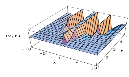
FIG. 2.: F(x,t) for the two bubbles with instanton-like form

FIG. 3.: F(x,t) at t=1.1 for the two bubbles with instanton-like form

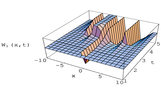
FIG. 4.: $W_{1}(x,t)=(2/g)xF(x,t)$ for the two bubbles with instanton-like form

The solution to Eq.(40) is given in Fig. 2. Note the development of a gluonic wall at the x=0 collision region. The development of the gluonic wall is clearly shown in Fig. 3, where F(x,t) at time t=1.1 is shown. In comparison to F(x,0), shown in Fig. 1 one can see how the instanton-like bubbles have collided and an interior gluonic wall produced. The wall is growing rapidly at this time, and due to the singularities in the solution the accuracy of the calculations for t $>$ 1.0 is limited, which is the origin of the violation of symmetry about x=0 in Fig. 3

The results for the function $W_{1}(x,t)=(2/g)xF(x,t)$, which is closely related to the color gluon field, are shown in Fig. 4. Note that the gluonic wall resembles a wall composed of instantons, as assumed in Ref. [13].

The gluonic Lagrangian density, ${\cal L}^{glue}$, for this solution is shown in Fig. 5, and the energy density, $T_{00}$, is shown in Fig. 6.

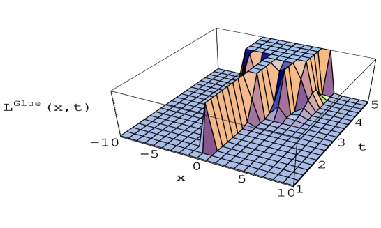
FIG. 5.: ${\cal L}^{glue}$(x,t), the gluonic Lagrangian density for the two bubbles with instanton-like form

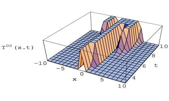
FIG. 6.: T₀₀(x,t), the energy density for the two bubbles with instanton-like form

In the light of the model calculations in Refs. [13],[5] these results are promising for studies of the CMBR correlations.

B Case II: Spontaneous symmetry breaking potential

In 1+1 dimension, the instanton-like ansatz of the previous subsection essentially takes the initial condition as $W_{1}(x,0)=xF(x,0)$ and $W_{0}(x,0)=0$ and observes the evolution of the instanton wall.

In this subsection, we discuss another scenario, which contrast to the instanton-like form but rather close to the Coleman-like model of scalar $\phi^{4}$ field theory [8]. As we shall show below, the SU(2) color gauge field given by Eq. (43) can be made to show the similar property of the scalar $\phi^{4}$ theory with the two degenerate vacua of the potential by taking $W_{1}(x,0)=w(x)$ and $W_{0}(x,0)=c$, where $c$ is a constant but not zero. We should note that the above initial condition satisfies the gauge condition, $\partial_{x}W_{0}(x,t)=\partial_{t}W_{1}(x,t)$ at $t=0$.

Then, the EOM given by Eq. (34) becomes

$$\partial_{x}w(x) = g(w^{2}-c^{2}),$$ (53)

$$\partial^{2}_{x}w(x) = 2g^{2}w(w^{2}-c^{2}),$$ (54)

at $t=0$. Note that the two coupled equations in Eq. (53) give the same initial condition for the field $w(x)$, which is obtained as

$$w(x) = -c\;{\rm tanh}[cg(x-x_{0})],$$ (55)

where $x_{0}$ is an integration constant. For this field configuration, the potential at $t=0$ can be easily obtained as

$$U(w)=\frac{g^{2}}{2}(w^{2}-c^{2})^{2}$$ (56)

up an additive constant.

We should note that the negative sign in Eq. (55) is uniquely determined from the 1st part of Eq. (53). This is very different from the usual scalar $\phi^{4}$ theory model where only the 2nd part of Eq. (53) represents the EOM of the theory and thus both signs could be solutions, i.e $w(x)=\pm c\tanh[cg(x-x_{0})]$. Our solution is not symmetric in x.

Figure  7 shows the potential as a function of $w$ for the particular values of $c=4,g=1$ and $x_{0}=3$. The potential has local minima at $w=\pm 4$, which correspond to the degenerate vacuum states.

Equation (55) is plotted in Fig. 8. This represents a field configuration consisting of two regions of space (bubbles) separated by a domain wall at $x=3$. We take this as the initial condition describing a collision of a bubble in vacuum state $w=4$ on the left of the domain wall with a bubble in vacuum state $w=-4$ on the right. Note that the two bubble walls collide at x=3,t=0, and that in our 1+1 model the bubbles have infinite radius. Thus our picture is a variation of the model of Ref[8].

FIG. 7.: Potential energy $U(w)$ with the doubly degenerate minima, $w=\pm 4$ at $t=0$.

FIG. 8.: Initial($t=0$) bubble configuration with the bubble wall at $x=3$ where the collision occurs.

Even though Eq. (53) does not allow solutions symmetric about $x=0$, rather than Eq.(55) we use a symmetric ansatz for $w(x)$:

$$w(x) = -c[1/2+{\rm tanh}[cg(x-x_{0})]]-c[1/2-{\rm tanh}[cg(x+x_{0})]]$$ (57)

to impose symmetric boundary condition, $W_{1}(-10,t)=W_{1}(10,t)$, as well as $\partial W_{i}(x,t=0)/\partial t=0(i=0,1)$. Otherwise, a non-symmetric boundary condition, such as $W_{1}(0,t)=-W(10,t)$ for the initial condition of Eq. (55), does not give a solution to the EOM given by Eq. (34). In the figures below we display only the solution for $x>0$, i.e. the solution with the correct initial $w(x)$ given by Eq. (55).

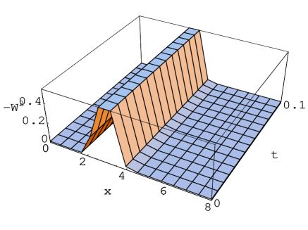
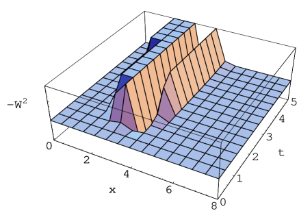
FIG. 9.: Evolution of the gluon field squared, $-W^{2}(x,t)=W^{2}_{0}(x,t)-W^{2}_{1}(x,t)$, with the domain wall-like form.

The evolution of the gluon field squared, $-W^{2}(x,t)=W^{2}_{0}-W^{2}_{1}$, given by the solution to Eq.( 34) with initial conditions given by Eq.( 57) in Minkowski space, is shown in Fig. 9 for two different time intervals, $0<t<0.1$(left) and $0<t<5$(right). Although this domain-wall like ansatz is quite different from the instanton ansatz, they show similar qualitative behavior of the field evolution.

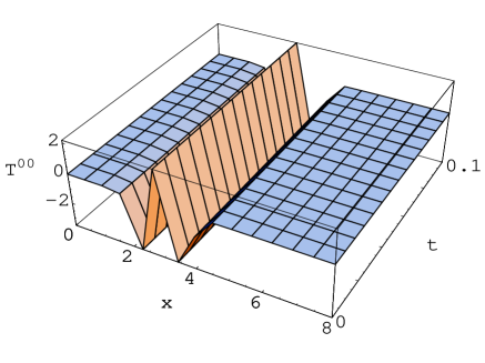
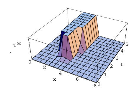
FIG. 10.: $T_{00}(x,t)$, the energy density with the domain wall-like form.

The energy density, $T_{00}(x,t)$ is shown in Fig. 10 for two different time intervals, $0<t<0.1$(left) and $0<t<5$(right). Again the energy density shown in Fig. 10 shows similar behavior to that in Fig.6 of instanton ansatz. We also note that the gluonic Lagrangian density, ${\cal L}^{glue}$, is very similar to the energy density profile as in the case of instanton-like form.

V Discussion and Conclusions

We have derived the equations of motion for a SU(2) color field theory, motivated and guided by the instanton model of QCD. Solutions in one space and one time dimension are studied as a simple picture for two QCD bubbles, with an initial structure resembling that of an instanton wall for each bubble, such as that assumed in Ref[13]. We indeed do find a gluonic structure evolving at the collision region, similar to that found in the effective field calculations of Ref[4]. In future research we shall investigate the nucleation of the bubbles and the possible creation of magnetic walls after the QCD phase transition for predictions of CMBR correlations.

This work was supported in part by the NSF grant PHY-00070888, in part by the DOE contract W-7405-ENG-36, and in part by the CosPA Project, Taiwan Minestry of education 89-N-FA01-1-3. LSK and MBJ acknowledge partial support by the LANL Institute for Nuclear and Particle Astrophysics and Cosmology, and HMC was supported in part by the Kyungpook National University Research Fund, 2003.

REFERENCES

• [1] S. Ijiri, Nucl. Phys B (Proc. Suppl.) 94, 19 (2001).
• [2] Y. Iwasaki $et.al$, Z. Phys. C 71, 343 (1996); C. DeTar, Nucl. Phys B (Proc. Suppl.) 42, 73 (1995), T. Blum $et.al.$, Phys. Rev. D 51, 5153 (1995).
• [3] G. Neergaard and Jes Madsen, Phys. Rev. D 62, 034005 (2000).
• [4] M.M. Forbes and A.R. Zhitnitsky, JHEP 0110, 013 (2001); Phys. Rev. Lett. 85, 5268 (2000); hep-ph/0102158 (2001).
• [5] L.S. Kisslinger, hep-ph/0212206 (2002).
• [6] J. Ignatius, K. Kajantie, H. Kurki-Suonio and M. Laine, Phys. Rev. D 50, 3738 (1994); J. C. Miller and L. Rezzolla, Phys. Rev. D 51, 4017 (1995); M.B. Christiansen abd J. Madsen, Phys. Rev. D 53, 5446 (1996).
• [7] S.W. Hawking, I.G. Moss and J.M. Stewart, Phys. Rev. D 26, 2681 (1977).
• [8] S. Colman, Phys. Rev. D 15, 2929 (1977); 16,1248(E); C. Callan, S. Coleman, Phys. Rev. D 16, 1762 (1977); “Aspects of Symmetry” (Cambridge University Press) (1985), Cpt. 7.
• [9] T.W.B. Kibble and A. Vilenkin, Phys. Rev. D 52, 679 (1995).
• [10] J. Ahonen and K. Enqvist, Phys. Rev. D 57, 664 (1998).
• [11] E.J. Copeland, P.M. Saffin and 0.Tornkvist, Phys. Rev. D 61, 105005 (2000).
• [12] E .Shuryak and I. Zahed, Phys. Rev. D 62, 085014 (2000), M.A. Nowak, E.V. Shuryak and I. Zahed , Phys. Rev. D 64, 034008 (2001).
• [13] L. S. Kisslinger, hep-ph/0202159 (2002).
• [14] A.A. Belavin, A.M. Polyakov, A.S. Schwartz and Yu.S. Tyupkin, Phys. Lett. B 59, 85 (1975).
• [15] G. ’t Hooft, Phys. Rev. D 14, 3432 (1976).
• [16] T. Schäfer and E. V. Shuryak, Rev. Mod. Phys. 70, 323 (1998).
• [17] M-C. Chu and S. Schramm, Phys. Rev. D 51, 4580 (1995); D 62, 094508 (2000); T. Schäfer and E.V. Shuryak, Phys. Rev. D 53, 6522 (1996).
• [18] A. D. Linde, Nucl. Phys. B 421, 421 (1983).