Technicolor corrections on $B_{s,d}\to\gamma\gamma$ decays in QCD factorization

Abstract

Within the framework of the Top-color-assisted Technicolor (TC2) model, we calculate the new physics contributions to the branching ratios ${\cal B}(B_{s,d}\to\gamma\gamma)$ and CP violating asymmetries $r^{-}_{CP}(B_{s,d}\to\gamma\gamma)$ in the QCD factorization based on the heavy-quark limit $m_{b}\gg\Lambda_{QCD}$. Using the considered parameter space, we find that (a) for both $B_{s}\to\gamma\gamma$ and $B_{d}\to\gamma\gamma$ decays, the new physics contribution can provide a factor of two to six enhancement to their branching ratios, (b) for the $B_{s}\to\gamma\gamma$ decay, its direct CP violation is very small in both the SM and TC2 model, and (c) the CP violating asymmetry $r^{-}_{CP}(B_{d}\to\gamma\gamma)$ is around the ten percent level in both the SM and TC2 model, but the sign of CP asymmetry in the TC2 model is different from that in the SM.

I Introduction

As is well known, the rare radiative decays of B mesons induced by the quark decay $b\to q\gamma$ ($q=d,s$) are very sensitive to the flavor structure of the standard model (SM) and to new physics beyond the SM. Both inclusive and exclusive processes, such as the decays $B\to X_{s}\gamma$, $X_{s}\gamma\gamma$ and $B_{s,d}\to\gamma\gamma$, have been studied in great detail [1, 2, 3, 4, 5, 6, 7, 8, 9, 10, 11].

The inclusive decay $B\to X_{s}\gamma$ is measured experimentally with increasing accuracy[12]. The world average as given by the 2002 Particle Data Group ( PDG2002 ) [13] is

$${\cal B}(B\to X_{s}\gamma)=(3.3\pm 0.40)\times 10^{-4},$$ (1)

which is quite consistent with the next-to-leading order (NLO) standard model prediction [4]

$${\cal B}(B\to X_{s}\gamma)^{TH}=(3.29\pm 0.34)\times 10^{-4},$$ (2)

Obviously, there is only small room left for new physics effects in flavor-changing neutral current processes based on the $b\to s$ transition. In other words, the excellent agreement between SM theory and experimental data results in a strong constraint on many new physics models beyond the SM.

Within the SM, the electroweak contributions to $b\to s\gamma\gamma$ and $B\to\gamma\gamma$ decays have been calculated some time ago[1]; the leading-order QCD corrections and the long-distance contributions were evaluated recently by several groups[6, 14]. The new physics corrections were also considered, for example, in the two-Higgs doublet model [15, 16] and the supersymmetric model [17].

On the experimental side, only upper limits ($90\%C.L.$) on the branching ratios of $B_{s,d}\to\gamma\gamma$ are currently available

$${\cal B}(B_{s}\to\gamma\gamma) < 1.48\times 10^{-4},\cite[cite]{[\@@bibref{Number}{cleo95}{}{}]}$$ (3)

$${\cal B}(B_{d}\to\gamma\gamma) < 1.7\times 10^{-6},\cite[cite]{[\@@bibref{Number}{babar01}{}{}]}$$ (4)

which are roughly two orders above the SM predictions [1, 6, 8, 9]. These radiative decays are indeed very interesting because (a) these decays have a very clean signal where two monochromatic energetic photons are produced precisely back-to-back in the rest frame of B meson; (b) these exclusive decays also allow us to study the CP violating effects as the two photon system can be in a CP-even or CP-odd state; (c) since $B_{s}\to\gamma\gamma$ depends on the same set of Wilson coefficients as $B\to X_{s}\gamma$, its sensitivity to new physics beyond the SM complements the corresponding sensitivity in $B\to X_{s}\gamma$; and (d) the smallness of the branching ratios can be compensated by the very high statistics expected at the current B factory experiments and future hadron colliders.

In this paper, we present our calculation of branching ratios and CP-violating asymmetries for rare exclusive decays $B_{s,d}\to\gamma\gamma$ in the framework of the Top-color-assisted Technicolor (TC2) model [20] by employing the QCD factorization based on the heavy-quark limit $m_{b}\gg\Lambda_{QCD}$ [8, 9].

This paper is organized as follows: In Sec. II, we give a brief review about the SM predictions for the branching ratios and CP asymmetries of $B_{s,d}\to\gamma\gamma$ decays. In Sec. III, we present the basic ingredients of the TC2 model, and evaluate the new penguin diagrams. After studying the constraint on the TC2 model by considering the data of $B_{d}^{0}-\bar{B}^{0}_{d}$ mixing and $B\to X_{s}\gamma$ decay, we find the Wilson coefficients $C_{7}$ and $C_{8}$ with the inclusion of the new physics (NP) contribution. In Sec. 4, we show the numerical results of branching ratios and CP-violating asymmetries for $B_{s,d}\to\gamma\gamma$ decays. The discussions and conclusions are included in the final section.

II $B_{s,d}\to\gamma\gamma$ decays in the SM

In this section, based on currently available studies, we present the formulae for exclusive decay $B_{s,d}\to\gamma\gamma$ in the framework of SM.

A Effective Hamiltonian for inclusive $b\to s\gamma\gamma$ decay

We know that the quark level processes $b\to s\gamma,s\gamma\gamma$ and the exclusive decays $B_{s,d}\to\gamma\gamma$ have a close relation. Up to the order $1/m^{2}_{W}$, the effective Hamiltonian for the decay $b\to s\gamma\gamma$ is identical to the one for $B\to X_{s}\gamma$ transition [1, 7]

$${\cal H}_{eff}(b\to s\gamma)={\cal H}_{eff}(b\to s\gamma\gamma)+{\cal O}\left(\frac{1}{m_{W}^{2}}\right).$$ (5)

This can be understood by either applying the equation of motion [21] or by applying an extension of Low’s low energy theorem[22].

Up to corrections of order $1/m_{W}^{2}$, the effective Hamiltonian for $b\to s\gamma\gamma$ is just the one for $b\to s\gamma$ and takes the form

$${\cal H}_{eff}=\frac{G_{F}}{\sqrt{2}}\sum_{p=u,c}\lambda_{p}^{(s)}\left[C_{1}(\mu)Q^{p}_{1}+C_{2}(\mu)Q^{p}_{2}+\sum_{i=3,\ldots,8}C_{i}(\mu)Q_{i}\right],$$ (6)

where $\lambda_{p}^{(s)}=V^{*}_{ps}V_{pb}$ is the Cabibbo-Kobayashi-Maskawa (CKM) factor. And the current-current, QCD penguin, electromagnetic and chromomagnetic dipole operators are given by

$$Q^{p}_{1} = (\bar{s}_{\alpha}p_{\beta})_{V-A}(\bar{p}_{\beta}b_{\alpha})_{V-A},$$ (7)

$$Q^{p}_{2} = (\bar{s}p)_{V-A}(\bar{p}b)_{V-A},$$ (8)

$$Q_{3} = (\bar{s}b)_{V-A}\sum_{q=u,d,s,c,b}(\bar{q}q)_{V-A},$$ (9)

$$Q_{4} = (\bar{s}_{\alpha}b_{\beta})_{V-A}\sum_{q=u,d,s,c,b}(\bar{q}_{\beta}q_{\alpha})_{V-A},$$ (10)

$$Q_{5} = (\bar{s}b)_{V-A}\sum_{q=u,d,s,c,b}(\bar{q}q)_{V+A},$$ (11)

$$Q_{6} = (\bar{s}_{\alpha}b_{\beta})_{V-A}\sum_{q=u,d,s,c,b}(\bar{q}_{\beta}q_{\alpha})_{V+A},$$ (12)

$$Q_{7} = \frac{e}{4\pi^{2}}\,\bar{s}_{\alpha}\sigma^{\mu\nu}\left(m_{b}R+m_{s}L\right)b_{\alpha}\,F_{\mu\nu}\,,$$ (13)

$$Q_{8} = \frac{g_{s}}{4\pi^{2}}\,\bar{s}_{\alpha}\sigma^{\mu\nu}\left(m_{b}R+m_{s}L\right)T^{a}_{\alpha\beta}b_{\beta}\,G^{a}_{\mu\nu}\,,$$ (14)

where $\alpha$ and $\beta$ are color indices, $\alpha=1,\ldots,8$ labels $SU(3)_{c}$ generators, $e$ and $g_{s}$ refer to the electromagnetic and strong coupling constants, and $L,R=(1\mp\gamma_{5})/2$, while $F_{\mu\nu}$ and $G^{a}_{\mu\nu}$ denote the photonic and gluonic field strength tensors, respectively. In $Q_{7,8}$, the terms proportional to $m_{s}$ are usually neglected because of the strong suppression $m_{s}^{2}/m_{b}^{2}$. The effective Hamiltonian for $b\to d\gamma\gamma$ is obtained from Eqs.(6) - (14) by the replacement $s\to d$.

The Wilson coefficients $C_{i}(\mu)$ in Eq.(6) are known currently at next-to-leading order (NLO) [2, 3]. Within the SM and at scale $m_{W}$, the Wilson coefficients $C_{i}(m_{W})$ at the leading order (LO) approximation have been given for example in [3],

$$C_{i}(m_{W}) = 0\ \ \ (i=1,3,4,5,6),$$ (15)

$$C_{2}(m_{W}) = 1,,$$ (16)

$$C_{7}(m_{W}) = \frac{-7x_{t}+5x_{t}^{2}+8x_{t}^{3}}{24(1-x_{t})^{3}}-\frac{2x_{t}^{2}-3x_{t}^{3}}{4(1-x_{t})^{4}}\log[x_{t}],$$ (17)

$$C_{8}(m_{W}) = \frac{-2x_{t}-5x_{t}^{2}+x_{t}^{3}}{8(1-x_{t})^{3}}-\frac{3x_{t}^{2}}{4(1-x_{t})^{4}}\log[x_{t}],$$ (18)

where $x_{t}=m_{t}^{2}/m_{W}^{2}$.

By using QCD renormalization group equations[3], it is straightforward to run Wilson coefficients $C_{i}(m_{W})$ from the scale $\mu={\cal O}(m_{W})$ down to the lower scale $\mu={\cal O}(m_{b})$. The leading order results for the Wilson coefficients $C_{i}(\mu)$ with $\mu\approx m_{b}$ are of the form [3]

$$C_{j}(\mu) = \sum_{i=1}^{8}k_{ji}\eta^{a_{i}}\ \ \ (j=1,\ldots,6),$$ (19)

$$C_{7}(\mu) = \eta^{16/23}C_{7}(m_{W})+\frac{8}{3}\left(\eta^{14/23}-\eta^{16/23}\right)C_{8}(m_{W})+\sum_{i=1}^{8}h_{i}\eta^{a_{i}}\,,$$ (20)

$$C_{8}(\mu) = \eta^{14/23}C_{8}(m_{W})+\sum_{i=1}^{8}\bar{h}_{i}\eta^{a_{i}}\,,$$ (21)

where $\eta=\alpha_{s}(m_{W})/\alpha_{s}(\mu)$, and the magic numbers are [3]

$$a_{i} = (14/23,16/23,6/23,-12/23,0.4086,-0.4230,-0.8994,0.1456)\,,$$ (22)

$$h_{i} = (2.2996,-1.0880,-3/7,-1/14,-0.6494,-0.0380,-0.0185,-0.0057)\,,$$ (23)

$$\bar{h}_{i} = (0.8623,0,0,0,-0.9135,0.0873,-0.0571,0.0209)\,,$$ (24)

$$k_{ji} = \left(\begin{array}[]{cccc cccc}0&0&1/2&-1/2&0&0&0&0\\ 0&0&1/2&1/2&0&0&0&0\\ 0&0&-1/14&1/6&0.0510&-0.1403&-0.0113&0.0054\\ 0&0&-1/14&-1/6&0.0984&0.1214&0.0156&0.0026\\ 0&0&0&0&-0.0397&0.0117&-0.0025&0.0304\\ 0&0&0&0&0.0335&0.0239&-0.0462&-0.0112\\ \end{array}\right)\quad.$$ (31)

The numerical results of the LO Wilson coefficients $C_{i}(\mu)$ obtained by using the input parameters as given in Table I are listed in Table II for $\mu=m_{b}/2,m_{b}$ and $2m_{b}$, respectively.

B $B_{s,d}\to\gamma\gamma$ decays in the SM

Based on the effective Hamiltonian for the quark level process $b\to s(d)\gamma\gamma$, one can write down the amplitude for $B_{s,d}\to\gamma\gamma$ and calculate the branching ratios and CP violating asymmetries once a method is derived for computing the hadronic matrix elements. There exist so far two major approaches for the theoretical treatments of exclusive decay $B\to\gamma\gamma$.

The first approach was proposed ten years ago and has been employed by many authors [1, 6]. Under this approach, one simply evaluates the hadronic element of the amplitudes for one-particle reducible (1PR) and one-particle irreducible (1PI) diagrams, relying on a phenomenological model. One can work, for example, in the weak binding approximation and assume that both the $b$ and the light $q$ quarks are at rest in the $B_{q}$ meson[23]. From the heavy quark effective theory(HQET), for instance, one can also assume that the velocity of the $b$ quark coincides with the velocity of the $B_{q}$ meson up to a residual momentum of $\Lambda_{QCD}$. Both pictures are compatible up to corrections of order ($\Lambda_{QCD}/m_{b}$) [23]. One typical numerical result obtained by employing this approach is

$${\cal B}(B_{s}\to\gamma\gamma)\approx(2-8)\times 10^{-7}$$ (32)

after inclusion of LO QCD corrections [23]. There are also many works concerning the estimation of the long distance contributions to $B\to\gamma\gamma$ decay[14].

In the first approach, one has to employ hadronic models to describe the $B_{q}$ ($q=s,d$) meson bound state dynamics. It is thus impossible for one to separate clearly the short- and long-distance dynamics and to make distinctions between the model-dependent and model-independent features.

The second approach was proposed recently by Bosch and Buchalla[8, 9]. They analyzed the $B_{s,d}\to\gamma\gamma$ decays in QCD factorization approach based on the heavy quark limit $m_{b}\gg\Lambda_{QCD}$. Under this approach, one can systematically separate perturbatively calculable hard scattering kernels from the nonperturbative B-meson wave function. Power counting in $\Lambda_{QCD}/m_{b}$ allows one to identify leading and subleading contributions to $B\to\gamma\gamma$. In this paper, we will employ the Bosch and Buchalla (BB) approach to calculate the Technicolor corrections to $B_{s,d}\to\gamma\gamma$ decays.

From Refs.[8, 9], one knows that (a) only one 1PR diagram [ Fig. 1(a) ] contributes at leading power; (b) the most important subleading contributions induced by the 1PR [Fig. 1(b) ] and 1PI diagrams [Fig. 1(c) ] can also be calculated; and (c) the direct CP violation of $B_{d}\to\gamma\gamma$ can reach the $10\%$ level.

The amplitude for the $B\to\gamma\gamma$ decay has the general structure[8]

$${\cal A}(\bar{B}\to\gamma(k_{1},\epsilon_{1})\gamma(k_{2},\epsilon_{2}))=\frac{G_{F}}{\sqrt{2}}\frac{\alpha_{em}}{3\pi}f_{B}\frac{1}{2}\langle\gamma\gamma|A_{+}F_{\mu\nu}F^{\mu\nu}-i\,A_{-}F_{\mu\nu}\tilde{F}^{\mu\nu}|0\rangle.$$ (33)

Here $F^{\mu\nu}$ and $\tilde{F}^{\mu\nu}=\varepsilon^{\mu\nu\lambda\rho}F_{\lambda\rho}/2$ are the photon field strength tensor and its dual with $\varepsilon^{0123}=-1$. The branching ratio of $B_{q}\to\gamma\gamma$ decay with $q=s,d$ is then given by

$${{\cal B}}(\bar{B}_{q}\to\gamma\gamma)=\tau_{B_{q}}\,\frac{G^{2}_{F}m^{3}_{B_{q}}f^{2}_{B_{q}}\alpha_{em}^{2}}{288\pi^{3}}\left(|A_{+}|^{2}+|A_{-}|^{2}\right)$$ (34)

where $G_{F}$ is the Fermi constant, $\alpha_{em}$ is the fine structure constant, $\tau_{B_{q}}$ is the lifetime of $B_{q}$ meson, and $m_{B_{q}}$ and $f_{B_{q}}$ are the mass and decay constant of the $B_{q}$ meson, respectively. The values of all input parameters are listed in Table I.

The matrix elements of the operators $Q_{i}$ in Eq.(6) can be written as

$$\langle\gamma(\epsilon_{1})\gamma(\epsilon_{2})|Q_{i}|\bar{B}\rangle=f_{B}\int^{1}_{0}d\xi\,T^{\mu\nu}_{i}(\xi)\,\Phi_{B}(\xi)\epsilon_{1\mu}\epsilon_{2\nu}$$ (35)

where the $\epsilon_{i}$ are the polarization 4-vectors of the photons, $\Phi_{B}\equiv\Phi_{B1}$ is the leading twist light-cone distribution amplitude of the $B$ meson, and $T^{\mu\nu}_{i}(\xi)$ is the hard-scattering kernel describing the hard-spectator contribution.

By explicit calculations as were done in Ref.[8], the quantities $A_{\pm}$ in Eq.(34) are of the form

$$A_{+} = \lambda_{u}^{(q)}A_{+}^{u}+\lambda_{c}^{(q)}A_{+}^{c},$$ (36)

$$A_{-} = \lambda_{u}^{(q)}A_{-}^{u}+\lambda_{c}^{(q)}A_{-}^{c},$$ (37)

with

$$A^{p}_{+} = -C_{7}\frac{m_{B}}{\lambda_{B}}+\left(C_{5}+3C_{6}\right)\left[\frac{1}{2}g(1)-\frac{1}{3}\right],$$ (38)

$$A^{p}_{-} = -C_{7}\frac{m_{B}}{\lambda_{B}}-\frac{2}{3}\left(C_{2}+3C_{1}\right)g(z_{p})-\left(C_{3}-C_{5}\right)\left[2g(z_{c})+\frac{5}{6}g(1)\right]$$ (40)

$$-\left(C_{4}-C_{6}\right)\left[\frac{2}{3}g(z_{c})+\frac{7}{6}g(1)\right]+\frac{20}{3}C_{3}+4C_{4}-\frac{16}{3}C_{5},$$

where $z_{p}=m_{p}^{2}/m_{b}^{2}$ for $p=u,c$, and

$$g(z)=-2+4z\left[Li_{2}\left(\frac{2}{1-\sqrt{1-4z+i\epsilon}}\right)+Li_{2}\left(\frac{2}{1+\sqrt{1-4z+i\epsilon}}\right)\right]$$ (41)

and $Li_{2}(x)$ is the dilogarithm function. It is easy to see that $A^{u}_{+}=A^{c}_{+}$, but $A^{u}_{-}\neq A^{c}_{-}$. The function $g(z)$ has an imaginary part for $0<z<1/4$, while $g(0)=-2$ and $g(1)=2(\pi^{2}-9)/9$.

The first term of $A_{\pm}^{p}$ is the leading power contribution from the 1PR diagram [ Fig.1(a) ] of the penguin operator $Q_{7}$, the remaining terms of $A_{\pm}^{p}$ represent the subleading contributions from the 1PR diagram [ Fig.1(b) ] with the operator $Q_{7}$ where the second photon is emitted from the $b$ quark line, and from the 1PI diagram [ Fig.1(c) ] induced by insertion of four-quark operators $Q_{i}$. From the formulas as given in Eq.(34) and Eqs.(36) - (40), we find the numerical results of the branching ratios in SM

$${{\cal B}}(\bar{B}_{s}\to\gamma\gamma) = \left[1.2^{+2.4}_{-0.6}(\Delta\lambda_{B})^{+0.3}_{-0.2}(\Delta\mu)\pm 0.3(\Delta f_{B_{s}})\pm 0.02(\Delta\gamma)\right]\times 10^{-6},$$ (42)

$${{\cal B}}(\bar{B}_{d}\to\gamma\gamma) = \left[3.2^{+6.6}_{-1.6}(\Delta\lambda_{B})^{+0.8}_{-0.6}(\Delta\mu)^{+1.0}_{-0.9}(\Delta f_{B_{d}})^{+1.1}_{-0.8}(\Delta\gamma)\right]\times 10^{-8},$$ (43)

where the central values of branching ratios are obtained by using the central values of input parameters as given in Table I, and the errors correspond to $\Delta\lambda_{B}=\pm 0.15$ GeV, $m_{b}/2\leq\mu\leq 2m_{b}$, $\Delta f_{B_{d}}=\Delta f_{B_{s}}=\pm 0.03$ GeV, respectively. For the CKM angle $\gamma$, we consider the range of $\gamma=(60\pm 20)^{\circ}$ according to the global fit result [13]. Obviously, the dominant errors are induced by the uncertainty of hadronic parameter $\lambda_{B}$, the renormalization scale $\mu$ and decay constant $f_{B_{q}}$. The error induced by $\Delta\gamma$ is about $30\%$ for $B_{d}$ decay, but very small for $B_{s}$ decay. The errors due to the uncertainty of other input parameters are indeed very small and can be neglected.

Now we consider the CP violating asymmetries of $B_{s,d}\to\gamma\gamma$ decays. Following the definitions of Ref.[8], the subscripts $\pm$ on $A_{\pm}$ for $\bar{B}\to\gamma\gamma$ decay denote the CP properties of the corresponding two-photon final states, while $\bar{A}_{\pm}$ refer to the CP conjugated amplitudes for the decay $B\to\gamma\gamma$ (decaying $\bar{b}$ antiquark). Then the deviation of the ratios

$$r^{\pm}_{CP}=\frac{|A_{\pm}|^{2}-|\bar{A}_{\pm}|^{2}}{|A_{\pm}|^{2}+|\bar{A}_{\pm}|^{2}}$$ (44)

from zero is a measure of direct CP violation. Since $A_{+}^{p}=\bar{A}_{+}^{p}$, $r^{+}_{CP}$ is always zero. For $r^{-}_{CP}$ of $B_{d}\to\gamma\gamma$ decay, however, it can be rather large. By using the central values of input parameters as given in Table I and assuming $\gamma=60^{\circ}$, we find

$$r^{-}_{CP}(B_{s}\to\gamma\gamma) = \left[0.39^{+0.25}_{-0.28}(\Delta\mu)^{+0.16}_{-0.11}(\Delta\lambda_{B})^{+0.06}_{-0.11}(\Delta\gamma)\right]\%,$$ (45)

$$r^{-}_{CP}(B_{d}\to\gamma\gamma) = \left[-10.2^{+7.3}_{-6.6}(\Delta\mu)^{+4.3}_{-4.0}(\Delta\lambda_{B})^{+1.4}_{-0.1}(\Delta\gamma)\right]\%$$ (46)

It is easy to see that the direct CP violating asymmetry for $B_{s}\to\gamma\gamma$ decay is small, $\sim 1\%$, and cannot be detected by experiments. For $B_{d}\to\gamma\gamma$ decay. however, its CP violation can be rather large, around $-10\%$ for $\gamma\sim 60^{\circ}$. But the much smaller branching ratio is a great challenge for the current and future experiments.

In Fig. 2, we show the CKM angle $\gamma-$ and $\mu$-dependence of $r^{-}_{CP}(B_{d}\to\gamma\gamma)$. The dotted, short-dashed and solid curves show the SM predictions of $r^{-}_{CP}(B_{d}\to\gamma\gamma)$ for $\mu=m_{b}/2,m_{b}$ and $2m_{b}$, respectively. The CP violating asymmetry even can reach $-17\%$ for CKM angle $\gamma\approx 50^{\circ}$, the value preferred by the global fit [24] and by the analysis based on the measurements of branching ratios of $B\to K\pi$ decays [25]. The value of $r^{-}_{CP}(B_{d}\to\gamma\gamma)$ here is the same as that given in Ref.[8] for $\mu=m_{b}$, but opposite with what was given in Ref.[8] for $\mu=m_{b}/2$ and $2m_{b}$, respectively.

III $B_{s,d}\to\gamma\gamma$ decays in TC2 model

In this section, we calculate the loop corrections to $B_{s,d}\to\gamma\gamma$ decays in TC2 model.

A TC2 model

Apart from some differences in group structure and/or particle contents, all TC2 models [20, 26] have the following common features: (a) strong Top-color interactions, broken near 1 TeV, induce a large top condensate and all but a few GeV of the top quark mass, but contribute little to electroweak symmetry breaking; (b) technicolor [27] interactions are responsible for electroweak symmetry breaking, and extended technicolor (ETC) [28] interactions generate the masses of all quarks and leptons, except that of the top quarks; (c) there exist top pions $\tilde{\pi}^{\pm}$ and $\tilde{\pi}^{0}$ with a decay constant $F_{Q}\approx(40-50)$ GeV. In this paper we will chose the well-motivated and most frequently studied TC2 model proposed by Hill [20] to calculate the contributions to the rare exclusive B decays from the relatively light charged pseudo-scalars. It is straightforward to extend the studies in this paper to other TC2 models.

In the TC2 model[20], after integrating out the heavy coloron and $Z^{\prime}$, the effective four-fermion interactions have the form [29]

$${\cal L}_{eff}=\frac{4\pi}{M_{V}^{2}}\left\{\left(\kappa+\frac{2\kappa_{1}}{27}\right)\overline{\psi}_{L}t_{R}\overline{t}_{R}\psi_{L}+\left(\kappa-\frac{\kappa_{1}}{27}\right)\overline{\psi}_{L}b_{R}\overline{b}_{R}\psi_{L}\right\},$$ (47)

where $\kappa=(g_{3}^{2}/4\pi)\cot^{2}\theta$ and $\kappa_{1}=(g_{1}^{2}/4\pi)\cot^{2}\theta^{\prime}$, and $M_{V}$ is the mass of coloron $V^{\alpha}$ and $Z^{\prime}$. The effective interactions of Eq. (47) can be written in terms of two auxiliary scalar doublets $\phi_{1}$ and $\phi_{2}$. Their couplings to quarks are given by [30]

$${\cal L}_{eff}=\lambda_{1}\overline{\psi}_{L}\phi_{1}\overline{t}_{R}+\lambda_{2}\overline{\psi}_{L}\phi_{2}\overline{b}_{R},$$ (48)

where $\lambda_{1}^{2}=4\pi(\kappa+2\kappa_{1}/27)$ and $\lambda_{2}^{2}=4\pi(\kappa-\kappa_{1}/27)$. At energies below the top-color scale $\Lambda\sim 1$ TeV the auxiliary fields acquire kinetic terms, becoming physical degrees of freedom. The properly renormalized $\phi_{1}$ and $\phi_{2}$ doublets take the form

$$\phi_{1}=\left(\begin{array}[]{cc}F_{Q}+\frac{1}{\sqrt{2}}(h_{t}+i\tilde{\pi}^{0})\\ \tilde{\pi}^{-}\end{array}\right),\ \ \phi_{2}=\left(\begin{array}[]{cc}\tilde{H}^{+}\\ \frac{1}{\sqrt{2}}(\tilde{H}^{0}+i\tilde{A}^{0})\end{array}\right),$$ (53)

where $\tilde{\pi}^{\pm}$ and $\tilde{\pi}^{0}$ are the top pions, $\tilde{H}^{\pm,0}$ and $\tilde{A}^{0}$ are the b pions, $h_{t}$ is the top Higgs boson, and $F_{Q}\approx 50$ GeV is the top pion decay constant.

From Eq. (48), the couplings of top pions to t and b quark can be written as [20]

$$\frac{m_{t}^{*}}{F_{Q}}\left[i\;\bar{t}t\tilde{\pi}^{0}+i\;\overline{t}_{R}b_{L}\tilde{\pi}^{+}+i\;\frac{m_{b}^{*}}{m_{t}^{*}}\overline{t}_{L}b_{R}\tilde{\pi}^{+}+H.c.\right],$$ (54)

where $m_{t}^{*}=(1-\epsilon)m_{t}$ and $m_{b}^{*}\approx 1$ GeV denote the masses of top and bottom quarks generated by top-color interactions.

For the mass of top pions, the current $1-\sigma$ lower mass bound from the Tevatron data is $m_{\tilde{\pi}}\geq 150$ GeV [26], while the theoretical expectation is $m_{\tilde{\pi}}\approx(150-300GeV)$[20]. For the mass of b pions, the current theoretical estimation is $m_{\tilde{H}^{0}}\approx m_{\tilde{A}^{0}}\approx(100-350)GeV$ and $m_{\tilde{H}}=m_{\tilde{H}^{0}}^{2}+2m_{t}^{2}$ [30]. For the technipions $\pi_{1}^{\pm}$ and $\pi_{8}^{\pm}$, the theoretical estimations are $m_{\pi_{1}}\geq 50GeV$ and $m_{\pi_{8}}\approx 200GeV$[31, 32]. The effective Yukawa couplings of ordinary technipions $\pi_{1}^{\pm}$ and $\pi_{8}^{\pm}$ to fermion pairs, as well as the gauge couplings of unit-charged scalars to gauge bosons $\gamma,Z^{0}$ and $gluon$ are basically model-independent, can be found in Refs.[31, 32, 33].

At low energy, potentially large flavor-changing neutral currents (FCNC) arise when the quark fields are rotated from their weak eigenbasis to their mass eigenbasis, realized by the matrices $U_{L,R}$ for the up-type quarks, and by $D_{L,R}$ for the down-type quarks. When we make the replacements, for example,

$$b_{L}\to D_{L}^{bd}d_{L}+D_{L}^{bs}s_{L}+D_{L}^{bb}b_{L},$$ (55)

$$b_{R}\to D_{R}^{bd}d_{R}+D_{R}^{bs}s_{R}+D_{R}^{bb}b_{R},$$ (56)

the FCNC interactions will be induced. In TC2 model, the corresponding flavor changing effective Yukawa couplings are

$$\frac{m_{t}^{*}}{F_{Q}}\left[i\;\tilde{\pi}^{+}(D_{L}^{bs}\bar{t}_{R}s_{L}+D_{L}^{bd}\bar{t}_{R}d_{L})+i\;\tilde{H}^{+}(D_{R}^{bs}\bar{t}_{L}s_{R}+D_{R}^{bd}\bar{t}_{L}d_{R})+H.c.\right].$$ (57)

For the mixing matrices in the TC2 model, authors usually use the “square-root ansatz”: to take the square root of the standard model CKM matrix ($V_{CKM}=U_{L}^{+}D_{L}$) as an indication of the size of realistic mixings. It should be denoted that the square root ansatz must be modified because of the strong constraint from the data of $B^{0}-\overline{B^{0}}$ mixing [30, 34, 35]. In the TC2 model, the neutral scalars $\tilde{H}^{0}$ and $\tilde{A}^{0}$ can induce a contribution to the $B_{q}^{0}-\overline{B_{q}^{0}}$ ($q=d,s$) mass difference [29, 30]

$$\frac{\Delta M_{B_{q}}}{M_{B_{q}}}=\frac{7}{12}\frac{m_{t}^{2}}{F_{Q}^{2}m^{2}_{\tilde{H}^{0}}}\delta_{bq}B_{B_{q}}F_{B_{q}}^{2},$$ (58)

where $M_{B_{q}}$ is the mass of $B_{q}$ meson, $F_{B_{q}}$ is the $B_{q}$-meson decay constant, $B_{B_{q}}$ is the renormalization group invariant parameter, and $\delta_{bq}\approx|D_{L}^{bq}D_{R}^{bq}|$. For the $B_{d}$ meson, using the experimental measurement of $\Delta M_{B_{d}}=(3.22\pm 0.05)\times 10^{-10}MeV$[13] and setting $F_{Q}=45GeV$, $\sqrt{B_{B_{d}}}F_{B_{d}}=200MeV$, one has the bound $\delta_{bd}\leq 0.82\times 10^{-7}$ for $m_{\tilde{H}^{0}}\leq 600GeV$. This is an important and strong bound on the product of mixing elements $D_{L,R}^{bd}$. As pointed in [29], if one naively uses the square-root ansatz for both $D_{L}$ and $D_{R}$, this bound is violated by about 2 orders of magnitude. By taking into account above experimental constraint, we naturally set that $D_{R}^{ij}=0$ for $i\neq j$. Under this assumption, only the charged technipions $\pi_{1}^{\pm},\pi_{8}^{\pm}$ and the charged top pions $\tilde{\pi}^{\pm}$ contribute to the decays studied here through penguin diagrams.

B Constraint on TC2 model from $B\to X_{s}\gamma$ decay

The constraint on both $D_{L}$ and $D_{R}$ from the experimental data of $B\to X_{s}\gamma$ decay is much weaker than that from the $B^{0}-\bar{B}^{0}$ mixings[29]. On the other hand, one can draw strong constraint on the mass of top-pion $m_{\tilde{\pi}}$ from the well measured $B\to X_{s}\gamma$ decay by setting $D_{L}^{bd}=V_{td}/2$, $D_{L}^{bs}=V_{ts}/2$, $F_{Q}=45$ GeV and $\epsilon=0.05\pm 0.03$.

In this subsection, we firstly calculate the new physics contributions to the Wilson coefficients $C_{7}(m_{W})$ and $C_{8}(m_{W})$. And then we draw the constraint on the mass $m_{\tilde{\pi}}$ by comparing the theoretical prediction of ${{\cal B}}(B\to X_{s}\gamma)$ with the measured value as given in Eq.(1).

The new photonic- and gluonic-penguin diagrams can be obtained from the corresponding penguin diagrams in the SM by replacing the internal $W^{\pm}$ lines with the unit-charged scalar ($\pi_{1}^{\pm},\pi_{8}^{\pm}$ and $\tilde{\pi}^{\pm}$ ) lines, as shown in Fig. 3. For details of the analytical calculations, one can see Ref.[36].

By evaluating the new $\gamma$-penguin and $gluon$-penguin diagrams induced by the exchanges of three kinds of charged pseudoscalars ($\tilde{\pi}^{\pm},\pi_{1}^{\pm},\pi_{8}^{\pm}$), we find that

$$C_{7}(m_{W})^{TC2} = \frac{1}{8\sqrt{2}G_{F}F_{Q}^{2}}H(y_{t})+\frac{1}{6\sqrt{2}G_{F}F_{\pi}}\left[H(\eta_{t})+8H(\xi_{t})\right],$$ (59)

$$C_{8}(m_{W})^{TC2} = \frac{1}{8\sqrt{2}G_{F}F_{Q}^{2}}K(y_{t})+\frac{1}{6\sqrt{2}G_{F}F_{\pi}}\left[K(\eta_{t})+8K(\xi_{t})+9L(\xi_{t})\right],$$ (60)

where $y_{t}=m_{\tilde{\pi}}^{2}/((1-\epsilon)m_{t})^{2}$, $\eta_{t}=m_{\pi_{1}}^{2}/(\epsilon m_{t})^{2}$, $\xi_{t}=m_{\pi_{8}}^{2}/(\epsilon m_{t})^{2}$, while the functions $H(x)$, $K(x)$ and $L(x)$ are

$$H(x) = \frac{22-53x+25x^{2}}{36(1-x)^{3}}+\frac{3x-8x^{2}+4x^{3}}{6(1-x)^{4}}\log[x],$$ (61)

$$K(x) = \frac{5-19x+20x^{2}}{12(1-x)^{3}}-\frac{x^{2}-2x^{3}}{2(1-x)^{4}}\log[x],$$ (62)

$$L(x) = \frac{4-5x-5x^{2}}{12(1-x)^{3}}+\frac{x-2x^{2}}{2(1-x)^{4}}\log[x].$$ (63)

It is easy to show that the charged top-pion $\tilde{\pi}^{\pm}$ strongly dominate the new physics contributions to the Wilson coefficients $C_{7}(m_{W})$ and $C_{8}(m_{W})$, while the technipions play a minor rule only, less than $5\%$ of the total NP correction. We therefore fix the masses of $\pi_{1}^{\pm}$ and $\pi_{8}^{\pm}$ in the range of $m_{\pi_{1}}=200\pm 100$ GeV and $m_{\pi_{8}}=400\pm 100$ GeV, as listed in Table III. At the leading order, the charged-scalars do not contribute to the remaining Wilson coefficients $Q_{1}-Q_{6}$.

When the new physics contributions are taken into account, the Wilson coefficients $C_{7}(m_{W})$ and $C_{8}(m_{W})$ can be defined as the following,

$$C_{7}(m_{W})^{Tot} = C_{7}(m_{W})^{SM}+C_{7}(m_{W})^{TC2},$$ (64)

$$C_{8}(m_{W})^{Tot} = C_{8}(m_{W})^{SM}+C_{8}(m_{W})^{TC2},$$ (65)

where $C_{7,8}^{SM}$ have been given in Eqs.(17), (18). Explicit calculations show that the Wilson coefficients $C_{7,8}^{TC2}$ have the opposite sign with their SM counterparts, and therefore they will interfere destructively. The QCD running of $C_{7}^{tot}$ from the energy scale $m_{W}$ to $\mu\approx m_{b}$ is the same as the case of SM.

Using the NLO formulas as presented in Ref.[4] for the $B\to X_{s}\gamma$ decay, we find the numerical results for the branching ratios ${{\cal B}}(B\to X_{s}\gamma)$ in both the SM and the TC2 model, as illustrated in Fig. 4, where we use the central values of input parameters as given in Table I and Table III. The three curves correspond to $\mu=m_{b}/2$ (short-dashed curve), $\mu=m_{b}$ (solid curve) and $\mu=2m_{b}$ (dot-dashed curve), respectively. The band between two horizontal dotted-lines shows the SM prediction ${{\cal B}}(B\to X_{s}\gamma)=(3.29\pm 0.34)\times 10^{-4}$ [4], while the band between two horizontal solid lines shows the data, $2.5\times 10^{-4}\leq{{\cal B}}(B\to X_{s}\gamma)\leq 4.1\times 10^{-4}$ at the $2\sigma$ level [13].

From Fig. 4 and considering the errors induced by varying $m_{\pi_{1}}$, $m_{\pi_{8}}$ and $\epsilon$ in the ranges as shown in Table III, the constraint on the mass of charged top pion is

$$m_{\tilde{\pi}}=200\pm 30GeV,$$ (66)

which is a rather strong constraint on $m_{\tilde{\pi}}$.

IV Numerical results in TC2 model

In this section, we present the numerical results for the branching ratios and CP violating asymmetries of $B_{s,d}\to\gamma\gamma$ decays in the TC2 model.

A Branching ratios ${{\cal B}}(B_{s,d}\to\gamma\gamma)$ in TC2 model

Based on the analysis in previous sections, it is straightforward to present the numerical results. Our choice of input parameters are summarized in Table I and Table III. Using the input parameters as given in Table I and Table III and assuming $\gamma=(60\pm 20)^{\circ}$, we find the numerical results of the branching ratios

$${{\cal B}}(\bar{B}_{s}\to\gamma\gamma) = \left[2.8^{+6.0}_{-1.4}(\Delta\lambda_{B})^{+1.3}_{-1.2}(\Delta\mu)^{+0.8}_{-0.7}(\Delta f_{B_{s}})^{+1.2}_{-0.8}(\Delta m_{\tilde{\pi}})\right]\times 10^{-6},$$ (67)

$${{\cal B}}(\bar{B}_{d}\to\gamma\gamma) = \left[8.2^{+17.0}_{-4.2}(\Delta\lambda_{B})^{+3.9}_{-3.5}(\Delta\mu)^{+2.7}_{-2.3}(\Delta f_{B_{d}})^{+3.3}_{-2.3}(\Delta m_{\tilde{\pi}})\right]\times 10^{-8},$$ (68)

where the major errors correspond to the uncertainties of $\Delta\lambda_{B}=\pm 0.15$ GeV, $m_{b}/2\leq\mu\leq 2m_{b}$, $\Delta f_{B_{q}}=\pm 0.03$ GeV and $\Delta m_{\tilde{\pi}}=30$ GeV, respectively.

Figures 5(a) and 5(b) show the charged top-pion mass and $\mu$-dependence of the decay rates ${{\cal B}}(B_{s,d}\to\gamma\gamma)$, respectively. In these figures, the lower three lines show the SM predictions for $\mu=m_{b}/2$(dotted line), $\mu=m_{b}$(solid line) and $\mu=2m_{b}$ (short-dashed line). Other three curves correspond to the theoretical predictions of TC2 model. The new physics enhancement on the branching ratios and their scale and mass dependence can be seen easily from the figure.

From the numerical results as given in Eqs.(67), (68), it is easy to see that the largest error of the theoretical prediction comes from our ignorance of hadronic parameter $\lambda_{B}$. We show such $\lambda_{B}$ dependence of branching ratios in Fig.6 explicitly. The dotted and short-dashed curves in Fig.6 show the SM predictions for $\mu=m_{b}/2$ and $\mu=m_{b}$, respectively. The dot-dashed and solid curves show the TC2 model predictions for $\mu=m_{b}/2$ and $\mu=m_{b}$, respectively. The decay branching ratios decrease quickly, as $\lambda_{B}$ getting large for both SM and TC2 model.

In order to reduce the errors of theoretical predictions induced by the uncertainties of input parameters, we define the ratio $R(B_{q}\to\gamma\gamma)$ with $q=d,s$ as follows

$$R(B_{q}\to\gamma\gamma)=\frac{{\cal B}(B_{q}\to\gamma\gamma)^{TC2}}{{\cal B}(B_{q}\to\gamma\gamma)^{SM}}.$$ (69)

Using the central values of input parameters, one finds numerically that

$$R(B_{s}\to\gamma\gamma) = 2.34\pm 0.10(\Delta\lambda_{B})^{+1.70}_{-1.22}(\Delta\mu)^{+0.94}_{-0.68}(\Delta m_{\tilde{\pi}}),$$ (70)

$$R(B_{d}\to\gamma\gamma) = 2.56\pm 0.02(\Delta\lambda_{B})^{+2.10}_{-1.40}(\Delta\mu)^{+1.01}_{-0.73}(\Delta m_{\tilde{\pi}}),$$ (71)

where the errors correspond to $\Delta\lambda_{B}=\pm 0.15$ GeV, $m_{b}/2\leq\mu\leq 2m_{b}$ and $\Delta m_{\tilde{\pi}}=30$ GeV, respectively. The dependence on input parameters $f_{B}$, $m_{B}^{3}$, $G_{F}$ and $\alpha_{em}$ cancelled in the ratio $R$.

In Figs. 7(a) and 7(b), we show the $\mu$, $m_{\tilde{\pi}}$ and $\lambda_{B}$ dependence of the ratio $R$ explicitly. It is easy to see from Fig. 7(b) that the strong $\lambda_{B}$-dependence of the individual branching ratios is now greatly reduced in the ratio $R$, but the strong $\mu$-dependence still remains large. Obviously, the new physics enhancements to both branching ratios can be as large as a factor of two to six within the reasonable parameter space.

B Direct CP violation of $B_{s,d}\to\gamma\gamma$ in TC2 model

Now we calculate the new physics correction on the CP violating asymmetries of $B_{s,d}\to\gamma\gamma$ decays. By using the input parameters as given in Tables I and III, we find the numerical results as follows:

$$r^{-}_{CP}(B_{s}\to\gamma\gamma)^{TC2} = \left[-0.25^{+0.10}_{-0.06}(\Delta\mu)\pm 0.10(\Delta\lambda_{B})\pm 0.04(\Delta m_{\tilde{\pi}})^{+0.07}_{-0.03}(\Delta\gamma)\right]\times 10^{-2},$$ (72)

$$r^{-}_{CP}(B_{d}\to\gamma\gamma)^{TC2} = \left[+6.5^{+1.7}_{-3.9}(\Delta\mu)^{+2.8}_{-2.0}(\Delta\lambda_{B})\pm 1.1(\Delta m_{\tilde{\pi}})^{-0.1}_{-0.9}(\Delta\gamma)\right]\times 10^{-2},$$ (73)

where the major errors are induced by the uncertainties of the corresponding input parameters $\Delta\lambda_{B}=\pm 0.15$ GeV, $m_{b}/2\leq\mu\leq 2m_{b}$, $\Delta m_{\tilde{\pi}}=30$ GeV and $\Delta\gamma=\pm 20^{\circ}$, respectively.

For the $B_{s}\to\gamma\gamma$ decay, its direct CP violation is still very small after inclusion of new physics corrections. For the $B_{d}\to\gamma\gamma$ decay, however, its CP violating asymmetry is around $7\%$ in TC2 model and depends on the hadronic parameter $\lambda_{B}$, the scale $\mu$, the CKM angle $\gamma$ and the mass $m_{\tilde{\pi}}$, as illustrated by Figs. 8 and 9.

In Fig. 8 we draw the plots of the CP violating asymmetry $r^{-}_{CP}(B_{d}\to\gamma\gamma)$ versus the parameters $\mu$, $\lambda_{B}$ and $\gamma$. The lower and upper three curves in Fig. 8 show the theoretical predictions of the SM and TC2 model, respectively. In Fig. 8(b), $\gamma=60^{\circ}$ is assumed. It is easy to see from Fig. 8 that the pattern of the CP violating asymmetry in TC2 model is very different from that in the SM. The sign of $r^{-}_{CP}(B_{d}\to\gamma\gamma)$ in TC2 model is opposite to that in the SM, while its size does not change a lot. Such difference can be detected when the statistics of the current and future B experiments becomes large enough.

V Discussions and summary

In this paper, we calculate the new physics contributions to the branching ratios and CP-violating asymmetries of double radiative decays $B_{s,d}\to\gamma\gamma$ in the TC2 model by employing the QCD factorization approach.

In Sec. II, based on currently available studies, we present the effective Hamiltonian for the inclusive $B\to X_{s}\gamma$ and $b\to s\gamma\gamma$ decays. For the evaluation of hadronic matrix elements for the exclusive $B_{s,d}\to\gamma\gamma$ decays, we use Bosch and Buchalla approach to separate and calculate the leading and subleading power contributions to the exclusive decays under study from 1PR and 1PI Feynman diagrams. We reproduce the SM predictions for the branching ratios ${\cal B}(B_{s,d}\to\gamma\gamma)$ and direct CP asymmetries $r^{\pm}_{CP}$ as given in Ref.[8].

For the new physics part, we firstly give a brief review about the basic structure of TC2 model, and evaluate analytically the strong and electroweak charged-scalar penguin diagrams in the quark level processes $b\to s/d\gamma$ and $b\to sg$. We extract out the new physics contributions to the corresponding Wilson coefficients $C_{7}(m_{W})$ and $C_{8}(m_{W})$. Then we combine these new functions with their SM counterparts and run these Wilson coefficients from the scale $\mu=m_{W}$ down to the lower energy scale $\mu=O(m_{b})$ by using the QCD renormalization equations. From the data of $B_{d}^{0}-\bar{B}_{d}^{0}$ mixing, we find the strong constraint on the “square-root ansatz”. We also extract the strong constraint on the mass $m_{\tilde{\pi}}$ by comparing the theoretical predictions for the branching ratio ${\cal B}(B\to X_{s}\gamma)$ at the NLO level with the experimental measurements.

In Sec. IV, we present the numerical results for ${\cal B}(B_{s,d}\to\gamma\gamma)$ and $r^{-}_{CP}(B_{s,d}\to\gamma\gamma)$ after the inclusion of new physics contributions in the TC2 model.

1. For both $B_{s}\to\gamma\gamma$ and $B_{d}\to\gamma\gamma$ decays, the new physics contribution can provide a factor of two to six enhancement to their branching ratios. The $m_{\tilde{\pi}}$, $\mu$ and $\lambda_{B}$ dependences are also shown in Fig. 5. With an optimistic choice of the input parameters, the branching ratio ${\cal B}(B_{s}\to\gamma\gamma)$ and ${\cal B}(B_{d}\to\gamma\gamma)$ in the TC2 model can reach $10^{-5}$ and $10^{-7}$ respectively, only one order away from the experimental limit as given in Eqs.(3), (4). With more integrated luminosity accumulated by BaBar and Belle Collaborations, the upper bound on ${\cal B}(B_{d}\to\gamma\gamma)$ will be further improved, and may reach the interesting region of TC2 prediction.

2. For the $B_{s}\to\gamma\gamma$ decay, its direct CP violation is very small in both the SM and TC2 model.

3. For the $B_{d}\to\gamma\gamma$ decay, however, its CP violating asymmetry is around ten percent level in both the SM and Tc2 model. But the pattern of CP violating asymmetry in TC2 model is very different from that in the SM, as illustrated in Fig. 8.

As discussed in Ref.[37], the high luminosity option SuperBaBar suggests a total integrated luminosity of 10 ab^-1. For the branching ratio as given in Eq.(68), the number of observed $B_{d}\to\gamma\gamma$ events is then expected to be in the range of $50-150$ in the TC2 model, and therefore measurable in the future.

TABLE I.: Values of the input parameters used in the numerical calculations. All masses are in units of GeV.

$A$	$\lambda$	$R_{b}$	$G_{F}$	$\alpha_{em}$	$\alpha_{s}(M_{Z})$
$0.847$	$0.2205$	$0.38\pm 0.08$	$1.1664\times 10^{-5}GeV^{-2}$	$1/137.036$	$0.118$
$m_{W}$	$m_{t}$	$m_{b}^{pole}$	$m_{c}^{pole}$	$m_{B_{d}}$	$m_{B_{s}}$
$80.42$	$175$	$4.80\pm 0.15$	$1.4\pm 0.12$	$5.279$	$5.369$
$f_{B_{d}}$	$f_{B_{s}}$	$\lambda_{B_{s}}=\lambda_{B_{d}}$	$\Lambda^{(5)}_{\overline{MS}}$	$\tau(B_{d})$	$\tau(B_{s})$
$0.20\pm 0.03$	$0.23\pm 0.03$	$0.35\pm 0.15$	$0.225$	$1.542ps$	$1.461ps$

TABLE II.: The LO Wilson coefficients $C_{i}(\mu)$ in the SM obtained by using the central values of input parameters as listed in Table I.

$\mu$	$C_{1}$	$C_{2}$	$C_{3}$	$C_{4}$	$C_{5}$	$C_{6}$	$C_{7}$	$C_{8}$
$m_{b}/2$	$-0.3500$	$1.1630$	$0.0164$	$-0.0351$	$0.0096$	$-0.0467$	$-0.3545$	$-0.1649$
$m_{b}$	$-0.2454$	$1.1057$	$0.0109$	$-0.0254$	$0.0073$	$-0.0309$	$-0.3141$	$-0.1490$
$2m_{b}$	$-0.1654$	$1.0664$	$0.0070$	$-0.0175$	$0.0052$	$-0.0200$	$-0.2801$	$-0.1353$

TABLE III.: Values of the input parameters of TC2 model. All masses are in units of GeV.

$m_{\pi_{1}}$	$m_{\pi_{8}}$	$m_{\tilde{\pi}}$	$F_{\pi}$	$F_{Q}$	$\epsilon$
$200\pm 100$	$400\pm 100$	$200\pm 30$	$120$	$45$	$0.05\pm 0.03$

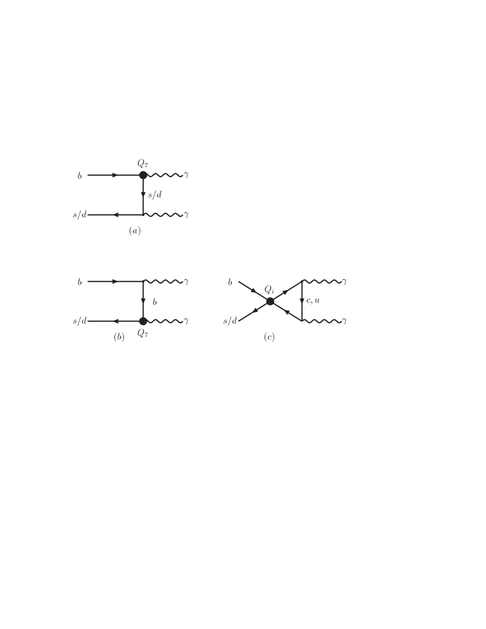
FIG. 1.: The leading power 1PR diagram (a) and subleading power 1PR diagram (b) of the magnetic penguin operator $Q_{7}$, and the subleading power 1PI diagram (c) of the four-quark operators $Q_{i}$. The diagrams with interchanged photons are not shown.

FIG. 2.: The CP violating asymmetry of $(B_{d}\to\gamma\gamma)$ decay vs the CKM angle $\gamma$ and energy scale $\mu$ in the SM. The dotted, short-dashed and solid curves show the SM predictions for $\mu=m_{b}/2,m_{b}$ and $2m_{b}$, respectively.

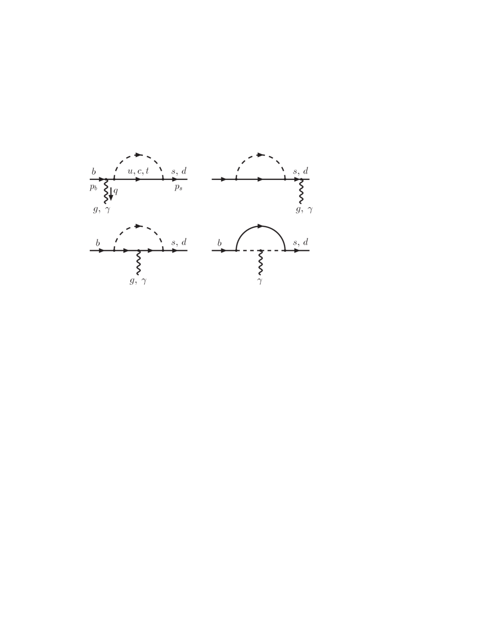
FIG. 3.: The typical photon- and gluon-penguin diagrams with W and charged-PGB exchanges (short-dashed lines) in the SM and TC2 models which contribute to $B\to X_{s,d}\gamma$ decays. The internal quarks are the upper type $u,c$ and $t$ quarks.

FIG. 4.: The branching ratios ${{\cal B}}(B\to X_{s}\gamma)$ in the SM and TC2 models as a function of $m_{\tilde{\pi}}$. The band between two horizontal dashed-lines (solid lines) shows the SM prediction (world average of experimental measurements) as listed in Eqs.(1), (2). The short-dash, solid and dot-dash curves show the TC2 model predictions of the branching ratios for $\mu=m_{b}/2,m_{b}$ and $2m_{b}$, respectively.

FIG. 5.: Plots of branching ratios ${{\cal B}}(B_{s}\to\gamma\gamma)$ (a) and ${{\cal B}}(B_{d}\to\gamma\gamma)$ (b) vs $m_{\tilde{\pi}}$, setting $\lambda_{B}=0.35$ and CKM angle $\gamma=60^{\circ}$. The lower three lines in each diagram show the SM predictions for $\mu=m_{b}/2$ (dotted line), $\mu=m_{b}$ (solid line) and $\mu=2m_{b}$ (short-dashed line). Upper three curves correspond to the theoretical predictions of TC2 model.

FIG. 6.: Plots of branching ratios ${{\cal B}}(B_{s}\to\gamma\gamma)$ (a) and ${{\cal B}}(B_{d}\to\gamma\gamma)$ (b) vs $\lambda_{B}$, setting $m_{\tilde{\pi}}=200$ GeV and CKM angle $\gamma=60^{\circ}$. The dotted and short-dashed curves show the SM predictions for $\mu=m_{b}/2$ and $\mu=m_{b}$, respectively. The dot-dashed and solid curves show the TC2 model predictions for $\mu=m_{b}/2$ and $\mu=m_{b}$, respectively.

FIG. 7.: The ratio of branching ratios $R(B_{s,d}\to\gamma\gamma)$ in the TC2 model. The three dotted and three solid curves show the ratios for $B_{s}\to\gamma\gamma$ and $B_{d}\to\gamma\gamma$ decays, respectively. In (b), we set $m_{\tilde{\pi}}=170$ GeV.

FIG. 8.: The CP violating asymmetry of $(B_{d}\to\gamma\gamma)$ decay in the SM and TC2 model. The lower (upper) dotted, short-dashed and solid curves show the SM (TC2) predictions for $\mu=m_{b}/2,m_{b}$ and $2m_{b}$, respectively.

FIG. 9.: The CP violating asymmetry of $(B_{d}\to\gamma\gamma)$ decay vs mass $m_{\tilde{\pi}}$ and energy scale $\mu$ in TC2 model. The dotted, short-dashed and solid curves show the TC2 predictions for $\mu=m_{b}/2,m_{b}$ and $2m_{b}$, respectively.

REFERENCES

• [1] G.-L. Lin, J. Liu, and Y.-P. Yao, Phys. Rev. Lett. 64, 1498 (1990); Phys. Rev. D 42, 2314 (1990); Mod. Phys. Lett. A 6, 1333 (1991); H. Simma and D. Wyler, Nucl. Phys. B 344, 283(1990); S. Herrlich and J. Kalinowski, Nucl. Phys. B 381, 501 (1992).
• [2] K.G.Chetyrkin, M.Β Misiak and M.Munz, Phys. Lett. B 400, 206(1997), ibid. B 425, 414 (E) (1998).
• [3] For more details of $B\to X_{s}\gamma$ decay, see G.Buchalla, A.J.Buras, and M.E.Lautenbacher, Rev. Mod. Phys. 68, 1125 (1996); A.J.Β Buras, in Probing the Standard Model of Particle Interactions, edited by F. David and R. Gupta (Elsevier Science B.V., Amesterdam, 1998), hep-ph/9806471.
• [4] A.L.Β Kagan and M.Β Neubert, Eur. Phys. J. C 7, 5 (1999).
• [5] For recent status of $B\to X_{s}\gamma$ decay, see M.Β Neubert, β€œRadiative B decays: Standard candles of flavor physics,” hep-ph/0212360; A.J.Β Buras, A.Β Czarnecki, M.Β Misiak, and J.Β Urban, Nucl. Phys. B 631, 219 (2002).
• [6] G.Β Hiller and E.O.Β Iltan, Phys. Lett. B 409, 425 (1997); C.-H.Β Chang, G.-L.Β Lin, and Y.-P.Β Yao, ibid., 415, 395 (1997).
• [7] G.Β Hiller, Ph.D. thesis, Hamberg University, hep-ph/9809505.
• [8] S.W.Β Bosch and G.Β Buchalla, J.High Energy Phys. 08, 054 (2002).
• [9] S.W.Β Bosch, Ph.D. thesis, Max Planck Institue, hep-ph/0208203.
• [10] D.S.Β Du, X.L.Β Li, and Z.J.Β Xiao, Phys. Rev. D 51, 279 (1995); C.D.LΓΌ and Z.J.Β Xiao, ibid 53, 2529 (1996); P.Β Singer and D.-X.Β Zhang, ibid 56, 4274 (1997); G.R.Β Lu, Z.H.Β Xiong, and Y.G.Β Cao, Nucl. Phys. B 487, 43 (1997); Z.J.Β Xiao, L.X.Β LΓΌ, H.K.Β Guo, and G.R.Β Lu, Chin. Phys. Lett. 16, 86 (1999); G.R.Β Lu, J.S.Β Huang, Z.J. Β Xiao, and C.X.Β Yue, Commun. Theor. Phys. 33, 99 (2000); Z.J.Β Xiao, L.Q.Β Jia, L.X.Β LΓΌ, and G.R.Β Lu, ibid. 33, 269 (2000).
• [11] Z.J.Β Xiao, C.S.Β Li, and K.T.Β Chao, Phys. Lett. B 473, 148 (2000); Phys. Rev. D 62, 094008 (2000); ibid. 63,074005(2001).
• [12] CLEO Collaboration, S.Β Chen et al., Phys. Rev. Lett. 87, 251807 (2001); ALEPH Collaboration, R.Β Barate et al., Phys. Lett. B 469, 129 (1998); Belle Collabloration, K.Β Abe et al., ibid. 511, 151 (2001); BaBar Collaboration, B.Β Aubert et al., β€œDetermination of the branching fraction for inclusive decays $B\to X_{s}\gamma$,” hep-ex/0207076, BaBar-Conf-02/026.
• [13] Particle Data Group, K. Hagiwara et al., Phys. Rev. D 66, 010001 (2002).
• [14] G. Hiller and E.O. Iltan, Mod. Phys. Lett. A 12, 2837 (1997); S. Choudlhury and J. Ellis, Phys. Lett. B 433, 102 (1998); W.Liu, B. Zhang, and H.Zhang, ibid. 461, 295 (1999).
• [15] T.M.Β Aliev and G.Β Turan, Phys. Rev. D 48, 1176 (1993); T.M.Β Aliev, G.Β Hiller, and E.O.Β Iltan, Nucl. Phys. B 515, 321 (1998); T.M.Β Aliev and E.O.Β Iltan, Phys. Rev. D 58, 095014 (1998).
• [16] J.J.Β Cao, Z.J.Β Xiao, and G.R.Β Lu, Phys. Rev. D 64, 014012 (2001).
• [17] S. Bertolini and J. Matias, Phys. Rev. D 57, 4197 (1998); G.G.Devidez and G.R.Jibuti, Phys. Lett. B 429, 48 (1998).
• [18] CLEO Collaboration, M.Β Acciarri et al., Phys. Lett. B 363, 137 (1995).
• [19] BaBar Collaboration, B.Β Aubert et al., Phys. Rev. Lett. 87, 241803 (2001).
• [20] C.T.Β Hill, Phys. Lett. B 345, 483 (1995).
• [21] H.Β Simma, Z. Phys. C 61, 189 (1994).
• [22] F.E.Β Low, Phys.Rev. 110, 974 (1958).
• [23] L.Β Reina, G.Β Ricciardi, and A.Β Soni, Phys. Rev. D 56, 5805 (1997).
• [24] X.G.Β He, Y.K.Β Hsiao, J.Q.Β Shi, Y.L.Β Wu, and Y.F.Β Zhou, Phys. Rev. D 64, 034002 (2001).
• [25] A.J.Β Buras and R.Β Fleischer, Eur. Phys. J. C 11, 93 (1999); Z.J.Β Xiao and M.P.Β Zhang, Phys. Rev. D 65, 114017 (2002); C.D.Β LΓΌ and Z.J.Β Xiao, ibid. 66, 074011 (2002); R.Β Fleischer, Status and prospects of CKM phase determinations, invited talk at the 8th Intern. Conf. on B Physics and Hadron Machine - BEAUTY 2002, Spain, 17-21 June 2002, hep-ex/0208083.
• [26] K.Β Lane, Phys. Rev. D 54, 2204 (1996); K.Β Lane, talk presented at the 28th International Conference on High Energy Physics, Warsaw, 1996, ICHEP 96:367-378.
• [27] S.Β Weinberg, Phys. Rev. D 13, 974 (1976); 19, 1277(1979); L.Β Susskind, ibid. 20, 2619 (1979).
• [28] E.Β Farhi and L.Β Susskind, Phys. Rev. D 20, 3404 (1979).
• [29] G.Β Buchalla, G.Β Burdman, C.T.Β Hill, and D.Β Kominis, Phys. Rev. D 53, 5185 (1996).
• [30] D.Β Kominis, Phys. Lett. B 358, 312 (1995); G.Β Burdman and D.Β Kominis, Phys. Lett. B 403, 101 (1997); G.Β Burdman, ibid. 409, 443 (1997).
• [31] E.Β Eichten, I.Β Hinchliffe, K.Β Lane, and C.Β Quigg, Rev. Mod. Phys. 56,579 (1984); Phys. Rev. D 34, 1547 (1986); E.Β Eichten and K.Β Lane, Phys. Lett. B 327, 129 (1994).
• [32] Z.J.Β Xiao, L.X.Β LΓΌ, H.K.Β Guo, and G.R.Β Lu, Eur. Phys. J. C 7, 487 (1999).
• [33] J.Β Ellis, M.K.Β Gaillard, D.V.Β Nanopoulos, and P.Β Sikivie, Nucl. Phys. B 182, 505 (1981).
• [34] Z.J.Β Xiao, C.S.Β Li, and K.T.Β Chao, Eur. Phys. J. C 10, 51 (1999).
• [35] G.Β Burdman, K.Β Lane, and T.Β Rador, Phys. Lett. B 514, 41 (2001).
• [36] Z.J.Β Xiao, W.J.Β Li, L.B.Β Guo, and G.R.Β Lu, Eur. Phys. J. C 18, 681 (2001).
• [37] P.Β Burchat et al., β€œPhysics at a $10^{36}$ asymmetric B factory,” SLAC-PUB-8970.