The Complementarity of Eastern and Western Hemisphere Long-Baseline Neutrino Oscillation Experiments

Abstract

We present a general formalism for extracting information on the fundamental parameters associated with neutrino masses and mixings from two or more long baseline neutrino oscillation experiments. This formalism is then applied to the current most likely experiments using neutrino beams from the Japan Hadron Facility (JHF) and Fermilab’s NuMI beamline. Different combinations of muon neutrino or muon anti-neutrino running are considered. To extract the type of neutrino mass hierarchy we make use of the matter effect. Contrary to naive expectation, we find that both beams using neutrinos is more suitable for determining the hierarchy provided that the neutrino energy divided by baseline ($E/L$) for NuMI is smaller than or equal to that of JHF. Whereas to determine the small mixing angle, $\theta_{13}$, and the CP or T violating phase $\delta$, one neutrino and the other anti-neutrino is most suitable. We make extensive use of bi-probability diagrams for both understanding and extracting the physics involved in such comparisons.

I Introduction

The solar neutrino puzzle, which has lasted nearly 40 years, has finally been resolved by KamLAND [1] after invaluable contributions by numerous solar neutrino experiments, especially recently by SNO[2] and Super-Kamiokande[3]. The Large-Mixing-Angle (LMA) region of the Mikheev-Smirnov-Wolfenstein (MSW) [4] triangle [5] has now been uniquely selected. This resolution to the solar neutrino puzzle has opened the door to the experimental exploration of CP violation in the Lepton Sector. Together with the existing evidence for neutrino oscillation that has been obtained by the pioneering atmospheric neutrino observations [6] and the long-baseline accelerator experiments [7], it lends further support to the standard three-flavor mixing scheme of neutrinos.

The remaining task toward the goal of uncovering the complete structure of the lepton flavor mixing would be a determination of the (1-3) sector of lepton mixing matrix which is now called as the Maki-Nakagawa-Sakata matrix (MNS)[8]. A full determination of the (1-3) sector includes a determination of $\theta_{13}$, the CP or T violating phase $\delta$ and the sign of $\Delta m^{2}_{13}$. (We define $\Delta m^{2}_{ij}\equiv m^{2}_{j}-m^{2}_{i}$, where $m_{i}$ is the mass of the $i$-th eigenstate.)

The sign of $\Delta m^{2}_{13}$ signals which pattern of neutrino masses nature has chosen, the normal hierarchy, $\Delta m^{2}_{13}>0$, or the inverted hierarchy, $\Delta m^{2}_{13}<0$. This hierarchy must certainly carry interesting information on the, yet undiscovered, underlying principle of how nature organizes the neutrino sector. While the hierarchy question is of great interest, at this moment, there is no experimental information available. One possible exception is a hint from the neutrino data from supernova SN1987A [9], however the basis of this hint is under discussion[10].

To design the experiments to measure CP or T violating phase $\delta$ we must know in advance $\theta_{13}$, or at least its order of magnitude. There have been many proposals for experiments which may be able to measure $\theta_{13}$. They can be classified into two categories, long-baseline (LBL) accelerator experiments [11, 12, 13, 14, 15], and reactor experiments [16, 17]. While $\theta_{13}$ may be eventually measured by some of these experiments it was recognized that this measurement suffers from a problem of parameter degeneracy [18, 19, 20, 21, 22, 23]. It stems from the fact that the determination of $\theta_{13}$, $\delta$ and the sign of $\Delta m^{2}_{13}$ are inherently coupled with each other.

A complete solution to the parameter degeneracy would require extensive measurement at two different energies and/or two different baselines [19, 24, 25], or to combine two different experiments [17, 25, 26, 27, 28]. We, however, seek an alternative strategy in this paper. That is, we propose to solve it one by one. We pursue the possibility that determination of the sign of $\Delta m^{2}_{13}$ may be carried out with only a limited set of measurement. It is similar in spirit to the one employed in [21] in which we proposed a way to circumvent at least partly the problem of ($\theta_{13}$, $\delta$) degeneracy.

In this paper, we explore the line of thought of comparing measurement at two different energies and/or combining two different experiments to determine the sign of $\Delta m^{2}_{13}$ and $\theta_{13}$. In particular, it is of concern to us how to combine the JHF [13] and NuMI Off-Axis [14] experiments. Apart from possibility of earlier detection in MINOS, OPERA or reactor experiments, the effect of nonzero $\theta_{13}$ is likely to be determined by observing electron appearance events in these LBL experiments. Hence, it is of great importance to uncover ways by which these two experiments can compliment one another. We discuss in this paper which combination of modes of operation ($\nu$ or $\bar{\nu}$ channels) and which neutrino energies divided by baseline ($E/L$) have better sensitivity for determining the sign of $\Delta m^{2}_{13}$ and/or measuring $\theta_{13}$.

While our treatment applies to wider context beyond application to the particular experiments, finding a way of optimizing the JHF-NuMI interplay is, we believe, a very relevant and urgent question for both of these projects. It is likely that the JHF experiment in its phase I operates in neutrino mode [13]. Given the state of the other projects, NuMI is the one which is most likely to become a reality. Therefore, it is important to find the most profitable mode of operation of the NuMI Off-Axis project.

We start by giving a general formalism of comparing two different measurement. It is to illuminate the analytic structure of the problem of two experiments comparison, and it would be of help in understanding the physical characteristics behind the observations we will provide. Instead of engaging an intensive $\chi^{2}$ analysis we prefer to illuminate the global chart of the two experiment comparison. To carry this out we rely heavily on a generalized version of the CP/T bi-probability plot that was introduced and developed in Refs. [20, 29, 23]. Our discussion in this paper, while not the complete story, it is sufficient to enable us to understand the key physics points. The experimental issues that need to be addressed to complete the picture are beyond the scope of this paper.

The reader who wants to focus on the physics conclusions, in particular on our key observations in JHF-NuMI comparison, can go directly to Sec. III, skipping Sec. II. Then, they might want to come back to read the Sec. II for a deeper understanding.

II General formalism for comparison of two different measurement

Let us combine two measurements, either $\nu$ or $\bar{\nu}$, for two different energies and/or baselines. For example, one measurement could come from JHF and another measurement from NuMI, with both $\nu$ (or $\bar{\nu}$) or one $\nu$ and the other $\bar{\nu}$. All combinations can be treated in the universal formalism presented here.

We can start with two basic equations as in [23] for small $\sin\theta_{13}$:

$$P^{\alpha}(\nu) = X^{\alpha}\theta^{2}+Y^{\alpha}\theta\cos{\left(\delta+\frac{\Delta^{\alpha}}{2}\right)}+P^{\alpha}_{\odot}$$ (1)

$$P^{\beta}(\nu) = X^{\beta}\theta^{2}+Y^{\beta}\theta\cos{\left(\delta+\frac{\Delta^{\beta}}{2}\right)}+P^{\beta}_{\odot}$$ (2)

where $\theta\equiv\sin\theta_{13}$, and the superscripts $\alpha$ and $\beta$ label the process and the experimental setup. The value of the parameters $X^{\alpha}$, $Y^{\alpha}$ and $\Delta^{\alpha}$ depend on the process (specified by $\alpha$), the energy and path length of the experiment as well as sign of $\Delta m^{2}_{13}$ and the density of matter traversed by the neutrino beam. In Table I we give the values for the $X$’s, $Y$’s and $\Delta$’s in terms of the variables $X_{\pm}$, $Y_{\pm}$ and $\Delta_{13}$ which will be defined below.

Process	$\nu_{\mu}\rightarrow\nu_{e}$	$\nu_{\mu}\rightarrow\nu_{e}$	$\bar{\nu}_{\mu}\rightarrow\bar{\nu}_{e}$	$\bar{\nu}_{\mu}\rightarrow\bar{\nu}_{e}$	$\nu_{e}\rightarrow\nu_{\mu}$	$\nu_{e}\rightarrow\nu_{\mu}$	$\bar{\nu}_{e}\rightarrow\bar{\nu}_{\mu}$	$\bar{\nu}_{e}\rightarrow\bar{\nu}_{\mu}$
sign $\Delta m^{2}_{13}$	$+$ ve	$-$ ve	$+$ ve	$-$ ve	$+$ ve	$-$ ve	$+$ ve	$-$ ve
$X$	$X_{+}$	$X_{-}$	$X_{-}$	$X_{+}$	$X_{+}$	$X_{-}$	$X_{-}$	$X_{+}$
$Y$	$Y_{+}$	$Y_{-}$	$-Y_{-}$	$-Y_{+}$	$Y_{+}$	$Y_{-}$	$-Y_{-}$	$-Y_{+}$
$\Delta$	$\Delta_{13}$	$-\Delta_{13}$	$-\Delta_{13}$	$\Delta_{13}$	$-\Delta_{13}$	$\Delta_{13}$	$\Delta_{13}$	$-\Delta_{13}$

TABLE I.: The assignments for the parameters of Eq.(2) depending on the oscillation processes and sign of $\Delta m^{2}_{13}$.

The functions $X_{\pm}$, $Y_{\pm}$ and $P_{\odot}$ are given by [30]

$$X_{\pm} = 4s^{2}_{23}\left(\frac{\Delta_{13}}{B_{\mp}}\right)^{2}\sin^{2}{\left(\frac{B_{\mp}}{2}\right)},$$ (3)

$$Y_{\pm} = \pm 8c_{12}s_{12}c_{23}s_{23}\left(\frac{\Delta_{12}}{aL}\right)\left(\frac{\Delta_{13}}{B_{\mp}}\right)\sin{\left(\frac{aL}{2}\right)}\sin{\left(\frac{B_{\mp}}{2}\right)}$$ (4)

$$P_{\odot} = c^{2}_{23}\sin^{2}{2\theta_{12}}\left(\frac{\Delta_{12}}{aL}\right)^{2}\sin^{2}{\left(\frac{aL}{2}\right)}$$ (5)

with

$$\Delta_{ij}\equiv\frac{|\Delta m^{2}_{ij}|L}{2E}\quad{\rm and}\quad B_{\pm}\equiv|\Delta_{13}\pm aL|,$$ (6)

where $a=\sqrt{2}G_{F}N_{e}$ denotes the index of refraction in matter with $G_{F}$ being the Fermi constant and $N_{e}$ a constant electron number density in the earth. Some crucial properties of the functions $X_{\pm}$ and $Y_{\pm}$ which allow this unified notation are summarized in Appendix A.

The basic equations (2) can be solved for either sign of $\Delta m^{2}_{13}$ as:

$$\theta = \sqrt{\frac{P^{\alpha}-P^{\alpha}_{\odot}}{X^{\alpha}}}-\frac{Y^{\alpha}}{2X^{\alpha}}\cos{\left(\delta+\frac{\Delta^{\alpha}}{2}\right)}~{}=~{}\sqrt{\frac{P^{\beta}-P^{\beta}_{\odot}}{X^{\beta}}}-\frac{Y^{\beta}}{2X^{\beta}}\cos{\left(\delta+\frac{\Delta^{\beta}}{2}\right)}.$$ (7)

where we have ignored terms of order $\frac{Y^{2}}{X}$. The right equality can be used to solve for both $\sin\delta$ and $\cos\delta$ from which $\theta$ is then determined. This is a straightforwardly generalization of the method used in [23] to obtain, analytically, the degenerate set of solutions and to elucidate the relationships between them. Here, we will present the result of such a general analysis in the Appendix A. An important point, however, is that once the solutions for $\delta$ are known, $\theta$ is easily obtained using left hand equality in Eq. (7).

Experimentally the most likely channels to be realized in the near future are $\nu_{\mu}\rightarrow\nu_{e}$ and $\bar{\nu}_{\mu}\rightarrow\bar{\nu}_{e}$, therefore in the next two subsections we will specialize to these channels with both beams being Neutrinos (or Anti-Neutrinos) and one beam of Neutrinos and one beam of Anti-Neutrinos. In the following section we will consider the specific experimental situations presented by the JHF[13] and NuMI[14] proposals.

A Both Neutrinos or Both Anti-Neutrinos

We apply the general formalism developed in the previous section to an explicit example of a $\nu$-$\nu$ comparison of two experiments with different energies and baseline distances. At the end of this subsection we will give the relationship to the $\bar{\nu}$-$\bar{\nu}$ comparison. We will label the two experiments J and N in reference to JHF and NuMI. However, in spite of the reference to specific two projects, our general discussions are valid for any pair of the LBL experiments on the globe and can also be used to discuss other processes but here we will concentrate on $\nu_{\mu}\rightarrow\nu_{e}$.

We start by introducing some convenient notation. Since we will treat $\Delta m^{2}_{13}>0$ and
$\Delta m^{2}_{13}<0$ simultaneously we will label the various quantities below with subscripts $\pm$ to indicate the sign of $\Delta m^{2}_{13}$. We define

$$S{\pm} \equiv \pm\frac{Y^{J}_{\pm}}{2X^{J}_{\pm}}\sin{\left(\frac{\Delta_{13}^{J}}{2}\right)}\mp\frac{Y^{N}_{\pm}}{2X^{N}_{\pm}}\sin{\left(\frac{\Delta_{13}^{N}}{2}\right)},$$ (8)

$$C_{\pm} \equiv -\frac{Y^{J}_{\pm}}{2X^{J}_{\pm}}\cos{\left(\frac{\Delta_{13}^{J}}{2}\right)}+\frac{Y^{N}_{\pm}}{2X^{N}_{\pm}}\cos{\left(\frac{\Delta_{13}^{N}}{2}\right)},$$ (9)

$$D_{\pm} \equiv S_{\pm}^{2}+C_{\pm}^{2},$$ (10)

$$\Delta P_{\pm} \equiv \sqrt{\frac{P^{J}-P^{J}_{\odot}}{X^{J}_{\pm}}}-\sqrt{\frac{P^{N}-P^{N}_{\odot}}{X^{N}_{\pm}}}.$$ (11)

The signs and the subscript assignment come from Table 1.

By solving (7) with these definitions, it is easy to derive (see Appendix A), for positive $\Delta m^{2}_{13}$, the allowed values of $(\theta,~{}\delta)$ which we assign subscripts 1 and 2;

$$\sin{\delta_{1,2}} = \frac{1}{D_{+}}\left[-S_{+}\Delta P_{+}\pm C_{+}\sqrt{D_{+}-(\Delta P_{+})^{2}}\right],$$ (12)

$$\cos{\delta_{1,2}} = \frac{1}{D_{+}}\left[-C_{+}\Delta P_{+}\mp S_{+}\sqrt{D_{+}-(\Delta P_{+})^{2}}\right].$$ (13)

Notice that with this choice of signs $\sin^{2}\delta_{i}+\cos^{2}\delta_{i}=1$. For negative $\Delta m^{2}_{13}$, we use subscripts 3 and 4 to distinguish them from the positive $\Delta m^{2}_{13}$ solutions,

$$\sin{\delta_{3,4}} = \frac{1}{D_{-}}\left[-S_{-}\Delta P_{-}\mp C_{-}\sqrt{D_{-}-(\Delta P_{-})^{2}}\right],$$ (14)

$$\cos{\delta_{3,4}} = \frac{1}{D_{-}}\left[-C_{-}\Delta P_{-}\pm S_{-}\sqrt{D_{-}-(\Delta P_{-})^{2}}\right].$$ (15)

The relative $\pm$ signs in (13) and (15) are arbitrary at this point but are the same as those used in the next subsection.

The relationships between the mixed-sign degenerate solution are given by

$$\cos{(\delta_{1}-\delta_{3})} = \frac{\left(C_{+}C_{-}+S_{+}S_{-}\right)}{D_{+}D_{-}}\left(\Delta P_{+}\Delta P_{-}-\sqrt{D_{+}-\Delta P_{+}^{2}}\sqrt{D_{-}-\Delta P_{-}^{2}}\right)$$ (16)

$$+ \frac{\left(C_{-}S_{+}-C_{+}S_{-}\right)}{D_{+}D_{-}}\left(\Delta P_{-}\sqrt{D_{+}-\Delta P_{+}^{2}}+\Delta P_{+}\sqrt{D_{-}-\Delta P_{-}^{2}}\right),$$ (17)

$$\sin{(\delta_{1}-\delta_{3})} = \frac{\left(C_{-}S_{+}-C_{+}S_{-}\right)}{D_{+}D_{-}}\left(\Delta P_{+}\Delta P_{-}-\sqrt{D_{+}-\Delta P_{+}^{2}}\sqrt{D_{-}-\Delta P_{-}^{2}}\right)$$ (18)

$$- \frac{\left(C_{+}C_{-}+S_{+}S_{-}\right)}{D_{+}D_{-}}\left(\Delta P_{-}\sqrt{D_{+}-\Delta P_{+}^{2}}+\Delta P_{+}\sqrt{D_{-}-\Delta P_{-}^{2}}\right).$$ (19)

We note that, unlike the case of $\nu$-$\bar{\nu}$ comparison [29] which will be discussed in the next section, there is no sensible limit $\Delta^{N}_{13}\rightarrow\Delta^{J}_{13}$ and $(aL)^{N}\rightarrow(aL)^{J}$ because in this limit no extra information is provided. However, one can ask the question, can we obtain some useful relationships between CP phases of the mixed-sign degeneracy in an approximation of small difference in the matter effect between JHF and NuMI? The answer is yes and we will derive such relations in Appendix B where we formulate such perturbative treatment.

The solutions for $\theta$ can easily be obtained by substituting appropriate values of $\sin\delta$ and $\cos\delta$ into Eq.(7). For positive $\Delta m^{2}_{13}$, the values of $\theta_{1,2}$ are obtained by using the $X^{J}_{+},~{}Y^{J}_{+},~{}\Delta^{J}_{13}$ and $X^{N}_{+},~{}Y^{N}_{+},~{}\Delta^{N}_{13}$ in Eq.(7) and for negative $\Delta m^{2}_{13}$, the values of $\theta_{3,4}$ are obtained by using $X^{J}_{-},~{}Y^{J}_{-},~{}-\Delta^{J}_{13}$ and $X^{N}_{-},~{}Y^{N}_{-},~{}-\Delta^{N}_{13}$. See Eq.(53) of the Appendix A for explicit expressions.

For the $\bar{\nu}$-$\bar{\nu}$ comparison: for positive $\Delta m^{2}_{13}$, the values of $\theta_{1,2}$ are obtained by using the $X^{J}_{-},~{}-Y^{J}_{-},~{}-\Delta^{J}_{13}$ and $X^{N}_{-},~{}-Y^{N}_{-},~{}-\Delta^{N}_{13}$ in Eq.(7) and for negative $\Delta m^{2}_{13}$, the values of $\theta_{3,4}$ are obtained by using $X^{J}_{+},~{}-Y^{J}_{+},~{}\Delta^{J}_{13}$ and $X^{N}_{+},~{}-Y^{N}_{+},~{}\Delta^{N}_{13}$. Thus the allowed region for the $\bar{\nu}$-$\bar{\nu}$ comparison is identical to the $\nu$-$\nu$ comparison except for the fact that the roles of $\Delta m^{2}_{13}>0$ and $\Delta m^{2}_{13}<0$ are interchanged.

B One Neutrinos, One Anti-Neutrinos

We want to treat the $\nu$-$\bar{\nu}$ comparison in an entirely analogous fashion as the $\nu$-$\nu$ comparison in the previous subsection. Toward this goal we introduce a similar notation:

$$S^{\prime}_{\pm} \equiv \pm\frac{Y^{J}_{\pm}}{2X^{J}_{\pm}}\sin{\left(\frac{\Delta_{13}^{J}}{2}\right)}\mp\frac{Y^{N}_{\mp}}{2X^{N}_{\mp}}\sin{\left(\frac{\Delta_{13}^{N}}{2}\right)},$$ (20)

$$C^{\prime}_{\pm} \equiv -\frac{Y^{J}_{\pm}}{2X^{J}_{\pm}}\cos{\left(\frac{\Delta_{13}^{J}}{2}\right)}-\frac{Y^{N}_{\mp}}{2X^{N}_{\mp}}\cos{\left(\frac{\Delta_{13}^{N}}{2}\right)},$$ (21)

$$D^{\prime}_{\pm} \equiv (S^{\prime}_{\pm})^{2}+(C^{\prime}_{\pm})^{2},$$ (22)

$$\Delta P^{\prime}_{\pm} \equiv \sqrt{\frac{P^{J}-P^{J}_{\odot}}{X^{J}_{\pm}}}-\sqrt{\frac{P^{N}-P^{N}_{\odot}}{X^{N}_{\mp}}}.$$ (23)

where the subscript $\pm$ in (23) denote the sign of $\Delta m^{2}_{13}$ and here $P^{N}$ is for anti-neutrinos. The signs and the subscript assignment come from Table 1. These definitions are almost identical to the $\nu$-$\nu$ definitions but not quite, the $\pm$ labels on the left hand side are different and these difference lead to markedly different outcomes.

It is easy to verify that by using the above notation $\sin{\delta_{i}}$ as well as $\theta_{i}$ are given by exactly the same expressions as in the previous sections, e.g., (13) and (15), apart from replacement $S_{\pm}\rightarrow S^{\prime}_{\pm}$, $C_{\pm}\rightarrow C^{\prime}_{\pm}$, and so on.

The relative $\pm$ signs in (13) and (15) are determined such that it reproduces the pair of the degenerate solutions, $\delta_{3}=\delta_{1}+\pi$ (mod. $2\pi$) in the limit of $P^{N}=P^{J}$, $\Delta^{J}=\Delta^{N}$ and $(aL)^{J}=(aL)^{N}$ for a given value of $\theta_{13}$ [23]. The relation, however, receives corrections due to difference in matter effect between JHF and NuMI even at $\Delta^{J}=\Delta^{N}$. It is not difficult to compute the correction at $P^{N}=P^{J}$ in the form

$$\delta_{3}=\delta_{1}+\pi+C^{N-J}\left[(aL)^{N}-(aL)^{J}\right],$$ (24)

to first order in JHF-NuMI difference of matter effects. The coefficient $C^{N-J}$ is given in Appendix B.

Notice that the relation between the same-sign solutions of the CP violating phase is given generically by the formula (57) in comparison of any two channels. Among other things, $\delta_{2}=\pi-\delta_{1}$ always holds at oscillation maximum, $\Delta^{N}=\Delta^{J}=\pi$, despite the difference in matter effects at JHF and NuMI. It must be the case since the bi-probability trajectories shrink to straight lines.

III JHF verses NuMI Comparison

In this section we will discuss explicitly the JHF and NuMI possibilities. JHF will have a baseline of 295km, and the neutrino energy at which oscillation maximum occurs is

$$0.60~{}\text{GeV}\left({\Delta m^{2}_{13}\over 2.5\times 10^{-3}~{}eV^{2}}\right).$$ (25)

For our figures we will use this energy plus 0.8 GeV which is 33% higher and near the peak in the event rate for $\nu_{e}$ appearance due to the rising cross section but falling oscillation probability assuming the same flux can be maintained.

So far the path length for NuMI is undecided but it will most likely be between 500 and 1000 km. We use 732km for our figures, the path length of NuMI/MINOS. At this distance oscillation maximum occurs at

$$1.5~{}\text{GeV}\left({\Delta m^{2}_{13}\over 2.5\times 10^{-3}~{}\text{eV}^{2}}\right)\left({L\over 732~{}\text{km}}\right).$$ (26)

The other energy used is 33% higher at 2.0 GeV near the event rate peak for the reasons stated for JHF.

In Fig. 1 we have plotted the allowed region in bi-probability space assume no knowledge of $\theta$ and $\delta$ in a comparison between JHF neutrinos and NuMI neutrinos. This allowed region forms two narrow “pencils” which originate at the origin and grow in width away from the origin. Associated with each of these “pencils” is the sign of $\Delta m^{2}_{13}$, thus if the pencils are well separated then a comparison of these two experiments can be used to determine the sign of $\Delta m^{2}_{13}$. But the size of $\theta_{13}$ is poorly determined in such a comparison. More details on this $\nu$-$\nu$ comparison will be given in the next subsection. (A $\bar{\nu}$-$\bar{\nu}$ comparison is identical but with the sign of $\Delta m^{2}_{13}$ flipped.)

In Fig. 2 we have plotted the allowed region in bi-probability space in a comparison between JHF neutrinos and NuMI anti-neutrinos. Here the allowed regions are very broad and there is significant overlap between the allowed regions for the two signs of $\Delta m^{2}_{13}$. However, the size of $\theta_{13}$ can be determined with reasonable accuracy in such a comparison. Fig. 3 is similar to Fig. 2 but here the concentration is on the overlap region. More details of this $\nu$-$\bar{\nu}$ will be given in the subsection following the $\nu$-$\nu$ comparison. (A $\bar{\nu}$-$\nu$ comparison is identical to a $\nu$-$\bar{\nu}$ but with the sign of $\Delta m^{2}_{13}$ flipped.)

A Both Neutrinos

It is worthwhile to have a simple formula which relates between two $\nu_{\mu}\rightarrow\nu_{e}$ appearance probabilities obtained by JHF and NuMI both in neutrino (or anti-neutrino) channel. Let us restrict, for definiteness, the following discussion into the case of neutrino channel. Then, one can easily derive the following expression

$$\frac{P^{N}-P^{N}_{\odot}}{X^{N}_{\pm}}-\frac{P^{J}-P^{J}_{\odot}}{X^{J}_{\pm}} = ~{}~{}\left[\frac{Y^{N}_{\pm}}{X^{N}_{\pm}}\cos{\left(\frac{\Delta_{13}^{N}}{2}\right)}-\frac{Y^{J}_{\pm}}{X^{J}_{\pm}}\cos{\left(\frac{\Delta_{13}^{J}}{2}\right)}\right]\theta\cos{\delta}$$ (28)

$$-\left[\frac{Y^{N}_{\pm}}{X^{N}_{\pm}}\sin{\left(\frac{\Delta_{13}^{N}}{2}\right)}-\frac{Y^{J}_{\pm}}{X^{J}_{\pm}}\sin{\left(\frac{\Delta_{13}^{J}}{2}\right)}\right]\theta\sin{\delta}$$

$$= 2\left(C_{\pm}\cos{\delta}\pm S_{\pm}\sin{\delta}\right)\theta$$ (29)

We want to understand the behavior of two loci corresponding to positive and negative $\Delta m^{2}_{13}$ in Fig. 1 as a function of $\Delta^{J}$ and $\Delta^{N}$. In particular, we are interested in how the slopes of the two “pencils” change in Fig. 1. To this goal we compute the slope ratio of the central axis of positive $\Delta m^{2}_{13}$ to the negative $\Delta m^{2}_{13}$. Since the central axis of the “pencil” is obtained by equating LHS of Eq. (29) to zero, the slope of $P^{N}-P^{J}$ line in Fig. 1 is simply given by $\alpha_{\pm}\equiv\frac{X^{N}_{\pm}}{X^{J}_{\pm}}$. Thus the slope ratio can be written as

$$\frac{\alpha_{+}}{\alpha_{-}}=\frac{\frac{X^{N}_{+}}{X^{N}_{-}}}{\frac{X^{J}_{+}}{X^{J}_{-}}}=\frac{\sin^{2}{\left(\frac{B_{-}^{N}}{2}\right)}/(\frac{B_{-}^{N}}{2})^{2}}{\sin^{2}{\left(\frac{B_{+}^{N}}{2}\right)}/(\frac{B_{+}^{N}}{2})^{2}}\times\frac{\sin^{2}{\left(\frac{B_{+}^{J}}{2}\right)}/(\frac{B_{+}^{J}}{2})^{2}}{\sin^{2}{\left(\frac{B_{-}^{J}}{2}\right)}/(\frac{B_{-}^{J}}{2})^{2}}$$ (30)

Therefore, the behavior of the slope ratio is controlled by a single function $\sin^{2}{x}/x^{2}$.

To have a qualitative understanding we perform perturbation expansion assuming matter effect is small, $aL\ll\Delta_{13}$. Noting that $B_{\pm}=\Delta_{13}\pm aL$ for both JHF and NuMI we obtain, to first order in matter effect,

$$\frac{\alpha_{+}}{\alpha_{-}}=1+2\left[\frac{2}{\Delta_{13}^{N}}-\cot{\left(\frac{\Delta_{13}^{N}}{2}\right)}\right](aL)|_{NuMI}-2\left[\frac{2}{\Delta_{13}^{J}}-\cot{\left(\frac{\Delta_{13}^{J}}{2}\right)}\right](aL)|_{JHF}$$ (31)

Therefore, the slope of positive-$\Delta m^{2}_{13}$ “pencil” is larger than negative-$\Delta m^{2}_{13}$ “pencil” because of the larger matter effect in NuMI.

To understand the energy dependence of the slope ratio we note that $\frac{1}{x}-\cot{x}$ is a monotonically increasing function of $x$ in $0\leq x\leq\pi$. Let us first examine the case of $\Delta_{13}^{N}=\Delta_{13}^{J}$. When the neutrino energy is increased from the oscillation maximum (which means lowering $\Delta_{13}$’s) the slope ratio decreases, in agreement with the behavior in Fig. 1, from 1(a) to 1(d). We have checked that lowering the energy (larger $\Delta_{13}$’s) in fact leads to larger slope ratio. However at energies below oscillation maximum the probabilities and event rates rapidly get smaller.

The behavior of slopes of “pencils” in other parts in Fig. 1 can also be understood in a similar manner. From Fig. 1(a) to 1(b) the slope ratio decreases, whereas from Fig. 1(a) to 1(c) it increases. The change in 1(a) to 1(b) is obtained by lowering $\Delta_{13}^{N}$ while keeping $\Delta_{13}^{J}$ fixed. Since the second term in the RHS of (31) decreases as $\Delta_{13}^{N}$ decreases, and hence the slope ratio decreases, in agreement with Figs. 1(a) and 1(b). Similarly, from Fig. 1(a) to 1(c) $\Delta_{13}^{J}$ decreases while keeping $\Delta_{13}^{N}$ is kept fixed. It should lead relatively small amount of increase in the slope ratio, again in agreement with Figs. 1(a) and 1(c).

However the slope of these “pencils” is not the total story, the width of the “pencils” is also important. Although the ratio of slopes is slightly larger in Fig. 1(c) than Fig. 1(a) the width of the “pencils” is significantly larger for Fig. 1(c) than Fig. 1(a) such that the separation of the allowed regions is smaller for Fig. 1(c) than Fig. 1(a). The square of the width of the “pencils” is controlled by the quantity

$$4(S_{\pm}^{2}+C_{\pm}^{2}) = \left(\frac{Y^{N}_{\pm}}{X^{N}_{\pm}}\right)^{2}+\left(\frac{Y^{J}_{\pm}}{X^{J}_{\pm}}\right)^{2}-2\left(\frac{Y^{N}_{\pm}}{X^{N}_{\pm}}\right)\left(\frac{Y^{J}_{\pm}}{X^{J}_{\pm}}\right)\cos(\frac{\Delta^{N}_{13}}{2}-\frac{\Delta^{J}_{13}}{2}).$$ (32)

For $\Delta^{N}_{13}=\Delta^{J}_{13}$, the width equals

$$\left(\frac{Y^{N}_{\pm}}{X^{N}_{\pm}}\right. - \left.\frac{Y^{J}_{\pm}}{X^{J}_{\pm}}\right)^{2},$$ (33)

and is very small. This smallness follows from the fact that, at the same $\Delta_{13}$, the identity $\frac{Y^{N}_{\pm}}{\sqrt{X^{N}_{\pm}}}=\frac{Y^{J}_{\pm}}{\sqrt{X^{J}_{\pm}}}$ holds ( $\frac{Y}{\sqrt{X}}$ depends only on vacuum parameters), and ratio of $X^{N}_{\pm}$ to ${X^{J}_{\pm}}$ is close to unit. If $\Delta^{N}_{13}\neq\Delta^{J}_{13}$, then $\frac{Y^{N}_{\pm}}{\sqrt{X^{N}_{\pm}}}\neq\frac{Y^{J}_{\pm}}{\sqrt{X^{J}_{\pm}}}$ and the width of the pencil grows rapidly as the cancellation that occurs for the same $\Delta_{13}$ no longer holds. Thus the width of the “pencils” in Fig. 1(b) and Fig. 1(c) are approximately equal and are much larger than the width in Fig. 1(a) and Fig. 1(d).

The conclusion to be gained from these results and figures is that if you are making a comparison of a JHF neutrino experiment and a NuMI neutrino experiment to determine the sign $\Delta m^{2}_{13}$ then the best separation occurs when $\Delta^{J}=\Delta^{N}$ i.e. the same $\frac{E}{L}$ for both experiments. Smaller values of the $E$ are slightly preferred so that we expect the optimum value, once all experimental issues are included, to be near oscillation maximum (Fig. 1(a) and 1(d)). Away from the same $\frac{E}{L}$ for both experiments the separation between the allowed region becomes worse, apart from special ranges of the CP or T violating phase $\delta$ when $\left(\frac{E}{L}\right)|_{JHF}>\left(\frac{E}{L}\right)|_{NuMI}$ (Fig. 1(c)). Whereas for the choice $\left(\frac{E}{L}\right)|_{JHF}<\left(\frac{E}{L}\right)|_{NuMI}$ (i.e $\Delta^{J}>\Delta^{N}$) there is significant overlap between the two different sign of $\Delta m^{2}_{13}$ allowed regions (Fig. 1(b)). (If one moves further, say, to $E_{JHF}=0.6$ GeV and $E_{NuMI}=2.5$ GeV, the two pencils overlap almost completely.) In these regions no matter how accurate the experiment the sign of $\Delta m^{2}_{13}$ cannot be determined by this comparison. (For JHF anti-neutrinos versus NuMI anti-neutrinos the conclusion is the same.)

In summary, for the comparison JHF neutrinos to NuMI neutrinos to be useful in the determination of the sign of $\Delta m^{2}_{13}$, choosing

$$\left(\frac{E}{L}\right)|_{JHF}\geq\left(\frac{E}{L}\right)|_{NuMI}$$ (34)

is of great importance with the preference for equal $\left(\frac{E}{L}\right)$. For $\left(\frac{E}{L}\right)|_{JHF}<\left(\frac{E}{L}\right)|_{NuMI}$ there is significant overlap between the narrow allowed regions so that this is not a good choice for this comparison.

Contrary to advantage of $\nu$-$\nu$ comparison in determination of the sign of $\Delta m^{2}_{13}$, measurement of $\theta_{13}$ suffers from large uncertainty in this channel. The bi-probalitity trajectory, for a given $\theta$, moves nearly along the direction of the “pencil” as one varies $\delta$, thus any measurement of the oscillation probabilities with finite resolution cannot pinpoint the value of $\theta$. To indicate this point we have plotted in Fig. 1 by numbers in % beside thin arcs the fractional difference $\Delta\theta/\theta\equiv(\theta_{2}-\theta_{1})/\left((\theta_{2}+\theta_{1})/2\right)$, where $\theta_{2}$ and $\theta_{1}$ here indicate the maximal and the minimal values of $\theta_{13}$ along each arc. The numbers are large, typically 30 % or even larger.

In fact, it is easy to do analytical estimate of the fractional difference. Suppose that we have measured an appearance probability $P^{J}$ or $P^{N}$. We assume for simplicity that we know the sign of $\Delta m^{2}_{13}$, and restrict ourselves into the case of oscillation maximum, $\Delta^{J}_{13}=\Delta^{N}_{13}=\pi$. The measured probability allows a range of $\theta_{13}$ [21] and one can easily calculate the maximal value of $\Delta\theta/\theta$ within the range, which leads to

$$\frac{\Delta\theta}{\theta}=\sin{2\theta_{12}}c_{23}\frac{\Delta_{12}}{\sqrt{P^{J/N}}}\left(\frac{\sin{(aL/2)}}{aL/2}\right).$$ (35)

Since $P^{J/N}$ is a few % level, it leads to a few tens in % of the fractional difference, in agreement with the numbers in Fig. 1.

B One Neutrinos and One Anti-Neutrinos

We now turn to the comparison for JHF neutrinos and NuMI anti-neutrinos or vice versa with flipped signs of $\Delta m^{2}_{13}$. Again one can write a simple formulae relating the two oscillation probabilities similar to Eq. (29)

$$\frac{P^{N}-P^{N}_{\odot}}{X^{N}_{\mp}}-\frac{P^{J}-P^{J}_{\odot}}{X^{J}_{\pm}} = ~{}~{}\left[\frac{-Y^{N}_{\mp}}{X^{N}_{\mp}}\cos{\left(\frac{\Delta_{13}^{N}}{2}\right)}-\frac{Y^{J}_{\pm}}{X^{J}_{\pm}}\cos{\left(\frac{\Delta_{13}^{J}}{2}\right)}\right]\theta\cos{\delta}$$ (37)

$$-\left[\frac{Y^{N}_{\mp}}{X^{N}_{\mp}}\sin{\left(\frac{\Delta_{13}^{N}}{2}\right)}-\frac{Y^{J}_{\pm}}{X^{J}_{\pm}}\sin{\left(\frac{\Delta_{13}^{J}}{2}\right)}\right]\theta\sin{\delta}$$

$$= 2\left(C_{\pm}\cos{\delta}\pm S_{\pm}\sin{\delta}\right)\theta$$ (38)

The square of the RHS of this equation controls the square of the width of the allowed region and is given by

$$4(S_{\pm}^{2}+C_{\pm}^{2}) = \left(\frac{Y^{N}_{\mp}}{X^{N}_{\mp}}\right)^{2}+\left(\frac{Y^{J}_{\pm}}{X^{J}_{\pm}}\right)^{2}+2\left(\frac{Y^{N}_{\mp}}{X^{N}_{\mp}}\right)\left(\frac{Y^{J}_{\pm}}{X^{J}_{\pm}}\right)\cos(\frac{\Delta^{N}_{13}}{2}+\frac{\Delta^{J}_{13}}{2})$$ (39)

apart from an overall factor of $\theta^{2}$. As $(\Delta^{N}_{13}+\Delta^{J}_{13})$ varies from $\pi$ (both experiments at energies twice the oscillation maximum energy) to $2\pi$ (both experiments at the oscillation maximum energy) this squared width grows from

$$\left(\frac{Y^{N}_{\mp}}{X^{N}_{\mp}}\right)^{2}+\left(\frac{Y^{J}_{\pm}}{X^{J}_{\pm}}\right)^{2}\quad {\rm to} \quad\left(\frac{Y^{N}_{\mp}}{X^{N}_{\mp}}\right.-\left.\frac{Y^{J}_{\pm}}{X^{J}_{\pm}}\right)^{2}.$$ (40)

Note that the later width is larger than the first width since $Y_{-}/X_{-}$ has opposite sign to $Y_{+}/X_{+}$ (no cancellation occurs here). Thus the width of the allowed region grows as you lower the energies of the experiments to oscillation maximum. This can be seen in Fig. 2; 2(d) has the smallest width whereas 2(a) has the largest in accordance with the above statement.

There is significant overlap between the allowed regions of positive and negative $\Delta m^{2}_{13}$ contours. Hence, the $\nu$-$\bar{\nu}$ comparison does not appear to be the right way for determining the sign, unless $\delta$ turns out to be close to $3\pi/2$ and $\pi/2$ for $\Delta m^{2}_{13}>0$ and $\Delta m^{2}_{13}<0$ cases, respectively [20]. However, this comparison may be better to measure $\theta_{13}$ if JHF operate only in neutrino channel, as planned, and if NuMI Off-Axis is running with significant overlap with JHF phase I. For this purpose, the best way of measuring $\theta_{13}$ would be to tune the energy at oscillation maxima for both JHF and NuMI. This is just an extension of the KMN strategy[21].

The reader may be curious as to why the slopes of the shrunken trajectories at $\Delta_{13}=\pi$ are positive in $\nu$-$\nu$ comparison whereas they are negative in $\nu$-$\bar{\nu}$ comparison. This can be easily understood as follows: The slopes of shrunken trajectories in $\nu$-$\nu$ comparison are given by $Y^{N}_{+}/Y^{J}_{+}$ ($Y^{N}_{-}/Y^{J}_{-}$) for positive (negative) $\Delta m^{2}_{13}$. On the other hand, the slopes in $\nu$-$\bar{\nu}$ comparison are given by $Y^{N}_{-}/Y^{J}_{+}$ ($Y^{N}_{+}/Y^{J}_{-}$) for positive (negative) $\Delta m^{2}_{13}$. Since $Y_{\pm}$ differ in sign, as in Eq. (4), the latter slopes are negative definite, whereas the former are positive definite. The fact that the $\nu$-$\nu$ trajectory is along the “pencil” and $\nu$-$\bar{\nu}$ trajectory is perpendicular to axis of the “cigar” can be understood by a similar argument.

IV Another Interesting Comparison

When we have access to $\nu_{e}$ and $\bar{\nu}_{e}$ beams then a comparison of a $\nu_{\mu}\rightarrow\nu_{e}$ experiment with $\bar{\nu}_{e}\rightarrow\bar{\nu}_{\mu}$ experiment will be possible. This comparison is interesting because it directly compares two CPT conjugate processes. If CPT is conserved, then at the same E/L the only difference between the oscillation probabilities for $\nu_{\mu}\rightarrow\nu_{e}$ and $\bar{\nu}_{e}\rightarrow\bar{\nu}_{\mu}$ can come from matter effects. Thus this comparison is even more sensitive to the mass hierarchy, i.e. the sign of $\Delta m^{2}_{13}$, than the neutrino-neutrino comparison discussed earlier in the previous section.

For this comparison the bi-probability figure looks similar to Fig. 1 but the difference in slope between the “pencils” is enhanced because the sign of the matter effect is opposite for $\bar{\nu}_{e}\rightarrow\bar{\nu}_{\mu}$ compared to $\nu_{\mu}\rightarrow\nu_{e}$ and the CP or T violating terms are identical in sign and magnitude. Therefore this comparison provides an excellent way to separate the two signs of $\Delta m^{2}_{13}$. If we label the two experiments as J and N as before then the ratio of slopes is given by

$$\frac{\alpha_{+}}{\alpha_{-}}=\frac{\frac{X^{N}_{+}}{X^{N}_{-}}}{\frac{X^{J}_{-}}{X^{J}_{+}}} = 1+2\left[\frac{2}{\Delta_{13}^{N}}-\cot{\left(\frac{\Delta_{13}^{N}}{2}\right)}\right](aL)|_{N}+2\left[\frac{2}{\Delta_{13}^{J}}-\cot{\left(\frac{\Delta_{13}^{J}}{2}\right)}\right](aL)|_{J}.$$ (41)

This expression differs from that of Eq.(31) by the sign of the third term. Here the matter effects for both experiments enhance the ratio of the slopes whereas in the neutrino-neutrino comparison early there was a partial cancellation. Although at present the comparison of this section is purely academic it is instructive and useful for understanding the general nature of the comparison of neutrino oscillation experiments and will be important to test the possibility of CPT violation in the future.

V Summary and Conclusions

We have presented a general formalism for comparing two or more long baseline neutrino oscillation experiments and applied this formalism to the JHF and NuMI experiments. The combination of modes that will be important depends on the question one is asking and what other information is available at the time. The use of bi-probability diagrams like the ones presented in this paper will be important for understanding the physics issues and making trade offs at the time decisions are made regarding neutrino energies and modes of operation.

In general, the both neutrino or both anti-neutrino comparison is useful for determining whether the mass hierarchy is normal or inverted, i.e. the sign $\Delta m^{2}_{13}$. However, it is important here that the experiment with the larger matter effect (longer baseline - NuMI) have a smaller or equal neutrino energy over baseline, E/L, than the experiment with smaller matter effect (shorter baseline - JHF). If the JHF experiment runs first then NuMI should also run at a similar or smaller E/L to provide the best sensitivity to the different mass hierarchies. The separation between the different mass hierarchies is reduced if the NuMI E/L is higher than the JHF E/L. The size of the small mixing angle, $\theta_{13}$, cannot be determined to better than about 30% with this comparison alone.

The one neutrino - one anti-neutrino comparison is in general most useful for determining the size of the small mixing angle, $\theta_{13}$ and the CP or T violating phase $\delta$. It could also be useful in determining the mass hierarchy provided nature does not choose the large overlap region in the bi-probability plot. For this comparison, the uncertainty in $\theta_{13}$ from the degeneracy issue is not important until the experimental resolution in $\theta_{13}$ is better than 10%.

Appendix A

In this Appendix, we first explain briefly why the universal formalism with generic notations given in Table 1 is possible. The first secret behind it is the relationship between $X$’s and $Y$’s with different sign of $\Delta m^{2}_{13}$. Let us think of the expressions of the appearance probabilities in neutrino and anti-neutrino channel similar to (2), and define coefficient function $\bar{X}_{\pm}$ as well as $X_{\pm}$. They can be expressed by using a single function $X$ as $X_{\pm}\equiv X(\pm\Delta m^{2},a)$ and $\bar{X}_{\pm}=X(\pm\Delta m^{2},-a)$. The similar notation can also be defined for $Y$’s. Then,

$$X_{\pm} = \bar{X}_{\mp}$$ (42)

$$Y_{\pm} = -\bar{Y}_{\mp},$$ (43)

because $X$’s and $Y$’s (except for extra sign) are the function only of $\Delta_{13}\pm aL$, which follows from the CP-CP relation in [29] and the approximation introduced in [30]. We note that $X_{\pm}$ and $Y_{\pm}$ satisfy the useful identity

$${Y_{+}\over\sqrt{X_{+}}}=-~{}{Y_{-}\over\sqrt{X_{-}}}.$$ (44)

Next we present general solutions of (2) whose validity extends any combinations of channels tabulated in Table 1. For any given process and sign of $\Delta m^{2}_{13}$ there are two solutions to these equations which we will label by $(\theta_{1},\delta_{1})$ and $(\theta_{2},\delta_{2})$. The equations (7) can be solved for the CP phase $\delta$ for either sign of $\Delta m^{2}_{13}$ as:

$$\sin{\delta_{1,2}} = \left[-S\Delta P\pm C\sqrt{S^{2}+C^{2}-(\Delta P)^{2}}\right]/(S^{2}+C^{2})$$ (45)

$$\cos{\delta_{1,2}} = \left[-C\Delta P\mp S\sqrt{S^{2}+C^{2}-(\Delta P)^{2}}\right]/(S^{2}+C^{2})$$ (46)

Notice that with this choice of signs $\sin^{2}\delta_{i}+\cos^{2}\delta_{i}=1$, and the variables $\Delta P$, $S$, and $C$ are defined as

$$\Delta P \equiv \sqrt{\frac{P^{\alpha}-P^{\alpha}_{\odot}}{X^{\alpha}}}-\sqrt{\frac{P^{\beta}-P^{\beta}_{\odot}}{X^{\beta}}}$$ (47)

$$S \equiv \left[R^{\alpha}\sin{\left(\frac{\Delta^{\alpha}}{2}\right)}-R^{\beta}\sin{\left(\frac{\Delta^{\beta}}{2}\right)}\right]$$ (48)

$$C \equiv \left[-R^{\alpha}\cos{\left(\frac{\Delta^{\alpha}}{2}\right)}+R^{\beta}\cos{\left(\frac{\Delta^{\beta}}{2}\right)}\right],$$ (49)

where we have defined the variable

$$R^{\alpha} \equiv \frac{Y^{\alpha}}{2X^{\alpha}}$$ (50)

which appears frequently. The corresponding $\theta$’s are then given by

$$\theta_{1,2} = \left(R^{\alpha}\sin{(\frac{\Delta^{\alpha}}{2})}\sqrt{\frac{(P^{\beta}-P^{\beta}_{\odot})}{X^{\beta}}}-R^{\beta}\sin{(\frac{\Delta^{\beta}}{2})}\sqrt{\frac{(P^{\alpha}-P^{\alpha}_{\odot})}{X^{\alpha}}}\right.$$ (53)

$$+\left.R^{\alpha}\sin{(\frac{\Delta^{\alpha}}{2})}R^{\beta}\sin{(\frac{\Delta^{\beta}}{2})}\left(\cot{\frac{\Delta^{\alpha}}{2}}-\cot{\frac{\Delta^{\beta}}{2}}\right)\cos{\delta_{1,2}}\right)$$

$$/\left({R^{\alpha}\sin{(\frac{\Delta^{\alpha}}{2})}-R^{\beta}\sin{(\frac{\Delta^{\beta}}{2})}}\right).$$

Under the interchange of $\alpha$ and $\beta$, $\delta_{1}\leftrightarrow\delta_{2}$ and $\theta_{1}\leftrightarrow\theta_{2}$ as it should. Also for useful experiments $\cot{\frac{\Delta^{\alpha}}{2}}$ is always finite. These two solutions coincide, $\theta_{1}=\theta_{2}$, when the coefficient in front of the $\cos\delta_{1,2}$ term vanishes or $\cos\delta_{1}=\cos\delta_{2}$. The first possibility occurs when $\Delta^{\alpha}=\Delta^{\beta}$ or $\Delta^{\alpha}=\pm\pi=\pm\Delta^{\beta}$. While the second occurs at the edge of the allowed region when the square root in Eq.(46) vanishes.

The allowed region in $(P^{\beta},P^{\alpha})$ bi-probability space is given by

$$(\Delta P)^{2} \leq S^{2}+C^{2}={(R^{\alpha})^{2}+(R^{\beta})^{2}-2R^{\alpha}R^{\beta}\cos{\left(\frac{\Delta^{\alpha}}{2}-\frac{\Delta^{\beta}}{2}\right)}}.$$ (54)

This region is determined by requiring the $\sin\delta$ and $\cos\delta$ to be real. The boundary is determined by the equality in eqn (54). Thus the quantity

$$(R^{\alpha})^{2}+(R^{\beta})^{2} - 2R^{\alpha}R^{\beta}\cos{\left(\frac{\Delta^{\alpha}}{2}-\frac{\Delta^{\beta}}{2}\right)}.$$ (55)

controls the separation of the two boundaries and hence the size of the allowed region. Depending on the value of $(\Delta^{\alpha}-\Delta^{\beta})$ this can range from $(\Delta P)^{2}=(R^{\alpha}-R^{\beta})^{2}$ when $(\Delta^{\alpha}-\Delta^{\beta})=0,~{}2\pi\cdots$ to $(\Delta P)^{2}=(R^{\alpha}+R^{\beta})^{2}$ for $(\Delta^{\alpha}-\Delta^{\beta})=\pm\pi,\pm 3\pi\cdots$. Which of these two extremes gives the larger allowed region depends on the relative signs of $R^{\alpha}$ and $R^{\beta}$. This will be very important since the relative signs changes as we go from both neutrino (or both anti-neutrino) to one neutrino and one anti-neutrino process.

Let us now compute the difference between two solutions of $\delta$. One can show by using (46) that

$$\cos{(\delta_{1}+\delta_{2})} = 1-2\frac{\left[R^{\alpha}\sin{\left(\frac{\Delta^{\alpha}}{2}\right)}-R^{\beta}\sin{\left(\frac{\Delta^{\beta}}{2}\right)}\right]^{2}}{(R^{\alpha})^{2}+(R^{\beta})^{2}-2R^{\alpha}R^{\beta}\cos{\left(\frac{\Delta^{\alpha}}{2}-\frac{\Delta^{\beta}}{2}\right)}}.$$ (56)

One can easily check that Eq. (56) reduces to Eq. (45) of [23] if we take $\Delta^{\alpha}=-\Delta^{\beta}$. The relationship (56) implies that

$$\delta_{2} = \pi-\delta_{1}+2\arcsin{\frac{|R^{\alpha}\sin{\left(\frac{\Delta^{\alpha}}{2}\right)}-R^{\beta}\sin{\left(\frac{\Delta^{\beta}}{2}\right)}|}{\sqrt{(R^{\alpha})^{2}+(R^{\beta})^{2}-2R^{\alpha}R^{\beta}\cos{\left(\frac{\Delta^{\alpha}}{2}-\frac{\Delta^{\beta}}{2}\right)}}}}$$ (57)

where use has been made of the relation $\arccos{(1-2x^{2})}=2\arcsin{x}$. Thus the second solution $\delta_{2}$ differs from $\pi-\delta_{1}$ by a constant which depends on the energy and path length of the neutrino beams as well as on the process but not on the mixing angle $\theta_{13}$ for any two-experiment comparison. This generalizes the result obtained in [23].

At the oscillation maximum, $|\Delta^{\alpha}|=|\Delta^{\beta}|=\pi$ and $\cos{(\delta_{1}+\delta_{2})}=-1$ i.e $\delta_{2}=\pi-\delta_{1}$. This is a reflection on the fact that at oscillation maximum the trajectory in the bi-probability space is an ellipse with zero width as can easily be seen from Eq. (2) as there is no dependence on $\cos\delta$ at this point.

Appendix B

We evaluate the correction to the relationship between two degenerate solutions of $\delta$ in $\nu$-$\nu$ and $\nu$-$\bar{\nu}$ comparison. Let us first discuss $\nu$-$\bar{\nu}$ comparison first.

We expand $S^{\prime}_{\pm}$, $C^{\prime}_{\pm}$, and $\Delta P^{\prime}_{\pm}$ at around the JHF parameters. For simplicity, we only deal with the case $\Delta^{N}=\Delta^{J}$. They read,

$$S^{\prime}_{\pm} = S^{J}_{\pm}\pm\frac{\epsilon_{A}}{4}\left(\frac{Y^{J}_{\mp}}{X^{J}_{\mp}}\right)\sin{\left(\frac{\Delta_{13}^{J}}{2}\right)}\left[g\left(\frac{aL^{J}}{2}\right)\mp g\left(\frac{B_{\pm}}{2}\right)\right]$$ (58)

$$C^{\prime}_{\pm} = C^{J}_{\pm}+\frac{\epsilon_{A}}{4}\left(\frac{Y^{J}_{\mp}}{X^{J}_{\mp}}\right)\cos{\left(\frac{\Delta_{13}^{J}}{2}\right)}\left[g\left(\frac{aL^{J}}{2}\right)\mp g\left(\frac{B_{\pm}}{2}\right)\right]$$ (59)

$$\Delta P^{\prime}_{\pm} = \Delta P^{J}_{\pm}\mp\frac{\epsilon_{A}}{2}\sqrt{\frac{P^{N}-P^{N}_{\odot}}{X^{J}_{\mp}}}g\left(\frac{B_{\pm}}{2}\right),$$ (60)

where $\epsilon_{A}\equiv(aL)^{N}-(aL)^{J}$. We have defined the function $g$ as

$$g(x)\equiv\frac{1}{x}-\cot{x}.$$ (61)

The function $g$ monotonically increases in $0\leq x\leq\pi$.

Then, $\sin{(\delta_{1}-\delta_{3})}$ in Eq. (19) can be expanded to first order in $\epsilon_{A}$ as $\sin{(\delta_{1}-\delta_{3})}=C^{N-J}\epsilon_{A}$. The coefficient $C^{N-J}$ is given by

$$C^{N-J} = \frac{S^{J}C^{J}}{D^{J}}g\left(\frac{aL^{J}}{2}\right)+\frac{1}{4}\frac{\Delta P_{0}}{\sqrt{D^{J}-\Delta P_{0}^{2}}}\left[g\left(\frac{B^{J}_{+}}{2}\right)+g\left(\frac{B^{J}_{-}}{2}\right)\right]$$ (62)

$$+ \frac{1}{2\sin{\Delta^{J}}}\frac{S^{J}C^{J}}{D^{J}}\frac{\Delta P_{0}}{\sqrt{D^{J}-\Delta P_{0}^{2}}}\left[g\left(\frac{B^{J}_{+}}{2}\right)-g\left(\frac{B^{J}_{-}}{2}\right)-2g\left(\frac{aL^{J}}{2}\right)\right]$$ (63)

$$- \frac{1}{8}\frac{\sin{\Delta^{J}}}{D^{J}}\left[\left(\frac{Y^{J}_{+}}{X^{J}_{+}}\right)^{2}g\left(\frac{B^{J}_{-}}{2}\right)+\left(\frac{Y^{J}_{-}}{X^{J}_{-}}\right)^{2}g\left(\frac{B^{J}_{+}}{2}\right)\right]$$ (64)

$$- \frac{1}{2}\frac{1}{\sqrt{D^{J}-\Delta P_{0}^{2}}}\left[\sqrt{\frac{P^{N}-P^{N}_{\odot}}{X^{J}_{+}}}g\left(\frac{B^{J}_{-}}{2}\right)-\sqrt{\frac{P^{N}-P^{N}_{\odot}}{X^{J}_{-}}}g\left(\frac{B^{J}_{+}}{2}\right)\right]$$ (65)

where $S^{J}$, $C^{J}$, and $\Delta P_{0}$ indicate, respectively, the $\epsilon_{A}\rightarrow 0$ limit of $S^{\prime}_{\pm}$, $C^{\prime}_{\pm}$, and $\Delta P^{\prime}_{+}$ (or superscript $N$ replaced by $J$). Notice that $\Delta P^{\prime}_{+}=-\Delta P^{\prime}_{-}\equiv\Delta P_{0}$ in the limit $P^{N}=P^{J}$ and that $S^{J}_{+}=S^{J}_{-}=S^{J}$ and$C^{J}_{+}=C^{J}_{-}=C^{J}$.

Now we turn to $\nu$-$\nu$ comparison. In this case there is no zeroth order term in $S_{\pm}$ etc. for reasons explained in subsection IIA. Instead they start with the first-order terms in $\epsilon_{A}$. We do not give the details but just mention that $\sin{(\delta_{1}-\delta_{3})}$ is given to first-order by

$$\sin{(\delta_{1}-\delta_{3})} = \frac{P^{J}}{\frac{Y^{J}_{+}Y^{J}_{-}}{\sqrt{X^{J}_{+}X^{J}_{-}}}\left[1+\frac{g\left(\frac{aL^{J}}{2}\right)}{g\left(\frac{B^{J}_{-}}{2}\right)}\right]\left[1-\frac{g\left(\frac{aL^{J}}{2}\right)}{g\left(\frac{B^{J}_{+}}{2}\right)}\right]}$$ (66)

$$\times \left[\sin{(\Delta^{J})}\left(1+\sqrt{\frac{(Y^{J}_{+})^{2}}{4X^{J}_{+}P^{J}}\left[1+\frac{g\left(\frac{aL^{J}}{2}\right)}{g\left(\frac{B^{J}_{-}}{2}\right)}\right]^{2}-1}\sqrt{\frac{(Y^{J}_{-})^{2}}{4X^{J}_{-}P^{J}}\left[1+\frac{g\left(\frac{aL^{J}}{2}\right)}{g\left(\frac{B^{J}_{+}}{2}\right)}\right]^{2}-1}\right)\right.$$ (67)

$$- \left.\cos{(\Delta^{J})}\left(\sqrt{\frac{(Y^{J}_{+})^{2}}{4X^{J}_{+}P^{J}}\left[1+\frac{g\left(\frac{aL^{J}}{2}\right)}{g\left(\frac{B^{J}_{-}}{2}\right)}\right]^{2}-1}-\sqrt{\frac{(Y^{J}_{-})^{2}}{4X^{J}_{-}P^{J}}\left[1+\frac{g\left(\frac{aL^{J}}{2}\right)}{g\left(\frac{B^{J}_{+}}{2}\right)}\right]^{2}-1}~{}\right)\right]$$ (68)

One can show that ($\delta_{1}-\delta_{3}$) is in the second quadrant because $\cos{(\delta_{1}-\delta_{3})}<0$ in our convention.

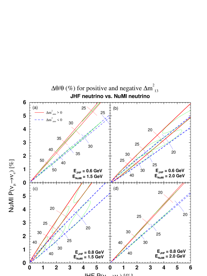
FIG. 1.: Allowed range of $P(\nu_{\mu}\rightarrow\nu_{e})$ for JHF verses $P(\nu_{\mu}\rightarrow\nu_{e})$ for NuMI, which are referred to as “pencils” in the text, are delimited by thick solid (dashed) lines for positive (negative) $\Delta m^{2}_{13}$ for the energies ($E_{JHF}$/GeV, $E_{NuMI}$/GeV) = (a) (0.6,1.5), (oscillation maximum for both experiments) (b) (0.6,2.0), (c) (0.8,1.5) and (d) (0.8,2.0). In the same plot, the positions for some representative values of the fractional variation across the width of the “pencil” of $\theta\equiv\sin\theta_{13}$, $\Delta\theta/\theta$ [%], indicated by numbers, are shown by thin solid arcs. Inside each allowed region, trajectories corresponding to $\sin^{2}2\theta_{13}=0.02$, 0.05 and 0.09 are plotted by dotted lines. The mixing parameters are fixed to be $|\Delta m^{2}_{13}|=2.5\times 10^{-3}$ eV², $\sin^{2}2\theta_{23}=1.0$, $\Delta m^{2}_{12}=+7\times 10^{-5}$ eV² and $\sin^{2}2\theta_{12}=0.85$ whereas $\theta_{13}$ and $\delta$ are assumed to be unknown. The electron density is fixed to be $Y_{e}\rho=1.15$ and 1.4g cm^-3 for JHF and NuMI experiment, respectively. For JHF and NuMI both anti-neutrinos, the roles of $\Delta m^{2}_{13}>~{}0~{}{\rm and}~{}\Delta m^{2}_{13}<~{}0$ are interchanged.

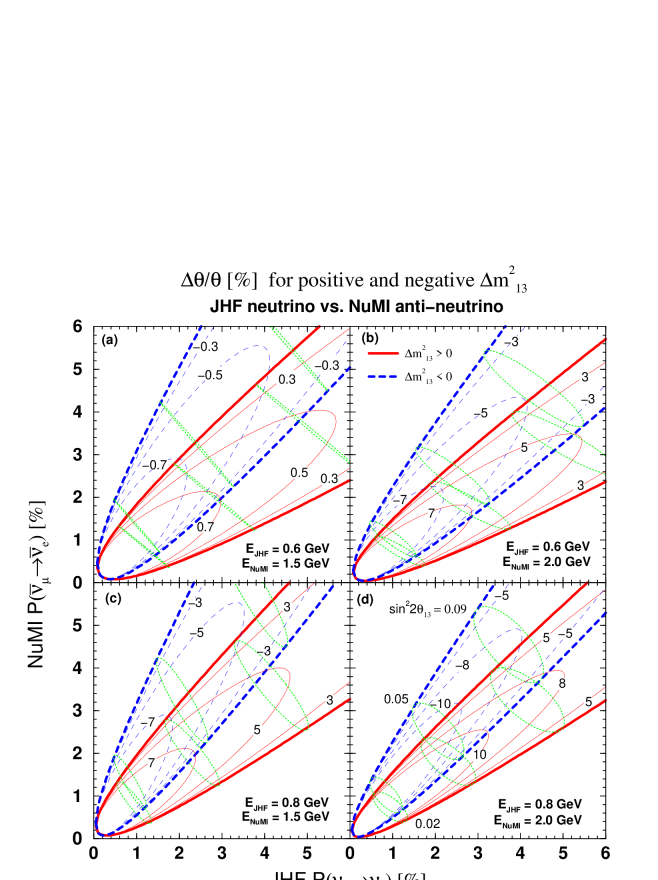
FIG. 2.: Iso-contours of $\Delta\theta/\theta$ [%] are indicated in the allowed range of $P(\nu_{\mu}\rightarrow\nu_{e})$ for JHF verses $P(\bar{\nu}_{\mu}\rightarrow\bar{\nu}_{e})$ for NuMI delimited by solid (dashed) lines for positive (negative) $\Delta m^{2}$ for the same combinations of energies as in Fig. 1. Inside each allowed region, trajectories corresponding to $\sin^{2}2\theta_{13}=0.02$, 0.05 and 0.09 are plotted by dotted lines. The assumption about the mixing parameters are the same as in Fig. 1. For JHF anti-neutrinos and NuMI neutrinos, the roles of $\Delta m^{2}_{13}>~{}0~{}{\rm and}~{}\Delta m^{2}_{13}<~{}0$ are interchanged.

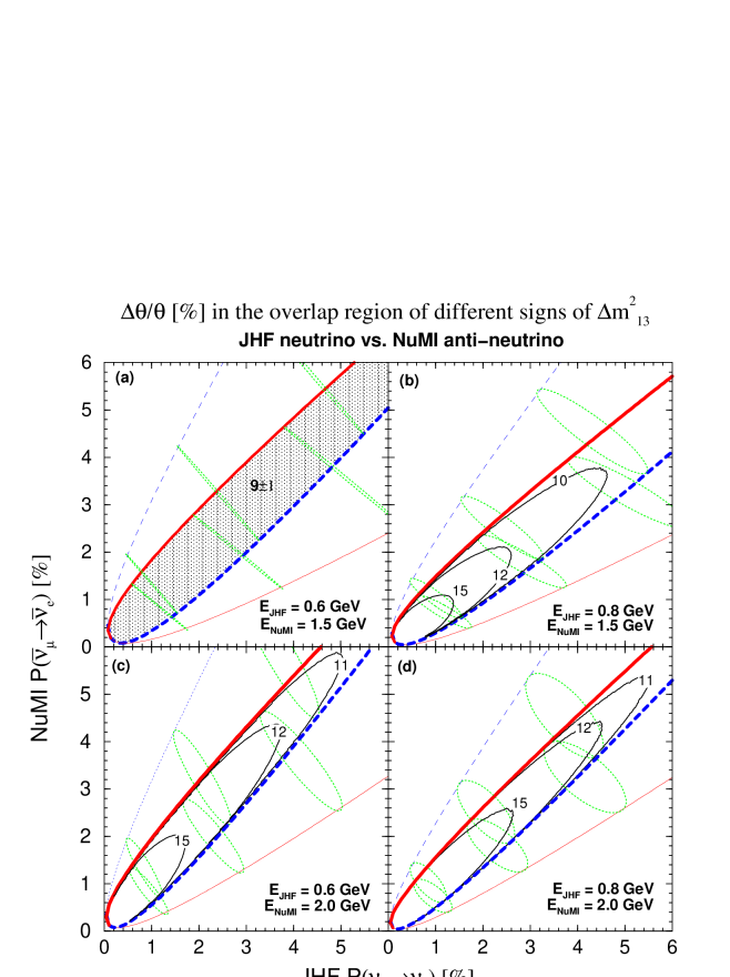
FIG. 3.: Iso-contours of $\Delta\theta/\theta$ [%], except for (a), are indicated in the overlap regions of the allowed range of $P(\nu_{\mu}\rightarrow\nu_{e})$ for JHF verses $P(\bar{\nu}_{\mu}\rightarrow\bar{\nu}_{e})$ for NuMI for the positive and negative signs of $\Delta m^{2}_{13}$ for the combinations of energies shown in Fig. 2. For (a), inside the shaded region, $\Delta\theta/\theta$ varies very little, taking values close to 9 %.

REFERENCES

- [1] K. Eguchi et al. [KamLAND Collaboration], hep-ex/0212021.
- [2] Q. R. Ahmad et al. [SNO collaboration], Phys. Rev. Lett. 87, 071301 (2001); 89, 011301 (2002); 89, 011302 (2002).
- [3] S. Fukuda et al. (Super-Kamiokande Collaboration), Phys. Rev. Lett. 86, 5651 (2001); 86, 5656 (2001); Phys. Lett. B539, 179 (2002).
- [4] L. Wolfenstein, Phys. Rev. D 17, 2369 (1978); S. P. Mikheyev and A. Yu. Smirnov, Yad. Fiz. 42, 1441 (1985) [ Sov. J. Nucl. Phys. 42, 913 (1985)], Nuovo Cim. C9, 17 (1986); S. P. Mikheyev and A. Yu. Smirnov, ZHETF, 91, (1986), [Sov. Phys. JETP, 64, 4 (1986)].
- [5] For the first discussions of the complete MSW triangle including the LMA region, see S. J. Parke, Phys. Rev. Lett. 57, 1275 (1986); S. J. Parke and T. P. Walker, Phys. Rev. Lett. 57, 2322 (1986); J. Bouchez et al, Z. Phys. C 32 (1986) 499; M. Cribier et al., Phys. Lett. B182, 89 (1986); S. P. Mikheyev and A. Yu. Smirnov, Proc. of the 12th Int. Conf Neutrino’86 (Sendai, Japan) eds. T. Kitagaki and H. Yuta, 177 (1986) and Proc. of the Int. Symp. on Weak and Electromagnetic Interactions in Nuclei, WEIN-86, (Heidelberg, 1986), 710.
-
[6]
Kamiokande Collaboration, Y. Fukuda et al.,
Phys. Lett. B335 (1994) 237;
Super-Kamiokande Collaboration, Y. Fukuda et al., Phys. Rev. Lett. 81 (1998) 1562; ibid. 85 (2000) 3999. -
[7]
K2K Collaboration, S. H. Ahn et al.,
Phys. Lett. B 511 (2001) 178;
K2K Collaboration, S. H. Ahn et al., hep-ex/0212007. - [8] Z. Maki, M. Nakagawa and S. Sakata, Prog. Theor. Phys. 28 (1962) 870. We use the standard PDG notation for the MNS matrix, see, Particle Data Group, K. Hagiwara et al., Phys. Rev. D66 (2002) 010001.
- [9] H. Minakata and H. Nunokawa, Phys. Lett. B 504, 301 (2001) [hep-ph/0010240].
- [10] M. T. Keil, G. G. Raffelt, and H. T. Janka, astro-ph/0208035.
- [11] The MINOS Collaboration, P. Adamson et al., MINOS Detectors Technical Design Report, Version 1.0, NuMI-L-337, October 1998
- [12] M. Komatsu, P. Migliozzi, and F. Terranova, hep-ph/0210043.
- [13] Y. Itow et al., hep-ex/0106019.
- [14] D. Ayres et al. hep-ex/0210005.
- [15] J. J. Gomez-Cadenas et al. [CERN working group on Super Beams Collaboration] hep-ph/0105297.
- [16] Y. Kozlov, L. Mikaelyan and V. Sinev, hep-ph/0109277.
- [17] H. Minakata, O. Yasuda, H. Sugiyama, K. Inoue, and F. Suekane, hep-ph/0211111.
- [18] The problem of parameter degeneracy was first uncovered by Fogli and Lisi who noticed that a set of measurements in two different channels and entails two degenerate solutions of (, ); G. Fogli and E. Lisi, Phys. Rev. D54, 3667 (1996).
- [19] J. Burguet-Castell, M. B. Gavela, J. J. Gomez-Cadenas, P. Hernandez and O. Mena, Nucl. Phys. B 608, 301 (2001).
- [20] H. Minakata and H. Nunokawa, JHEP 0110, 001 (2001) [hep-ph/0108085]; Nucl. Phys. Proc. Suppl. 110, 404 (2002) [hep-ph/0111131].
- [21] T. Kajita, H. Minakata, and H. Nunokawa, Phys. Lett. B528 (2002) 245.
- [22] V. Barger, D. Marfatia and K. Whisnant, Phys. Rev. D 65, 073023 (2002).
- [23] H. Minakata, H. Nunokawa, and S. J. Parke, Phys. Rev. D 66, 093012 (2002) [hep-ph/0208163].
- [24] V. Barger, D. Marfatia, and K. Whisnant, Phys. Rev. D 66, 053007 (2002).
- [25] J. Burguet-Castell, M.B. Gavela, J.J. Gomez-Cadenas, P. Hernandez and O. Mena, Nucl. Phys. B 646, 301 (2002).
- [26] A. Donini, D. Meloni, and P. Migliozzi, Nucl. Phys. B 646, 321 (2002).
- [27] V. Barger, D. Marfatia, and K. Whisnant, hep-ph/0210428.
- [28] P. Huber, M. Lindner, and W. Winter, hep-ph/0211300.
- [29] H. Minakata, H. Nunokawa, and S. J. Parke, Phys. Lett B, B537 (2002) 249 [hep-ph/0204171].
- [30] A. Cervera, A. Donini, M. B. Gavela, J. J. Gomez Cadenas, P. Hernandez, O. Mena and S. Rigolin, Nucl. Phys. B579 (2000) 17 [Erratum-ibid. B593 (2000) 731].
- [31] C. Albright et al., arXiv:hep-ex/0008064. M. Apollonio et al., hep-ph/0210192.
- [32] P. Zucchelli, Phys. Lett. B 532, 166 (2002).