Supersymmetric Effects in Deep Inelastic Neutrino-Nucleus Scattering

Abstract

We compute the supersymmetric (SUSY) contributions to $\nu$ (${\bar{\nu}}$)-nucleus deep inelastic scattering in the Minimal Supersymmetric Standard Model (MSSM). We consider the ratio of neutral current to charged current cross sections, ${R_{\nu}}$ and ${R_{\bar{\nu}}}$, and compare with the deviations of these quantities from the Standard Model predictions implied by the recent NuTeV measurement. After performing a model-independent analysis, we find that SUSY loop corrections generally have the opposite sign from the NuTeV anomaly. We discuss one scenario in which a right-sign effect arises, and show that it is ruled out by other precision data. We also study for R parity-violating (RPV) contributions. Although RPV effects could, in principle, reproduce the NuTeV anomaly, such a possibility is also ruled out by other precision electroweak measurements.

I Introduction

Neutrino scattering experiments have played a key role in elucidating the structure of the Standard Model (SM). Recently, the NuTeV collaboration has performed a precise determination of the ratio ${R_{\nu}}$ (${R_{\bar{\nu}}}$) of neutral current (NC) and charged current (CC) deep-inelastic $\nu_{\mu}$ ($\bar{\nu}_{\mu}$)-nucleus cross sectionsnutev02 , which can be expressed as:

$$R_{\nu({\bar{\nu}})}=(g_{L}^{\rm eff})^{2}+r^{(-1)}(g_{R}^{\rm eff})^{2}\ \ \ ,$$ (1)

where $r=\sigma^{CC}_{{\bar{\nu}}N}/\sigma^{CC}_{\nu N}$ and $(g_{L,R}^{\rm eff})^{2}$ are effective hadronic couplings (defined below). Comparing the SM predictionspdg ; erler for $(g_{L,R}^{\rm eff})^{2}$ with the values obtained by the NuTeV Collaboration yields deviations $\delta R_{\nu({\bar{\nu}})}=R_{\nu({\bar{\nu}})}^{\rm exp}-R_{\nu({\bar{\nu}})}^{\rm SM}$

$$\delta R_{\nu}=-0.0033\pm 0.0007,\ \ \ \delta R_{\bar{\nu}}=-0.0019\pm 0.0016.$$ (2)

Within the SM, these results may be interpreted as a test of the scale-dependence of the ${\sin^{2}\theta_{\scriptscriptstyle W}}$ since the $(g_{L,R}^{\rm eff})^{2}$ depend on the weak mixing angle. While the SM prediction for ${\sin^{2}\theta_{\scriptscriptstyle W}}$ at $\mu={M_{\scriptscriptstyle Z}}$ has been confirmed with high precision at LEP and SLC, the predicted running of this parameter to lower scales has yet to be studied systematically. The results from the NuTeV measurement imply a $+3\sigma$ deviation at $\mu\sim 10$ GeV, while the current value of the cesium weak charge, extracted from atomic parity-violation (PV), implies agreement with the predicted SM running at a much lower scaleapv . Measurements of the PV asymmetries in polarized $ee$ and $ep$ scattering will provide further tests of this running at $\mu\sim 0.2$ GeV slac ; qweak .

This interpretation of the NuTeV results has been the subject of some debate. Unaccounted for QCD effects, such as charge symmetry-breaking in parton distributions or nuclear shadowingmiller , have been proposed as possible remedies for the anomaly. Alternatively, one may consider physics beyond the SM, as reviewed in Ref. davidson . In what follows, we focus on one new physics scenario, namely, supersymmetry (SUSY). While a brief discussion of SUSY is given in Ref. davidson , an extensive, detailed treatment has yet to appear in the literature. Because SUSY is one of the most strongly-motivated extensions of the SM, undertaking such an analysis is a timely endeavor. The goal of the present study is to provide this comprehensive treatment.

In performing our analysis, we work within the framework of the Minimal Supersymmetric Standard Model (MSSM), which remains the standard baseline for considering SUSY effects in precision observables. Typically, MSSM studies adopt one or more models of SUSY-breaking mediation, thereby vastly simplifying the task of analyzing the MSSM parameter space. Here, however, we carry out a model-independent treatment, avoiding the choice of a specific mechanism for SUSY-breaking mediation. Since generic features of the superpartner spectrum implied by the most widely adopted SUSY-breaking models may not be consistent with precision data kurylov02 , we wish to determine whether there exist any choices for MSSM parameters that could account for the NuTeV result, even if such choices lie outside the purview of standard SUSY-breaking models.

We find that it is difficult – if not impossible – to choose MSSM parameters so as to improve agreement with the NuTeV result. When R parity is conserved and SUSY effects only arise via radiative corrections, the magnitude of their contribution is generally too small for the NuTeV anomaly to generate significant constraints. Moreover, for nearly all parameter choices, the sign of the SUSY corrections to ${R_{\nu}}$ and ${R_{\bar{\nu}}}$ is opposite to that of the NuTeV anomaly. We do find one scenario – not considered in Ref. davidson – under which SUSY loops generate a right sign effect with relatively large magnitude, but this scenario is presently inconsistent with other precision, electroweak data.

We also consider possible tree-level contributions from R parity-violating (RPV) interactions, whose presence would render the lightest supersymmetric particle (LSP) unstable. We observe that purely leptonic RPV effects, which arise via the definition of ${\sin^{2}\theta_{\scriptscriptstyle W}}$, could in principle also generate a right sign effect to account for the NuTeV anomaly. However, precision data also limits the magnitude of this contribution to be considerably smaller than necessary. On the other hand, the NuTeV result does yield new constraints on possible semileptonic RPV interactions.

In short, our qualitative conclusions agree with those of Ref. davidson , though we believe we have carried out a more exhaustive analysis. Thus, one would have to look to more exotic new physics possibilities, such as a $Z^{\prime}$ boson coupling only to second generation fermions, if SM QCD effects are ultimately unable to explain the NuTeV anomaly. We note that the situation here contrasts with that for the PV electron scattering asymmetries, where the SM contribution is fortuitously suppressed and where SUSY radiative corrections could, in principle, produce observable contributionskurylov02b .

The analysis leading to these conclusions is organized in the remainder of the paper as follows. In Section II, we discuss general features of MSSM contributions to $\nu_{\mu}$ ($\bar{\nu}_{\mu}$)-nucleus scattering, including both SUSY loop corrections and RPV effects. Section III gives details of the loop computation as well as the scan over the MSSM parameter space. In Section IV, we give the RPV analysis, including results of a fit to other precision data. Section V contains a summary of our results. Explicit formulae for loop corrections with relevant Feynman rules are given in the Appendices.

II $\nu_{\mu}N$ (${\bar{\nu}_{\mu}}N$) Scattering in the MSSM: General Considerations

For momentum transfers $q^{\mu}$ satisfying $|q^{2}|<<{M^{2}_{\scriptscriptstyle Z}}$, the neutrino-quark interactions can be represented with sufficient accuracy by an effective four fermion Lagrangian:

$${\cal L}_{\nu q}^{NC} = -{G_{\mu}\rho^{NC}_{\nu N}\over\sqrt{2}}{\bar{\nu}}_{\mu}\gamma^{\lambda}(1-\gamma_{5})\nu_{\mu}\sum_{q}{\bar{q}}\gamma_{\lambda}[2\epsilon_{L}^{q}P_{L}+2\epsilon_{R}^{q}P_{R}]q$$ (3)

$${\cal L}_{\nu q}^{CC} = -{G_{\mu}\rho^{CC}_{\nu N}\over\sqrt{2}}{\bar{\mu}}\gamma^{\lambda}(1-\gamma_{5})\nu_{\mu}{\bar{u}}\gamma_{\lambda}(1-\gamma_{5})d+{\rm h.c.}\ \ \ ,$$ (4)

where $P_{L}=(1-\gamma_{5})/2$, $P_{R}=(1+\gamma_{5})/2$ and

$$\epsilon_{L}^{q} = I_{L}^{3}-Q_{q}\kappa_{\nu}{\sin^{2}\theta_{\scriptscriptstyle W}}+\lambda_{L}^{q}$$ (5)

$$\epsilon_{R}^{q} = -Q_{q}\kappa_{\nu}{\sin^{2}\theta_{\scriptscriptstyle W}}+\lambda_{R}^{q}\ \ \ .$$ (6)

The parameters $\rho_{\nu N}^{NC}=\rho_{\nu N}^{CC}=\kappa_{\nu}=1$ and $\lambda_{L,R}^{q}=0$ at tree-level in the SM. These quantities differ from their tree-level values when ${\cal O}(\alpha)$ corrections in the SM or MSSM are included or when other new physics contributions arise. The precise values of these quantities individually are renormalization scheme-dependent. When computing MSSM loop contributions, we use the modified dimensional reduction (${\overline{DR}}$) scheme, in which the spatial dimension of momenta are continued into $d=4-2\epsilon$ dimensions while the Dirac matrices remain four dimensional, as required by SUSY invariance. Quantities renormalized in the ${\overline{DR}}$ scheme will be indicated by a hat. Note also that for the neutrino reactions of interest here, $\rho_{\nu N}^{NC}$, $\rho_{\nu N}^{CC}$, and $\kappa_{\nu}$ are universal (independent of quark flavor), while the $\lambda_{L,R}^{q}$ are flavor-dependent.

The NC to CC cross section ratios ${R_{\nu}}$ and ${R_{\bar{\nu}}}$ can be expressed in terms of the above parameters via the effective couplings $(g_{L,R}^{\rm eff})^{2}$ appearing in Eq. (1) in a straightforward way:

$$(g_{L,R}^{\rm eff})^{2}=\left({{\hat{M}}_{Z}^{2}\over{\hat{M}}_{W}^{2}}\right)^{2}\left({{\hat{M}}_{W}^{2}-q^{2}\over{\hat{M}}_{Z}^{2}-q^{2}}\right)^{2}\left({\rho_{\nu N}^{NC}\over\rho_{\nu N}^{CC}}\right)^{2}\sum_{q}\ (\epsilon_{L,R}^{q})^{2}\ \ \ .$$ (7)

The SM values for these quantities arepdg ; erler $(g_{L}^{\rm eff})^{2}=0.3042$ and $(g_{R}^{\rm eff})^{2}=0.0301$ while the NuTeV results imply $(g_{L}^{\rm eff})^{2}=0.3005\pm 0.0014$ and $(g_{R}^{\rm eff})^{2}=0.0310\pm 0.0011$.

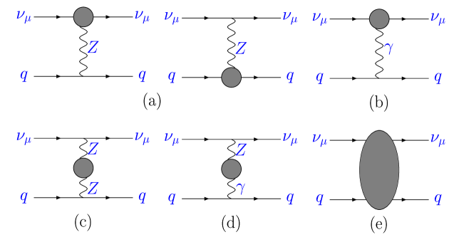
Figure 1: One loop contributions to the neutrino-quark neutral current amplitude. The blob denotes the one loop irreducible diagram or the counter term. The Feynman diagrams for the external leg corrections are not shown explicitly.

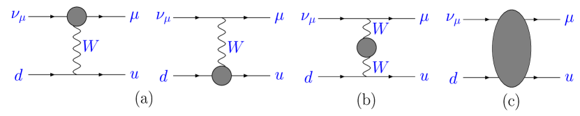
Figure 2: One loop contributions to the neutrino-quark charge current amplitude. The blob denotes the one loop irreducible diagram or the counter term. The Feynman diagrams for the external leg corrections are not shown explicitly.

In what follows, we concentrate on the MSSM contributions to $\rho^{NC,CC}_{\nu N}$, $\kappa_{\nu}$, $\lambda_{L,R}^{q}$, ${R_{\nu}}$, and ${R_{\bar{\nu}}}$. When the R-parity quantum number $(-1)^{3(B-L)+2s}$ is conserved, the MSSM contributes to these quantities only via loop effects. The relevant diagrams are shown in Figs. 1-2 and the Appendices. Note that all gauge boson self energy corrections, as well as leptonic vertex and external leg corrections, contribute only to the universal parameters $\rho_{\nu N}^{NC,CC}$ and $\kappa_{\nu}$. For the NC amplitudes, non-universal box diagrams and quark vertex and external leg corrections (${\hat{\delta}}_{VB}^{L,R;q}$) are contained in the $\lambda_{L,R}^{q}$. All CC box graphs as well as hadronic vertex and external leg contributions (${\hat{\delta}}_{VB}^{CC}$) appear in $\rho_{\nu N}^{CC}$. The CC box graphs also generate amplitudes involving products of scalar and pseudoscalar currents. However, the corresponding ${\cal O}(\alpha)$ corrections to ${R_{\nu}}$ and ${R_{\bar{\nu}}}$ are suppressed by lepton and quark masses, so we neglect them here. In terms of these various corrections, the renormalized parameters are

$$\rho_{\nu N}^{CC} = 1+{{\hat{\Pi}}_{WW}(q^{2})\over{M^{2}_{\scriptscriptstyle W}}-q^{2}}-{{\hat{\Pi}}_{WW}(0)\over{M^{2}_{\scriptscriptstyle W}}}+{\hat{\delta}}_{VB}^{CC}-{\hat{\delta}}_{VB}^{\mu}$$ (8)

$$\rho_{\nu N}^{NC} = 1+{{\hat{\Pi}}_{ZZ}(q^{2})\over{M^{2}_{\scriptscriptstyle Z}}-q^{2}}-{{\hat{\Pi}}_{WW}(0)\over{M^{2}_{\scriptscriptstyle W}}}+{\hat{\delta}}_{V}^{\nu}-{\hat{\delta}}_{VB}^{\mu}$$ (9)

$$\kappa_{\nu} = {{\hat{c}}\over{\hat{s}}}{{\hat{\Pi}}_{Z\gamma}(q^{2})\over q^{2}}+{\delta\sin^{2}\hat{\theta}_{W}\over\sin^{2}\hat{\theta}_{W}}-4{\hat{c}}^{2}{\hat{F}}_{A,\nu}(q^{2})$$ (10)

$$\lambda_{L,R}^{q} = {\hat{\delta}}_{VB}^{L,R;q}\ \ \ ,$$ (11)

where ${\hat{\Pi}}_{VV^{\prime}}(q^{2})$ are the gauge boson self-energies renormalized in the ${\overline{DR}}$ scheme at a scale $\mu={M_{\scriptscriptstyle Z}}$; ${\hat{\delta}}_{VB}^{\mu}$ denote vertex, external leg, and box graph corrections entering the muon-decay amplitude; and ${\hat{\delta}}_{V}^{\nu}$ indicates the neutral current neutrino vertex and lepton external leg correction. Note that the muon decay corrections enter the semileptonic amplitudes since the Fermi constant $G_{\mu}$ is taken from the muon lifetime. The correction ${\hat{F}}_{A,\nu}$ arises from the $\nu_{\mu}$ charge radius. Superpartner loop contributions to ${\hat{\Pi}}_{Z\gamma}(q^{2}=0)$ are zero, so that the corresponding contributions to $\kappa_{\nu}$ are finite at the photon point. The shift in $\sin^{2}\hat{\theta}_{W}$ arises from its definition in terms of $\alpha$, $G_{\mu}$, and ${M_{\scriptscriptstyle Z}}$

$${\hat{s}}^{2}{\hat{c}}^{2}={\pi\alpha\over\sqrt{2}M_{Z}^{2}G_{\mu}[1-\Delta{\hat{r}}(M_{Z})]}$$ (12)

${\hat{s}}^{2}=1-{\hat{c}}^{2}=\sin^{2}\hat{\theta}_{W}(M_{Z})$ andpierce

$$\Delta{\hat{r}}={{\hat{\Pi}}^{\prime}}_{\gamma\gamma}(0)+2{{\hat{s}}\over{\hat{c}}}{{\hat{\Pi}}_{Z\gamma}(0)\over M_{Z}^{2}}-{{\hat{\Pi}}_{ZZ}(M_{Z}^{2})\over M_{Z}^{2}}+{{\hat{\Pi}}_{WW}(0)\over M_{W}^{2}}+{\hat{\delta}}_{VB}^{\mu}$$ (13)

with ${{\hat{\Pi}}^{\prime}}_{\gamma\gamma}(q^{2})={\hat{\Pi}}_{\gamma\gamma}(q^{2})/q^{2}$. Writing $\Delta{\hat{r}}=\Delta{\hat{r}}^{\rm SM}+\Delta{\hat{r}}^{\rm SUSY}$ one has

$${\delta{\hat{s}}^{2}_{\rm SUSY}\over{\hat{s}}^{2}}={{\hat{c}}^{2}\over{\hat{c}}^{2}-{\hat{s}}^{2}}\Delta{\hat{r}}^{\rm SUSY}\ \ \ .$$ (14)

In Section III, we discuss our computation of the MSSM loop contributions to these parameters in detail; explicit expression for the various loop amplitudes appears in the Appendices.

When $R$-parity is not conserved, however, new tree-level contributions appear. The latter are generated by the $B-L$ violating superpotential

$$W_{\scriptscriptstyle RPV}=\frac{1}{2}\lambda_{ijk}L_{i}L_{j}{\bar{E}}_{k}+\lambda^{\prime}_{ijk}L_{i}Q_{j}{\bar{D}}_{k}+\frac{1}{2}\lambda^{\prime\prime}_{ijk}{\bar{U}}_{i}{\bar{D}}_{j}{\bar{D}}_{k}\ \ \ ,$$ (15)

where $L_{i}$ and $Q_{i}$ denote lepton and quark SU(2)_L doublet superfields, $E_{i}$, $U_{i}$, and $D_{i}$ are singlet superfields and the $\lambda_{ijk}$ etc. are a priori unknown couplings. We have neglected additional lepton-Higgs mixing term in Eq. (15) for simplicity. In order to avoid unacceptably large contributions to the proton decay rate, we set the $\Delta B\not=0$ couplings $\lambda^{\prime\prime}_{ijk}$ to zero. The purely leptonic terms ($\lambda_{12k}$) contribute to neutrino scattering amplitudes via the normalization of CC and NC amplitudes to $G_{\mu}$ and through the definition of $\sin^{2}\hat{\theta}_{W}$mrm00 . The remaining semileptonic, $\Delta L=\pm 1$ interactions ($\lambda^{\prime}_{ijk}$) give direct contributions to the neutrino scattering amplitudes. The latter may be obtained computing the Feynman amplitudes in Fig. 3 and performing a Fierz reordering. For neutrino-quark scattering, one obtains the effective Lagrangian

$${\cal L}_{\scriptscriptstyle RPV}^{\scriptscriptstyle EFF} = -{|\lambda^{\prime}_{2k1}|^{2}\over 2M^{2}_{\tilde{d}^{k}_{L}}}{\bar{d}}_{R}\gamma^{\mu}d_{R}{\bar{\nu}}_{\mu L}\gamma_{\mu}\nu_{\mu L}+{|\lambda^{\prime}_{21k}|^{2}\over 2M^{2}_{\tilde{d}^{k}_{R}}}{\bar{d}}_{L}\gamma^{\mu}d_{L}{\bar{\nu}}_{\mu L}\gamma_{\mu}\nu_{\mu L}$$ (16)

$$-{|\lambda^{\prime}_{21k}|^{2}\over 2M^{2}_{\tilde{d}^{k}_{R}}}\Biggl{[}{\bar{u}}_{L}\gamma^{\mu}d_{L}{\bar{\mu}}_{L}\gamma_{\mu}\nu_{\mu L}+{\rm h.c.}\Biggr{]}\ \ \ ,$$

where we have taken $|q^{2}|<<M_{\tilde{f}}^{2}$ and have retained only the semileptonic terms relevant to $\nu_{\mu}$-$q$ scattering.

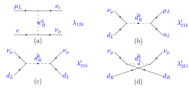
Figure 3: Tree level RPV contributions to muon decay [plot (a)], $\nu_{\mu}-q$ charged current [plot (b)] and $\nu_{\mu}-q$ neutral current [plots (c) and (d)] amplitudes.

In terms of these parameters, the shifts induced in the effective $\nu_{\mu}$ (${\bar{\nu}_{\mu}}$)-$N$ parameters $\rho_{\nu N}^{CC,\ NC}$ and $\epsilon^{q}_{L,R}$ are

$$\delta\rho_{\nu N}^{NC} = \Delta_{12k}({\tilde{e}}^{k}_{R})$$ (17)

$$\delta\rho_{\nu N}^{CC} = \delta\rho_{\nu N}^{NC}+\Delta^{\prime}_{21k}({\tilde{d}}^{k}_{R})$$ (18)

$$\delta\epsilon_{L}^{d} = -\Delta^{\prime}_{21k}({\tilde{d}}^{k}_{R})+\frac{1}{3}{\lambda_{x}}\Delta_{12k}({\tilde{e}}^{k}_{R})$$ (19)

$$\delta\epsilon_{R}^{d} = -\Delta^{\prime}_{2k1}({\tilde{d}}^{k}_{L})+\frac{1}{3}{\lambda_{x}}\Delta_{12k}({\tilde{e}}^{k}_{R})$$ (20)

$$\delta\epsilon^{u}_{L}=\delta\epsilon^{u}_{R} = -\frac{2}{3}{\lambda_{x}}\Delta_{12k}({\tilde{e}}^{k}_{R})\ \ \ ,$$ (21)

where

$$\Delta_{ijk}({\tilde{f}})={|\lambda_{ijk}|^{2}\over 4\sqrt{2}G_{\mu}M^{2}_{\tilde{f}}}$$ (22)

andmrm00

$${\lambda_{x}}\approx{{\hat{s}}^{2}{\hat{c}}^{2}\over{\hat{c}}^{2}-{\hat{s}}^{2}}\approx 0.35\ \ \ .$$ (23)

The corresponding shifts in $R_{\nu(\bar{\nu})}$ are

$$\delta R_{\nu(\bar{\nu})} = \lambda_{x}[-\frac{4}{3}\epsilon_{L}^{u}+\frac{2}{3}\epsilon_{L}^{d}][1+r^{(-1)}]\Delta_{12k}(\tilde{e}_{R}^{k})-2[R_{\nu(\bar{\nu})}^{\rm SM}+\epsilon_{L}^{d}]\Delta_{21k}^{\prime}(\tilde{d}_{R}^{k})$$

$$\ \ \ +2r^{(-1)}\epsilon_{R}^{d}\Delta_{2k1}^{\prime}(\tilde{d}_{L}^{k})$$

$$\approx -0.25[1+r^{(-1)}]\Delta_{12k}(\tilde{e}_{R}^{k})-2[R_{\nu(\bar{\nu})}^{\rm SM}-0.43]\Delta_{21k}^{\prime}(\tilde{d}_{R}^{k})+1.6r^{(-1)}\Delta_{2k1}^{\prime}(\tilde{d}_{L}^{k})\ \ \ .$$

As we discuss in Section IV, $\Delta_{12k}({\tilde{e}}^{k}_{R})$ and $\Delta^{\prime}_{21k}({\tilde{d}}^{k}_{R})$ are constrained by other precision electroweak data, while $\Delta^{\prime}_{2k1}({\tilde{d}}^{k}_{L})$ is relatively unconstrained. In Eq. (II), the coefficients of $\Delta^{\prime}_{21k}({\tilde{d}}^{k}_{R})$ and $\Delta^{\prime}_{2k1}({\tilde{d}}^{k}_{L})$ are positive, while the coefficient of $\Delta_{12k}({\tilde{e}}^{k}_{R})$ is negative. Since the $\Delta_{ijk}$ are non-negative, we would require sizable value of $\Delta_{12k}({\tilde{e}}^{k}_{R})$ and rather small values of $\Delta^{\prime}_{21k}({\tilde{d}}^{k}_{R})$ and $\Delta^{\prime}_{2k1}({\tilde{d}}^{k}_{L})$ to account for the negative shifts in ${R_{\nu}}$ and ${R_{\bar{\nu}}}$ implied by the NuTeV analysis. The present constraints on $\Delta_{12k}({\tilde{e}}^{k}_{R})$, however, are fairly stringent, ruling out sizable values for the semileptonic corrections with fairly high confidence.

III SUSY Loop Contributions

Instead of working in a specific SUSY breaking scenario, we perform a model-independent analysis by varying all the possible soft SUSY-breaking parametershaber . Although such an approach is insensitive to the effects of any particular SUSY breaking parameter, it does allow us to obtain the size of SUSY contributions in the most general way. In our analysis, we set the momentum transfer $q^{2}=0$.

We first compute loop effects only (R-parity being conserved) by scanning over the MSSM parameters in the ranges shown in Table. 1. Here, $\tan\beta=v_{u}/v_{d}$ is the ratio of the up and down type Higgs vacuum expectation values; $\mu$ is bilinear Higgs coupling in the supersymmetric Lagrangian, which gives the mass to the Higgsino; $M_{1}$, $M_{2}$ and $M_{\tilde{g}}$ are the masses for ${\rm U}(1)_{Y}$, ${\rm SU}(2)_{L}$ and ${\rm SU}(3)_{c}$ gaugino, respectively; $M^{i}_{\tilde{f}_{L,R}}$ are the diagonal mass parameters for the left- and right- handed squarks and sleptons of generation $i$, while $M^{i}_{\tilde{f}_{LR}}$ are the left-right mixing parameters. In order to avoid unacceptably large flavor-changing neutral currents, we do not allow for flavor mixing between squark generations but do allow for superpartners of different generations to have different masses.

Parameter	Min	Max
$\tan\beta$	1.4	60
${\tilde{M}}$	50 GeV	1000 GeV
$M^{i}_{\tilde{f}_{LR}}$	-1000 GeV	1000 GeV

Table 1: Ranges of SUSY parameters scanned. Here, ${\tilde{M}}$ denotes any of $|\mu|$, $M_{1,2,{\tilde{g}}}$, or the diagonal sfermion mass parameters $M^{i}_{{\tilde{f}}_{L,R}}$. The $\mu$ parameter can take either sign. The generation index $i$ runs from 1 to 3.

In randomly choosing values for these parameters, we follow the conventional practice of using a linear distribution for all parameters except $\tan\beta$, for which we use a logarithmic distribution. We discard any points that yield SUSY particle masses below present collider lower bounds. In addition, we impose constraints from the $Z$-pole electroweak precision measurements, which are embodied in terms of the three oblique parameters $S$, $T$ and $U$ peskin . To that end, we express the SUSY shifts in $\rho_{\nu N}^{NC}$ and $\kappa_{\nu}$ in terms of these quantities:

$$\delta\rho^{NC}_{\nu N} = {\hat{\alpha}}T-{\hat{\delta}}_{VB}^{\mu}$$

$$\delta\kappa_{\nu} = \left({{\hat{c}}^{2}\over{\hat{c}}^{2}-{\hat{s}}^{2}}\right)\left({{\hat{\alpha}}\over 4{\hat{s}}^{2}{\hat{c}}^{2}}S-{\hat{\alpha}}T+{\hat{\delta}}_{VB}^{\mu}\right)$$ (25)

$$+{{\hat{c}}\over{\hat{s}}}\Bigl{[}{{\hat{\Pi}}_{Z\gamma}(q^{2})\over q^{2}}-{{\hat{\Pi}}_{Z\gamma}(M_{Z}^{2})\over M_{Z}^{2}}\Bigr{]}^{\rm SUSY}$$

$$+\Bigl{(}{{\hat{c}}^{2}\over{\hat{c}}^{2}-{\hat{s}}^{2}}\Bigr{)}\Bigl{[}-{{\hat{\Pi}}_{\gamma\gamma}(M_{Z}^{2})\over M_{Z}^{2}}+{\Delta{\hat{\alpha}}\over{\hat{\alpha}}}\Bigr{]}^{\rm SUSY}-4{\hat{c}}^{2}\hat{F}^{\rm SUSY}_{A,\nu}(q^{2})\ \ \ ,$$

where remaining terms proportional to $q^{2}$ are negligible and have been dropped. Here $\Delta{\hat{\alpha}}$ is the SUSY contribution to the difference between the fine structure constant and the electromagnetic coupling renormalized at $\mu=M_{Z}$: $\Delta{\hat{\alpha}}=\left[{\hat{\alpha}}(M_{Z})-\alpha\right]^{\rm SUSY}$.

Note that only $S$ and $T$ enter these expressions. Since these parameters are correlated, we use the 95$\%$ C.L. $S-T$ constraints pdg and retain only those parameter choices consistent with these constraints. We observe that this procedure is not entirely self-consistent, since we have not taken into account non-oblique corrections to $Z$-pole observables in deriving the oblique parameter constraints. Nevertheless, the essential, qualitative implications of precision $Z$-pole data for SUSY loop effects on the $\nu_{\mu}$-$q$ parameters are unaffected by this inconsistency. We also omit parameter choices generating too large a SUSY contribution to the muon anomalous magnetic momentmuon . Doing so limits left-right mixing for second generation sleptons to be fairly small.

Before presenting our results, we also comment on the inputs used in Ref. davidson . In that study, the authors only investigated the slepton contribution with four MSSM parameters: $M_{1}$, $\mu$, $\tan\beta$ and $M_{\tilde{l}}$, assuming the GUT relation for the gaugino masses and the slepton mass degeneracy. In our analysis, we include the contribution from both the squark and slepton sectors, taking into account sfermion left-right mixing, and allowing for non-universality between generations.

With a sample of about 3000 randomly selected parameter sets, we calculated the MSSM contributions to $R_{\nu}$ and $R_{\bar{\nu}}$. The numerical results are shown in Fig. 4(a). We observe that $R_{\nu}$ and $R_{\bar{\nu}}$ are highly correlated. This correlation arises because MSSM contributions to the $r^{(-1)}(g_{R}^{\rm eff})^{2}$ term in Eq. (1) are small, while the contribution to the $(g_{L}^{\rm eff})^{2}$ terms are the same for both $R_{\nu}$ and $R_{\bar{\nu}}$. We also find that the magnitude of $\delta R_{\nu,\bar{\nu}}$ is dominated by the SUSY contributions to $T$ (see Figs. 4(b) and 5), which is sensitive to isospin-breaking in the SUSY spectrum. It is bounded above by other precision electroweak data, thereby limiting the size of possible SUSY loop contributions to ${R_{\nu}}$ and ${R_{\bar{\nu}}}$ to be considerably smaller than the deviations in Eq. (2). A breakdown of the various classes contributions is given in Fig. 5. More significantly, the sign of the SUSY loop corrections is nearly always positive, in contrast to the sign of the NuTeV anomaly.

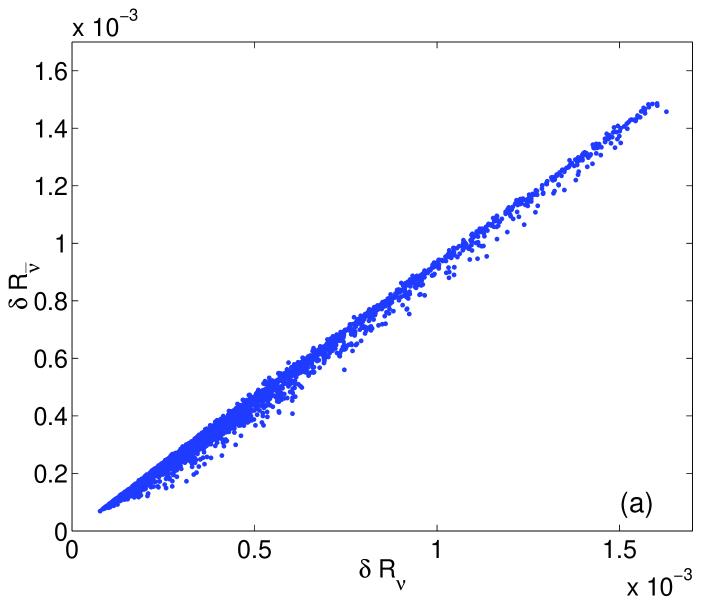
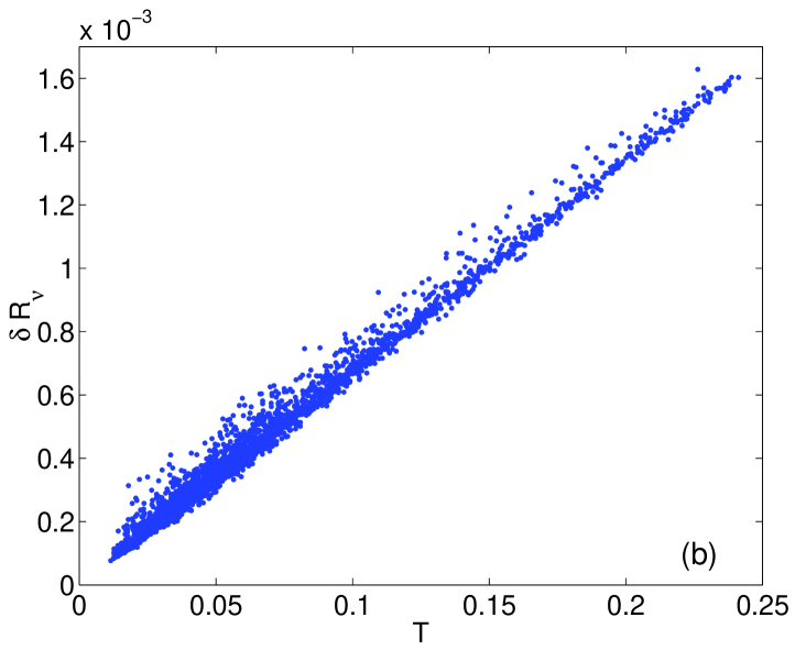
Figure 4: Plot (a) gives the MSSM contribution to $R^{\nu}$ and $R^{\bar{\nu}}$ with MSSM parameters chosen randomly from range shown in Table. 1. Plot (b) shows the dependence of $\delta R_{\nu}$ on the oblique parameter $T$ with the random MSSM parameter set.

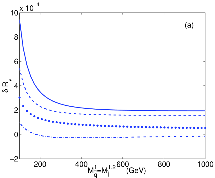
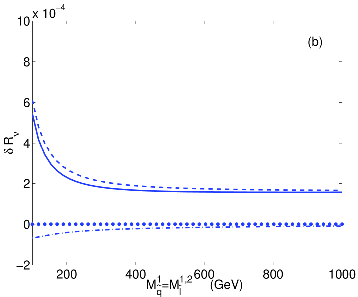
Figure 5: Contributions to $\delta R_{\nu}$ from $\delta\rho^{NC}-\delta\rho^{CC}$ (dashed line), $\delta\kappa$ (dotted line) and $\lambda^{NC}$ (dash-dotted line). The solid line is the sum of all the contributions to $\delta R_{\nu}$. Plot(b) shows the size of various components of $\delta\rho^{NC}-\delta\rho^{CC}$ (solid line): $T$ (dashed line), $\hat{\delta}_{VB}^{\mu}$ (dotted line) and $\hat{\delta}_{VB}^{NC}-\hat{\delta}_{VB}^{CC}$ (dash-dotted line). The $x$-axis is the common first generation squark mass and first and second generation slepton mass. The other MSSM parameters are chosen to be $\tan\beta=10$, $2M_{1}=M_{2}=\mu=200$ GeV. The mass for the second and third generation squarks and third generation slepton are taken to be 1000 GeV.

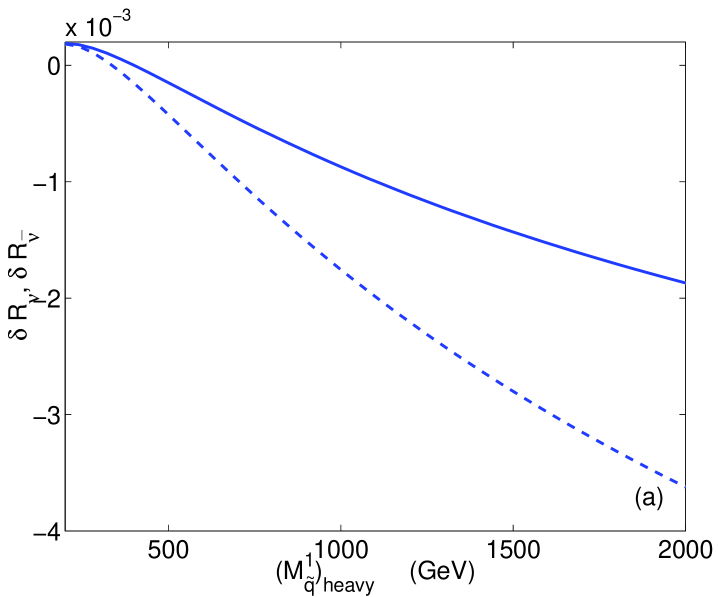
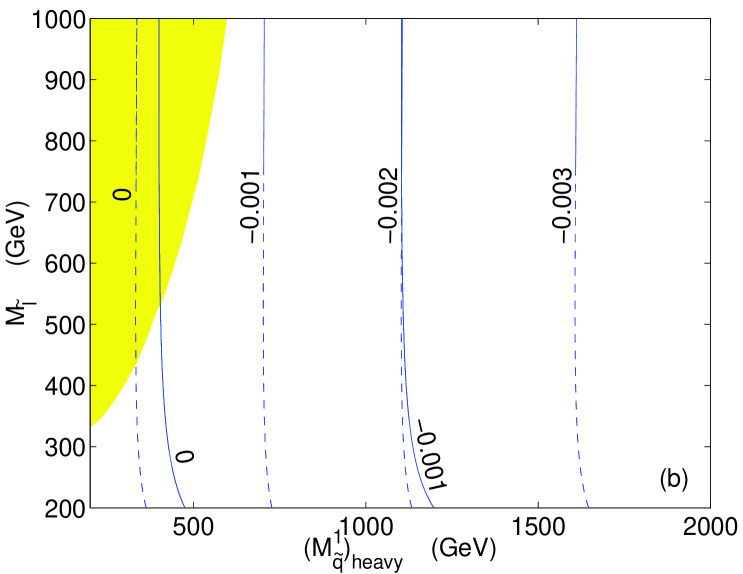
Figure 6: Plot (a) shows the MSSM contribution to $R^{\nu}$ (solid line) and $R^{\bar{\nu}}$ (dashed line) with respect to the heavy first generation squark masses $M_{\tilde{u}}^{1}=M_{\tilde{d}}^{1}\equiv M_{\tilde{q}}^{1}$, when the light first generation squark mass is fixed to be 200 GeV and the left-right mixing angle in fixed to be $\theta_{\tilde{u}}^{1}=\theta_{\tilde{d}}^{1}=\pi/4$. No $L-R$ mixing for other squarks and sleptons is assumed. The rest of the MSSM parameters are chosen to be: $2M_{1}=M_{2}=\mu=200$ GeV, $M_{\tilde{g}}=200$ GeV, $M_{\tilde{l}}=1000$ GeV, $M_{\tilde{q}}^{2,3}=1000$ GeV and $\tan\beta=10$. Plot (b) shows the contours for the shifts $\delta R_{\nu}$ (solid line) and $\delta R_{\bar{\nu}}$ (dashed line) in the plane of slepton mass and heavy first generation squark masses. Slepton mass degeneracy is assumed. The rest of the MSSM parameters are the same as those used in plot (a). The shaded region in (b) shows the region preferred by charge current universality.

We do, however, find one corner of the parameter space which admits a negative loop contribution. This scenario involves gluino loops, whose effect can become large and negative when the first generation up-type squark and down-type squarks are nearly degenerate and left-right mixing is close to maximal. In this particular region of the MSSM parameter space, there is no gluino loop correction to the quark charged and neutral vector currents, while the axial currents receive large corrections. When $M^{2,3}_{{\tilde{f}}_{LR}}=0$ and and the second and third generation soft parameters are sufficiently heavy (corresponding to a small value for $T$), the gluino contribution could give rise to a negative correction to $R_{\nu,\bar{\nu}}$, as shown in Fig. 6 (a). In fact, the gluino contribution could be as much as few$\times 10^{-3}$ in magnitude. As illustrated in Fig. 6(b), however, equal and large left-right mixing for both up- and down-type squarks is inconsistent with the other precision electroweak inputs, such as the $M_{W}$ and charged current universalitykurylov02 . The shaded region in Fig. 6(b) shows the region preferred by these other inputs in the $(M_{\tilde{q}}^{1})_{\rm heavy}$ and $M_{\tilde{\ell}}$ plane. Note that a shift in $|V_{us}|$, as implied by the recent analysis of charged $K_{\ell 3}$ decays in the E865 experiment at Brookhaven National Laboratorysher , would increase the shaded region in Fig. 6.

It is interesting to note that even if other precision data did not rule out this gluino loop effect, it could not account for the apparent deviation of ${\sin^{2}\theta_{\scriptscriptstyle W}}$ from the SM prediction implied by the NuTeV analysis. The latter relies on a modified version of the Paschos-Wolfenstein relationpwrel

$$R^{-}\equiv{{R_{\nu}}-r{R_{\bar{\nu}}}\over 1-r}=\frac{1}{2}(1-2{\sin^{2}\theta_{\scriptscriptstyle W}})+\cdots$$ (26)

where we have shown the SM prediction for $R^{-}$ with the $+\cdots$ indicating higher-order corrections. In practice, the extraction of ${\sin^{2}\theta_{\scriptscriptstyle W}}$ relies on a slightly different combination of ${R_{\nu}}$ and ${R_{\bar{\nu}}}$ in the numerator,

$${\tilde{R}}^{-}\equiv{{R_{\nu}}-\xi{R_{\bar{\nu}}}\over 1-r}$$ (27)

with $\xi$ chosen to be slightly different from $r$ in order to minimize charm quark mass uncertainties in the ${\sin^{2}\theta_{\scriptscriptstyle W}}$ extractionheidi . It is straightforward to show that gluino loop contributions to ${\tilde{R}}^{-}$ are proportional to $\xi-r$, thereby minimizing their impact on ${\sin^{2}\theta_{\scriptscriptstyle W}}$. Specifically, we find that for maximal left-right mixing $\theta_{\tilde{u}}^{1}=\theta_{\tilde{d}}^{1}=\pi/4$,

$${\tilde{R}}^{-} = {\alpha_{s}\over 3\pi}(\xi-r){1+r\over r(1-r)}{\hat{s}}^{2}\left(1-{5\over 9}{\hat{s}}^{2}\right)\Biggl{(}2V_{2}\left[M_{\tilde{g}},(M_{\tilde{q}}^{1})_{\rm heavy},(M_{\tilde{q}}^{1})_{\rm light}\right]$$ (28)

$$- V_{2}\left[M_{\tilde{g}},(M_{\tilde{q}}^{1})_{\rm heavy},(M_{\tilde{q}}^{1})_{\rm heavy}\right]-V_{2}\left[M_{\tilde{g}},(M_{\tilde{q}}^{1})_{\rm light},(M_{\tilde{q}}^{1})_{\rm light}\right]\Biggr{)}$$

where $\alpha_{s}$ is the strong coupling constant and $V_{2}(M,m_{1},m_{2})$ is defined in Eq. (B.3).

In summary, it is difficult to explain the NuTeV anomaly in the $R$-parity conserving MSSM framework. In most of the MSSM parameter space, the MSSM contributions to $R_{\nu}$ and $R_{\bar{\nu}}$ are small and have the wrong sign. Gluino loops could give sizable, negative contributions to $R_{\nu}$ and $R_{\bar{\nu}}$, when the left-right mixing in the first generation squark sector is equal and close to maximum. However, this scenario, which is inconsistent with charged current data, could not in any case account for the deviation in ${\sin^{2}\theta_{\scriptscriptstyle W}}$ implied by the NuTeV analysis.

IV RPV contributions

As in the case of SUSY loop corrections, the effects of RPV contributions to ${R_{\nu}}$ and ${R_{\bar{\nu}}}$ are correlated with similar effects on other precision electroweak observablesmrm00 . The relevant correlations are indicated in Table. 2, where we list the RPV contribution to four relevant precision observables: superallowed nuclear $\beta$-decay that constrains $|V_{ud}|$ towner , atomic PV measurements of the cesium weak charge $Q_{W}^{Cs}$ apv , the $e/\mu$ ratio $R_{e/\mu}$ in ratio $\pi_{l2}$ decayspil2 , and a comparison of the Fermi constant $G_{\mu}$ with the appropriate combination of $\alpha$, $M_{Z}$, and ${\sin^{2}\theta_{\scriptscriptstyle W}}$marciano . The values of the experimental constraints on those quantities are given in the last column.

	$\Delta_{11k}^{\prime}(\tilde{d}_{R}^{k})$	$\Delta_{1k1}^{\prime}(\tilde{q}_{L}^{k})$	$\Delta_{12k}(\tilde{e}_{R}^{k})$	$\Delta_{21k}^{\prime}(\tilde{d}_{R}^{k})$	$\Delta_{2k1}^{\prime}(\tilde{d}_{L}^{k})$
$\delta|V_{ud}|^{2}/|V_{ud}|^{2}$	2	0	-2	0	0	$-0.0029\pm 0.0014$
$\delta Q_{W}^{Cs}/Q_{W}^{Cs}$	-4.82	5.41	0.05	0	0	$-0.0040\pm 0.0066$
$\delta R_{e/\mu}$	2	0	0	-2	0	$-0.0042\pm 0.0033$
$\delta G_{\mu}/G_{\mu}$	0	0	1	0	0	$0.00025\pm 0.001875$
$\delta R_{\nu}$	0	0	-0.21	0.22	0.08	$-0.0033\pm 0.0007$
$\delta R_{\bar{\nu}}$	0	0	-0.077	0.132	0.32	$-0.0019\pm 0.0016$

Table 2: RPV contributions to $\delta|V_{ud}|^{2}/|V_{ud}|^{2}$, $\delta Q_{W}^{Cs}/Q_{W}^{Cs}$, $\delta R_{e/\mu}$, $\delta G_{\mu}/G_{\mu}$, $\delta R_{\nu}$ and $\delta R_{\bar{\nu}}$. Columns give the coefficients of the various corrections $\Delta_{ijk}^{\prime}$ and $\Delta_{12k}$ to the different quantities. The last column gives the experimentally measured value of the corresponding quantity.

Given the experimental constraints on the first four quantities in Table 2, we obtain the one $\sigma$ allowed region for $\Delta_{12k}(\tilde{e}_{R}^{k})$ and $\Delta_{21k}^{\prime}(\tilde{d}_{R}^{k})$ shown in Fig. 7 (a) by the solid ellipse. Since the RPV corrections $\Delta_{ijk}^{(\prime)}\propto|\lambda_{ijk}^{(\prime)}|^{2}\geq 0$, the physically allowed region – indicated by the shaded region in Fig. 7 (a) – corresponds to all of the $\Delta_{ijk}^{(\prime)}$ in Table 2 being non-negative. Taking the values of $\Delta_{12k}(\tilde{e}_{R}^{k})$ and $\Delta_{21k}^{\prime}(\tilde{d}_{R}^{k})$ from this region, we obtain the allowed shifts in ${R_{\nu}}$ and ${R_{\bar{\nu}}}$ shown in Fig. 7 (b), dashed ellipse. We also show the corresponding 95$\%$ C.L. region (solid line in Fig. 7 (b)). For simplicity, we have set $\Delta_{2k1}^{\prime}(\tilde{d}_{L}^{k})=0$ since a non-zero value would yield only a positive contribution to these quantities. Even so, the possible effects on ${R_{\nu}}$ and ${R_{\bar{\nu}}}$ are by and large positive. While small negative corrections are also possible, they are numerically too small to be interesting.

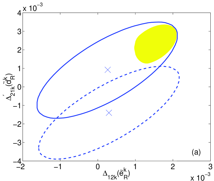
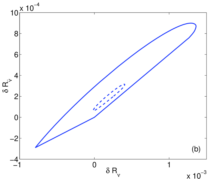
Figure 7: Plot(a) shows the 1 $\sigma$ allowed region in $\Delta_{12k}(\tilde{e}_{R}^{k})$-$\Delta_{21k}^{\prime}(\tilde{d}_{R}^{k})$ plane, with the best fit value denoted by the cross. The solid (dashed) ellipse is the fit excluding (including) the NuTeV $R_{\nu,\bar{\nu}}$ results. Shading indicates the physically allowed region, corresponding to $\Delta_{ijk}>0$ and $\Delta_{ijk}^{\prime}>0$. Plot(b) shows the prediction for $\delta R_{\nu}$ and $\delta R_{\bar{\nu}}$, using the 95$\%$ C.L. (solid line) or 1 $\sigma$ (dashed line) allowed values for $\Delta_{12k}(\tilde{e}_{R}^{k})$ and $\Delta_{21k}^{\prime}(\tilde{d}_{R}^{k})$ from fitting to $\delta|V_{ud}|^{2}/|V_{ud}|^{2}$, $\delta Q_{W}^{Cs}/Q_{W}^{Cs}$, $\delta R_{e/\mu}$ and $\delta G_{\mu}/G_{\mu}$ with $\Delta_{2k1}^{\prime}(\tilde{d}_{L}^{k})$ set to zero.

We also performed a fit to the five RPV parameters including in addition the NuTeV results for ${R_{\nu}}$ and ${R_{\bar{\nu}}}$. The one $\sigma$ allowed region for $\Delta_{12k}(\tilde{e}_{R}^{k})$ and $\Delta_{21k}^{\prime}(\tilde{d}_{R}^{k})$ is given by the dashed ellipse in Fig. 7 (a). At 95% C.L., at least one of the $\Delta_{ijk}^{(\prime)}$ must be negative in this fit. Thus, inclusion of the NuTeV results appears to exclude the RPV SUSY effects summarized in Table 2 with fairly high confidence.

V conclusion

The NuTeV anomaly remains in need of explanation. If one is ultimately unable to account for it with conventional, SM effects (e.g., small effects in parton distribution functions), then one would require an explanation lying outside the SM. Here, we have shown that such an explanation would be hard to come by in the MSSM alone. In general, SUSY loop corrections to ${R_{\nu}}$ and ${R_{\bar{\nu}}}$ generally have too small a magnitude and the wrong sign to account for the effect. An exception occurs for significant left-right mixing among first generation squarks, where a sizable effect of the necessary sign is generated by gluino loops. At present, precision data exclude this scenario with a high degree of confidence, though a new analysis of $K_{\ell 3}$ decays may weaken these restrictions considerably. Even in this case, however, the value for the weak mixing angle extracted from neutrino-nucleus scattering will be largely unaffected by gluino loops when a Paschos-Wolfenstein type relation is used for the extraction.

R parity-violating effects also appear at odds with the NuTeV anomaly. Inclusion of these effects could resolve an apparent conflict between tests of charged current universality and implications of SUSY-breaking models for the MSSM spectrumkurylov02 . However they would also render the LSP unstable and, therefore, rule out SUSY dark matter. At face value, the NuTeV results appear to disfavor this resolution of the charged current universality problem. In short, we conclude that the MSSM – with or without R-parity conservation – is likely not responsible for the NuTeV anomaly. The culprit, apparently, is to be found elsewhere.

Appendix A Essential Feynman rules

The complete set of Feynman rules for the MSSM can be found in haber ; rosiek . Here, we give only a brief list of relevant vertices.

The fermion-sfermion-gaugino vertices are:

where $e$ is the absolute value of the electron charge, $g_{S}$ is the ${\rm SU(3)}_{c}$ coupling constant, and $\lambda_{\alpha\beta}^{a}$ are Gell-Mann matrices rosiek , normalized according to $tr[\lambda^{a}\lambda^{b}]=1/2\delta^{ab}$. We use the capitalized letters $I$ and $J$ to denote the family index for quarks and leptons ($I,J=1,\cdots,3$), small letters $i$ and $j$ to denote the index for squarks and sleptons ($i,j=1,\cdots,6$ except for sneutrino, when $i,j=1,\cdots,3$), and small letters $p$ and $n$ to denote the index for the neutralinos ($p,n=1,\cdots,4$) and charginos ($p,n=1,2$). The index $a$ is reserved for the gluino index, $a=1,\cdots,8$.

The first vertex represents the coupling of the fermion $F_{J}$ to the sfermion $\tilde{F}^{\prime}_{i}$ and chargino $\chi_{p}^{+}$ (or its charge conjugation field $\chi_{p}^{+c}$ if $F=D,L$.). The chargino coupling constants $g^{F_{J}ip}_{L,R}$ for the quark sector are as follows (the repeated index is summed over):

$$g_{L}^{U_{J}ip} = -\frac{1}{s}V_{IJ}^{*}\left(Z^{Ii}_{D}U_{p1}^{*}-{m_{D_{I}}\over{\sqrt{2}M_{W}\cos\beta}}Z^{I+3,i}_{D}U_{p2}^{*}\right)$$

$$g_{R}^{U_{J}ip} = \frac{1}{s}V_{IJ}^{*}{m_{U_{I}}\over{\sqrt{2}M_{W}\sin\beta}}Z^{Ii}_{D}U_{p2}$$

$$g_{L}^{D_{J}ip} = -\frac{1}{s}V_{IJ}\left(Z^{*Ii}_{U}V_{p1}^{*}-{m_{U_{I}}\over{\sqrt{2}M_{W}\sin\beta}}Z^{*I+3,i}_{U}V_{p2}^{*}\right)$$

$$g_{R}^{D_{J}ip} = \frac{1}{s}V_{IJ}{m_{D_{I}}\over{\sqrt{2}M_{W}\cos\beta}}Z^{*Ii}_{U}V_{p2},$$ (29)

where $s$ ($c$) is the sine (cosine) of Weinberg angle, $V_{IJ}$ is the usual CKM matrix, $m_{U_{I}},m_{D_{I}}$ is the mass of “up” or “down” quark for generation I, $\tan\beta=v_{u}/v_{d}$ is the ratio of the expectation values of the Higgs scalars, $Z_{U,D}$ are the unitary 6$\times$6 mixing matrices for up and down squarks, respectively, that diagonalize full sfermion mass matrices, and $U$ and $V$ are the unitary mixing matrices that diagonalize the chargino mass matrix haber . In practical calculations masses of the first and second generation quarks can be neglected as they are much smaller than the mass of the $W$ boson. Similarly, for lepton sector,

$$g_{L}^{\nu_{J}ip} = -\frac{1}{s}\left(Z^{Ji}_{L}U_{p1}^{*}-{m_{L_{J}}\over{\sqrt{2}M_{W}\cos\beta}}Z^{J+3,i}_{L}U_{p2}^{*}\right)$$

$$g_{R}^{\nu_{J}ip} = 0$$

$$g_{L}^{L_{J}ip} = -\frac{1}{s}Z^{*Ji}_{\nu}V_{p1}^{*}$$

$$g_{R}^{L_{J}ip} = \frac{1}{s}{m_{L_{J}}\over{\sqrt{2}M_{W}\cos\beta}}Z^{*Ji}_{\nu}V_{p2},$$ (30)

Note that the mixing matrix for sneutrinos $Z_{\nu}$ is 3$\times$3 because in the MSSM neutrinos are purely left-handed.

The second vertex represents coupling of a fermion to a sfermion and a neutralino. The corresponding coupling constants $g_{0L,0R}^{F_{J}ip}$ for the fermion-sfermion-neutralino vertex are:

$$g_{0L}^{U_{J}ip} = -\frac{1}{\sqrt{2}sc}\left[Z^{*Ji}_{U}\left(N_{p2}^{*}c+{1\over 3}N_{p1}^{*}s\right)+{m_{U_{J}}\over{M_{Z}\sin\beta}}Z^{*J+3,i}_{U}N_{p4}^{*}\right]$$

$$g_{0R}^{U_{J}ip} = \frac{1}{\sqrt{2}c}\left({4\over 3}Z^{*J+3,i}_{U}N_{p1}-{{m_{U_{J}}}\over{M_{Z}\sin\beta}}Z^{*Ji}_{U}N_{p4}\right)$$

$$g_{0L}^{D_{J}ip} = \frac{1}{\sqrt{2}sc}\left[Z^{Ji}_{D}\left(N_{p2}^{*}c-{1\over 3}N_{p1}^{*}s\right)-{m_{D_{J}}\over{M_{Z}\cos\beta}}Z^{J+3,i}_{D}N_{p3}^{*}\right]$$

$$g_{0R}^{D_{J}ip} = -\frac{1}{\sqrt{2}c}\left[{2\over 3}Z^{J+3,i}_{D}N_{p1}+{{m_{D_{J}}}\over{M_{Z}\cos\beta}}Z^{Ji}_{D}N_{p3}\right)$$

$$g_{0L}^{\nu_{J}ip} = -\frac{1}{\sqrt{2}sc}Z^{*Ji}_{\nu}\left(N_{p2}^{*}c-N_{p1}^{*}s\right]$$

$$g_{0R}^{\nu_{J}ip} = 0$$

$$g_{0L}^{L_{J}ip} = \frac{1}{\sqrt{2}sc}\left[Z^{Ji}_{L}\left(N_{p2}^{*}c+N_{p1}^{*}s\right)-{m_{L_{J}}\over{M_{Z}\cos\beta}}Z^{J+3,i}_{L}N_{p3}^{*}\right]$$

$$g_{0R}^{L_{J}ip} = -\frac{1}{\sqrt{2}c}\left(2Z^{J+3,i}_{L}N_{p1}+{{m_{L_{J}}}\over{M_{Z}\cos\beta}}Z^{Ji}_{L}N_{p3}\right),$$ (31)

where $N$ is a 4$\times$4 mixing matrix that diagonalizes neutralino mass matrixhaber .

Finally, quark-squark-gluino (the third vertex) couplings $g_{GL,GR}^{F_{J}i}$ are:

$$g_{GL}^{U_{J}i}=-\sqrt{2}Z^{*Ji}_{U} g_{GR}^{U_{J}i}=\sqrt{2}Z^{*J+3,i}_{U}$$

$$g_{GL}^{D_{J}i}=-\sqrt{2}Z^{Ji}_{D} g_{GR}^{D_{J}i}=\sqrt{2}Z^{J+3,i}_{D}.$$ (32)

The gauge boson-gaugino-gaugino couplings are given as follows:

where

$$O^{L}_{pn}=\left(N_{p2}V^{*}_{n1}-{1\over{\sqrt{2}}}N_{p4}V^{*}_{n2}\right) O^{R}_{pn}=\left(N^{*}_{p2}U_{n1}+{1\over{\sqrt{2}}}N^{*}_{p3}U_{n2}\right)$$

$$O^{L\prime}_{pn}=\left(-V_{p1}V^{*}_{n1}-{1\over 2}V_{p2}V^{*}_{n2}+\delta_{pn}s^{2}\right) O^{R\prime}_{pn}=\left(-U^{*}_{p1}U_{n1}-{1\over 2}U^{*}_{p2}U_{n2}+\delta_{pn}s^{2}\right)$$

$$O^{L\prime\prime}_{pn}=\left(-{1\over 2}N_{p3}N^{*}_{n3}+{1\over 2}N_{p4}N^{*}_{n4}\right) O^{R\prime\prime}_{pn}=-O^{*L\prime\prime}_{pn}.$$ (33)

In addition, for the photon-chargino-chargino vertex $A^{\mu}-\chi_{n}^{+}-\chi_{p}^{+}$ is given by $-ie\gamma^{\mu}\delta^{pn}$.

The gauge boson-sfermion-sfermion vertices are given by:

For the $W$- coupling:

$$g_{W\tilde{D}_{i}\tilde{U}_{j}}=-\frac{1}{\sqrt{2}s}V_{JI}Z_{D}^{*Ii}Z_{U}^{*Jj},\ \ \ g_{W\tilde{L}_{i}\tilde{\nu}_{j}}=-\frac{1}{\sqrt{2}s}Z_{L}^{*Ii}Z_{\nu}^{*Jj}.$$ (34)

and for the $Z$ and $\gamma$ couplings:

$$g_{Z\tilde{F}_{i}\tilde{F}_{j}} = -\frac{1}{sc}\left(I_{3}^{F}Z_{F}^{Ii}Z_{F}^{*Ij}-Q_{F}s^{2}\delta_{ij}\right)$$

$$g_{\gamma\tilde{F}_{i}\tilde{F}_{j}} = -Q_{F}\delta^{ij}.$$ (35)

Here, $I_{3}^{F}$ and $Q_{F}$ are the isospin and the electric charge of the sfermions $\tilde{F}$, respectively.

The two scalar-two gauge boson vertices necessary for the calculation of the gauge boson self energies are (see Ref. rosiek ):

where

$$g_{WW\tilde{F}_{i}\tilde{F}_{j}} = \frac{1}{2s^{2}}Z_{F}^{Ki}Z_{F}^{*Kj}g^{\mu\nu}$$

$$g_{ZZ\tilde{F}_{i}\tilde{F}_{j}} = \frac{1}{s^{2}c^{2}}\left(2I_{3}^{F}(I_{3}^{F}-2Q_{F}s^{2})Z_{F}^{Ki}Z_{F}^{*Kj}+2Q_{F}^{2}s^{4}\delta_{ij}\right)g^{\mu\nu}$$

$$g_{Z\gamma\tilde{F}_{i}\tilde{F}_{j}} = \frac{1}{sc}Q_{F}\left(2I_{3}^{F}Z_{F}^{Ki}Z_{F}^{*Kj}-2Q_{F}s^{2}\delta_{ij}\right)g^{\mu\nu}$$

$$g_{\gamma\gamma\tilde{F}_{i}\tilde{F}_{j}} = 2Q_{F}^{2}\delta_{ij}g^{\mu\nu}.$$ (36)

Appendix B Expressions for the relevant Feynman diagrams

In this section, we list analytical expressions for the MSSM contribution to the gauge boson self-energies, the fermion wave function renormalization, the gauge boson-fermion-fermion vertex correction, and the box diagrams relevant to the neutrino-nucleus scatterings. Modified dimensional reduction (${\overline{DR}}$) scheme is used in computing MSSM loop contributions, although in the Appendices, we have neglected the hat in all relevant variables.

B.1 Gauge Boson Self-Energies

We first define the following class of two-point integration functions:

$$F_{n}(m_{1},m_{2},m_{3}) = {\int_{0}^{1}}x^{n}\ln\left\{\left[xm_{1}^{2}+(1-x)m_{2}^{2}-x(1-x)m_{3}^{2}\right]/\mu^{2}\right\},$$ (37)

$$F_{12}(m_{1},m_{2},m_{3}) = F_{1}(m_{1},m_{2},m_{3})-F_{2}(m_{1},m_{2},m_{3}),$$ (38)

where $\mu$ is the renormalization scale. In our analysis, $m_{3}^{2}$ will be replaced with either the external fermion mass squared or one of the Mandelstaam variables. For the first two generation quarks and the first two generation leptons the fermion mass can be set to zero. Focusing on the case when all Mandelstaam variables are small compared to $m_{1,2}^{2}$, we obtain:

$$F_{0}(m_{1},m_{2},0) = \ln m_{1}^{2}-1+{m_{2}^{2}\over{m_{2}^{2}-m_{1}^{2}}}\ln{m_{2}^{2}\over m_{1}^{2}}-\ln\mu^{2}$$

$$F_{1}(m_{1},m_{2},0) = {1\over 4}\Biggl{[}2\ln m_{1}^{2}-1+{2m_{2}^{2}\over{m_{1}^{2}-m_{2}^{2}}}+{2m_{2}^{4}\over{(m_{2}^{2}-m_{1}^{2})^{2}}}\ln{m_{2}^{2}\over m_{1}^{2}}-2\ln\mu^{2}\Biggr{]}.$$ (39)

B.1.1 Gaugino Loops

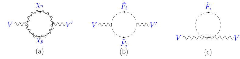
Figure 8: Feynman diagrams of one loop SUSY contributions to the gauge boson self energy.

The Feynman diagrams of this type are shown in Fig. 8(a). The contribution of gaugino loops to $W$ and $Z$ self-energies is given by

$$\Pi_{VV}^{\chi\chi}(q^{2}) = -{\alpha\over 2\pi}\sum_{p,n}\Biggl{\{}(g_{L}g_{R}^{*}+g_{L}^{*}g_{R})m_{\chi_{n}}m_{\chi_{p}}F_{0}(m_{\chi_{n}},m_{\chi_{p}},q)$$ (40)

$$+\left(|g_{L}|^{2}+|g_{R}|^{2}\right)\left[2q^{2}F_{12}(m_{\chi_{n}},m_{\chi_{p}},q)-m_{\chi_{n}}^{2}F_{1}(m_{\chi_{n}},m_{\chi_{p}},q)-m_{\chi_{p}}^{2}F_{1}(m_{\chi_{p}},m_{\chi_{n}},q)\right]\Biggr{\}},$$

where $q^{\mu}$ is the momentum carried by gauge boson $V$, and $q^{2}=q^{\mu}q_{\mu}$. The couplings $g_{L}$ and $g_{R}$ are listed below for $\Pi_{WW}$ and $\Pi_{ZZ}$:

$\Pi_{VV}$	$\chi_{p}$	$\chi_{n}$	$g_{L}$	$g_{R}$	comment
$\Pi_{WW}^{\chi^{0}\chi^{+}}$	$\chi^{0}_{p}$	$\chi^{+}_{n}$	$O^{L}_{pn}/s$	$O^{R}_{pn}/s$
$\Pi_{ZZ}^{\chi^{+}\chi^{+}}$	$\chi^{+}_{p}$	$\chi^{+}_{n}$	$O^{L\prime}_{pn}/sc$	$O^{R\prime}_{pn}/sc$
$\Pi_{ZZ}^{\chi^{0}\chi^{0}}$	$\chi^{0}_{p}$	$\chi^{0}_{n}$	$O^{L\prime\prime}_{pn}/sc$	$O^{R\prime\prime}_{pn}/sc$	multiply $1/2$

The $Z-\gamma$ mixing tensor and photon self-energy from chargino loops is given by

$$\Pi_{VV^{\prime}}^{\chi^{+}}(q^{2}) = -q^{2}{\alpha\over\pi}\sum_{p}g_{V}g_{V\prime}F_{12}(m_{\chi^{+}_{p}},m_{\chi^{+}_{p}},q),$$ (41)

with the couplings $g_{V}$ and $g_{V^{\prime}}$ listed below:

$\Pi_{VV^{\prime}}$	$g_{V}$	$g_{V\prime}$	comment
$\Pi_{Z\gamma}^{\chi^{+}}$	$(O^{L\prime}_{pp}+O^{R\prime}_{pp})/sc$	-1
$\Pi_{\gamma\gamma}^{\chi^{+}}$	-1	-1	multiply $2$

B.1.2 Scalar Loops

Diagrams of this type are shown in Figs. 8(b,c). The contribution of Fig. 8 (b) to $\Pi_{WW}$, $\Pi_{ZZ}$, $\Pi_{Z\gamma}$ and $\Pi_{\gamma\gamma}$ is given by

$$\Pi_{VV^{\prime}}^{{\tilde{F}}{\tilde{F}}}(q^{2}) = -{\alpha\over 4\pi}\sum_{i,j}g_{V\tilde{F}_{i}\tilde{F}_{j}}g_{V^{\prime}\tilde{F}_{i}\tilde{F}_{j}}^{*}\Biggl{\{}m_{{\tilde{F}}_{i}}^{2}+m_{{\tilde{F}}_{j}}^{2}-{q^{2}\over 3}$$ (42)

$$-2\Biggl{[}m_{{\tilde{F}}_{i}}^{2}F_{1}(m_{{\tilde{F}}_{i}},m_{{\tilde{F}}_{j}},q)+m_{{\tilde{F}}_{j}}^{2}F_{1}(m_{{\tilde{F}}_{j}},m_{{\tilde{F}}_{i}},q)-q^{2}F_{12}(m_{{\tilde{F}}_{i}},m_{{\tilde{F}}_{j}},q)\Biggr{]}\Biggr{\}}.$$

The sfermion pair $(\tilde{F}_{i},\tilde{F}_{j})$ running in the loop for $\Pi_{VV^{\prime}}$ is listed below:

$(V,V^{\prime})$	$(\tilde{F}_{i},\tilde{F}_{j})$
$(W,W)$	$(\tilde{L}_{i},\tilde{\nu}_{j})$, $(\tilde{D}_{i},\tilde{U}_{j})$
$(Z,Z)$	$(\tilde{\nu}_{i},\tilde{\nu}_{j})$, $(\tilde{L}_{i},\tilde{L}_{j})$, $(\tilde{U}_{i},\tilde{U}_{j})$ ,$(\tilde{D}_{i},\tilde{D}_{j})$
$(Z,\gamma)$	$(\tilde{L}_{i},\tilde{L}_{j})$, $(\tilde{U}_{i},\tilde{U}_{j})$ ,$(\tilde{D}_{i},\tilde{D}_{j})$
$(\gamma,\gamma)$	$(\tilde{L}_{i},\tilde{L}_{j})$, $(\tilde{U}_{i},\tilde{U}_{j})$ ,$(\tilde{D}_{i},\tilde{D}_{j})$

For squark contributions, an additional color factor of $N_{c}$ enters the right-hand side of Eq. (42).

The contribution of Fig. 8 (c) to the self-energies is given by

$$\Pi_{VV^{\prime}}^{{\tilde{F}}}(q^{2}) = {\alpha\over 4\pi}\sum_{i}g_{VV^{\prime}\tilde{F}_{i}\tilde{F}_{i}}m_{{\tilde{F}}_{i}}^{2}\left(1-\ln m_{{\tilde{F}}_{i}}^{2}+\ln\mu^{2}\right),$$ (43)

where $\tilde{F}=\tilde{\nu},\ \tilde{L},\tilde{U}$ and $\tilde{D}$ except for $V^{\prime}=\gamma$, for which $\tilde{\nu}$ does not contribute.

When $q^{2}\rightarrow 0$, $\Pi_{Z\gamma}(q^{2})/q^{2}$ and $\Pi_{\gamma\gamma}(q^{2})/q^{2}$ from sfermion loops reduce to

$$\frac{\Pi_{VV^{\prime}}(q^{2})}{q^{2}}=-\frac{\alpha}{12\pi}\sum_{i}g_{V\tilde{F}_{i}\tilde{F}_{i}}g_{V^{\prime}\tilde{F}_{i}\tilde{F}_{i}}^{*}\left(\ln m^{2}_{\tilde{F}_{i}}-\ln\mu^{2}\right).$$ (44)

B.2 Field Strength Renormalization for Fermions

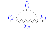
Figure 9: Feynman diagrams of one loop SUSY contribution to the fermion wave function renormalization.

The diagrams contributing to the field strength renormalization for fermions all have the form shown in Fig 9. Therefore, the same formula can be applied to contributions with charginos and neutralinos in the loop, provided that the appropriate couplings and masses are used. The gluino contributions are multiplied by an extra factor of Casimir factor $C_{2}(N)=4/3$ for ${\rm SU(3)}_{c}$. The field strength renormalization for the left-handed quark $F_{J}$ is

$$\delta Z^{F_{J}}_{L} = {{\alpha}\over{4\pi}}{\sum_{i,p}}{\left|g^{F_{J}ip}_{L}\right|}^{2}F_{1}(m_{{\tilde{F}^{\prime}}_{i}},m_{\chi^{+}_{p}},m_{F_{J}})+{{\alpha}\over{4\pi}}{\sum_{i,p}}{\left|g^{F_{J}ip}_{0L}\right|}^{2}F_{1}(m_{{\tilde{F}}_{i}},m_{\chi^{0}_{p}},m_{F_{J}})$$ (45)

$$+{4\over 3}\times{{\alpha_{S}}\over{4\pi}}{\sum_{i}}{\left|g^{F_{J}i}_{GL}\right|}^{2}F_{1}(m_{{\tilde{F}}_{i}},m_{\tilde{g}},m_{F_{J}}),$$

where $m_{\tilde{g}}$ is the gluino mass and $F^{\prime}$ stands for the isopartner of the fermion $F$ (e.g. if $F$ is the up-type quark, then $F^{\prime}$ is the down-type quark). By replacing $L\to R$ one easily obtains the field strength renormalization for the right-handed fermions. The same formulae apply to the sleptons provided that the appropriate couplings and masses are used. Naturally, corrections involving the strong coupling are absent in that case.

B.3 Vertex Corrections

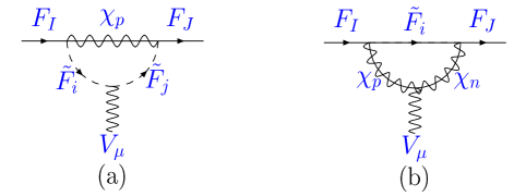
Figure 10: Feynman diagrams of one loop SUSY contribution to the gauge coupling vertex.

One-loop SUSY corrections to the $V-f-f^{\prime}$ vertex are shown in Fig. 10. There are two types of corrections: loops with the vector boson coupling to the scalar particles, Fig. 10(a), and loops with the vector bosons coupling to the gauginos, Fig. 10(b). The complete set of Feynman diagrams for each vertex, such as $W-d-u$, can contain more than one diagram of each type. However, since these diagrams differ only in the specific values of the masses and couplings needed to obtain the numerical answer we do not show all graphs explicitly. Below, we use the superscripts (a) and (b) to distinguish between the two types of loop graphs. To distinguish the graphs of the same type, we supplement the superscript with a number.

We first define the three-point integration functions needed for the evaluation of the triangle diagrams:

$$V_{1}(M,m_{1},m_{2}) = \int_{0}^{1}dx\int_{0}^{1}dy{y\over D_{3}(M,m_{1},m_{2})}$$

$$V_{2}(M,m_{1},m_{2}) = \int_{0}^{1}dx\int_{0}^{1}dy{y\ln\left[D_{3}(M,m_{1},m_{2})/\mu^{2}\right]}$$

$$D_{3}(M,m_{1},m_{2}) = (1-y)M^{2}+y[(1-x)m_{1}^{2}+xm_{2}^{2}].$$ (46)

Explicitly:

$$V_{1}(M,m_{1},m_{2}) = {{m_{1}^{2}\ln{m_{1}^{2}\over M^{2}}}\over{(M^{2}-m_{1}^{2})(m_{2}^{2}-m_{1}^{2})}}+{{m_{2}^{2}\ln{m_{2}^{2}\over M^{2}}}\over{(M^{2}-m_{2}^{2})(m_{1}^{2}-m_{2}^{2})}}$$

$$V_{2}(M,m_{1},m_{2}) = {1\over 4}\Biggl{[}2\ln{M^{2}}-3+{2m_{1}^{4}\over{(M^{2}-m_{1}^{2})(m_{2}^{2}-m_{1}^{2})}}\ln{m_{1}^{2}\over M^{2}}$$ (47)

$$+{2m_{2}^{4}\over{(M^{2}-m_{2}^{2})(m_{1}^{2}-m_{2}^{2})}}\ln{m_{2}^{2}\over M^{2}}-2\ln\mu^{2}\Biggr{]}.$$

Defining the matrix element for the vertex to be

$${\cal{M}}=ie[\delta_{VF_{I}F_{J}}^{L}{\bar{F}_{J}}\gamma^{\mu}P_{L}F_{I}+\delta_{VF_{I}F_{J}}^{R}{\bar{F}_{J}}\gamma^{\mu}P_{R}F_{I}]V_{\mu}.$$ (48)

Diagram (a) gives

$$\delta_{VF_{I}F_{J}}^{L;(a)} = -{{\alpha}\over{4\pi}}{\sum_{p,i,j}}g_{V\tilde{F}_{i}\tilde{F}_{j}}g_{\chi L}^{I}g_{\chi L}^{J*}V_{2}(m_{\chi_{p}},m_{{\tilde{F}}_{i}},m_{{\tilde{F}}_{j}})$$ (49)

$$\delta_{VF_{I}F_{J}}^{R;(a)} = -{{\alpha}\over{4\pi}}{\sum_{p,i,j}}g_{V\tilde{F}_{i}\tilde{F}_{j}}g_{\chi R}^{I}g_{\chi R}^{J*}V_{2}(m_{\chi_{p}},m_{{\tilde{F}}_{i}},m_{{\tilde{F}}_{j}}).$$ (50)

Diagram (b) gives

$$\delta_{VF_{I}F_{J}}^{L;(b)} = {{\alpha}\over{4\pi}}{\sum_{p,n,i}}\left[g_{V\chi\chi}^{L}g_{\chi L}^{I}g_{\chi L}^{J*}m_{\chi_{p}}m_{\chi_{n}}V_{1}-g_{V\chi\chi}^{R}g_{\chi L}^{I}g_{\chi L}^{J*}\left(1/2+V_{2}\right)\right]$$ (51)

$$\delta_{VF_{I}F_{J}}^{R;(b)} = {{\alpha}\over{4\pi}}{\sum_{p,n,i}}\left[g_{V\chi\chi}^{R}g_{\chi R}^{I}g_{\chi R}^{J*}m_{\chi_{p}}m_{\chi_{n}}V_{1}-g_{V\chi\chi}^{L}g_{\chi R}^{I}g_{\chi R}^{J*}\left(1/2+V_{2}\right)\right],$$ (52)

with the argument for functions $V$’s in Eqs. (51), (52) being $V_{1,2}(m_{\tilde{F}_{i}},m_{\chi_{p}},m_{\chi_{n}})$. The explicit expression for $g_{V\tilde{F}_{i}\tilde{F}_{j}}$, $g_{V\chi\chi}^{L,R}$, $g_{\chi L}^{I,J}$ and $g_{\chi R}^{I,J}$ for each individual vertex diagrams will be given below.

B.3.1 Charged Current Vertex

The vertex correction to $W-D_{I}-U_{J}$ is

$\delta_{VF_{I}F_{J}}^{(a)}$	$\chi_{p}$	$\tilde{F}_{i}$	$\tilde{F}_{j}$	$g_{V\tilde{F}_{i}\tilde{F}_{j}}$	$g_{\chi L,R}^{I}$	$g_{\chi L,R}^{J}$	$\delta_{VF_{I}F_{J}}^{(b)}$	$\chi_{p}$	$\chi_{n}$	$\tilde{F}_{i}$	$g_{V\chi\chi}^{L}$	$g_{V\chi\chi}^{R}$	$g_{\chi L,R}^{I}$	$g_{\chi L,R}^{J}$
$\delta_{WD_{I}U_{J}}^{(a1)}$	$\chi^{0}_{p}$	$\tilde{D}_{i}$	$\tilde{U}_{j}$	$g_{W\tilde{D}_{i}\tilde{U}_{j}}$	$g_{0L,R}^{D_{I}ip}$	$g_{0L,R}^{U_{J}jp}$	$\delta_{WD_{I}U_{J}}^{(b1)}$	$\chi^{0}_{p}$	$\chi^{+}_{n}$	$\tilde{D}_{i}$	$O_{pn}^{*L}/s$	$O_{pn}^{*R}/s$	$g_{0L,R}^{D_{I}ip}$	$g_{L,R}^{U_{J}in}$
							$\delta_{WD_{I}U_{J}}^{(b2)}$	$\chi^{+}_{p}$	$\chi^{0}_{n}$	$\tilde{U}_{i}$	$-O_{np}^{*R}/s$	$-O_{np}^{*L}/s$	$g_{L,R}^{D_{I}ip}$	$g_{0L,R}^{U_{J}in}$

The vertex correction due to gluino exchange is similar to $\delta_{WD_{I}U_{J}}^{(a1)}$, with the substitution of

$$\alpha\rightarrow\alpha_{S},\ \ \ \chi^{0}_{p}\rightarrow\tilde{g},\ \ \ g_{0L,R}^{D_{I}ip}\rightarrow g_{GL,R}^{D_{I}i},\ \ \ g_{0L,R}^{U_{J}jp}\rightarrow g_{GL,R}^{U_{J}j},\ \ \$$ (53)

and multiplication of the whole expression by 4/3. This substitution rule also applies for the neutral current vertex listed in the next section.

Similar to the case of the field strengths, the corresponding vertex corrections involving leptons $\delta_{VL_{I}\nu_{J}}$ are obtained from by using the appropriate masses and couplings. The gluino loop corrections must be omitted in that case.

B.3.2 Neutral Current Vertex

For the $Z-D_{I}-D_{J}$ vertex

$\delta_{VF_{I}F_{J}}^{(a)}$	$\chi_{p}$	$\tilde{F}_{i}$	$\tilde{F}_{j}$	$g_{V\tilde{F}_{i}\tilde{F}_{j}}$	$g_{\chi L,R}^{I}$	$g_{\chi L,R}^{J}$	$\delta_{VF_{I}F_{J}}^{(b)}$	$\chi_{p}$	$\chi_{n}$	$\tilde{F}_{i}$	$g_{V\chi\chi}^{L}$	$g_{V\chi\chi}^{R}$	$g_{\chi L,R}^{I}$	$g_{\chi L,R}^{J}$
$\delta_{ZD_{I}D_{J}}^{(a1)}$	$\chi^{0}_{p}$	$\tilde{D}_{i}$	$\tilde{D}_{j}$	$g_{Z\tilde{D}_{i}\tilde{D}_{j}}$	$g_{0L,R}^{D_{I}ip}$	$g_{0L,R}^{D_{J}jp}$	$\delta_{ZD_{I}D_{J}}^{(b1)}$	$\chi^{0}_{p}$	$\chi^{0}_{n}$	$\tilde{D}_{i}$	$O_{np}^{L\prime\prime}/sc$	$O_{np}^{R\prime\prime}/sc$	$g_{0L,R}^{D_{I}ip}$	$g_{0L,R}^{D_{J}in}$
$\delta_{ZD_{I}D_{J}}^{(a2)}$	$\chi^{+}_{p}$	$\tilde{U}_{i}$	$\tilde{U}_{j}$	$g_{Z\tilde{U}_{i}\tilde{U}_{j}}$	$g_{L,R}^{D_{I}ip}$	$g_{L,R}^{D_{J}jp}$	$\delta_{ZD_{I}D_{J}}^{(b2)}$	$\chi^{+}_{p}$	$\chi^{+}_{n}$	$\tilde{U}_{i}$	$-O_{pn}^{R\prime}/sc$	$-O_{pn}^{L\prime}/sc$	$g_{L,R}^{D_{I}ip}$	$g_{L,R}^{D_{J}in}$

For the $Z-U_{I}-U_{J}$ vertex

$\delta_{VF_{I}F_{J}}^{(a)}$	$\chi_{p}$	$\tilde{F}_{i}$	$\tilde{F}_{j}$	$g_{V\tilde{F}_{i}\tilde{F}_{j}}$	$g_{\chi L,R}^{I}$	$g_{\chi L,R}^{J}$	$\delta_{VF_{I}F_{J}}^{(b)}$	$\chi_{p}$	$\chi_{n}$	$\tilde{F}_{i}$	$g_{V\chi\chi}^{L}$	$g_{V\chi\chi}^{R}$	$g_{\chi L,R}^{I}$	$g_{\chi L,R}^{J}$
$\delta_{ZU_{I}U_{J}}^{(a1)}$	$\chi^{0}_{p}$	$\tilde{U}_{i}$	$\tilde{U}_{j}$	$g_{Z\tilde{U}_{i}\tilde{U}_{j}}$	$g_{0L,R}^{U_{I}ip}$	$g_{0L,R}^{U_{J}jp}$	$\delta_{ZU_{I}U_{J}}^{(b1)}$	$\chi^{0}_{p}$	$\chi^{0}_{n}$	$\tilde{U}_{i}$	$O_{np}^{L\prime\prime}/sc$	$O_{np}^{R\prime\prime}/sc$	$g_{0L,R}^{U_{I}ip}$	$g_{0L,R}^{U_{J}in}$
$\delta_{ZU_{I}U_{J}}^{(a2)}$	$\chi^{+}_{p}$	$\tilde{D}_{i}$	$\tilde{D}_{j}$	$g_{Z\tilde{D}_{i}\tilde{D}_{j}}$	$g_{L,R}^{U_{I}ip}$	$g_{L,R}^{U_{J}jp}$	$\delta_{ZU_{I}U_{J}}^{(b2)}$	$\chi^{+}_{p}$	$\chi^{+}_{n}$	$\tilde{D}_{i}$	$O_{np}^{L\prime}/sc$	$O_{np}^{R\prime}/sc$	$g_{L,R}^{U_{I}ip}$	$g_{L,R}^{U_{J}in}$

The radiative corrections to the lepton neutral current vertex are directly obtained from the above expressions by replacing the up (s)quark with the (s)neutrino and the down (s)quark with the (s)electron.

B.4 Anapole Moment Corrections

In the presence of parity-violating interactions, higher-order contributions can generate the photon-fermion-fermion coupling of the form (see, e.g. Ref. michael ):

$${\cal{L}}_{\gamma ff}^{PV}=-e\frac{F_{A,f}(q^{2})}{M_{Z}^{2}}\bar{f}(q^{2}\gamma^{\mu}-\not{\hbox{\kern-3.0pt$q$}}q^{\mu})\gamma_{5}fA_{\mu}.$$ (54)

The contributions from gaugino-sfermion loop at $q^{2}\rightarrow 0$ are:

$${F}_{A,f}(q^{2}) = {F}_{A,f}^{(a1)}(q^{2})+{F}_{A,f}^{(a2)}(q^{2})+{F}_{A,f}^{(b)}(q^{2})$$

$${F}_{A,f}^{(a1)}(q^{2}) = -Q_{f}{\alpha M_{Z}^{2}\over{48\pi}}\sum_{i,p}\left(|g_{0L}^{fip}|^{2}-|g_{0R}^{fip}|^{2}\right)\int_{0}^{1}{x^{3}dx\over{(1-x)m_{\chi^{0}_{p}}^{2}+xm_{{\tilde{f}}_{i}}^{2}}}$$

$${F}_{A,f}^{(a2)}(q^{2}) = -Q_{f^{\prime}}{\alpha M_{Z}^{2}\over{48\pi}}\sum_{i,p}\left(|g_{L}^{fip}|^{2}-|g_{R}^{fip}|^{2}\right)\int_{0}^{1}{x^{3}dx\over{(1-x)m_{\chi^{+}_{p}}^{2}+xm_{{\tilde{f}^{\prime}}_{j}}^{2}}}$$

$${F}_{A,f}^{(b)}(q^{2}) = 2I_{3}^{f}{\alpha M_{Z}^{2}\over{48\pi}}\sum_{i,p}\left(|g_{L}^{fip}|^{2}-|g_{R}^{fip}|^{2}\right)\int_{0}^{1}{x^{2}(x-3)dx\over{(1-x)m_{{\tilde{f}}_{i}}^{2}+xm_{\chi^{+}_{p}}^{2}}},$$ (55)

where $f^{\prime}$ stands for the isopartner of the fermion $f$ (e.g. if $f$ is the neutrino, then $f^{\prime}$ is the electron). Notice that for quark anapole moment, an additional gluino contribution should be added, when parity is broken in the presence of a non-zero left-right mixing in the squark sector and non-equal diagonal left and right squark masses. The gluino contribution can be obtained from ${F}_{A,f}^{(a1)}$ using the substitution rule give in Eq. (53). It should be remembered that the anapole moment of an elementary particle is not a physical observable michael . Here, we separate it from the other one-loop contributions purely for clarity of presentation.

B.5 Box Graphs

Let us introduce the following notation:

$$L(f^{\prime},f)_{\lambda} = {\bar{f}^{\prime}}(p^{\prime})\gamma_{\lambda}(1-\gamma_{5})f(p)$$

$$R(f^{\prime},f)_{\lambda} = {\bar{f}^{\prime}}(p^{\prime})\gamma_{\lambda}(1+\gamma_{5})f(p),$$ (56)

where $p$ and $p^{\prime}$ are the momenta of the incoming particle $f$ and outgoing $f^{\prime}$, respectively.

The four-point integration functions are defined as:

$$B_{1}(M_{1},M_{2},m_{1},m_{2}) = {\int_{0}^{1}dx}{\int_{0}^{1}dy}{\int_{0}^{1}dz}{{z(1-z)}\over D_{4}(M_{1},M_{2},m_{1},m_{2})}$$

$$B_{2}(M_{1},M_{2},m_{1},m_{2}) = {\int_{0}^{1}dx}{\int_{0}^{1}dy}{\int_{0}^{1}dz}{{z(1-z)}\over D_{4}^{2}(M_{1},M_{2},m_{1},m_{2})}$$

$$D_{4}(M_{1},M_{2},m_{1},m_{2}) = z[(1-x)M_{1}^{2}+xM_{2}^{2}]+(1-z)[(ym_{1}^{2}+(1-y)m_{2}^{2}].$$ (57)

The explicit formulae for $B_{1}$ and $B_{2}$ are

$$B_{1}(M_{1},M_{2},m_{1},m_{2})={m_{1}^{4}\ln{m_{1}^{2}\over M_{2}^{2}}\over{2(m_{1}^{2}-M_{1}^{2})(m_{1}^{2}-m_{2}^{2})(m_{1}^{2}-M_{2}^{2})}}$$

$$+{m_{2}^{4}\ln{m_{2}^{2}\over M_{2}^{2}}\over{2(m_{2}^{2}-m_{1}^{2})(m_{2}^{2}-M_{1}^{2})(m_{2}^{2}-M_{2}^{2})}}+{M_{1}^{4}\ln{M_{1}^{2}\over M_{2}^{2}}\over{2(M_{1}^{2}-m_{1}^{2})(M_{1}^{2}-m_{2}^{2})(M_{1}^{2}-M_{2}^{2})}}$$

$$B_{2}(M_{1},M_{2},m_{1},m_{2})={m_{1}^{2}\ln{M_{2}^{2}\over m_{1}^{2}}\over{(m_{1}^{2}-M_{1}^{2})(m_{1}^{2}-m_{2}^{2})(m_{1}^{2}-M_{2}^{2})}}$$

$$+{m_{2}^{2}\ln{M_{2}^{2}\over m_{2}^{2}}\over{(m_{2}^{2}-m_{1}^{2})(m_{2}^{2}-M_{1}^{2})(m_{2}^{2}-M_{2}^{2})}}+{M_{1}^{2}\ln{M_{2}^{2}\over M_{1}^{2}}\over{(M_{1}^{2}-m_{1}^{2})(M_{1}^{2}-m_{2}^{2})(M_{1}^{2}-M_{2}^{2})}}.$$ (58)

B.5.1 Charged Current Box

We define the matrix element of the box diagram as

$${\cal{M}}_{box}^{CC}=-i\frac{G_{\mu}}{\sqrt{2}}\delta_{B}^{CC}L(\mu,\nu_{\mu})_{\lambda}\times L(u,d)^{\lambda}+\ldots$$ (59)

to factor out the overall Fermi-constant. The dots denote other Dirac structures appearing in the amplitude that make negligible contributions (suppressed by $m_{\mu}$) to the total cross-section.

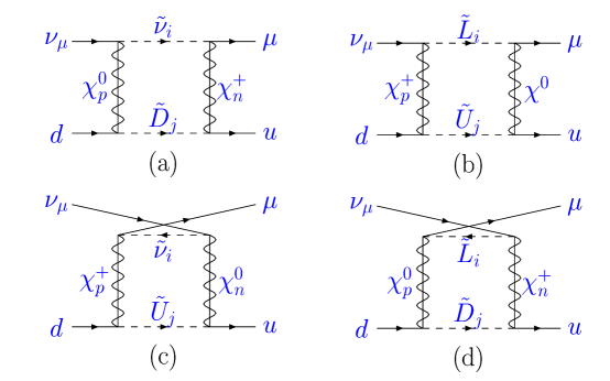
Figure 11: Feynman diagrams of one loop SUSY contribution to neutrino charge current box diagram.

For the graphs in Fig. 11 we have: $\delta_{B}^{CC}=\delta_{B}^{CC;a}+\delta_{B}^{CC;b}+\delta_{B}^{CC;c}+\delta_{B}^{CC;d}$

$$\delta_{B}^{CC;a} = -{\alpha M_{W}^{2}s^{2}\over{4\pi}}{\sum_{p,n,i,j}}g_{0L}^{\nu_{\mu}ip}g_{L}^{*\mu in}g_{0L}^{djp}g_{L}^{*ujn}m_{\chi^{0}_{p}}m_{\chi^{+}_{n}}B_{2}(m_{{\tilde{\nu}}_{i}},m_{{\tilde{D}}_{j}},m_{\chi^{0}_{p}},m_{\chi^{+}_{n}})$$

$$\delta_{B}^{CC;b} = -{\alpha M_{W}^{2}s^{2}\over{4\pi}}{\sum_{p,n,i,j}}g_{L}^{{\nu_{\mu}}ip}g_{0L}^{*\mu in}g_{L}^{djp}g_{0L}^{*ujn}m_{\chi^{+}_{p}}m_{\chi^{0}_{n}}B_{2}(m_{{\tilde{L}}_{i}},m_{{\tilde{U}}_{j}},m_{\chi^{+}_{p}},m_{\chi^{0}_{n}})$$

$$\delta_{B}^{CC;c} = {\alpha M_{W}^{2}s^{2}\over{4\pi}}{\sum_{p,n,i,j}}g_{0L}^{{\nu_{\mu}}in}g_{L}^{*\mu ip}g_{L}^{djp}g_{0L}^{*ujn}B_{1}(m_{{\tilde{\nu}}_{i}},m_{{\tilde{U}}_{j}},m_{\chi^{+}_{p}},m_{\chi^{0}_{n}})$$

$$\delta_{B}^{CC;d} = {\alpha M_{W}^{2}s^{2}\over{4\pi}}{\sum_{p,n,i,j}}g_{L}^{{\nu_{\mu}}in}g_{0L}^{*\mu ip}g_{0L}^{djp}g_{L}^{*ujn}B_{1}(m_{{\tilde{L}}_{i}},m_{{\tilde{D}}_{j}},m_{\chi^{0}_{p}},m_{\chi^{+}_{n}}).$$ (60)

Similarly, the box diagram contributing to the muon decay $\mu\rightarrow\nu_{\mu}e\bar{\nu}_{e}$ can be obtained from $\delta_{B}^{CC}$ using the substitution:

$$\delta_{B}^{CC}\rightarrow\delta_{B}^{\mu*},\ \ d\rightarrow e,\ \ u\rightarrow\nu_{e},\ \ \tilde{D}_{j}\rightarrow\tilde{L}_{j},\ \ \tilde{U}_{j}\rightarrow\tilde{\nu}_{j},\ \$$

$$g_{L,R,0L,0R}^{djp}\rightarrow g_{L,R,0L,0R}^{ejp},\ \ g_{L,R,0L,0R}^{ujn}\rightarrow g_{L,R,0L,0R}^{\nu_{e}jn}.$$ (61)

B.5.2 Neutral Current Box

We define the matrix element of the neutral current box diagram as

$${\cal{M}}_{box}^{NC}=-i\frac{G_{\mu}}{\sqrt{2}}\left[\delta_{B}^{L;q}L(\mu,\nu_{\mu})_{\lambda}\times L(q,q)^{\lambda}+\delta_{B}^{R;q}L(\mu,\nu_{\mu})_{\lambda}\times R(q,q)^{\lambda}\right].$$ (62)

The explicit expressions for the $\nu_{\mu}-q$ box graphs are given below.

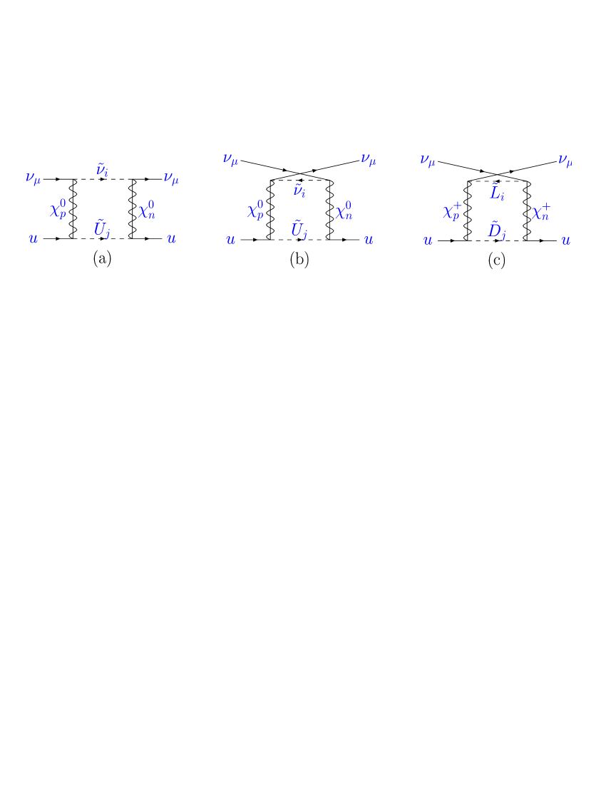
Figure 12: Feynman diagrams of one loop SUSY contribution to $\nu_{\mu}-u$ neutrino neutral current box diagram.

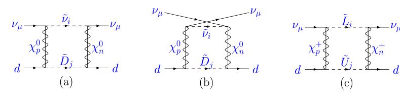
Figure 13: Feynman diagrams of one loop SUSY contribution to $\nu_{\mu}-d$ neutrino neutral current box diagram.

Up-quark box diagrams (Fig. 12): $\delta_{B}^{L;u}=\delta_{B}^{L;(u,a)}+\delta_{B}^{L;(u,b)}+\delta_{B}^{L;(u,c)}$, $\delta_{B}^{R;u}=\delta_{B}^{R;(u,a)}+\delta_{B}^{R;(u,b)}$,

$$\delta_{B}^{L;(u,a)}(NC) = -{\alpha M_{W}^{2}s^{2}\over{4\pi}}{\sum_{p,n,i,j}}g_{0L}^{\nu_{\mu}ip}g_{0L}^{*\nu_{\mu}in}g_{0L}^{ujp}g_{0L}^{*ujn}m_{\chi^{0}_{p}}m_{\chi^{0}_{n}}B_{2}(m_{{\tilde{\nu}}_{i}},m_{{\tilde{U}}_{j}},m_{\chi^{0}_{p}},m_{\chi^{0}_{n}})$$

$$\delta_{B}^{R;(u,a)}(NC) = -{\alpha M_{W}^{2}s^{2}\over{4\pi}}{\sum_{p,n,i,j}}g_{0L}^{\nu_{\mu}ip}g_{0L}^{*\nu_{\mu}in}g_{0R}^{ujp}g_{0R}^{*ujn}B_{1}(m_{{\tilde{\nu}}_{i}},m_{{\tilde{U}}_{j}},m_{\chi^{0}_{p}},m_{\chi^{0}_{n}})$$

$$\delta_{B}^{L;(u,b)}(NC) = {\alpha M_{W}^{2}s^{2}\over{4\pi}}{\sum_{p,n,i,j}}g_{0L}^{\nu_{\mu}in}g_{0L}^{*\nu_{\mu}ip}g_{0L}^{ujp}g_{0L}^{*ujn}B_{1}(m_{{\tilde{\nu}}_{i}},m_{{\tilde{U}}_{j}},m_{\chi^{0}_{p}},m_{\chi^{0}_{n}})$$

$$\delta_{B}^{R;(u,b)}(NC) = {\alpha M_{W}^{2}s^{2}\over{4\pi}}{\sum_{p,n,i,j}}g_{0L}^{\nu_{\mu}in}g_{0L}^{*\nu_{\mu}ip}g_{0R}^{ujp}g_{0R}^{*ujn}m_{\chi^{0}_{p}}m_{\chi^{0}_{n}}B_{2}(m_{{\tilde{\nu}}_{i}},m_{{\tilde{U}}_{j}},m_{\chi^{0}_{p}},m_{\chi^{0}_{n}})$$

$$\delta_{B}^{L;(u,c)}(NC) = {\alpha M_{W}^{2}s^{2}\over{4\pi}}{\sum_{p,n,i,j}}g_{L}^{\nu_{\mu}in}g_{L}^{*\nu_{\mu}ip}g_{L}^{ujp}g_{L}^{*ujn}B_{1}(m_{{\tilde{L}}_{i}},m_{{\tilde{D}}_{j}},m_{\chi^{+}_{p}},m_{\chi^{+}_{n}}).$$ (63)

Down-quark box diagrams (Fig. 12): $\delta_{B}^{L;d}=\delta_{B}^{L;(d,a)}+\delta_{B}^{L;(d,b)}+\delta_{B}^{L;(d,c)}$, $\delta_{B}^{R;d}=\delta_{B}^{R;(d,a)}+\delta_{B}^{R;(d,b)}$,

$$\delta_{B}^{L;(d,a)}(NC) = -{\alpha M_{W}^{2}s^{2}\over{4\pi}}{\sum_{p,n,i,j}}g_{0L}^{\nu_{\mu}ip}g_{0L}^{*\nu_{\mu}in}g_{0L}^{djp}g_{0L}^{*djn}m_{\chi^{0}_{p}}m_{\chi^{0}_{n}}B_{2}(m_{{\tilde{\nu}}_{i}},m_{{\tilde{D}}_{j}},m_{\chi^{0}_{p}},m_{\chi^{0}_{n}})$$

$$\delta_{B}^{R;(d,a)}(NC) = -{\alpha M_{W}^{2}s^{2}\over{4\pi}}{\sum_{p,n,i,j}}g_{0L}^{\nu_{\mu}ip}g_{0L}^{*\nu_{\mu}in}g_{0R}^{djp}g_{0R}^{*djn}B_{1}(m_{{\tilde{\nu}}_{i}},m_{{\tilde{D}}_{j}},m_{\chi^{0}_{p}},m_{\chi^{0}_{n}})$$

$$\delta_{B}^{L;(d,b)}(NC) = {\alpha M_{W}^{2}s^{2}\over{4\pi}}{\sum_{p,n,i,j}}g_{0L}^{\nu_{\mu}in}g_{0L}^{*\nu_{\mu}ip}g_{0L}^{djp}g_{0L}^{*djn}B_{1}(m_{{\tilde{\nu}}_{i}},m_{{\tilde{D}}_{j}},m_{\chi^{0}_{p}},m_{\chi^{0}_{n}})$$

$$\delta_{B}^{R;(d,b)}(NC) = {\alpha M_{W}^{2}s^{2}\over{4\pi}}{\sum_{p,n,i,j}}g_{0L}^{\nu_{\mu}in}g_{0L}^{*\nu_{\mu}ip}g_{0R}^{djp}g_{0R}^{*djn}m_{\chi^{0}_{p}}m_{\chi^{0}_{n}}B_{2}(m_{{\tilde{\nu}}_{i}},m_{{\tilde{D}}_{j}},m_{\chi^{0}_{p}},m_{\chi^{0}_{n}})$$

$$\delta_{B}^{L;(d,c)}(NC) = -{\alpha M_{W}^{2}s^{2}\over{4\pi}}{\sum_{p,n,i,j}}g_{L}^{\nu_{\mu}ip}g_{L}^{*\nu_{\mu}in}g_{L}^{djp}g_{L}^{*djn}m_{\chi^{+}_{p}}m_{\chi^{+}_{n}}B_{2}(m_{{\tilde{L}}_{i}},m_{{\tilde{U}}_{j}},m_{\chi^{+}_{p}},m_{\chi^{+}_{n}}).\ \ \$$ (64)

Appendix C radiative correction to neutrino-nucleus interactions

Given the expressions for the fermion field strength renormalization $\delta Z_{L,R}^{F_{I}}$, vertex correction $\delta_{VF_{I}F_{J}}^{L,R}$ and box diagrams $\delta_{B}^{L,R}$, $\delta_{VB}^{CC}$ in Eq. (8), $\delta_{V}^{\nu}$ in Eq. (9) and $\delta_{VB}^{L,R;q}$ in Eq. (11) can be expressed as

$$\delta_{VB}^{\mu} = \frac{1}{2}\left(\delta Z_{L}^{\mu}+\delta Z_{L}^{\nu_{\mu}}+\delta Z_{L}^{e}+\delta Z_{L}^{\nu_{e}}\right)-\sqrt{2}s\left(\delta_{W\nu_{e}e}^{L}+\delta_{W\mu\nu_{\mu}}^{L}\right)+\delta_{B}^{\mu}$$ (65)

$$\delta_{VB}^{CC} = \frac{1}{2}\left(\delta Z_{L}^{\nu_{\mu}}+\delta Z_{L}^{\mu}+\delta Z_{L}^{u}+\delta Z_{L}^{d}\right)-\sqrt{2}s\left(\delta_{W\nu_{\mu}\mu}^{L}+\delta_{Wdu}^{L}\right)+\delta_{B}^{CC}$$ (66)

$$\delta_{V}^{\nu} = \delta Z_{L}^{\nu_{\mu}}-2sc\ \delta_{Z\nu_{\mu}\nu_{\mu}}^{L}$$ (67)

$$\delta_{VB}^{L;q=u,d} = \frac{1}{2}\delta Z_{L}^{q}-sc\ \delta_{Zqq}^{L}+\delta_{B}^{L;q}$$ (68)

$$\delta_{VB}^{R;q=u,d} = \frac{1}{2}\delta Z_{R}^{q}-sc\ \delta_{Zqq}^{R}+\delta_{B}^{R;q}.$$ (69)

The neutrino anapole moment contribution to the neutral current neutrino-nucleus scattering is shown in Fig. 1(b), which is absorbed into $\delta\kappa_{\nu}$ as

$$\delta\kappa=-4c^{2}{F}_{A,\nu}(q^{2}).$$ (70)

References

- (1) G.P. Zeller, et al., the NuTeV Collaboration, Phys. Rev. Lett. 88, 091802 (2002).
- (2) Review of Particle Properties, Phys. Rev. D 66, 010001 (2002).
- (3) J. Erler, private communication.
- (4) S.C. Bennett and C.E. Wieman, Phys. Rev. Lett. 82, 2484 (1999); V.A. Dzuba, V.V. Flambaum, and J. S. M. Ginges, Phys. Rev. D 66:076013 (2002); A.I. Milstein, O.P. Sushkov, and I.S. Terekhov, hep-ph/0212072.
- (5) SLAC Experiment E-158, E.W. Hughes, K. Kumar, and P.A. Souder, spokespersons.
- (6) Jefferson Lab Experiment E-02-020, R. Carlini, J.M. Finn, S. Kowalski, and S. Page, spokespersons.
- (7) G.A. Miller and A.W. Thomas, hep-ex/0204007; see also K.S. McFarland, hep-ex/021001.
- (8) S. Davidson, et al., JHEP 02, 037 (2002).
- (9) A. Kurylov and M.J. Ramsey-Musolf, Phys. Rev. Lett. 88, 071804, 2002.
- (10) A. Kurylov, M.J. Ramsey-Musolf, and S. Su, hep-ph/0205183.
- (11) See, e.g., D.M. Pierce, hep-ph/9805497.
- (12) M. J. Ramsey-Musolf, Phys. Rev. D 62, 056009 (2000).
- (13) H. E. Haber and G. L. Kane, Phys. Rep. 117, 74 (1985).
- (14) M. E. Peskin and T. Takeuchi, Phys. Rev. Lett. 65, 964, 1990; Phys. Rev. D 46, 381, 1992.
- (15) G.W. Bennett, et al., Muon g-2 Collaboration, Phys. Rev. Lett. 89:101804 (2002).
- (16) A. Sher, talk given at the Institute for Nuclear Theory, Seattle, December 2002.
- (17) E. A. Paschos and L. Wolfenstein, Phys. Rev. D 7, 91 (1973).
- (18) H. Schellman, private communication.
- (19) I. S. Towner and J. C. Hardy, Proceedings of the Fifth International WEIN Symposium: Physics Beyond the Standard Model, P. Herczeg, et al., eds. (World Scientific, 1999) p. 338.
- (20) G. Czapek et al., Phys. Rev. Lett. 70, 17 (1993); D. I. Britton, et al., Phys. Rev. Lett. 68, 3000 (1992).
- (21) W. J. Marciano, Phys. Rev. D 60:093006 (1999).
- (22) J. Rosiek, Phy. Rev. D 41, 3464, 1990.
- (23) M. J. Musolf, B. R. Holstein, Phys. Rev. D 43, 2956, 1991.