AS-ITP-2003-001

Diffractive Photoproduction of $\eta_{c}$

J. P. Ma

Institute of Theoretical Physics , Academia Sinica, Beijing 100080, China

Abstract

Diffractive photoproduction of $\eta_{c}$ is an important process to study the effect of Odderon, whose existence is still not confirmed in experiment. A detailed interpretation of Odderon in QCD, i.e., in terms of gluons is also unclear. Taking charm quarks as heavy quarks, we can use NRQCD and take $\eta_{c}$ as a $c\bar{c}$ bound state. Hence, in the production of $\eta_{c}$ a free $c\bar{c}$ pair is first produced and this pair is transformed into $\eta_{c}$ subsequently. In the forward region of the kinematics, the $c\bar{c}$ pair interacts with initial hadron through exchanges of soft gluons. This interaction can be studied with HQET, which provides a systematic expansion in the inverse of the $c$-quark mass $m_{c}$. We find that the calculation of the $S$-matrix element in the forward region can be formulated as the problem of solving a wave function of a $c$-quark propagating in a background field of soft gluons. At leading order we find that the differential cross-section can be expressed with four functions, which are defined with a twist-3 operator of gluons. The effect of exchanging a Odderon can be identified with this operator in our case. We discuss our results in detail and compare them with those obtained in previous studies. Our results and those from other studies show that the differential cross-section is very small in the forward region. We also show that the production through photon exchange is dominant in the extremely forward region, hence the effect of Odderon exchange can not be identified in this region. For completeness we also give results for diffractive photoproduction of $J/\Psi$.

PACS numbers: 12.38.-t, 12.39.Hg, 13.60.-r, 13.60.Le

Key Words: Soft gluon, HQET, diffractive photoproduction of $\eta_{c}$, HERA experiment.

1. Introduction

Diffractive photoproduction of a pseudoscalar meson is an interesting process because the production is related to the postulated object: Odderon[1], the partner of Pomeron. The Pomeron is even under charge conjugation $C$, while the Odderon has $C=-1$. The exchange of Pomeron and Odderon is believed to delivery dominant contributions to hadronic cross section at high energy. An interesting review about the history of Odderon and relevant references can be found in [2]. Giving the importance of its existence in theory, experimentally it is still unsuccessful to hunt the effect induced by Odderon. Only one indication for existence of Odderon is found in the $t$-dependence of $pp$- and $p\bar{p}$ elastic cross-section[3]. Theoretically the effect of Odderon exchange in $pp$- and $p\bar{p}$ scattering at high energy has been intensively studied, a recent work and useful references can be found in [4].

It has been suggested that the effect of Odderon may be detected in diffractive pseudoscalar meson production for collision of a hadron with a real- or virtual photon[5, 6, 7, 9, 10, 11], where effects of Pomeron are absent. It is difficult to made predictions for the proposed processes by starting from QCD directly. Some models are introduced to make predictions for the $ep$ collider at HERA. Unfortunately, the experimental study in photoproduction of $\pi^{0}$[12] gives a negative result. In [8] it is suggested to look for Odderon in productions of two pions. In [9, 10, 11] diffractive photoproduction of $\eta_{c}$ are studied, predictions may be made more reliably than those for production of light meson, because of the following reasons: The structure of $\eta_{c}$ is simpler than light mesons, the large quark mass $m_{c}$ enables us to use perturbative QCD at certain level and the $c$-quark content in the initial hadron can be neglected. Therefore the production of $\eta_{c}$ can be imagined as that the initial photon is split into a $c\bar{c}$ pair, this pair exchanges gluons with the initial hadron $h$ and forms the produced $\eta_{c}$ after exchanges. This is illustrated in Fig.1. Effect of exchanging gluons can be thought as the effect of exchanging a Odderon. In [9, 10] one uses perturbative QCD to handle the emission of gluons by the $c\bar{c}$ pair, at leading order only three gluons are emitted. The interaction of the three gluons with the initial hadron $h$ is described by a impact factor. Using models for the impact factor one can obtain some numerical predictions. In [11] one uses a set of new Odderon states to account the effect of Odderon exchange and numerical predictions can also be made. All of these works deliveries a total cross-section for HERA roughly at order of $10^{2}$pb, but the $t$-dependence is predicted differently in different works.

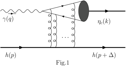
Figure 1: Typical diagram for exchange of many soft gluons for $\eta_{c}$ photoproduction

In this work we study the problem from another point of view. We make an attempt to answer the question if one can express the differential cross-section in the nearly forward direction with quantities which are well defined in the framework of QCD. The answer is closely related to a QCD interpretation of Odderon in our case. If $\eta_{c}$ is produced diffractively and the beam energies are large enough, the exchanged gluons are soft. It is questionable to use perturbative QCD for these soft gluons. But, the charm quark can be taken as a heavy quark, the emission of these soft gluons can be studied with the Heavy Quark Effective Theory(HQET)[13], in which a systematical expansion in $m_{c}^{-1}$ can be made. Also by taking charm quark as a heavy quark one can describe $\eta_{c}$ with nonrelativistic QCD(NRQCD)[14], in which a systematic expansion in the small velocity $v_{c}$, which is the velocity of a $c$- or $\bar{c}$ quark inside a charmonium in its rest frame, can be made. At leading order of $v_{c}$ the $c\bar{c}$ pair after exchanging soft gluons can be taken as on-shell. Using this fact, the study of the emission of soft gluons by the $c$- or $\bar{c}$ quark can be formulated to solve a wave function of the $c$- or $\bar{c}$ quark propagating in a background field of soft gluons. The problem of light quarks propagating in a background field of soft gluons have been studied in [15] in relation to hadron-hadron scattering at high energy. In our case these wave functions can be solved by expanding them in $m_{c}^{-1}$. It is interesting to note that at the limit $m_{c}\rightarrow\infty$ the exchanged Odderon here consists of three soft gluons but in a special gauge.

The approach outlined above has been used to study similar cases with exchanges of soft gluons like $J/\Psi\rightarrow\gamma^{*}+{\rm soft\ pions}$[16, 17] and diffractive photoproduction of $J/\Psi$[18]. In [18] it is assumed that results for the $S$-matrix element can be obtained by taking two-gluon exchange in a special gauge. In this work we derive these results for completeness and without the assumption. It shows that for the case of $J/\Psi$ the exchanging Pomeron consists of two gluons in this special gauge.

In this work we are unable to give numerical results in detail, because the differential cross-section is expressed with four unknown functions, which are defined with a twist-3 gluonic operator in QCD. However, order of magnitude can be estimated in comparison with the case of $J/\Psi$. It turns out that the differential cross-section is very small as that predicted by model calculations[9, 10, 11]. With our result it can be show that the differential cross-section can be non zero in the limit $t\rightarrow 0$, in contrast to the predicted in [9, 10, 11], where $t$ is the squared momentum transfer between light hadrons. The reason for this is that there are nonperturbative effects which can cause the helicity flip of the initial hadron. This will be discussed in detail. Since the differential cross-section with exchanges of soft gluons is small, the exchange of a photon, instead of exchanging many gluons in Fig.1., can have a sizeable contribution. At first look, the amplitude with exchange of a photon is divergent in the limit $t\rightarrow 0$. It should be noted that for large and finite $s$ the minimum of $|t|$ is small but not exactly zero. This fact makes the amplitude finite, it leads to that the differential cross-section in the forward direction increases linearly with $s$ and can be determined completely. We find that at energies relevant to HERA the contribution from photon exchange is actually dominant in the extremely forward direction. This may exclude the possibility to observe effect of Odderon exchange in this kinematical region. However, the contribution from photon exchange decreases with increasing $|t|$ more rapidly than that of Odderon exchange, it is possible to identify Odderon exchange at $|t|$ which is not very close to its minimal value.

Our work is organized as the following: In Sect.2. we use NRQCD factorization for $\eta_{c}$ and then formulate the problem of calculating the $S$-matrix element as the problem of solving wave functions of $c$ quarks in a background field of soft gluons. In Sect.3. we solve the wave functions by expanding them in $m_{c}^{-1}$. The relevant part of solutions are given. In Sect.4. we use these solutions to derive the $S$-matrix element for diffractive photoproduction of $J/\Psi$. The results derived in this way are exactly the same as those derived by the assumption of two-gluon exchange in a special gauge[18]. In Sect.5. we derive the results for $\eta_{c}$ production and discuss our results. In Sect.6. we study the contribution through exchange of a photon. Sect.7. is our summary.

2. Soft gluon exchange

We consider the diffractive process:

$$\gamma(q)+h(p)\rightarrow h(p+\Delta)+\eta_{c}(k)$$ (1)

where the momenta are indicated in the brackets and $k=q-\Delta$. The Mandelstam variables are defined as $s=(q+p)^{2}$ and $t=\Delta^{2}$. We consider the kinematic region where $|t|$ is at order of $\Lambda_{QCD}^{2}$ and each component of $\Delta$ is at order of $\Lambda_{QCD}$. The initial photon is real with $q^{2}=0$, $h$ is any light hadron whose mass $m$ is at order of $\Lambda_{QCD}$. Throughout this work we take nonrelativistic normalization for $\eta_{c}$ and $c$-quark. The process undergoes like that the initial photon first splits into a $c\bar{c}$ pair, this pair exchanges soft gluons with the light hadron and forms $\eta_{c}$ after the exchanges. A typical diagram for this is given in Fig.1. The $S$-matrix element can be written as a sum over contributions with $n$-gluon exchange:

$$\langle f|S|i\rangle = (2\pi)^{4}\delta^{4}(q-\Delta-k)\sum_{n}\frac{1}{n!}\int d^{4}x_{1}d^{4}x_{2}\cdots d^{4}x_{n}d^{4}x\int\frac{d^{4}k_{1}}{(2\pi)^{4}}\frac{d^{4}k_{2}}{(2\pi)^{4}}\cdots\frac{d^{4}k_{n}}{(2\pi)^{4}}\frac{d^{4}q_{1}}{(2\pi)^{4}}$$ (2)

$$\cdot A_{ij}^{a_{1}a_{2}\cdots a_{n},\mu_{1}\mu_{2}\cdots\mu_{n}}(q,q_{1},k_{1},k_{2},\cdots k_{n})e^{-iq_{1}\cdot x}\langle\eta_{c}(k)|\bar{c}_{i}(x)c_{j}(0)|0\rangle$$

$$\cdot e^{ik_{1}\cdot x_{1}+\cdots ik_{n}\cdot x_{n}}\langle h(p+\Delta)|G_{\mu_{1}}^{a_{1}}(x_{1})G_{\mu_{2}}^{a_{2}}(x_{2})\cdots G_{\mu_{n}}^{a_{n}}(x_{n})|h(p)\rangle,$$

where $i$ and $j$ stand for color- and Dirac indices for the Dirac fields $\bar{c}(x)$ and $c(0)$ respectively. $A_{ij}^{a_{1}a_{2}\cdots a_{n},\mu_{1}\mu_{2}\cdots\mu_{n}}(q,q_{1},k_{1},k_{2},\cdots k_{n})$ is the amplitude for that the initial photon splits into a $c\bar{c}$ pair and this pair emits $n$ gluons. After the emission the pair is in general not on-shell. In the rest frame of $\eta_{c}$ the $c$- or $\bar{c}$-quark moves with a small velocity $v_{c}$. We can expand the matrix element $\langle\eta_{c}(k)|\bar{c}_{i}(x)c_{j}(0)|0\rangle$ in the small $v_{c}$ with NRQCD fields. The leading term in the expansion reads:

$$\langle\eta_{c}(k)|\bar{c}_{i}(x)c_{j}(0)|0\rangle=-\frac{1}{6\sqrt{v^{0}}}\left[\frac{1-\gamma\cdot v}{2}\gamma_{5}\frac{1+\gamma\cdot v}{2}\right]_{ji}e^{im_{c}v\cdot x}\langle\eta_{c}|\psi^{\dagger}\chi|0\rangle\cdot\left(1+{\cal O}(v_{c}^{2})\right),$$ (3)

where $v=k/M_{\eta_{c}}$ is the velocity of $\eta_{c}$, the matrix element is defined with NRQCD fields in the rest frame of $\eta_{c}$, where $\psi^{\dagger}$ and $\chi$ are NRQCD fields of two components, $\psi^{\dagger}$ or $\chi$ creates a heavy quark or a heavy antiquark respectively. The matrix element can be determined from the decay width for $\eta_{c}\rightarrow\gamma\gamma$:

$$\Gamma(\eta_{c}\rightarrow\gamma\gamma)=\frac{32\pi\alpha^{2}}{81m_{c}^{2}}|\langle\eta_{c}|\psi^{\dagger}\chi|0\rangle|^{2}.$$ (4)

We will neglect higher orders of $v_{c}$ and only keep the leading term in Eq.(3). In this approximation, the $c$- and $\bar{c}$ quark after emission of $n$ gluons is on-shell because of the projection operators $(1\pm\gamma\cdot v)/2$. They carry the same momentum $m_{c}v$ and the mass of $\eta_{c}$ is approximated by $M_{\eta_{c}}=2m_{c}$. Using the spinors $\bar{u}(m_{c}v,s_{1})$ and $v(m_{c}v,s_{2})$ one can write the projection operators as :

$$\frac{1+\gamma\cdot v}{2} = m_{c}v^{0}\sum_{s_{1}}u(m_{c}v,s_{1})\bar{u}(m_{c}v,s_{1}),$$

$$\frac{1-\gamma\cdot v}{2} = -m_{c}v^{0}\sum_{s_{2}}v(m_{c}v,s_{1})\bar{v}(m_{c}v,s_{2}),$$ (5)

where $s_{1}$ and $s_{2}$ represents the spin state of $c$- and $\bar{c}$ quark respectively. Using Eq.(3) and Eq.(5) we obtain:

$$\langle f|S|i\rangle = (2\pi)^{4}\delta^{4}(q-\Delta-k)\frac{1}{6\sqrt{v^{0}}}(m_{c}v^{0})^{2}\langle\eta_{c}|\psi^{\dagger}\chi|0\rangle\sum_{s_{1},s_{2}}\bar{v}(m_{c}v,s_{2})\gamma_{5}u(m_{c}v,s_{1})$$ (6)

$$\sum_{n}\frac{1}{n!}\int d^{4}x_{1}d^{4}x_{2}\cdots d^{4}x_{n}\int\frac{d^{4}k_{1}}{(2\pi)^{4}}\frac{d^{4}k_{2}}{(2\pi)^{4}}\cdots\frac{d^{4}k_{n}}{(2\pi)^{4}}$$

$$\cdot\bar{u}(m_{c}v,s_{1})A^{a_{1}a_{2}\cdots a_{n},\mu_{1}\mu_{2}\cdots\mu_{n}}(q,m_{c}v,k_{1},k_{2},\cdots k_{n})v(m_{c}v,s_{1})$$

$$\cdot e^{ik_{1}\cdot x_{1}+\cdots ik_{n}\cdot x_{n}}\langle h(p+\Delta)|G_{\mu_{1}}^{a_{1}}(x_{1})G_{\mu_{2}}^{a_{2}}(x_{2})\cdots G_{\mu_{n}}^{a_{n}}(x_{n})|h(p)\rangle.$$

Clearly, the amplitude $\bar{u}(m_{c}v,s_{1})A^{a_{1}a_{2}\cdots a_{n},\mu_{1}\mu_{2}\cdots\mu_{n}}(q,m_{c}v,k_{1},k_{2},\cdots k_{n})v(m_{c}v,s_{1})$ is just for the process in which the initial photon splits into a $c\bar{c}$ pair, this pair emits $n$ gluons and becomes on-shell when the emission is completed. Hence the $S$-matrix element can be written as:

$$\langle f|S|i\rangle = -i(2\pi)^{4}\delta^{4}(q-\Delta-k)\frac{1}{6\sqrt{v^{0}}}(m_{c}v^{0})^{2}\langle\eta_{c}|\psi^{\dagger}\chi|0\rangle\sum_{s_{1},s_{2}}\bar{v}(m_{c}v,s_{2})\gamma_{5}u(m_{c}v,s_{1})$$ (7)

$$\cdot\langle h(p+\Delta),c(m_{c}v,s_{1}),\bar{c}(m_{c}v,s_{2})|J_{c}^{\mu}(0)|h(p)\rangle\varepsilon_{\mu},$$

where $\varepsilon$ is the polarization vector of the initial photon, $J_{c}^{\mu}$ is the charm quark part of the electro current, it is $J_{c}^{\mu}=eQ_{c}\bar{c}\gamma^{\mu}c$ with $Q_{c}=2/3$. With the approximation in Eq.(3) the production process can be viewed as a two-step process, in which a on-shell $c\bar{c}$ pair is produced, then this pair is converted into $\eta_{c}$. The probability amplitude for the conversion is the matrix element $\langle\eta_{c}|\psi^{\dagger}\chi|0\rangle$.

With the $c$- and $\bar{c}$ quark in the final state one can apply the standard LSZ reduction formula for the matrix element:

$$\langle h(p+\Delta),c(m_{c}v,s_{1}),\bar{c}(m_{c}v,s_{2})|\bar{c}(0)\gamma^{\mu}c(0)|h(p)\rangle$$

$$\ =\frac{1}{Z_{2}}\int d^{4}xd^{4}ye^{m_{c}v\cdot(x+y)}\bar{u}(m_{c}v,s_{1})(i\gamma\cdot\partial_{x}-m_{c})$$

$$\ \ \ \cdot\langle h(p+\Delta)|c(x)\bar{c}(0)\gamma^{\mu}c(0)\bar{c}(y)|h(p)\rangle(-i\gamma\cdot\overleftarrow{\partial}_{y}-m_{c})v(m_{c}v,s_{2}),$$ (8)

where $Z_{2}$ is the renormalization constant of $c$ quark field. We can evaluate the matrix element with help of the QCD path-integral, and perform first the integration over c-quark field, while gluon fields and other dynamical freedoms will be integrated later. After the integration over c-quark field we obtain:

$$\langle h(p+\Delta),c(m_{c}v,s_{1}),\bar{c}(m_{c}v,s_{2})|\bar{c}(0)\gamma^{\mu}c(0)|h(p)\rangle$$

$$\ =-\frac{1}{Z_{2}}\int d^{4}xd^{4}ye^{m_{c}v\cdot(x+y)}\bar{u}(m_{c}v,s_{1})(i\gamma\cdot\partial_{x}-m_{c})$$

$$\ \ \ \cdot\langle h(p+\Delta)|S(x,0)\gamma^{\mu}S(0,y)|h(p)\rangle(-i\gamma\cdot\overleftarrow{\partial}_{y}-m_{c})v(m_{c}v,s_{2}),$$ (9)

where $S(x,y)$ is the $c$ quark propagator defined as

$$S(x,y)=\frac{1}{i}\langle 0|c(x)\bar{c}(y)|0\rangle.$$ (10)

Because the gluon fields are not integrated at the moment and they can be taken as a background. Then the propagator describes how the quark propagates under the background of the gluon fields. With the propagator we can introduce a wave function for the $c$- and $\bar{c}$ quark respectively. We define:

$$\bar{\psi}_{c}(x) = \bar{u}(m_{c}v,s_{1})\int d^{4}ye^{im_{c}v\cdot y}(i\gamma\cdot\partial_{y}-m_{c})S(y,x),$$

$$\psi_{\bar{c}}(x) = \int d^{4}yS(x,y)(-i\gamma\cdot\overleftarrow{\partial}_{y}-m_{c})v(m_{c}v,s_{2})e^{im_{c}v\cdot y},$$ (11)

with these wave functions we obtain for the matrix element:

$$\langle h(p+\Delta),c(m_{c}v,s_{1}),\bar{c}(m_{c}v,s_{2})|\bar{c}(0)\gamma^{\mu}c(0)|h(p)\rangle=-\frac{1}{Z_{2}}\langle h(p+\Delta)|\bar{\psi}_{c}(0)\gamma^{\mu}\psi_{\bar{c}}(0)|h(p)\rangle.$$ (12)

It should be noted that the quark fields in above manipulations are bar fields, especially, in Eq.(3). In Eq.(3) one should use the renormalized fields in both sides to perform the expansion in $v_{c}$, it will give an extra factor of $Z_{2}$. When we substitute Eq.(12) into Eq.(7), this extra factor $Z_{2}$ will cancel the $Z_{2}$ in the denominator of Eq.(12). For gluon fields $G^{\mu}(x)$ they always appear here as a product of $g_{s}G^{\mu}(x)$, which can be simply replaced with renormalized quantities without introducing any extra factor. With Eq.(12) we get the $S$-matrix element:

$$\langle f|S|i\rangle = -ie(2\pi)^{4}\delta^{4}(q-\Delta-k)\frac{2}{18\sqrt{v^{0}}}(m_{c}v^{0})^{2}\langle\eta_{c}|\psi^{\dagger}\chi|0\rangle$$ (13)

$$\cdot\sum_{s_{1},s_{2}}\bar{v}(m_{c}v,s_{2})\gamma_{5}u(m_{c}v,s_{1})\langle h(p+\Delta)|\bar{\psi}_{c}(0)\gamma\cdot\varepsilon\psi_{\bar{c}}(0)|h(p)\rangle.$$

Similar results can also be obtained if we consider diffractive photoproduction of $J/\Psi$:

$$\gamma(q)+h(p)\rightarrow h(p+\Delta)+J/\Psi(k).$$ (14)

The expansion in the small $v_{c}$ corresponding to Eq.(3) reads:

$$\langle J/\psi|\bar{c}_{i}(x)c_{j}(y)|0\rangle = \frac{1}{6\sqrt{v^{0}}}e^{im_{c}v\cdot(x+y)}\left[\frac{(1-\gamma\cdot v)}{2}\gamma\cdot\varepsilon_{J}^{*}(v)\frac{(1+\gamma\cdot v)}{2}\right]_{ji}$$ (15)

$$\cdot\langle J/\psi|\psi^{\dagger}\mbox{\boldmath$\sigma$}\cdot\mbox{\boldmath$\varepsilon$}_{J}({\bf v}=0)\chi|0\rangle+\cdots,$$

where $\varepsilon_{J}$ is the polarization vector of $J/\Psi$. The NQRCD matrix element is related to the decay width of $J/\Psi\rightarrow\ell^{+}\ell^{-}$:

$$\Gamma(J/\psi\rightarrow e^{+}e^{-})=\alpha_{em}^{2}Q_{c}^{2}\frac{2\pi}{3m_{c}^{2}}|\langle J/\psi|\psi^{\dagger}\mbox{\boldmath$\sigma$}\cdot\mbox{\boldmath$\varepsilon$}({\bf v}=0)\chi|0\rangle|^{2}.$$ (16)

With these one can obtain the $S$-matrix element for the case with $J/\Psi$:

$$\langle f|S|i\rangle = ie(2\pi)^{4}\delta^{4}(q-\Delta-k)\frac{2}{18\sqrt{v^{0}}}(m_{c}v^{0})^{2}\langle J/\psi|\psi^{\dagger}\mbox{\boldmath$\sigma$}\cdot\mbox{\boldmath$\varepsilon$}({\bf v}=0)\chi|0\rangle$$ (17)

$$\cdot\sum_{s_{1},s_{2}}\bar{v}(m_{c}v,s_{2})\gamma\cdot\varepsilon_{J}^{*}(v)u(m_{c}v,s_{1})\langle h(p+\Delta)|\bar{\psi}_{c}(0)\gamma\cdot\varepsilon\psi_{\bar{c}}(0)|h(p)\rangle.$$

The wave functions defined in Eq.(11) satisfy the Dirac equations:

$$\bar{\psi}_{c}(x)\left(i\gamma\cdot\overleftarrow{D}+m_{c}\right) = 0,$$

$$\left(i\gamma\cdot D-m_{c}\right)\psi_{\bar{c}}(x) = 0$$ (18)

with the boundary conditions:

$$\bar{\psi}_{c}(x) \rightarrow \bar{u}(m_{c}v,s_{1})e^{im_{c}v\cdot x},$$

$$\psi_{\bar{c}}(x) \rightarrow v(m_{c}v,s_{2})e^{im_{c}v\cdot x}$$ (19)

for the time $x^{0}\rightarrow\infty$. $D^{\mu}=\partial^{\mu}+ig_{s}G^{\mu}(x)$ is the covariant derivative. These wave functions describe the behavior of $c$- or $\bar{c}$ quark moving under a background of gluon fields. As discussed before, the exchanged gluons between the $c\bar{c}$ pair and the light hadron $h$ are soft, this results in that the background gluon fields are mainly with long-wave lengthes and have a weak dependence on $x$, the dependence is characterized by the scale $\Lambda_{QCD}$. In the heavy quark limit, $m_{c}\gg\Lambda_{QCD}$, this enables us to solve the equations by expanding the wave functions in $m_{c}^{-1}$. Using the solutions we can obtain the matrix element in Eq.(12) in terms of gluon fields. Then we integrate over the gluon fields, i.e., complete the QCD path integral mentioned after Eq.(8), and finally we can get the $S$-matrix element for the diffractive process. It should be noted that the propagator in Eq.(10) is a Feynman propagator. The wave-functions defined in Eq.(11) do satisfy the Dirac equation with a background field of gluons, but they do not have a simple boundary condition like in Eq.(19). However, it was shown [15] that the Feynman propagator in Eq.(10) can be replaced with a advanced- or retarded propagator, if the background field varies enough slowly with the space-time. Therefore one can have solutions of Eq.(18) and they satisfy the boundary conditions in Eq.(19). In our case we will make the expansion in $m_{c}^{-1}$ and in this expansion the c-quark and $\bar{c}$ quark are decoupled, and it results in that the Feynman propagator will automatically be an advanced propagator for $c$ and $\bar{c}$ in our case.

3. The wave functions in the expansion in $m_{c}^{-1}$

In this section we will solve the Dirac equations up to order of $m_{c}^{-2}$ for our purpose. With the invention of HQET the expansion in $m_{c}^{-1}$ is now quite standard. Taking $\psi_{\bar{c}}$ as an example, we can decompose the wave function as:

$$\psi_{\bar{c}}(x)=e^{im_{c}v\cdot x}\left(h_{+}(x)+h_{-}(x)\right),$$ (20)

where

$$\gamma\cdot vh_{+}(x)=h_{+}(x),\ \ \ \ \gamma\cdot vh_{-}(x)=-h_{-}(x).$$ (21)

To present the solution for $\psi_{\bar{c}}$ we introduce some notations. For any vector $A$ one can decompose it as:

$$A^{\mu}=v\cdot Av^{\mu}+A^{\mu}_{T},\ \ \ \ \ {\rm with}\ v\cdot A_{T}=0.$$ (22)

Using the Dirac equation for $\psi_{\bar{c}}$ one can express $h_{+}(x)$ in term of $h_{-}(x)$ as a series of $m_{c}^{-n}$:

$$h_{+}(x) = \frac{1}{2m_{c}-iv\cdot D}i\gamma\cdot D_{T}h_{-}(x)$$ (23)

$$= \left(\frac{1}{2m_{c}}+\frac{iv\cdot D}{4m_{c}^{2}}\right)i\gamma\cdot D_{T}h_{-}(x)+{\cal O}(\frac{1}{m_{c}^{3}})$$

while $h_{-}(x)$ is constrained by the equation:

$$\left\{iv\cdot D-i\gamma\cdot D_{T}\left(\frac{i\gamma\cdot D_{T}}{2m_{c}}+\frac{iv\cdot Di\gamma\cdot D_{T}}{4m_{c}^{2}}\right)\right\}h_{-}(x)=0+{\cal O}(\frac{1}{m_{c}^{3}}).$$ (24)

This equation can be solved by expanding $h_{-}(x)$ in $m_{c}^{-1}$, and eventually we obtain the wave function. It is straightforward to solve this equation. For convenience we define a gauge link $V(x)$ with $x^{\mu}=\omega v^{\mu}+x_{T}^{\mu}$ as:

$$V(x)=P\exp\left[-ig_{s}\int_{\omega}^{\infty}d\tau v\cdot G(\tau,x_{T})\right]$$ (25)

where we denote the $x$-dependence of $G^{\mu}(x)$ as $G^{\mu}(\omega,x_{T})$ and $P$ stands for path ordering. The leading order results for wave functions read:

$$\psi_{\bar{c}}(x) = e^{im_{c}v\cdot x}V^{\dagger}(x)v(m_{c}v,s_{2})+{\cal O}(\frac{1}{m_{c}}),$$

$$\bar{\psi}_{c}(x) = e^{im_{c}v\cdot x}\bar{u}(m_{c}v,s_{1})V(x)+{\cal O}(\frac{1}{m_{c}}).$$ (26)

With these wave functions at the order of $m_{c}^{0}$ it is easy to find out that the $S$-matrix element in Eq.(13) or Eq.(17) is zero because $VV^{\dagger}=1$. To go beyond the leading order we make a gauge transformation:

$$\psi_{\bar{c}}(x) \rightarrow V(x)\psi_{\bar{c}}(x),$$

$$\bar{\psi}_{c}(x) \rightarrow V^{\dagger}(x)\bar{\psi}_{c}(x),$$

$$G^{\mu}(x) \rightarrow V(x)G^{\mu}(x)V^{\dagger}(x)-\frac{i}{g_{s}}V(x)\partial^{\mu}V^{\dagger}(x).$$ (27)

The $S$- matrix element is invariant under the gauge transformation. The transformed gauge field has no component along the direction $v$, i.e., $v\cdot G(x)=0$. This is equivalent by taking the gauge $v\cdot G(x)=0$. To avoid introduction of too many notations we will use the same notations for transformed fields. The fields below should be understood as transformed fields or fields with the gauge $v\cdot G(x)=0$. Now for gluon fields we have:

$$v\cdot G(x)=0,\ \ \ \ \ v_{\mu}G^{\mu\nu}(x)=v_{\mu}\partial^{\mu}G^{\nu}(x).$$ (28)

At the order of $m_{c}^{-1}$ the solutions for the wave functions read:

$$\psi_{\bar{c}}(x) = e^{im_{c}v\cdot x}\left\{1+\frac{i}{2m_{c}}\gamma\cdot D_{T}-\frac{i}{2m_{c}}\int^{\infty}_{\omega}d\tau(\gamma\cdot D_{T})^{2}\right\}v(m_{c}v,s_{2})+{\cal O}(\frac{1}{m_{c}^{2}})$$

$$= e^{im_{c}v\cdot x}\left\{1+\frac{ig_{s}^{2}}{2m_{c}}\int^{\infty}_{\omega}d\tau G(\tau,x_{T})\cdot G(\tau,x_{T})+\cdots\right\}v(m_{c}v,s_{2})+{\cal O}(\frac{1}{m_{c}^{2}})$$

$$\bar{\psi}_{c}(x) = e^{im_{c}v\cdot x}\bar{u}(m_{c}v,s_{1})\left\{1-\frac{i}{2m_{c}}\gamma\cdot\overleftarrow{D}_{T}-\frac{i}{2m_{c}}\int^{\infty}_{\omega}d\tau(\gamma\cdot\overleftarrow{D}_{T})^{2}\right\}+{\cal O}(\frac{1}{m_{c}^{2}})$$ (29)

$$= e^{im_{c}v\cdot x}\bar{u}(m_{c}v,s_{1})\left\{1+\frac{ig_{s}^{2}}{2m_{c}}\int^{\infty}_{\omega}d\tau G(\tau,x_{T})\cdot G(\tau,x_{T})+\cdots\right\}+{\cal O}(\frac{1}{m_{c}^{2}}),$$

where in the $\{\cdots\}$’s with $\cdots$ we have detailed terms, which will lead to contributions to the $S$-matrix element in the case with $J/\Psi$, and $\cdots$ denotes irrelevant terms. At this order the $S$-matrix element in the case with $\eta_{c}$ is zero. To obtain the nonzero $S$-matrix element one needs the solutions at order of $m_{c}^{-2}$.

At order of $m_{c}^{-2}$ there are many terms for the wave function $\psi_{\bar{c}}(x)$. However, only one term will lead to a nonzero contribution to the $S$-matrix element with $\eta_{c}$. We will only give this term in detail for the solutions, other irrelevant terms are denoted by $\cdots$. For $\psi_{\bar{c}}(x)$ we have:

$$\psi_{\bar{c}}(x) = e^{im_{c}v\cdot x}\left\{1+\frac{1}{m_{c}}\left\{\cdots\right\}-\frac{1}{4m_{c}^{2}}\left(\int^{\infty}_{\omega}d\tau_{1}(\gamma\cdot D_{T})^{2}\int^{\infty}_{\tau_{1}}d\tau_{2}(\gamma\cdot D_{T})^{2}+\cdots\right)\right\}v(m_{c}v,s_{2})$$ (30)

$$+{\cal O}(\frac{1}{m_{c}^{3}}),$$

one can use the identity

$$\left(\gamma\cdot D\right)^{2}=D\cdot D+\frac{g_{s}}{2}\sigma_{\mu\nu}G^{\mu\nu}$$ (31)

to indicate the relevant term more clearly. The part of wave functions relevant to the case with $\eta_{c}$ reads:

$$\psi_{\bar{c}}(x) = e^{im_{c}v\cdot x}\{1+\frac{1}{m_{c}}\{\cdots\}-\frac{g_{s}^{2}}{4m_{c}^{2}}[\int^{\infty}_{\omega}d\tau_{1}\int^{\infty}_{\tau_{1}}d\tau_{2}(g_{s}G\cdot G-\frac{1}{2}\sigma_{\mu\nu}G^{\mu\nu})(\tau_{1},x_{T})$$

$$\cdot(g_{s}G\cdot G-\frac{1}{2}\sigma_{\mu\nu}G^{\mu\nu})(\tau_{2},x_{T})+\cdots]\}v(m_{c}v,s_{2})+{\cal O}(\frac{1}{m_{c}^{3}}),$$

$$\bar{\psi}_{c}(x) = e^{im_{c}v\cdot x}\bar{u}(m_{c}v,s_{1})\{1+\frac{1}{m_{c}}\{\cdots\}-\frac{g_{s}^{2}}{4m_{c}^{2}}[\int^{\infty}_{\omega}d\tau_{1}\int^{\infty}_{\tau_{1}}d\tau_{2}(g_{s}G\cdot G-\frac{1}{2}\sigma_{\mu\nu}G^{\mu\nu})(\tau_{2},x_{T})$$ (32)

$$\cdot(g_{s}G\cdot G-\frac{1}{2}\sigma_{\mu\nu}G^{\mu\nu})(\tau_{1},x_{T})+\cdots]\}+{\cal O}(\frac{1}{m_{c}^{3}}).$$

With the terms for the solutions, given in detail in Eq.(29) and Eq.(32), we can evaluate the $S$-matrix element for $J/\Psi$ and $\eta_{c}$.

4. The $S$-matrix element for $J/\Psi$

In this section we use the solutions of wave functions to derive the $S$-matrix element for diffractive photoproduction of $J/\Psi$. Using Eq.(29) we obtain the term in Eq.(17)

$$(m_{c}v^{0})^{2}\sum_{s_{1},s_{2}}\bar{v}(m_{c}v,s_{2})\gamma\cdot\varepsilon_{J}^{*}(v)u(m_{c}v,s_{1})\langle h(p+\Delta)|\bar{\psi}_{c}(0)\gamma\cdot\varepsilon\psi_{\bar{c}}(0)|h(p)\rangle$$

$$=\frac{ig_{s}^{2}}{m_{c}}\varepsilon^{*}_{J}\cdot\varepsilon\int^{\infty}_{0}d\omega\langle h(p+\Delta)|G^{a,\mu}(\omega,0)G_{\mu}^{a}(\omega,0)|h(p)\rangle.$$ (33)

Using translation covariance and

$$\int^{\infty}_{0}d\omega e^{i\omega v\cdot\Delta}=\frac{i}{v\cdot\Delta+i0^{+}}$$ (34)

where $0^{+}$ is a positive infinitesimal number, we obtain

$$(m_{c}v^{0})^{2}\sum_{s_{1},s_{2}}\bar{v}(m_{c}v,s_{2})\gamma\cdot\varepsilon_{J}^{*}(v)u(m_{c}v,s_{1})\langle h(p+\Delta)|\bar{\psi}_{c}(0)\gamma\cdot\varepsilon\psi_{\bar{c}}(0)|h(p)\rangle$$

$$=-\frac{g_{s}^{2}}{m_{c}^{2}}\varepsilon^{*}_{J}\cdot\varepsilon\langle h(p+\Delta)|G^{a,\mu}(0,0)G_{\mu}^{a}(0,0)|h(p)\rangle.$$ (35)

In the above equation we has used the kinematics for the diffractive process:

$$v\cdot\Delta=-m_{c}\left(1+\frac{t}{4m_{c}^{2}}\right)\approx-m_{c}.$$ (36)

For the gauge field $G^{\mu}$ with $v\cdot G=0$ as in Eq.(28) one can relate it to the gluon field strength:

$$G^{\mu}(\omega,x_{T})=-\int^{\infty}_{-\infty}d\tau\theta(\tau-\omega)v_{\nu}G^{\nu\mu}(\tau,x_{T}),$$ (37)

where the step function is defined as:

$$\theta(t)=\int_{-\infty}^{\infty}\frac{d\omega}{2\pi}\frac{ie^{-i\omega t}}{\omega+i0^{+}}=\left\{\begin{array}[]{ll}1,t\geq 0\\ 0,t<0\end{array}\right.$$ (38)

With this relation one can show that

$$\langle h(p+\Delta)|G_{T}^{a,\mu}(0,0)G_{T\mu}^{a}(0,0)|h(p)\rangle=\frac{4}{m_{c}}\int dz\frac{1}{1+z-i0^{+}}\cdot\frac{1}{1-z-i0^{+}}$$

$$\cdot\int\frac{d\tau}{2\pi}g_{s}^{2}e^{im_{c}z\tau}v_{\mu}v_{\nu}\langle h(p+\Delta)|G^{a,\mu\rho}(\tau,0)G^{a,\nu}_{\ \ \ \rho}(-\tau,0)|h(p)\rangle.$$ (39)

Finally we obtain the $S$-matrix element for $J/\Psi$:

$$\langle f|S|i\rangle = ie(2\pi)^{4}\delta^{4}(q-\Delta-k)\frac{4}{9\sqrt{v^{0}}}\langle J/\psi|\psi^{\dagger}\mbox{\boldmath$\sigma$}\cdot\mbox{\boldmath$\varepsilon$}({\bf v}=0)\chi|0\rangle\frac{\varepsilon_{J}^{*}\cdot\varepsilon}{m_{c}^{3}}$$ (40)

$$\cdot\int dz\frac{1}{1+z-i0^{+}}\cdot\frac{1}{1-z-i0^{+}}\cdot F_{R}(z),$$

with

$$F_{R}(z)=\int\frac{d\tau}{2\pi}g_{s}^{2}e^{im_{c}z\tau}v_{\mu}v_{\nu}\langle h(p+\Delta)|G^{a,\mu\rho}(\tau v)G^{a,\nu}_{\ \ \ \rho}(-\tau v)|h(p)\rangle.$$ (41)

This result is exactly the same as that given in [18], where we use perturbative QCD by taking only two gluon-exchange in the gauge $v\cdot G=0$. Here we derive the same result without using perturbative QCD, instead we only use the expansion in $m_{c}^{-1}$ in an arbitrary gauge. The above results are expressed with the transformed gauge field, the gauge transformation can be found in Eq.(27). If we express the results with the untransformed gauge field, a gauge link will appear automatically between the two operators of gluon strength fields. The gauge link is along the direction of $v$ with the gauge fields in the adjoint representation, it starts at $x=-\tau v$ and ends at $x=\tau v$. With the gauge link the results are gauge-invariant. It is interesting to note that models with two-gluon exchange are widely used for diffractive photoproduction of vector meson. Our result here shows that such a model is a correct approximation in the heavy quark limit.

In our approach, although a formal expansion in $m_{c}^{-1}$ is employed, but the true expansion parameter is $(m_{c}v\cdot k)^{-1}$, where $k$ is the momentum of a exchanged gluon, this can be realized by inspecting the lagrangian of HQET and it is discussed in detail in [18]. In this expansion, transversal momenta of exchanged gluons are neglected at the leading order. Hence the exchanged gluons will not resolve the structure of a heavy quarkonium in the directions transversal to $v$. The situation here is similar to the multi-pole expansion for gluon fields in hadronic transitions like $\psi^{\prime}\rightarrow J/\Psi+\pi+\pi$ in [19].

For sufficiently large beam energies, the dominant contribution to the correlation function $F_{R}(z)$ is from the standard gluon-operators with twist 2 and these operators are used to define the gluon distribution of $h$. If we only take the dominant contribution, then the $S$-matrix element is related to the generalized gluon distribution. However, one can show that the $S$-matrix element can be related to the usual gluon distribution $g_{h}(x)$ at $x=2m_{c}^{2}/s$ for $t\rightarrow 0$, this is different than that in previous approaches[20], details can be found in [18].

In [18] it shows that the predicted cross-section has large deviation from experimentally measured for $J/\Psi$, while for $\Upsilon$ the agreement is fairly good. One of possible reasons for the large deviation can be corrections from higher orders in $m_{c}^{-1}$, because $m_{c}$ may not be large enough, while for $\Upsilon$ the $b$-quark mass is heavy enough to have reliable results from leading order. At leading order the exchange is of two gluons as indicated in Eq.(29). It is interesting to note that with the method developed here, it is possible to resume many exchanges of this type of two gluons, the resummation will reduce the corrections from higher order in $m_{c}^{-1}$. Works along this direction are under progress.

5. The $S$-matrix element for $\eta_{c}$

Using the wave functions given in Eq.(30), it is straightforward to obtain the $S$-matrix element for $\eta_{c}$. We obtain the corresponding part given in Eq.(33):

$$(m_{c}v^{0})^{2}\sum_{s_{1},s_{2}}\bar{v}(m_{c}v,s_{2})\gamma_{5}u(m_{c}v,s_{1})\langle h(p+\Delta)|\bar{\psi}_{c}(0)\gamma\cdot\varepsilon\psi_{\bar{c}}(0)|h(p)\rangle$$

$$=-\frac{g_{s}^{3}}{8m_{c}^{2}}\varepsilon_{\sigma\rho\mu\nu}\varepsilon^{\sigma}v^{\rho}\int^{\infty}_{-\infty}d\tau_{1}\int_{-\infty}^{\infty}d\tau_{2}\theta(\tau_{1})\theta(\tau_{2}-\tau_{1})$$

$$\cdot d^{abc}\langle h(p+\Delta)|\left\{G^{a,\beta}(\tau_{1}v)G_{\beta}^{b}(\tau_{1}v)G^{c,\mu\nu}(\tau_{2}v)+(\tau_{1}\rightarrow\tau_{2},\tau_{2}\rightarrow\tau_{1})\right\}|h(p)\rangle.$$ (42)

With help of Eq.(37) one can transform the gluon fields $G^{\mu}$ into the field strength $G^{\mu\nu}$. After some algebra manipulation we can express the result as:

$$\langle f|S|i\rangle = ie(2\pi)^{4}\delta^{4}(q-\Delta-k)\frac{g_{s}^{3}}{72m_{c}^{3}\sqrt{v^{0}}}\langle\eta_{c}|\psi^{\dagger}\chi|0\rangle\varepsilon_{\sigma\rho\mu\nu}\varepsilon^{\sigma}v^{\rho}\int d\omega_{1}d\omega_{2}\cdot{\cal F}^{\mu\nu}(\omega_{1},\omega_{2})$$ (43)

$$\cdot\left\{\frac{1}{\omega_{1}+i0^{+}}\cdot\frac{1}{\omega_{2}+i0^{+}}\right\}\cdot\left\{\frac{1}{m_{c}+\omega_{1}+\omega_{2}-i0^{+}}-\frac{1}{\omega_{1}+\omega_{2}+i0^{+}}\right\},$$

with

$${\cal F}^{\mu\nu}(\omega_{1},\omega_{2})=\int\frac{d\tau_{1}}{2\pi}\frac{d\tau_{2}}{2\pi}e^{-i\omega_{1}\tau_{1}-i\omega_{2}\tau_{2}}\cdot d^{abc}\langle h(p+\Delta)|G^{a,\sigma\alpha}(\tau_{1}v)G^{b,\rho}_{\ \ \alpha}(\tau_{2}v)G^{c,\mu\nu}(0)|h(p)\rangle v_{\sigma}v_{\rho}.$$ (44)

Again, in the definition of ${\cal F}^{\mu\nu}(\omega_{1},\omega_{2})$ the gluon fields are transformed fields in Eq.(27) or those in the gauge $v\cdot G(x)=0$. If we use the untransformed to express Eq. (44), the gauge links discussed in the last section will automatically appear between the field strength operators. Therefore, the $S$-matrix is gauge invariant. From this result one can also see that in the heavy quark limit, the exchange of three gluons in the gauge $v\cdot G(x)=0$ is responsible for the process and the polarizations of the three gluons are all transversal to the direction $v$, and these three gluons are emitted by $c$- or $\bar{c}$ quark. In other gauge, because the appearance of the above mentioned gauge links, there are additionally exchanges of gluons with infinite numbers, those gluons have polarizations proportional to the direction of $v$ and their effects are included in the gauge link.

If the beam energies are large, which is really required by that $t\sim\Lambda_{QCD}^{2}$, the vector $v$ approaches to a light-cone vector, the dominant contribution for ${\cal F}^{\mu\nu}$ can be identified. For convenience we take a coordinate system in which the photon moves in the $-z$-direction and the hadron $h$ in the $z$-direction. We introduce a light-cone coordinate system, components of a vector $A$ in this coordinate system are related to those in the usual coordinate system as

$$A^{\mu}=\left(A^{+},A^{-},{\bf A_{T}}\right)=\left(\frac{A^{0}+A^{3}}{\sqrt{2}},\frac{A^{0}-A^{3}}{\sqrt{2}},A^{1},A^{2}\right).$$ (45)

We introduce two light-cone vectors $n=(0,1,0,0)$ and $l=(1,0,0,0)$ with $l\cdot n=1$. The momenta in the process can be approximated in the limit $s\approx 2k^{-}p^{+}\rightarrow\infty$ as:

$$k^{\mu} = (0,k^{-},{\bf 0_{T}})=k^{-}n^{\mu},$$

$$p^{\mu} = (p^{+},\frac{m^{2}}{2p^{+}},{\bf 0_{T}})\approx p^{+}l^{\mu},$$

$$\Delta^{\mu} = \left(\frac{t-M_{J/\psi}^{2}}{2k^{-}},\frac{-t-\frac{m^{2}}{p^{+}}\Delta^{+}}{2p^{+}},\mbox{\boldmath$\Delta_{T}$}\right)\approx\left(-\frac{2m_{c}^{2}}{k^{-}},-\frac{t}{2p^{+}},\mbox{\boldmath$\Delta_{T}$}\right)$$

$$v^{\mu} = \frac{(k-\Delta)^{\mu}}{M_{J/\psi}}\approx\left(\frac{m_{c}}{k^{-}},\frac{k^{-}}{2m_{c}},{\bf 0_{T}}\right)\approx\frac{k^{-}}{2m_{c}}n^{\mu},$$ (46)

with the above approximated momenta and re-arrangement of variables the dominant contribution of the $S$-matrix element reads:

$$\langle f|S|i\rangle \approx ie(2\pi)^{4}\delta^{4}(q-\Delta-k)\frac{g_{s}^{3}}{36m_{c}^{3}\sqrt{v^{0}}}\langle\eta_{c}|\psi^{\dagger}\chi|0\rangle\varepsilon_{\sigma\rho\mu\nu}\varepsilon^{\sigma}n^{\rho}l^{\mu}\int d\omega_{1}d\omega_{2}\cdot{\cal W}^{\nu}(\omega_{1},\omega_{2})$$ (47)

$$\cdot\left\{\frac{1}{\omega_{1}+i0^{+}}\cdot\frac{1}{\omega_{2}+i0^{+}}\right\}\cdot\left\{\frac{1}{2x_{c}+\omega_{1}+\omega_{2}-i0^{+}}-\frac{1}{\omega_{1}+\omega_{2}+i0^{+}}\right\},$$

with $x_{c}=2m_{c}^{2}/s$ and

$${\cal W}^{\nu}(\omega_{1},\omega_{2})=\frac{1}{p^{+}}\int\frac{d\tau_{1}}{2\pi}\frac{d\tau_{2}}{2\pi}e^{-i\omega_{1}\tau_{1}p^{+}-i\omega_{2}\tau_{2}p^{+}}\cdot d^{abc}\langle h(p+\Delta)|G^{a,+\alpha}(\tau_{1}n)G^{b,+}_{\ \ \ \alpha}(\tau_{2}n)G^{c,+\nu}(0)|h(p)\rangle,$$ (48)

where $\omega_{1}$ and $\omega_{2}$ is dimensionless and $\nu$ can only be $1$ or $2$. The function ${\cal W}^{\nu}(\omega_{1},\omega_{2})$ with $\nu=1,2$ is invariant under a Lorentz boost along the $z$-direction. ${\cal W}^{\nu}$ is defined by the twist-3 operator in the matrix element and its dimension is 1 in mass, hence it is proportional to $\Lambda$, where $\Lambda$ can be one of the small scales like $\Lambda_{QCD}$, $\sqrt{-t}$, etc.. This is our main result for any light hadron. If one takes the approach with exchange of a Odderon for the process, the effect of the Odderon is then represented by ${\cal W}^{i}$, which is defined in the framework of QCD.

Now we consider the case that $h$ is a proton, for this case ${\cal W}^{i}(i=1,2)$ can be parameterized with four functions in general:

$${\cal W}^{i}=\frac{1}{p^{+}}\bar{u}(p+\Delta)\left[f_{1}i\sigma^{+i}+f_{2}\frac{p^{+}\Delta^{i}}{m^{2}}+f_{3}\frac{\Delta^{i}\gamma^{+}}{m}+f_{4}\frac{p^{+}\gamma^{i}}{m}\right]u(p),$$ (49)

where $u$ and $\bar{u}$ is the spinor of the proton, $m$ is the proton mass. A similar decomposition of quark operator can be found in [21, 22], a general discussion about how to write these form factors in similar cases is given in [21]. The functions $f_{i}(i=1,2,3,4)$ are with dimension 1 in mass and are with variables: $\omega_{1}$, $\omega_{2}$, $t$ and $\xi=-\Delta^{+}/(2p^{+}+\Delta^{+})$. These functions are proportional to $\Lambda$. The differential cross section can be expressed with these four functions, the expression is too long to present here. However one can look at how the differential cross-section depends on dimensional quantities, like $s$, $t$, $m_{c}$ etc. . We have for $t\rightarrow 0$:

$$\frac{d\sigma}{dt}(\eta_{c})\sim\alpha_{s}^{3}\frac{|\langle\eta_{c}|\psi^{\dagger}\chi|0\rangle|^{2}}{m_{c}^{3}}\cdot\frac{\Lambda^{2}}{m_{c}^{2}}\cdot\frac{1}{s^{2}}\hat{f}(s,t,m_{c}^{2}),$$ (50)

the dimensionless function $\hat{f}$ is determined by the four functions given above. It is interesting to note that in the limit $\Delta^{\mu}\rightarrow 0$ $d\sigma/dt$ does not approach to zero. In this limit the contributions from $f_{2}$ and $f_{3}$ indeed vanish , but the contributions from $f_{1}$ and $f_{4}$ survive in the limit. This fact is in contrast to the results from [9, 10, 11]. This result can be understand as the following: Because the initial photon has the helicity $\lambda_{\gamma}=\pm 1$ and $\eta_{c}$ has the helicity 0, the proton will change its $J_{z}$ with $\pm 1$, the component in $z$-direction of the total angular momentum. This change can be made with change of $l_{z}$, the component of the orbital angular momentum, whose effects are parameterized by $f_{2}$ and $f_{3}$ and the change is represented by $\Delta^{i}$ in Eq.(49). It is clear that in the limit $\Delta\rightarrow 0$ the contributions from $f_{2}$ and $f_{3}$ go to zero. However, this change can be made by changing the helicity of the proton, which can be identified in massless limit as $s_{z}$, the component in $z$-direction of the proton spin, effect due to this is given by $f_{1}$, the term with $f_{4}$ conserves helicity, but $s_{z}$ can not be exactly identified with the finite mass $m$ as helicity, if $m$ is exactly zero, the term does not exist in the limit $\Delta^{\mu}=0$, hence the nonzero contribution from $f_{4}$ in the limit $\Delta^{\mu}=0$ is due to the finite mass $m$. These contributions survive in the limit and there are in general no reasons why they should vanish. If one uses perturbative QCD and takes a set of light-cone wave functions of the proton to calculate ${\cal W}^{i}$ or the impact factor in [9, 10] for interactions between three gluons and the proton, where one takes a proton as a bound state of the three quarks $uud$ and the three quarks are in $s$-wave, then one would find that $f_{1}=0$ because perturbative QCD conserves helicities. However, if one realizes that fact that the three quarks can have orbital motions, whose effects are parameterized with wave-functions given in [23], then $f_{1}$ is not zero. In general perturbative QCD is questionable for this calculation, because the gluons are soft. However, this indicates $f_{1}\neq 0$.

Figure 2: Gluons are generated by a single quark in a proton, see text

If one thinks that the gluons, whose effect is represented by ${\cal W}^{i}$, may be generated by quarks inside the proton, one may relate ${\cal W}^{i}$ to various quark distributions, in which one avoids to use wave functions of the proton. Because ${\cal W}^{i}$ is defined with a twist-3 operator and contributions from quark operators of twist-4 are presumably suppressed, then these gluons are only generated by one quark. This can be illustrated with Fig.2, where we use perturbative QCD as a guide and only three gluon lines are drawn. In Fig.2. the black dot represents the gluonic operator. Up to twist-3, all gluon lines can only be attached to a single quark line, if gluon lines are attached different quark lines, it will results in contributions at twist-4 level or higher. Then ${\cal W}^{i}$ will be proportional to the quark density matrix:

$$\langle p(p+\Delta)|\bar{q}_{i}(\frac{1}{2}\tau n)q_{j}(-\frac{1}{2}\tau n)|p(p)\rangle,$$ (51)

where $i,j$ stand for Dirac indices. If the calculation can be done in this way with perturbative QCD, then one will find that ${\cal W}^{i}$ are related to various nondiagonal quark distributions, which may be found in [21, 22, 24]. It is interesting to note that the helicity flip quark distributions will contribute to $f_{1}$ in this calculation.

It is constructive to look at how the differential cross-section of $J/\Psi$ depends on dimensional quantities to compare with that of $\eta_{c}$ in Eq.(50). From [18] we have for $t\rightarrow 0$:

$$\frac{d\sigma}{dt}(J/\psi)\sim\alpha_{s}^{2}\frac{|\langle J/\psi|\psi^{\dagger}\mbox{\boldmath$\sigma$}\cdot\mbox{\boldmath$\varepsilon$}({\bf v}=0)\chi|0\rangle|^{2}}{m_{c}^{3}}\cdot\frac{1}{s^{2}}\cdot|g_{h}(x_{c})|^{2},$$ (52)

in this case we know that the dimensionless function corresponding to $\hat{f}$ in Eq.(50) is determined by the usual gluon distribution with $x_{c}$ defined after Eq.(47). For $x_{c}\rightarrow 0$ the gluon distribution behaves like $x_{c}^{-(1+\beta)}$ with $\beta>0$, this results in that the cross-section for $J/\Psi$ increases with increasing $s$. If we assume that $\hat{f}$ has a similar dependence on $s$ as $g_{h}(x_{c})$, we can roughly obtain the estimation:

$$\frac{\frac{d\sigma}{dt}(\eta_{c})}{\frac{d\sigma}{dt}(J/\psi)}\sim\alpha_{s}\frac{|\langle\eta_{c}|\psi^{\dagger}\chi|0\rangle|^{2}}{|\langle J/\psi|\psi^{\dagger}\mbox{\boldmath$\sigma$}\cdot\mbox{\boldmath$\varepsilon$}({\bf v}=0)\chi|0\rangle|^{2}}\cdot\frac{\Lambda^{2}}{m_{c}^{2}}=0.008$$ (53)

where the NRQCD matrix elements are determined by the decay $\eta_{c}\rightarrow\gamma\gamma$ and $J/\Psi\rightarrow e^{+}e^{-}$, respectively, the small scale $\Lambda$ is taken as $300$MeV, other parameters are taken as $\alpha_{s}=\alpha_{s}(m_{c})\approx 0.3$ and $m_{c}=1.5$GeV. The estimation is rough but it shows that the production $\eta_{c}$ is suppressed in comparison with $J/\Psi$. Using the experimental data from HERA for $J/\psi$[26] we estimate for $t\rightarrow 0$ or $\sqrt{|t|}\sim\Lambda=300$MeV:

$$\frac{d\sigma}{dt}(\eta_{c})\sim 2{\rm nb/GeV}^{2}$$ (54)

at $\sqrt{s}=100$GeV. This rough estimation gives a larger number than those in [9, 10, 11]. For example, in [10] $d\sigma/dt$ is about $0.1{\rm nb/GeV}^{2}$ for $\sqrt{|t|}\sim 300$MeV. In [4] it is pointed out that the proton-Odderon impact factor used in [9, 10] may be overestimated, this will result in that the prediction for $d\sigma/dt$ in [9, 10] may also be overestimated. This makes that the difference between our estimation and that in [9, 10] becomes larger than mentioned above. It should be noted that our results in Eq.(43) and Eq.(47) can have large uncertainties. Because $c$-quark may not be heavy enough, corrections, like relativistic correction and those from higher orders in $m_{c}^{-1}$, can be significant, as already discussed the case for $J/\Psi$. For bottomonia, those corrections are expected to be small because of the large $b$-quark mass.

In our work we show that at the leading order of $m_{c}^{-1}$ the dominant contribution is from four distribution functions defined with gluonic operator at twist 3. At higher orders operators at higher twist will appear, because there are some higher-twist effect in the 3-gluon change and more than 3 gluons can be exchanged. One can use some resummation techniques for gluon exchanges instead of the expansion $m_{c}^{-1}$, like by using BFKL equation. In our case with Odderon the equation for the resummation is the Bartels-Kwiecinski-Praszalowicz (BKP) equation[25]. When the resummation is used, the effect of higher twist contributions in the 3-gluon exchange, including that from twist 3 contribution, will be taken into account. At moment, no information is available for the matrix element with the twist-3 operator in Eq.(48), hence a detailed prediction is not possible.

6. Contribution from Photon Exchange

In this section we study the contribution from photon exchange instead of exchange of many gluons in Fig.1. The contribution is represented by Fig.3. We will only concentrate on the differential cross-section in the extremely forward direction, i.e., in the limit $t\rightarrow 0$. In this limit, the contribution is divergent at first look because the exchanged photon becomes soft. But, it should be noted that for large and finite $s$, $t$ can never be zero exactly, for large $s$, i.e., $s\gg M^{2}_{\eta_{c}}\approx(2m_{c})^{2}$, $t$ approaches to $-|t|_{min}$ in the nearly forward direction:

$$t\sim-|t|_{min},\ \ \ \ \ |t|_{min}\approx\frac{m^{2}(2m_{c})^{2}}{s},$$ (55)

this minimum value will acts as an infrared cutoff and makes the $S$-matrix element finite in the forward direction. Exchange of soft gluons can happen in combination with the photon exchange in Fig.3, it will lead to contributions in the forward region which are suppressed by $\Lambda^{2}/m_{c}^{2}$ and these contributions can be neglected.

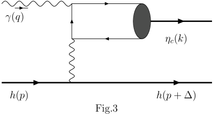
Figure 3: One of the two diagrams for photon exchange

The calculation of the $S$-matrix element is straightforward, we obtain:

$$\langle f|S|i\rangle_{em} = i2(eQ_{c})^{2}(2\pi)^{4}\delta^{4}(q-\Delta-k)\frac{1}{\sqrt{v^{0}}}\langle\eta_{c}|\psi^{\dagger}\chi|0\rangle\varepsilon_{\mu\nu\sigma\rho}\varepsilon^{\nu}\Delta^{\sigma}v^{\rho}$$ (56)

$$\cdot\frac{1}{\Delta^{2}+2m_{c}v\cdot\Delta}\cdot\frac{1}{\Delta^{2}}\cdot\langle h(p+\Delta)|J^{\mu}(0)|h(p)\rangle,$$

where $J^{\mu}$ is the operator of electric current, $Q_{c}$ is the charge fraction of $c$-quark in unit $e$. For $t\rightarrow-|t|_{min}$, one may use the method developed here to define a wave function for the $c$- or $\bar{c}$ quark propagating in a background field of soft photon to calculate the $S$-matrix element, the same result can be obtained if one neglects $\Delta^{2}$ in comparison to $2m_{c}v\cdot\Delta$ in the above equation. In this way one can also show that the contribution from a photon exchange combined with exchanging soft gluons is suppressed by $\Lambda^{2}/m_{c}^{2}$. For $h$ being a proton, the matrix element is decomposed with Dirac- and Pauli form factor:

$$\langle h(p+\Delta)|J^{\mu}(0)|h(p)\rangle=\bar{u}(p+\Delta)\left\{\gamma^{\mu}F_{1}(\Delta^{2})+i\sigma^{\mu\nu}\Delta_{\nu}\frac{F_{2}(\Delta^{2})}{2m}\right\}u(p),$$ (57)

for $t=-|t|_{min}$ the differential cross-section can be obtained directly. The dominant contribution reads:

$$\frac{d\sigma}{dt}|_{t=-|t|_{min}} \approx \frac{\alpha_{em}^{2}Q_{c}^{4}}{8m_{c}^{4}}\cdot\frac{|\langle\eta_{c}|\psi^{\dagger}\chi|0\rangle|^{2}}{m_{c}^{3}}\cdot\frac{s}{m^{2}}\cdot F_{1}^{2}(-|t|_{min})$$ (58)

$$\approx \frac{\alpha_{em}}{4m_{c}^{5}}\cdot\Gamma(\eta_{c}\rightarrow\gamma\gamma)\cdot\frac{s}{m^{2}},$$

where we use $F_{1}\approx e$ for the small momentum transfer. For large $t$, because the form factor $F_{1}(t)$ falls like $t^{-2}$[27] and the form factor $F_{2}(t)$ falls like $t^{-3}$[28], the differential cross-section will fall like $t^{-8}$. A model calculation in [9] for gluon exchange predicts that the differential cross-section falls $t^{-2}$. Hence, at large $t$ the differential cross-section with the photon exchange is highly suppressed. Because the detailed information of these form factors are not available, numerical result of this contribution to the total cross-section can not predicted. For small $t$, the differential cross-section increases as $1/t$, at $t=-|t|_{min}$ it increases with $s$ linearly, this is because the exchange photon becomes soft and its invariant mass decreases with $s^{-1}$. From Eq.(58) the differential cross-section in the forward region can be large, although it is suppressed by $\alpha_{em}^{3}$. The numerical value of $d\sigma/dt$ can be worked out, we have:

$$\frac{d\sigma}{dt}_{t=-|t|_{min}}\approx 8.4\times 10^{-4}\left(\frac{\sqrt{s}}{1{\rm GeV}}\right)^{2}\frac{{\rm nb}}{\rm GeV^{2}}.$$ (59)

where we used $m_{c}=1.5$GeV. With this estimation one can see that at $\sqrt{s}=100$GeV, the contribution from photon exchange is already at the same order as the estimation given in Eq.(54). It is also larger than the numerical values given in [9, 10, 11]. Hence, if the production of $\eta_{c}$ is observed in the extremely forward region the contribution from photon exchange is dominant for the production at energies relevant to HERA. This brings the difficulty to identify the effect due to Odderon exchange in the extremely forward region. For $s$ larger than those at HERA the contribution will still be dominant, if the contribution from Odderon exchange increases with $s$ as $s^{\alpha}$ for $\alpha<1$. Since the contribution from photon exchange decreases with increasing $|t|$ more rapidly than that of Odderon exchange, it is possible to identify the effect of Odderon exchange for suitable $|t|$ which is not very close to $|t|_{min}$. It requires a detailed study to identify kinematical regions for hunting Odderon.

7. Summary

In this work we have studied diffractive photoproduction of $\eta_{c}$. Taking charm quark as a heavy quark, the nonpertubative effect related to $\eta_{c}$ is represented by a NRQCD matrix element and $\eta_{c}$ can be taken as a bound state of $c\bar{c}$ quark. Then the production can be imagined as that the initial photon splits into a $c\bar{c}$ pair, this pair forms the $\eta_{c}$ after exchange of soft gluons with the initial hadron in the forward region. The problem of exchange of soft gluons can be studied with HQET and a systematic expansion in $m_{c}^{-1}$ can be employed. We find that the $S$-matrix element can be expressed in terms of wave-functions of $c$- and $\bar{c}$ quark, which propagates under a background field of gluons. The background field is dominated by components with long-wave lengthes corresponding to that the exchanged gluons are soft. By solving these wave functions with the expansion in $m_{c}^{-1}$, we can express the result for the $S$-matrix element with quantities, which are well defined in QCD. The $S$-matrix element in the forward region is expressed in the case of proton with four functions, which are defined with a twist-3 operator of gluons. If one thinks that the exchange of Odderon is responsible for the production, then the effect of Odderon is represented by these functions. For completeness, we also derive the $S$-matrix element for diffractive photoproduction of $J/\Psi$, the result is exactly the same as that derived in [18] with an assumption.

Since these four functions are unknown, numerical predictions can not be made in this work. However, an estimation in order of magnitude can be given in comparison with the production of $J/\Psi$. The estimation indicates that the differential cross-section of $\eta_{c}$ in the forward region is really small, in qualitative agreement with previous studies[9, 10, 11], where some models are used to make numerical predictions. However, from our results the differential cross-section of $\eta_{c}$ is not zero in the limit $t\rightarrow 0$, this is different than those predicted in [9, 10, 11]. The reason for this nonzero is that the initial hadron can change its helicity in this limit.

Instead of exchanging many soft gluons, a photon exchange can also contributes to the production of $\eta_{c}$. In the forward direction, i.e., $t\rightarrow 0$, one may find that this contribution is divergent. But, we should note that $t$ can approach to $0$ for $s\rightarrow\infty$, for large and finite $s$, the minimum value of $|t|$ is never zero because all particle in the final state are with finite masses. This minimum value makes the contribution finite. At this minimum value of $|t|$ the differential cross-section due to photon exchange can be predicted. We find that this contribution is large and is dominant for production of $\eta_{c}$. Hence, if $\eta_{c}$ is produced in the extremely forward region in experiment, one can not conclude that the $\eta_{c}$ is produced through Odderon exchange and the effect of Odderon is observed. At large $|t|$, it can be shown that the differential cross-section with the photon exchange falls like $t^{-8}$ and can be neglected. Therefore, if $\eta_{c}$ is produced with $|t|$ which is not very close to its minimal value, one can identify the production as an effect of Odderon to confirm the existence of Odderon in this process.

Our results for scattering amplitudes are expressed with quantities like NRQCD matrix element and matrix element of the twist-3 operator of gluons, they are well defined in the framework of QCD and are universal, i.e., they do not depend on specific processes. Nonperturbative methods like lattice QCD or sum rule method may be used to determine them. The matrix element of the twist-3 operator is unfortunately unknown at the moment, this fact prevents us to make numerical predictions. But, with our results one can build more realistic models to have a reliable prediction for diffractive photoproduction of $\eta_{c}$.

Acknowledgments

The author would like to thank Prof. O. Nachtmann and Prof. J.S. Xu for interesting discussions. He would also like to thank Prof. X.D. Ji for reading the manuscript and comments. This work is supported by National Nature Science Foundation of P. R. China with the grand No. 19925520.

References

• [1] L.Lukaszuk and B. Nicolescu, Lett. Nuovo Cim. 8 (1973) 405.
• [2] M.A. Braun, ”Odderon and QCD”, hep-ph/9805394.
• [3] A. Breakstone et al., Phys. Rev. Lett. 54 (1985) 2180. S. Erhan et al., Phys. Lett. B152 (1985) 131.
• [4] H.G. Dosch, C. Ewerz and V. Schatz, Eur. Phys. J. C24 (2002) 561.
• [5] A. SchΓ€fer, L. Mankiewicz, and O. Nachtmann: Diffractive $\eta_{c},\eta,\eta^{\prime},J/\psi$ and $\psi^{\prime}$ production in electron-proton collisions at HERA energies in: Proceedings of the Workshop Physics at HERA, 1991 (W. BuchmΓΌller and G. Ingelman, eds.), DESY, Hamburg (1992).
• [6] W. Kilian, O. Nachtmann, Eur. Phys. J. C 5, 317 (1998).
• [7] E.R. Berger, A. Donnachie, H.G. Dosch, W. Kilian, O. Nachtmann and M. Rueter, Eur.Phys.J. C9 (1999) 491, E.R. Berger, A. Donnachie, H.G. Dosch, O. Nachtmann, Eur.Phys.J. C14 (2000) 673.
• [8] P. Hagler, B. Pire, L. Szymanowski and O.V. Teryaev, Eur.Phys.J.C26:261-270,2002.
• [9] J. Czy$\dot{\rm z}$ewski, J. KwieciΕ„ski, L. Motyka, and M. Sazikowski: Phys. Lett. B 398 (1997) 400, Erratum: ibid B 411, 402 (1997).
• [10] R. Engel, D. Y. Ivanov, R. Kirschner, and L. Szymanowski: Eur. Phys. J. C 4, 93 (1998).
• [11] J. Bartels, M.A. Braun, D. Colferai and G.P. Vacca, Eur.Phys.J. C20 (2001) 323.
• [12] C. Adloff et al., H1 Collaboration Phys.Lett. B544 (2002) 35.
• [13] N. Isgur and M.B. Wise, Phys. Lett. B232 (1989) 113, ibid. B237 (1990) 527, E. Eichten and B. Hill, Phys. Lett. B234 (1990) 511, B. Grinstein, Nucl. Phys. B339 (1990) 253, H. Georgi, Phys. Lett. B240 (1990) 447.
• [14] G.T. Bodwin, E. Braaten, and G.P. Lepage, Phys. Rev. D51, 1125 (1995); Erratum:ibid., D55, 5853 (1997).
• [15] O. Nachtmann, Ann. Phys. Vol. 209 (1991) 436.
• [16] J.P. Ma, Nucl. Phys. B602 (2001) 572.
• [17] J.P. Ma and J.S. Xu, Eur.Phys.J. C24 (2002) 261.
• [18] J.P. Ma and J.S.Xu, Nucl.Phys. B640 (2002) 283.
• [19] M.E. Peskin, Nucl. Phys. B156 (1979) 365, G. Bhanot and M.E. Peskin, Nucl. Phys. B156 (1979) 391, T.M. Yan, Phys. Rev. D22 (1980) 1652 Y.P. Kuang and T.M. Yan, Phys.Rev.D24:2874,1981
• [20] M.G. Ryskin, Z. Phys. C57 (1993) 89, M.G. Ryskin et al., ibid., C76 (1997) 231, L.L. Frankfurt, W. Koepf and M. Strikman, Phys. Rev. D57 (1998) 512, ibid., D54 (1996) 3194, L. Frankfurt, M. McDermott and M. Strikman, JHEP 0103 (2001) 045,
• [21] M. Diehl, Eur.Phys.J. C19 (2001) 485.
• [22] P.Hoodbhoy and X. Ji, Phys. Rev. D58 (1998) 054006.
• [23] X.D. Ji, J.P. Ma and F.Yuan, Nucl. Phys. B652 (2003) 383.
• [24] X.D. Ji, Phys. Rev. Lett. 78 (1997) 610, Phys. Rev. D55 (1997) 7114, J.Phys. G24 (1998) 1181.
• [25] J. Bartels, Nucl. Phys. B 175 (1980) 365; J. Kwiecinski and M. Praszalowicz, Phys. Lett. B 94 (1980) 413.
• [26] H1 Collaboration, C. Adloff et al., Phys. Lett. B483 (2000) 23; S. Aid et al., Nucl. Phys. B472 (1996) 3, ZEUS Collaboration, J. Breitweg et al., Z. Phys. C75 (1997) 215; M. Derrick et al., Phys. Lett. B350 (1995) 120.
• [27] G.P. Lepage and S.J. Brodsky, Phys. Rev. D22 (1980) 2157.
• [28] A.V. Belitsky, X.D. Ji and F. Yuan, hep-ph/0212351.