What can we learn from $B^{+}\to D^{(*)-}_{s}K^{+}\pi^{+}$, $B_{d}\to D_{s}^{(*)-}K^{0}\pi^{+}$ and $B_{d}\to D_{s}^{(*)-}K^{*+}$ decays?

Abstract

We study the nonresonant three-body decays of $B^{+}\to D^{(*)-}_{s}K^{+}\pi^{+}$ and $B_{d}\to D_{s}^{(*)-}K^{0}\pi^{+}$. We find that these decays can provide the information on the time-like form factors of $D^{(*)}_{s}K$. We also explicitly investigate $B_{d}\to D_{s}^{(*)-}K^{*+}$ decays by discriminating the nonresonant contributions with the unknown $D^{(*)}_{s}$ wave functions being fixed by the measured mode of $B_{d}\to D_{s}^{-}K^{+}$.

Three-body decays of $B$ meson have recently been noticed in the experiments by the analyses of the Dalitz plots and invariant mass distributions Belle-PRD . The study of the three-body decays provides not only the method to extract the CP violating phase angles CP , but also the way to understand or search the uncertain particle states, such as $f_{0}(400-1200)$, $f_{0}(980)$, $a_{0}(980)$ Chen-PRD and glueballs CHT . Moreover, it also helps us to build up the QCD approach for the nonresonant three-body decays ChenLi . As known that the charmless three-body decays of $B$ meson are dominated by the so-called quasi-two-body decays CY , it is not easy to discriminate the nonresonant states from resonant ones. However, this may not be the case in those final states with charmed mesons.

It has been demonstrated by Belle Belle-PLB that $B_{d}\to D^{(*)-}\bar{K}^{0}K^{+}$ decays are actually dominated by the three-body modes because the $\bar{K}^{0}K^{+}$ system is confirmed to be an $J^{P}=1^{-}$ state by the analysis of angular dependence. The production of the decays can be thought easily by the consequence of $b\to c\bar{u}d$, while $\bar{K}^{0}K^{+}$ is produced by the created $s\bar{s}$ pair and $\bar{u}d$. Therefore, if annihilation topologies are neglected, the dominant topologies for the decays correspond to $B_{d}\to D^{(*)-}$ and a outgoing pair of $\bar{K}^{0}K^{+}$. The formers are described by $B_{d}\to D^{(*)-}$ form factors, calculated by some QCD approaches such as perturbative QCD (PQCD), quark model, QCD sum rules and light-cone QCD sum rules, while the latters respond the times-like form factors which can be fixed via the connection to electromagnetic form factors and fitting with experiments Balakin . Although time-like form factors of $KK$, denoted by $F^{0\to KK}$, are not easy to be formulated in theory, $B_{d}\to D^{(*)-}\bar{K}^{0}K^{+}$ is a good candidate to study the nonresonant three-body decays. According to the observations of Belle, we know that the branching ratios (BRs) of $B_{d}\to D^{(*)-}\bar{K}^{0}K^{+}$ decays are of ${\cal O}(10^{-4})$. It means that the effects of $F^{0\to KK}$ are not small. Moreover, following the analysis of Ref. CHST , we see that the peaks in the $KK$ spectra of the decays locate at around $1.5$ GeV. This can be understood that the region is actually governed by PQCD where the proper hard scale is around $\sqrt{\bar{\Lambda}m_{B}}$ ChenLi with $\bar{\Lambda}=m_{B}-m_{b}$. By taking $\bar{\Lambda}\approx 0.48$ and $m_{B}=5.28$ GeV, the value of $\sqrt{\bar{\Lambda}m_{B}}$ is $1.6$ GeV, quite close to the consequence of Ref. CHST . In some senses, PQCD approach can deal with the three-body decays by combing with the experimental fittings of time-like form factors.

Inspired by the large BRs of $B_{d}\to D^{(*)-}\bar{K}^{0}K^{+}$ decays, one can speculate that the three-body decay related to form factors $\langle DP|V_{\mu}-A_{\mu}|B\rangle$ can be also large, saying ${\cal O}(10^{-5}-10^{-4})$, where $D(P)$ is the charmed (pseudoscalar) meson and $V_{\mu}(A_{\mu})$ is the vector (axial-vector) current. In theoretical viewpoints, the question is hard to answer since there are too much unknown form factors involved and no direct experimental data related to them. However, we still can give some conjectures on the relevant decays. Firstly, in terms of the concept of two-meson wave functions MP , the $DP$ system could be described by a set of wave functions for $\langle DP|V_{\mu}-A_{\mu}|B\rangle$ and they can be related to the time-like form factors of $DP$, denoted by $F^{0\to DP}$. Therefore, if the $K$ meson is massless particle, the threshold invariant mass, expressed by $\omega$, to generate the $KK$ pair is about $0$. However, unlike the case of the $KK$ pair production, since charmed meson is a massive particle, to produce the $DP$ pair it should start from $m_{D}$. By assuming that the peak of the $DP$ pair spectrum is around $m_{D}+\sqrt{\bar{\Lambda}m_{B}}$, we can expect that the BR associated with $F^{0\to DP}$ form factors should be smaller than that associated with $F^{0\to KK}$ because the dominant form factors have been shifted to a larger $\omega$ region and their values are small, compared to $F^{0\to KK}$ at $\sqrt{\bar{\Lambda}m_{B}}$. Moreover, if the third particle of the involving three-body decay is a light meson, although the allowed $\omega$ of $DP$ could reach the value of $m_{B}$ ( it is $m_{B}-m_{D}$ in the $B_{d}\to D^{(*)-}\bar{K}^{0}K^{+}$ decays), due to the suppression of phase space factor $(1-\omega^{2}/m^{2}_{B})$, the effects of the large $\omega$ are not important. Therefore, the available phase space is smaller than that in the decays of $B_{d}\to D^{(*)-}\bar{K}^{0}K^{+}$. Hence we conjecture that the BR of $B\to DPP^{\prime}$ should be smaller than those of $B_{d}\to D^{(*)-}\bar{K}^{0}K^{+}$ decays, where $DP$ system and $B$ meson have the same light spectator. Note that the chosen examples have the same weak Wilson coefficients (WCs).

Because there is no any direct information on $F^{0\to DP}$, in order to confirm our conjectures, we suggest that the observations of $B^{+}\to D^{(*)-}_{s}K^{+}\pi^{+}$ and $B_{d}\to D^{(*)-}_{s}K^{0}\pi^{+}$, illustrated by Fig. 1, can help us to find the answer. Since the former modes correspond to pure three-body decays and once they are measured in experiments, we immediately know what the effects of $F^{0\to DP}$ are. However, besides the nonresonant three-body decays, the decays of $B_{d}\to D^{(*)-}_{s}K^{0}\pi^{+}$ also involve resonant states $B_{d}\to D^{(*)-}_{s}K^{*+}(K^{*+}\to K^{0}\pi^{+})$. Recently, Belle Belle and Babar Babar have measured the relevant two-body decay $B_{d}\to D^{-}_{s}K^{+}$ to be $(4.6^{+1.2}_{-1.1}\pm 1.3)\times 10^{-5}$ and $(3.2\pm 1.0\pm 1.0)\times 10^{-5}$, respectively. One expects that the $B_{d}\to D^{(*)-}_{s}K^{*+}$ decays should have the same magnitudes in BR. Probably, the suggested three-body decays also have the same BRs in order of magnitudes. In order to understand more on the nonresonant parts in $B_{d}\to D^{(*)-}_{s}K^{0}\pi^{+}$, it is important to know how large the contributions are from quasi-two-body decays. In this paper, we want to make a detailed analysis on $B_{d}\to D^{(*)-}_{s}K^{*+}$ decays.

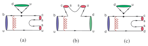
Figure 1: The topologies for the nonresonant three-body decays (a, b) $B^{+}\to D^{(*)-}_{s}K^{+}\pi^{+}$ and (c) $B_{d}\to D^{(*)-}_{s}K^{0}\pi^{+}$. The dots denote the weak vertices.

Since the considered decays correspond to the $b\to c\bar{d}u$ transition, we describe the effective Hamiltonian as

$$H_{{\rm eff}} = \frac{G_{F}}{\sqrt{2}}\sum_{q=u,c}V_{q}\left[C_{1}(\mu){\cal O}_{1}^{(q)}+C_{2}(\mu){\cal O}_{2}^{(q)}\right]$$

$${\cal O}_{1}^{(q)} = \bar{d}_{\alpha}q_{\beta}\bar{c}_{\beta}b_{\alpha}\,,\ \ \ {\cal O}_{2}^{(q)}\;=\;\bar{d}_{\alpha}q_{\alpha}\bar{c}_{\beta}b_{\beta}$$ (1)

where $\bar{q}_{\alpha}q_{\beta}=\bar{q}_{\alpha}\gamma_{\mu}(1-\gamma_{5})q_{\beta}$, $\alpha(\beta)$ are the color indices, $V_{q}=V_{qd}^{*}V_{cb}$ are the products of the CKM matrix elements CKM , and $C_{1,2}(\mu)$ are the WCs BBL . Conventionally, the effective WCs of $a_{2}=C_{1}+C_{2}/N_{c}$ and $a_{1}=C_{2}+C_{1}/N_{c}$ with $N_{c}=3$ being color number are more useful. It is known that the difficulty for studying exclusive hadron decays is from the calculations of matrix elements. In order to handle the hadronic effects, we employ the PQCD approach in which the transition matrix element is described by the convolution of hadron wave functions and the hard amplitude of the valence quarks LB ; Li . Although the PQCD approach suffers singularities from end-point region, they could be smeared after the threshold and the $k_{T}$ resummation effects are included. The latter arises from the introduction of the parton transverse momentum KLS-PRD ; CKL-PRD . In the literature, the applications of PQCD to exclusive $B$ meson decays, such as $B\rightarrow K\pi$ KLS , $B\rightarrow\pi\pi(KK)$ LUY ; CL-PRD ; Chen-PLB520 , $B\rightarrow\phi\pi(K)$ Melic ; CKL-PRD , $B\rightarrow\eta^{(^{\prime})}K$ KS , $B\rightarrow\rho K$ Chen-PLB525 decays and $B\to K^{(*)}\ell^{+}\ell^{-}$ CQ-PRD , have been studied and found that all of them are consistent with the current experimental data SU ; Keum . We think that the same approach can be also used to the considered cases here.

It has been shown that by the reality of hierarchy $m_{B}>>m_{D^{(*)}_{s}}>>\bar{\Lambda}$, the distribution amplitudes of $B(D^{(*)}_{s})$ mesons can be described by Li-P

$$\langle 0|\bar{b}(0)_{j}d(z)_{l}|B,p_{1}\rangle = \frac{1}{\sqrt{2N_{c}}}\int^{1}_{0}dxe^{-ixp_{1}\cdot z}\Big{\{}[/p_{1}+m_{B}]_{lj}\gamma_{5}\Phi_{B}(x)\Big{\}},$$ (2)

$$\langle D_{s},p_{2}|\bar{d}(0)_{j}c(z)_{l}|0\rangle = \frac{1}{\sqrt{2N_{c}}}\int^{1}_{0}dxe^{ixp_{2}\cdot z}\Big{\{}\gamma_{5}[/p_{2}+m_{D_{s}}]_{lj}\Phi_{D_{s}}(x)\Big{\}},$$

$$\langle D^{*}_{s},p_{2}|\bar{d}(0)_{j}c(z)_{l}|0\rangle = \frac{1}{\sqrt{2N_{c}}}\int^{1}_{0}dxe^{ixp_{2}\cdot z}\Big{\{}/\varepsilon_{2}[/p_{2}+m_{D^{*}_{s}}]_{lj}\Phi_{D^{*}_{s}}(x)\Big{\}},$$ (3)

where $\varepsilon_{2\mu}$ is the polarization vector of $D^{*}_{s}$ meson, the normalizations of wave functions are taken to be $\int^{1}_{0}dx\Phi_{B(D^{(*)}_{s})}(x)=f_{B(D^{(*)}_{s})}/2\sqrt{2N_{c}}$ and $f_{B(D^{(*)}_{s})}$ are the corresponding decay constants. Although the decay constants and wave functions of $D^{*}_{s}$ between longitudinal and transverse polarizations are different generally, for simplicity, we assume that they are the same. Since the effects of transverse polarization parts are always related to the factor $r_{2}=m_{D^{*}_{s}}/M_{B}$, one expects that their contributions are much smaller than those from longitudinal parts. As to the distribution amplitude of the $K^{*}$ meson, we refer to the results derived from QCD sum rules BBKT and summarize them as

$$\langle 0|\bar{u}(0)_{j}s(z)_{l}|K^{*},p_{3}\rangle = \frac{1}{\sqrt{2N_{c}}}\int^{1}_{0}dxe^{-ixp_{3}\cdot z}\Big{[}m_{K^{*}}[/\varepsilon_{3L}]_{lj}\Phi_{K^{*}}(x)+[/\varepsilon_{3L}/p_{3}]_{lj}\Phi_{K^{*}}^{t}(x)$$ (4)

$$+m_{K^{*}}[I]_{lj}\Phi_{K^{*}}^{s}(x)+m_{K^{*}}[/\varepsilon_{3T}]_{lj}\Phi_{K^{*}}^{v}(x)$$

$$+[/\varepsilon_{3T}/p_{3}]_{lj}\Phi_{K^{*}}^{T}(x)+m_{K^{*}}[/{\cal C}]_{lj}\Phi_{K^{*}}^{a}(x)\Big{]},$$

where $\varepsilon_{3L(T)}$ denote the longitudinal (transverse) polarization vectors of $K^{*}$ meson, ${\cal C}_{\mu}=$ $i\epsilon_{\mu\nu\rho\sigma}$ $\varepsilon_{3T}^{\nu}p_{3}^{\rho}n_{-}^{\sigma}/{p_{3}\cdot n_{-}}$ in which $n_{-}$ is parallel to the large component of $p_{3}$, and $\Phi_{K^{*}}^{(T)}$ correspond to twist-2 wave functions while the remains stand for the twist-3 ones. In addition, in terms of light-cone coordinate, the momenta of various mesons and the light valence quarks inside the corresponding mesons are assigned as: $p_{1}=m_{B}/\sqrt{2}(1,1,\vec{0}_{T})$, $k_{1}=m_{B}/\sqrt{2}(x_{1},0,\vec{k}_{1T})$; $p_{2}=m_{B}/\sqrt{2}(1,r^{2}_{2},\vec{0}_{T})$, $k_{2}=m_{B}/\sqrt{2}(x_{2},0,\vec{k}_{2T})$; $p_{3}=m_{B}/\sqrt{2}(0,1-r^{2}_{2},\vec{0}_{T})$, $k_{3}=m_{B}/\sqrt{2}(0,(1-r^{2}_{2})x_{3},\vec{k}_{3T})$.

As usual, we have the decay rate for $B_{d}\to D^{-}_{s}K^{*+}$ decay as

$$\Gamma=\frac{G^{2}P_{c}m^{2}_{B}}{16\pi}|A_{D_{s}^{-}K^{*+}}|^{2},$$

where $P_{c}\equiv|p_{2z}|=|p_{3z}|$ and the amplitude of $A_{D_{s}^{-}K^{*+}}$ is given by

$$A_{D_{s}^{-}K^{*+}}=f_{B}F_{D_{s}^{-}K^{*+}}+M_{D_{s}^{-}K^{*+}}.$$ (5)

The first (second) term in Eq. (5) comes from the factorizable (nonfactorizable) contributions, illustrated by Fig. 2a (2b).

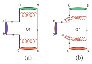
Figure 2: The topologies (a) factorizable (b) nonfactorizable effects for the decays $B_{d}\to D^{(*)-}_{s}K^{*+}$.

The hard amplitudes $F_{D_{s}^{-}K^{*+}}$ and $M_{D_{s}^{-}K^{*+}}$ are expressed by

$$F_{D_{s}^{-}K^{*+}} = -8\pi C_{F}m^{2}_{B}\int_{0}^{1}d[x]\int_{0}^{\infty}[b]d[b]\Phi_{D_{s}}(x_{2})$$ (6)

$$\Big{\{}\Big{[}(r^{2}_{2}-(1-2r^{2}_{2})x_{3})\Phi_{K^{*}}(\zeta)+r_{2}r_{3}\Big{(}(1-2x_{3})\Phi^{t}_{K^{*}}(\zeta)+(1+2x_{3})\Phi^{s}_{K^{*}}(\zeta)\Big{)}\Big{]}$$

$$\times{\cal E}_{a}^{1}(t^{1}_{a})+\Big{[}(1-r^{2}_{2})x_{2}\Phi_{K^{*}}(\zeta)-r_{2}r_{3}(1+x_{2})\Phi^{s}_{K^{*}}(\zeta)\Big{]}{\cal E}_{a}^{2}(t^{2}_{a})\Big{\}},$$

$$M_{D_{s}^{-}K^{*+}} = 16\pi C_{F}m_{B}^{2}\sqrt{2N_{c}}\int_{0}^{1}d[x]\int_{0}^{\infty}[b]d[b]\Phi_{B}(x_{1},b_{1})\Phi_{D_{s}}(x_{2})$$ (7)

$$\Big{\{}\Big{[}-(r_{2}^{2}x_{2}+(1-2r_{2}^{2})x_{3})\Phi_{K^{*}}(\zeta)+r_{2}r_{3}\Big{(}(x_{2}-x_{3})\Phi^{t}_{K^{*}}(\zeta)$$

$$+(x_{2}+x_{3})\Phi^{s}_{K^{*}}(\zeta)\Big{)}\Big{]}{\cal E}_{f}^{1}(t^{1}_{f})+\Big{[}(x_{2}-r^{2}_{2})\Phi_{K^{*}}(\zeta)$$

$$-r_{2}r_{3}\Big{(}(x_{3}-x_{2})\Phi_{K^{*}}^{t}(\zeta)+(2+x_{2}+x_{3})\Phi_{K^{*}}^{s}(\zeta)\Big{)}\Big{]}{\cal E}_{f}^{2}(t^{2}_{f})\Big{\}},$$

with $r_{3}=m_{K^{*}}/m_{B}$ and $\zeta=1-x_{3}$. In our considerations, the small effects from $r^{2}_{3}\approx 0.028$ and $r^{3}_{2}\approx 0.05$ are neglected. The evolution factors ${\cal E}_{a(f)}^{i}$ are defined by

$${\cal E}^{i}_{a}(t^{i}_{a}) = \Big{(}C_{1}(t^{i}_{a})+\frac{C_{2}(t^{i}_{a})}{N_{c}}\Big{)}\alpha_{s}(t^{i}_{a})S_{K^{*}+D_{s}}(t^{i}_{a})h_{a}(\{x\},\{b\}),$$

$${\cal E}^{i}_{f}(t^{i}_{f}) = \frac{C_{2}(t^{i}_{f})}{N_{c}}\alpha_{s}(t^{i}_{f})S_{B+D_{s}+K^{*}}(t^{i}_{f})h^{i}_{f}(\{x\},\{b\}),$$

where $t^{1,2}_{a,f}$ denote the hard scales and are chosen as

$$t^{1}_{a} = max(m_{B}\sqrt{(1-r^{2}_{2})x_{3}},\frac{1}{b_{2}},\frac{1}{b_{3}}),\ \ \ t^{2}_{a}=max(m_{B}\sqrt{(1-r^{2}_{2})x_{2}},\frac{1}{b_{2}},\frac{1}{b_{3}}),$$

$$t^{j}_{f} = max(m_{B}\sqrt{F^{2}_{j}},m_{B}\sqrt{(1-r^{2}_{2})x_{2}x_{3}},\frac{1}{b_{2}},\frac{1}{b_{3}}),$$

$$F^{2}_{1} = (1-r^{2}_{2})(x_{1}-x_{2})x_{3},\ \ \ F^{2}_{2}=x_{1}+x_{2}+(1-r^{2}_{2})(1-x_{1}-x_{2})x_{3}.$$ (8)

Here, $S_{K^{*}+D_{s}}=S_{K^{*}}(k^{-}_{3},p^{-}_{3}-k_{3}^{-})S_{D_{s}}(k^{+}_{2})$ and $S_{B+D_{s}+K^{*}}=S_{B}(k^{+}_{1})S_{D_{s}}(k^{+}_{2})S_{K^{*}}(k^{-}_{3},p^{-}_{3}-k_{3}^{-})$ are the associated Sudakov factors. We note that only the light valence quarks of $B$ and $D^{(*)}_{s}$ mesons have the Sudakov effects Li . $h_{a,f}$ describe the hard functions arising from the propagators of gluon and internal valence quark. Their detailed expressions with threshold resummation effects can be found in Ref. CKL-PRD .

It is known that besides the longitudinal polarization, there also involve two transverse polarizations in $B\to VV$ decays CKL-PRD2 , where $V$ denotes the vector meson. Therefore, the $B_{d}\to D_{s}^{*-}K^{*+}$ decay amplitude will be more complicated than those in $B\to VP$ or $PP$ decays with $P$ being the pseudoscalar meson. In terms of helicity basis, the $B_{d}\to D^{*-}_{s}K^{*+}$ decay rate is written as

$$\Gamma=\frac{G_{F}^{2}P_{c}}{16\pi m^{2}_{B}}\sum_{h=L,T}{\cal M}^{(h)\dagger}{\cal M}^{(h)},$$

where the superscript $h$ denotes the helicity states of the two vector mesons. The amplitude ${\cal M}^{(h)}$ is decomposed into

$${\cal M}^{(h)} = \epsilon_{2h\mu}^{*}\epsilon_{3h\nu}^{*}\left[a\,\,g^{\mu\nu}+{b\over m_{D^{*}_{s}}m_{K^{*}}}p_{1}^{\mu}p_{1}^{\nu}+i{c\over m_{D^{*}_{s}}m_{K^{*}}}\epsilon^{\mu\nu\alpha\beta}p_{2\alpha}p_{3\beta}\right],$$ (9)

$$\equiv m_{B}^{2}{\cal M}_{L}+m_{B}^{2}{\cal M}_{N}\epsilon^{*}_{2T}\cdot\epsilon^{*}_{3T}+i{\cal M}_{T}\epsilon^{\alpha\beta\gamma\rho}\epsilon^{*}_{2T\alpha}\epsilon^{*}_{3T\beta}p_{2\gamma}p_{3\rho}\,,$$

with the convention of $tr(\gamma_{5}\not a\not b\not c\not d)=-4i\epsilon^{\alpha\beta\gamma\rho}a_{\alpha}b_{\beta}c_{\gamma}d_{\rho}$ and the definitions of

$$m_{B}^{2}{\cal M}_{L} = a\,\,\epsilon_{2L}^{*}\cdot\epsilon_{3L}^{*}+{b\over m_{D^{*}_{s}}m_{K^{*}}}\epsilon_{2L}^{*}\cdot p_{1}\,\epsilon_{3L}^{*}\cdot p_{1},$$

$$m_{B}^{2}{\cal M}_{N} = a\,\,\epsilon_{2T}^{*}\cdot\epsilon_{3T}^{*},$$

$${\cal M}_{T} = {c\over m_{D^{*}_{s}}m_{K^{*}}}.$$ (10)

Similar to $B_{d}\to D_{s}K^{*+}$, the decay amplitudes corresponding to each polarizations can be written as

$${\cal M}_{L(N,T)} = f_{B}F_{L(N,T)}+M_{L(N,T)},$$

where the first (second) term expresses factorized (nonfactorized) effects. Each hard amplitudes can be formulated by

$$F_{L} = -8\pi C_{F}m_{B}^{2}\int_{0}^{1}d[x]\int_{0}^{\infty}bd[b]\Phi_{D^{*}}(x_{2})$$ (11)

$$\times\Big{\{}\left[(r^{2}_{2}+(1-r^{2}_{2})x_{3})\Phi_{K^{*}}(\zeta)+r_{2}r_{3}\left(\Phi^{t}_{K^{*}}(\zeta)-\Phi^{s}_{K^{*}}(\zeta)\right)\right]{\cal E}_{a}^{1}(t^{1}_{a})$$

$$-\left[(1-r^{2}_{2})x_{2}\Phi_{K^{*}}(\zeta)+2r_{2}r_{3}(1-x_{2})\Phi^{s}_{K^{*}}(\zeta)\right]{\cal E}_{a}^{2}(t^{2}_{a})\Big{\}},$$

$$F_{N} = -8\pi C_{F}m_{B}^{2}r_{2}r_{3}\int_{0}^{1}d[x]\int_{0}^{\infty}bd[b]\Phi_{D^{*}}^{T}(x_{2})$$ (12)

$$\times\Big{\{}\left[(1+x_{3})\Phi^{v}_{K^{*}}(\zeta)+\left(-\frac{r_{2}}{r_{3}}\Phi^{T}_{K^{*}}(\zeta)+(1-x_{3})\Phi^{a}_{K^{*}}(\zeta)\right)\right]{\cal E}_{a}^{1}(t^{1}_{a})$$

$$-\left[(1+x_{2})\Phi_{K^{*}}^{v}(\zeta)-(1-x_{2})\Phi^{a}_{K^{*}}(\zeta)\right]{\cal E}_{a}^{2}(t^{2}_{a})\Big{\}},$$

$$F_{T} = -16\pi C_{F}m_{B}^{2}r_{2}r_{3}\int_{0}^{1}d[x]\int_{0}^{\infty}bd[b]\Phi_{D^{*}}^{T}(x_{2})$$ (13)

$$\times\Big{\{}\left[(1-x_{3})\Phi^{v}_{K^{*}}(\zeta)+\left(\frac{r_{2}}{r_{3}}\Phi^{T}_{K^{*}}(\zeta)+(1+x_{3})\Phi^{a}_{K^{*}}(\zeta)\right)\right]{\cal E}_{a}^{1}(t^{1}_{a})$$

$$-\left[(1+x_{2})\Phi_{K^{*}}^{a}(\zeta)-(1-x_{2})\Phi^{v}_{K^{*}}(\zeta)\right]{\cal E}_{a}^{2}(t^{2}_{a})\Big{\}},$$

$$M_{L} = 16\pi C_{F}M_{B}^{2}\sqrt{2N_{c}}\int_{0}^{1}d[x]\int_{0}^{\infty}[b]d[b]\Phi_{B}(x_{1},b_{1})\Phi_{D^{*}}(x_{2})$$ (14)

$$\times\Big{\{}\Big{[}(1-2r^{2}_{2})x_{3}\Phi_{K^{*}}(\zeta)+r_{2}r_{3}\Big{(}(x_{3}+x_{2})\Phi^{t}_{K^{*}}(\zeta)+(x_{2}-x_{3})\Phi^{s}_{K^{*}}(\zeta)\Big{)}\Big{]}{\cal E}_{f}^{1}(t^{1}_{f})$$

$$+\Big{[}-(r^{2}_{2}+(1-2r^{2}_{2})x_{2})\Phi_{K^{*}}(\zeta)+r_{2}r_{3}\Big{(}(2-x_{2}-x_{3})\Phi^{t}_{K^{*}}(\zeta)$$

$$+(x_{2}-x_{3})\Phi^{s}_{K^{*}}(\zeta)\Big{)}\Big{]}{\cal E}_{f}^{2}(t^{2}_{f})\Big{\}},$$

$$M_{N} = -32\pi C_{F}m_{B}^{2}\sqrt{2N_{c}}r_{2}r_{3}\int_{0}^{1}d[x]\int_{0}^{\infty}[b]d[b]\Phi_{B}(x_{1},b_{1})\Phi_{D^{*}}(x_{2})\Phi^{v}_{K^{*}}(\zeta){\cal E}_{f}^{2}(t^{2}_{f}),$$ (15)

$$M_{T} = -64\pi C_{F}m_{B}^{2}\sqrt{2N_{c}}r_{2}r_{3}\int_{0}^{1}d[x]\int_{0}^{\infty}[b]d[b]\Phi_{B}(x_{1},b_{1})\Phi_{D^{*}}(x_{2})\Phi^{a}_{K^{*}}(\zeta){\cal E}_{f}^{2}(t^{2}_{f}).$$ (16)

From the above equations, we see clearly that the hard amplitudes for the transverse polarizations are proportional to factors of $r_{2}r_{3}$ and $r^{2}_{2}$. One of two $r_{2}$ in the latter comes from the mass of charm-quark $m_{c}$ that we already set $m_{c}\approx m_{D^{(*)}_{s}}$ due to $m_{D_{s}^{(*)}}-m_{c}\sim\bar{\Lambda}$.

To get numerical estimations, we model the $B$-meson wave function $\Phi_{B}$ to be

$$\Phi_{B}(x,b) = N_{B}x^{2}(1-x)^{2}\exp\Big{[}-\frac{1}{2}\Big{(}\frac{x\,m_{B}}{\omega_{B}}\Big{)}^{2}-\frac{\omega_{B}^{2}b^{2}}{2}\Big{]}$$ (17)

where $b$ is the conjugate variable of the transverse momentum of the light quark, $N_{B}$ can be determined by the normalization of the wave function at $b=0$ and $\omega_{B}$ is the shape parameter. Since the wave functions of the $K^{*}$ meson are derived in the framework of QCD sum rules, we express them up to twist-3 directly by BBKT

$$\Phi_{K^{*}}(x) = \frac{3f_{K^{*}}}{\sqrt{2N_{c}}}x(1-x)\Big{[}1+0.57(1-2x)+0.07C^{3/2}_{2}(1-2x)\Big{]}\;,$$

$$\Phi_{K^{*}}^{t}(x) = \frac{f_{K^{*}}^{T}}{2\sqrt{2N_{c}}}\bigg{\{}0.3(1-2x)\left[3(1-2x)^{2}+10(1-2x)-1\right]+1.68C^{1/2}_{4}(1-2x)$$

$$+0.06(1-2x)^{2}\left[5(1-2x)^{2}-3\right]+0.36\left[1-2(1-2x)(1+\ln(1-x))\right]\bigg{\}}\;,$$

$$\Phi_{K^{*}}^{s}(x) = \frac{f_{K^{*}}^{T}}{2\sqrt{2N_{c}}}\bigg{\{}3(1-2x)\left[1+0.2(1-2x)+0.6(10x^{2}-10x+1)\right]$$

$$-0.12x(1-x)+0.36[1-6x-2\ln(1-x)]\bigg{\}}\;,$$

$$\Phi_{K^{*}}^{T}(x) = \frac{3f_{K^{*}}^{T}}{\sqrt{2N_{c}}}x(1-x)\Big{[}1+0.6(1-2x)+0.04C^{3/2}_{2}(1-2x)\Big{]}\;,$$

$$\Phi_{K^{*}}^{v}(x) = \frac{f_{K^{*}}}{2\sqrt{2N_{c}}}\bigg{\{}\frac{3}{4}\Big{[}1+(1-2x)^{2}+0.44(1-2x)^{3}\Big{]}+0.4C^{1/2}_{2}(1-2x)$$

$$+0.88C^{1/2}_{4}(1-2x)+0.48[2x+\ln(1-x)]\bigg{\}}\;,$$

$$\Phi_{K^{*}}^{a}(x) = \frac{f_{K^{*}}}{4\sqrt{2N_{c}}}\Big{\{}3(1-2x)\Big{[}1+0.19(1-2x)+0.81(10x^{2}-10x+1)\Big{]}$$

$$-1.14x(1-x)+0.48[1-6x-2\ln(1-x)]\Big{\}}\;,$$

with the Gegenbauer polynomials,

$$C_{2}^{1/2}(\xi)=\frac{1}{2}(3\xi^{2}-1)\;,\;\;\;\;C_{4}^{1/2}(\xi)=\frac{1}{8}(35\xi^{4}-30\xi^{2}+3)\;,\;\;\;\;C_{2}^{3/2}(\xi)=\frac{3}{2}(5\xi^{2}-1)\;.$$

Although there are theoretical errors on the coefficients of the wave functions, we find that the allowed errors in these derived wave functions change the BRs only at a few percent level so that we will not discuss them further. In the PQCD approach, the wave functions represent the nonperturbative QCD effects and have the universal property. In principle, they can be determined by some specific measured modes. Hence, the unknown $\omega_{B}$ can be fixed by such as $B\to\phi K$ decays, in which $\phi$ and $K$ meson wave functions have been determined in the literature. Consequently, the remaining uncertain wave functions are the $D^{(*)}_{s}$ mesons.

As known that the BR of $B_{d}\to D^{-}_{s}K^{+}$ has been observed by Belle and Babar so that we can take it as the criterion to model the relevant $D^{-}_{s}$ wave functions; and because the mass difference between $D^{-}_{s}$ and $D^{*-}_{s}$ is not much, for simplicity, except the decay constants, their wave functions are taken to have the same behavior. It is worthful to mention that as the $b$-dependence on the wave function of $B$ meson, for controlling the size of charmed mesons, we also introduce the intrinsic $b$-dependence on those of charmed mesons. Hence, we use the wave functions of $D^{(*)}_{s}$ as

$$\Phi_{D^{(*)}_{s}}(x,b)=\frac{f_{D^{(*)}_{s}}}{2\sqrt{2N_{c}}}\Big{\{}6x(1-x)[1+c_{D_{s}}\,(1-2x)]\Big{\}}\exp\Big{[}-\frac{\omega_{D_{s}}^{2}b^{2}}{2}\Big{]},$$ (18)

where $c_{D_{s}}$ and $\omega_{D_{s}}$ are the unknown parameters. Although $c_{D_{s}}$ is a free parameter, it can be chosen such that the $D^{(*)}_{s}$ meson wave functions have the maximum at $x\approx\bar{\Lambda}/m_{D^{(*)}_{s}}\sim 0.3$ for $m_{c}=1.4$ GeV. And then, we can fix $\omega_{D_{s}}$ through the observation of the $B_{d}\to D^{-}_{s}K^{+}$ decay.

In our numerical calculations, the values of theoretical inputs are set as: $\omega_{B}=0.4$, $f_{B}=0.19$, $f_{D^{(*)}_{s}}=0.22\,(0.24)$, $f^{(T)}_{K^{*}}=0.20\,(0.16)$, $f_{K}=0.16$, $m_{B}=5.28$, $m_{D^{(*)}_{s}}=1.969\,(2.112)$, $m_{K^{*}}=0.892$ and $m^{0}_{K}=1.7$ GeV. With these values, we get $F^{B\to K}=0.35$. Since the decay $B_{d}\to D^{-}_{s}K^{+}$ has been studied by Ref. LU , we use the derived formulas in Ref. LU directly. Although the decay $B_{d}\to D^{*-}_{s}K^{+}$ has not been considered yet, due to the results only related to the longitudinal part of $D^{*-}_{s}$ which should be similar to the longitudinal contributions of the $D^{*-}_{s}K^{*+}$ mode, we also include it in our discussion. In Table 1, we present the magnitudes of hard amplitudes.

Table 1: The hard amplitudes of $B_{d}\to D^{(*)-}_{s}K^{*+}$ (in units of $10^{-3}$) with $c_{D_{s}}=0.9$ and $\omega_{D_{s}}=0.45$.

$f_{B}F_{D_{s}^{-}K^{*+}}$	$M_{D_{s}^{-}K^{*+}}$	$f_{B}F_{L}$	$M_{L}$
$-0.088-i\,0.125$	$2.37+i\,8.29$	$-0.42-i\,0.09$	$0.51-i\,5.12$
$f_{B}F_{N}$	$M_{N}$	$f_{B}F_{T}$	$M_{T}$
$-0.01+i\,0.15$	$0.22-i\,0.35$	$0.23-i\,0.16$	$-0.10-i\,0.24$

From the table, we see that the nonfactorizable contributions of longitudinal parts are larger than factorizable ones. This could be understood by the mechanism of chirality suppression. The more remarkable example happens in the decays $B\to\pi\pi$. Because two $\pi$ mesons are identical particles, under $x_{2}\leftrightarrow x_{3}$ transformation, the decay amplitude should be the same. However, from the same topology of Fig. 2a, we know that the four-momentum of the internal quark in one pion is opposite in sign to that in the another pion. That means the contributions from hard gluon exchange in opposite meson sides are canceled each other. Although $D^{(*)-}_{s}$ and $K^{*+}$ are not identical particles, the cancellation should still exist. Since the momentum carried by $b$-quark in nonfactorizable parts, illustrated by Fig. 2b, is $p_{1}-k_{1}-k_{2}-k_{3}$ and the light quark is $k_{1}-k_{2}-k_{3}$, the similar cancellations in nonfactorizable effects are not significant. From the Table 1, we also see that the transverse effects of $B_{d}\to D^{*-}_{s}K^{*+}$ are much smaller than those from longitudinal contributions.

As a result, the predicted BRs of $B_{d}\to D^{(*)-}_{s}K^{(*)+}$ decays are displayed in Table 2 (3) for various values of $c_{D_{s}}$ ($\omega_{D_{s}}$) and $\omega_{D_{s}}=0.45$ ($c_{D_{s}}=0.9$). To be more clear, we also show the behavior of the $D_{s}$ wave function with different values of $c_{D_{s}}$ in Fig. 3. From the figure, we see that the larger $c_{D_{s}}$ is, the closer maximum of $\Phi_{D^{(*)}_{s}}$ is to $x=0.3$. Since the maximum of the $D_{s}$ wave function is located around $0.3$ as shown early, a large $c_{D_{s}}$ is preferred. Consequently, the BR of $B_{d}\to D_{s}^{-}K^{+}$ intends to be also large. However, it is necessary to introduce the $b$-dependence in the $D^{(*)}_{s}$ wave functions to make the BR be more adjustable because the accuracy of experimental data is not good enough. According to our predictions, we find that the BRs of $B_{d}\to D^{*-}_{s}K^{(*)+}$ decays are smaller than those of $D^{-}_{s}K^{(*)+}$ modes. Moreover, if the theoretical inputs are taken to fit with the observed value of $B_{d}\to D^{-}_{s}K^{+}$, the BR products of $BR(B_{d}\to D^{(*)}_{s}K^{*+})\times BR(K^{*+}\to K^{0}\pi^{+})$ should be of ${\cal O}(10^{-5})$, with $Br(K^{*+}\to K^{0}\pi^{+})=2/3\,Br(K^{*+}\to(K\pi)^{+})$. Therefore, if the observations of $B_{d}\to D^{(*)}_{s}K^{0}\pi^{+}$ are close to ${\cal O}(10^{-4})$, the corresponding nonresonant three-body decays will be dominant. However, if experimental data conclude that the BRs of considered three-body final states are larger than our predictions significantly, but not approaching to $10^{-4}$, it means that the pure three-body and quasi-two-body decays are comparable. On the other hand, if our predictions are consistent with the measurements of experiment, one can conclude that the three-body decays via the topologies of Fig. 1 are not important and negligible.

Table 2: The BRs (in units of $10^{-5}$) with the various values of $c_{D_{s}}$ and $\omega_{D_{s}}=0.45$.

$c_{D_{s}}$	$B_{d}\to D^{-}_{s}K^{+}$	$B_{d}\to D^{*-}_{s}K^{+}$	$B_{d}\to D^{-}_{s}K^{*+}$	$B_{d}\to D^{*-}_{s}K^{*+}$
0.9	2.77	1.34	4.34	2.00
0.7	2.33	1.09	3.79	1.66
0.5	1.94	0.87	3.32	1.39

Table 3: The BRs (in units of $10^{-5}$) with different values of $\omega_{D_{s}}$ and $c_{D_{s}}=0.9$.

$\omega_{D_{s}}$	$B_{d}\to D^{-}_{s}K^{+}$	$B_{d}\to D^{*-}_{s}K^{+}$	$B_{d}\to D^{-}_{s}K^{*+}$	$B_{d}\to D^{*-}_{s}K^{*+}$
0.5	2.34	1.19	3.79	1.74
0.4	3.19	1.50	4.85	2.30
0.3	4.18	1.82	5.98	2.88

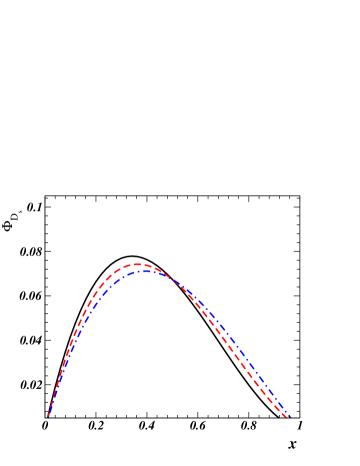
Figure 3: The wave function of $\Phi_{D_{s}}$ with $c_{D_{s}}=0.9$ (solid line), $c_{D_{s}}=0.7$ (dashed line), and $c_{D_{s}}=0.5$ (dashed-dotted line).

Finally, some remarks are given. In this paper, we assume that the mechanism of the color transparency Bjorken still dominates in $B$ decaying to charmed mesons so that we don’t have to consider the rescattering effects. From our results, we know that the PQCD approach can match the experimental data of the $B_{d}\to D^{-}_{s}K^{+}$ decay. With the same approach, our predictions on other decays, arising also from annihilation topologies, should be reliable. We note that the relevant charged $B$ decays of $B^{+}\to D^{(*)+}_{s}\bar{K}^{(*)0}$ are also governed by annihilation contributions. Due to the suppression of CKM matrix elements, $V_{ub}V^{*}_{cd}$, the BRs are estimated to be of ${\cal O}(10^{-8})$ LU . Since the corresponding nonresonant three-body final states $D^{(*)+}_{s}K^{-}\pi^{+}$ are also suppressed by the same CKM matrix elements, illustrated by Fig. 4, $B^{+}\to D^{(*)+}_{s}K^{-}\pi^{+}$ decays cannot give us more interesting information on three-body decays.

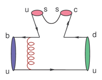
Figure 4: Topology for nonresonant three-body decays $B^{+}\to D_{s}^{(*)+}K^{-}\pi^{+}$.

Acknowledgments:

The author would like to thank H.N. Li, H.Y. Cheng, C.K. Chua, K.C. Yang, W.S. Hou, C.D. Lu and K. Ukai for their useful discussions. This work was supported in part by the National Science Council of the Republic of China under Grant No. NSC-91-2112-M-001-053 and the National Center for Theoretical Sciences of R.O.C..

References

(1) Belle Collaboration, A. Garmash et al., Phys. Rev. D65, 092005
(2002); A.Satpathy et al., hep-ex/0211022.
(2)B. Bajc et al., Phys. Lett. B447, 313
(1999); A. Deandrea et al., Phys. Rev. D62, 036001
(2000); A. Deandrea and A.D. Polosa, Phys. Rev. Lett. 86,
216 (2001); J. Tandean and S. Gardner, Phys. Rev. D66,
034019 (2002).
(3)C.H. Chen, Phys. Rev. D67,014012 (2003).
(4) C.K. Chua, W.S. Hou and S.Y. Tsai, Phys. Lett. B544, 139 (2002).
(7) A. Drutskoy et al., Phys. Lett. B 542, 171
(2002).
(8)
V.E. Balakin et al., Phys. Lett. B41, 205 (1972); M.
Bernardini et al., Phys. Lett. B44, 393 (1973); 46, 261 (1973); B. Delcourt et al., Phys. Lett. B99,
257 (1981); P.M. Ivanov et al., Phys. Lett. B 107, 297
(1981); DM2 Collaboration, D. Bisello et al., Z. Phys. C39, 13 (1988); F. Mane et al., Phys. Lett. B99, 261
(1981); S.I. Dolinsky et al., Phys. Rept. 202, 99
(1991); R. R. Akhmetshin et al., Phys. Lett. B364, 199
(1995).
(9)C.K. Chua, W.S. Hou, S.Y. Shiau and S.Y. Tsai,
hep-ph/0209164.
(10) D. Muller et al., Fortschr. Physik. 42, 101 (1994);
M. Diehl, T. Gousset, B. Pire, and O. Teryaev, Phys. Rev. Lett.
81, 1782 (1998); M.V. Polyakov, Nucl. Phys. B555, 231
(1999).
(11) Belle Collaboration, P. Krokovny et al.,
Phys. Rev. Lett. 89, 231804 (2002).
(12) Babar Collaboration, B. Aubert, et al.,
hep-ex/0207053.
(13) N. Cabibbo, Phys. Rev. Lett. 10, 531 (1963); M.
Kobayashi and T. Maskawa, Prog. Theor. Phys. 49, 652 (1973).
(14) G. Buchalla , A.J. Buras and M.E. Lautenbacher,
Rev. Mod. Phys. 68, 1230 (1996).
(15) G.P. Lepage and S.J. Brodsky, Phys. Lett. B87, 359
(1979); Phys. Rev. D22, 2157 (1980).
(16) H.N. Li, Phys. Rev. D64, 014019 (2001).
(17) T. Kurimoto, H.N. Li and A.I. Sanda, Phys. Rev. D65, 014007 (2002).