NUCLEON STRANGENESS IN DISPERSION THEORY

Abstract

Dispersion relations provide a powerful tool to describe the low-energy structure of hadrons. We review the status of the strange vector form factors of the nucleon in dispersion theory. We also comment on open questions and the relation to chiral perturbation theory.

1 Introduction

The low-energy structure of the nucleon’s $\bar{s}s$ sea is an important topic in hadron physics[1, 2]. While deep inelastic scattering has provided information about the light-cone momentum distribution of the strange sea[3], little is known about the corresponding spatial and spin distributions or about the role played by the sea in the nucleon’s response to a low-energy probe. Parity-violating experiments with polarized electrons can be used to probe nucleon matrix elements of the strange-quark vector current, which is parametrized by the strange electric and magnetic form factors ${G_{E}^{s}}$ and ${G_{M}^{s}}$, respectively. In an effort to measure these form factors, several such experiments have been carried out or are under way at MIT-Bates (SAMPLE), Jefferson Lab (HAPPEX, G0), and Mainz (A4). These experiments have produced the first measurements of ${G_{M}^{s}}$ [4], as well as a linear combination of ${G_{M}^{s}}$ and ${G_{E}^{s}}$ [5].

Since the strange quark mass is of the order of $\Lambda_{QCD}$, calculating the strange vector form factors is a complex problem that crucially depends on the nonperturbative aspects of QCD. A variety of approaches have been used to calculate the leading strange moments in the past: lattice QCD, chiral perturbation theory, a plethora of hadronic models, and dispersion relations. Most calculations agree neither in sign nor in magnitude. This reflects the difficulty in calculating $SU(3)$ flavor singlet observables which are not constrained by the mainly electromagnetic data available. In this talk, I will focus on what has been learned using dispersion relations (DR’s). After a brief review of the formalism in Sec. 2, I will discuss the dispersion theory calculations of the strange vector form factors in Sec. 3. Section 4 deals with the connection to chiral perturbation theory and Sec. 5 contains the conclusions. For a discussion of the other approaches, see the talks by Pene, Riska, and Holstein, as well as the recent review article by Beck and Holstein[2].

2 Formalism

Using Lorentz and gauge invariance, the nucleon matrix element of the strange vector current operator $\bar{s}\gamma_{\mu}s$ can be parametrized in terms of two form factors,

$$\langle N(p^{\prime})|\bar{s}\gamma_{\mu}s|N(p)\rangle=\bar{u}(p^{\prime})\left[{F_{1}^{s}}(t)\gamma_{\mu}+\frac{i}{2M}{F_{2}^{s}}(t)\sigma_{\mu\nu}q^{\nu}\right]u(p)\,,$$ (1)

where $M$ is the nucleon mass and $t=(p^{\prime}-p)^{2}=q^{2}$ the four-momentum transfer. In electron scattering, the form factors are probed at spacelike $t<0$. ${F_{1}^{s}}$ and ${F_{2}^{s}}$ are the Dirac and Pauli form factors, respectively. ${F_{1}^{s}}$ vanishes at $t=0$ since the net strangeness of the nucleon is zero, while ${F_{2}^{s}}$ is normalized to the anomalous strange magnetic moment of the nucleon, $\kappa^{s}$. The experimental data are usually given for the Sachs form factors, which are linear combinations of the Dirac and Pauli form factors:

$${G_{E}^{s}}(t) = {F_{1}^{s}}(t)-\tau{F_{2}^{s}}(t)\,,\qquad{G_{M}^{s}}(t)={F_{1}^{s}}(t)+{F_{2}^{s}}(t)\,,$$ (2)

where $\tau=-t/(4M^{2})$. In the Breit frame, ${G_{E}^{s}}$ and ${G_{M}^{s}}$ may be interpreted as the Fourier transforms of the distribution of strangeness charge and magnetization, respectively. Most theoretical calculations have focused on the leading moments of the form factors,

$$\kappa^{s}={F_{2}^{s}}(0)\,, \mu^{s}={G_{M}^{s}}(0)\,,$$

$$\langle r^{2}\rangle_{D}^{s}=6\frac{d{F_{1}^{s}}}{dt}\bigg{|}_{t=0}\,, \langle r^{2}\rangle_{E/M}^{s}=6\frac{dG_{E/M}^{s}}{dt}\bigg{|}_{t=0}\,.$$ (3)

Note also that $\mu^{s}\equiv\kappa^{s}$ since ${F_{1}^{s}}(0)=0$.

3 Strange Vector Form Factors in Dispersion Theory

3.1 Spectral Decomposition

Based on unitarity and analyticity, dispersion relations (DR’s) relate the real and imaginary parts of the strange vector form factors. Consider, e.g., the Pauli form factor ${F_{2}^{s}}$. We write down an unsubtracted DR of the form

$${F_{2}^{s}}(t)=\frac{1}{\pi}\,\int_{t_{0}}^{\infty}\frac{{\rm Im}\,{F_{2}^{s}}(t^{\prime})}{t^{\prime}-t-i\epsilon}\,dt^{\prime}\,,$$ (4)

where $t_{0}=9{m_{\pi}^{2}}$ is the threshold of the lowest cut of ${F_{2}^{s}}$. In the case of ${F_{1}^{s}}$, the value of the form factor at $t=0$ is known and a once subtracted DR can be used. By performing more subtractions, the sensitivity to the imaginary part at high momentum transfer can be reduced and the convergence behavior of the DR improved. Even though some information about the large-$t$ behavior is available from perturbative QCD and Regge fits, the question of whether a given DR converges remains an assumption and can not be answered a priori. The imaginary part or spectral function entering Eq. (4) can be obtained from a spectral decomposition[6, 7]. For this purpose, it is convenient to consider the strange vector current matrix element in the timelike region,

$$J_{\mu} = \langle N(p)\overline{N}(\bar{p})|\bar{s}\gamma_{\mu}s|0\rangle$$ (5)

$$= \bar{u}(p)\left[{F_{1}^{s}}(t)\gamma_{\mu}+\frac{i}{2M}{F_{2}^{s}}(t)\sigma_{\mu\nu}(p+\bar{p})^{\nu}\right]v(\bar{p})\,,$$

where $p\,,\bar{p}$ are the momenta of the nucleon-antinucleon pair created by the current $\bar{s}\gamma_{\mu}s$. The four-momentum transfer in the timelike region is $t=(p+\bar{p})^{2}>0$. Using the LSZ formalism, the imaginary part of the form factors is obtained by inserting a complete set of intermediate states[6, 7]

$${\rm Im}\,J_{\mu} = \frac{\pi}{\sqrt{Z}}(2\pi)^{3/2}{\mathcal{N}}\,\sum_{n}\langle p|\bar{J}_{N}(0)|n\rangle\langle n|\bar{s}\gamma_{\mu}s|0\rangle\,v(\bar{p})\,\delta^{4}(p+\bar{p}-p_{n})\,,$$ (6)

where ${\mathcal{N}}$ is a nucleon spinor normalization factor, $Z$ is the nucleon wave function renormalization, and $\bar{J}_{N}(x)=J^{\dagger}(x)\gamma_{0}$ with $J_{N}(x)$ a nucleon source.

Figure 1: Graphical illustration of the spectral decomposition in Eq. (6). The intermediate states $|n\rangle$ are on shell.

The spectral decomposition in Eq. (6) is illustrated in Fig. 1. The states $|n\rangle$ are asymptotic states of momentum $p_{n}$ and therefore on shell. They are stable with respect to the strong interaction. Only intermediate states that carry the same quantum numbers as the current $\bar{s}\gamma_{\mu}s$ [$I^{G}(J^{PC})=0^{-}(1^{--})$, baryon number zero, and no net strangeness] contribute to the sum in Eq. (6). The lowest-mass states satisfying this criterion are: $3\pi$, $5\pi$, $\ldots$, $K\bar{K}$, $K\bar{K}\pi$, $K\bar{K}\pi\pi$, $\ldots$, $\Lambda\bar{\Lambda}$, $\Sigma\bar{\Sigma}$, $\ldots$. Because of $G$-parity, only states with an odd number of pions contribute. Associated with each intermediate state is a cut starting at the corresponding threshold in $t$ and running to infinity. As a consequence, the spectral functions ${\rm Im}\,F_{i}^{s}(t),\;i=1,2$ are different from zero along the cut from $t_{0}=9\,m_{\pi}^{2}$ to $\infty$. Using Eqs. (5,6), the spectral functions can in principle be constructed from experimental data. In practice, this proves a formidable task and has only been done for the $K\bar{K}$-continuum contribution, as will be discussed in Sec. 3.3. However, the spectral function can also be modelled by using vector meson dominance.

3.2 Vector Meson Dominance

Within the vector meson dominance (VMD) approach, the spectral functions are approximated by a few vector meson poles, namely the $\omega,\phi,\ldots$. In that case, the strange vector form factors take the form

$$F_{i}^{s}(t)=\sum_{V=\omega,\phi,...}\frac{a_{i}^{V}}{m^{2}_{V}-t}\,,\qquad i=1,2\,.$$ (7)

Clearly, such pole terms contribute to the spectral functions as $\delta$-functions,

$${\rm Im}\,F^{s}_{i}(t)=\pi\,\sum_{V=\omega,\phi,...}a_{i}^{V}\,\delta(t-m_{V}^{2})\,,\qquad i=1,2\,.$$ (8)

These terms arise naturally as approximations to vector meson resonances in the continuum of intermediate states like $n\pi$ ($n\geq 3)$, $K\overline{K}$ and so on. If the continuum contributions are strongly peaked near the vector meson resonances, Eq. (8) is a good approximation to the true spectral function.

A dispersion analysis of the nucleon’s electromagnetic form factors with three vector meson poles in both the isoscalar and isovector channels as well as the two-pion continuum in the isovector channel was carried out by Höhler et al.[8]. In this analysis the isoscalar electromagnetic form factors were parametrized by three vector meson resonances: $\omega$, $\phi$, and a third fictitious $S^{\prime}$ meson with a mass of about $1.6$ GeV. The $S^{\prime}$ effectively summarizes higher mass strength in the spectral function.

The first application of this framework to the strange vector form factors was carried out by Jaffe[9]. He used the knowledge of the flavor content of the $\omega$ and $\phi$ mesons to deduce their coupling to the strange vector current from their coupling to the isoscalar electromagnetic current by performing a rotation in flavor space. The underlying principle is very simple: The flavor content of the $\omega$ and $\phi$ mesons can be written as:

$$|\phi\rangle\approx|s\bar{s}\rangle\,,\qquad|\omega\rangle\approx\frac{1}{\sqrt{2}}(|u\bar{u}\rangle+|d\bar{d}\rangle)\,,$$ (9)

while the isoscalar electromagnetic quark current is simply

$$j_{\mu}^{\rm is}=\frac{1}{6}\left(\bar{u}\gamma_{\mu}u+\bar{d}\gamma_{\mu}d\right)-\frac{1}{3}\bar{s}\gamma_{\mu}s\,,$$ (10)

if the heavier $c$, $b$, and $t$ quarks are neglected. The OZI rule then leads to the relations

$$\langle 0|\bar{s}\gamma_{\mu}s|\omega\rangle\approx 0\,,\qquad\langle 0|\bar{u}\gamma_{\mu}u+\bar{d}\gamma_{\mu}d|\phi\rangle\approx 0\,,$$ (11)

which can be used to determine the coupling of the $\omega$ and $\phi$ mesons to the strange vector current. If $\omega-\phi$-mixing and the phenomenological OZI violation are also included, one finds[17]

$$\langle 0|\bar{s}\gamma_{\mu}s|\phi\rangle\approx-3\langle 0|j_{\mu}^{\rm is}|\phi\rangle\,,\qquad\langle 0|\bar{s}\gamma_{\mu}s|\omega\rangle\approx-0.2\langle 0|j_{\mu}^{\rm is}|\omega\rangle\,,$$ (12)

which lead to a relation between the pole residues $a_{i}^{V}$ for the strange vector and isoscalar electromagnetic currents. The coupling of the fictitiuos $S^{\prime}$ meson, however, can not be deduced this way since its flavor content is unknown. Furthermore, it is not guaranteed that the strange vector form factor can be described using the same three poles as for the isoscalar electromagnetic form factors. Casting this issue aside, one can determine the coupling of the $S^{\prime}$ meson by fixing the asymptotic behavior of the form factors. (But note that this procedure is not unique and leads to an ambiguity in the leading moments[10].) Using the electromagnetic form factor analysis of Höhler et al.[8], Jaffe determined the the leading moments $\mu^{s}$ and $\langle r^{2}\rangle_{D}^{s}$ of the strange form factors[9]. In particular, his analysis gave a large strange magnetic moment. This was due to the strong coupling of the $\phi$ to the nucleon in electromagnetic analyses[8, 11], where a second pole around $t=1.0$ GeV² in addition to the $\omega$ is required to generate the dipole behavior of the data. Usually this pole is identified with the $\phi$, which implies a large OZI violation.

Since the electromagnetic form factor analysis[8] is over 20 years old and does not include the precise data from later experiments, it was recently updated and improved[11]. Subsequently, we have performed an updated analysis of the strange vector form factors based on the new electromagnetic data[12]. The results for leading moments are

$$\mu^{s}=-0.24\pm 0.03\,,\qquad\langle r^{2}\rangle_{D}^{s}=(0.21\pm 0.03)\mbox{ fm}^{2}\,,$$ (13)

where the error includes only the uncertainty in the phenomenological $\phi-\omega$-mixing parameter $\epsilon$. The systematic error from using the pole ansatz for the spectral function is difficult to quantify.

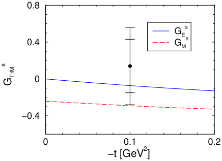
Figure 2: Strange vector form factors from the updated pole analysis[12]. The data point for $G_{M}^{s}$ is from the SAMPLE collaboration[4]. The inner error bar is statistical, while the outer error bar combines statistical and systematic errors in quadrature.

In Fig. 2, we show the results of this analysis compared to the data point for ${G_{M}^{s}}$ from the SAMPLE collaboration[4]. The calculation breaks down at higher momentum transfers. If it is nevertheless extrapolated to larger $t$, it disagrees with the measurement of the combination $G_{E}^{s}+0.39G_{M}^{s}$ at $t=-0.48$ GeV² by the HAPPEX collaboration[5].

As noted above, it is not clear whether the simple three pole approximation for ${F_{1}^{s}}$ and ${F_{2}^{s}}$ is justified. In the case of the isovector electromagnetic form factors, e.g., there is an important contribution from the $\pi\pi$ continuum[13, 14]. The left hand shoulder of the $\rho$ resonance is enhanced because of a singularity on the unphysical sheet close to the physical region at $t_{c}=4{m_{\pi}^{2}}-{m_{\pi}^{2}}/M^{2}$. The prime candidates for large continuum contributions to the strange form factors are the $3\pi$ and $K\bar{K}$ states, which are the lightest intermediate states containing nonstrange and strange particles, respectively. However, it was shown that there is no threshold enhancement in the $3\pi$ continuum[15]. As a consequence, we focus on the $K\bar{K}$ continuum in the next section.

3.3 $K\bar{K}$-Continuum

In order to determine $K\bar{K}$ contribution to the spectral functions in Eq. (6), we need the matrix elements ${\langle N(p)|}\bar{J}_{N}(0){|K(k)\bar{K}(\bar{k})\rangle}\,v(\bar{p})$ and ${\langle K(k)\bar{K}(\bar{k})|}\bar{s}\gamma_{\mu}s{|0\rangle}$.

3.3.1 Unitarity Bounds

By expanding the $K\bar{K}\to N\bar{N}$ amplitude in partial waves, we are able to impose the constraints of unitarity in a straightforward way. In doing so, we use the helicity formalism[16]. With $\lambda$ and $\bar{\lambda}$ being the nucleon and antinucleon helicities, we write the corresponding $S$-matrix element as

$${\langle N(p,\lambda)\bar{N}({\bar{p}},\bar{\lambda})|}{\hat{S}}{|K(k)\bar{K}(\bar{k})\rangle}=$$ (14)

$$\hphantom{N(p,\lambda)}i(2\pi)^{4}\delta^{4}(p+{\bar{p}}-k-\bar{k})(2\pi)^{2}\left[{64t\over t-4m_{K}^{2}}\right]^{1/2}{\langle\theta,\phi,\lambda,\bar{\lambda}|}{\hat{S}}(P){|00\rangle}\,,$$

where $t=P^{2}=(p+{\bar{p}})^{2}$ and $m_{K}$ is the kaon mass. The matrix element ${\langle\theta,\phi,\lambda,\bar{\lambda}|}{\hat{S}}(P){|00\rangle}$ is then expanded in partial waves as[16, 7]

$$S_{\lambda,\bar{\lambda}}\equiv{\langle\theta,\phi,\lambda,\bar{\lambda}|}{\hat{S}}(P){|00\rangle}=\sum_{J}\left({2J+1\over 4\pi}\right)b_{J}^{\lambda,\bar{\lambda}}\;{\mathcal{D}}_{0\mu}^{J}(\phi,\theta,-\phi)^{\ast}\,,$$ (15)

where ${\mathcal{D}}_{\nu\,\nu^{\prime}}^{J}(\alpha,\beta,\gamma)$ is a Wigner rotation matrix with $\mu=\lambda-\bar{\lambda}$. The $b_{J}^{\lambda\,\bar{\lambda}}$ define partial waves of angular momentum $J$. Only the $J=1$ partial waves contribute to the spectral functions for vector currents. Moreover, because of parity invariance only two of the four partial waves for $J=1$ are independent. Choosing ${b_{1}^{1/2,\,1/2}}$ and ${b_{1}^{1/2,\,-1/2}}$, the unitarity of the $S$-matrix, $S^{{\dagger}}S=1$, requires that

$$^{4}\!\!\sqrt{\frac{t-4M^{2}}{t-4{m_{K}^{2}}}}\left|b_{1}^{1/2,\pm 1/2}(t)\right|\leq 1\,,$$ (16)

for $t\geq 4{M^{2}}$. Consequently, unitarity provides model-independent bounds on the contribution of the physical region ($t\geq 4{M^{2}}$) to the imaginary part. To evaluate the DR, however, the ${b_{1}^{1/2,\,\pm 1/2}}$ are also needed in the unphysical region ($4{m_{K}^{2}}\leq t\leq 4{M^{2}}$), where they are not bounded by unitarity. Instead, we must rely upon an analytic continuation to obtain the ${b_{1}^{1/2,\,\pm 1/2}}$ in the unphysical region.

3.3.2 Analytic Continuation

A detailed discussion of the analytic continuation procedure and its problems can be found elsewhere[17], here we only give a brief overview. To obtain the $b_{1}^{1/2,\pm 1/2}$ for $4{m_{K}^{2}}\leq t\leq 4{M^{2}}$, we analytically continue physical amplitudes into the unphysical regime. However, the analytic continuation (AC) of a finite set of experimental data with non-zero error is fraught with potential ambiguities. Indeed, the AC is inherently unstable, and analyticity alone has no predictive power. Additional information must be used in order to stabilize the problem.

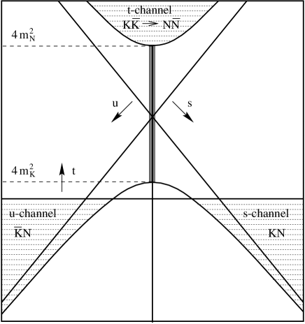
Figure 3: Mandelstam plane for $KN$ scattering. Physical regions are marked by dashed areas.

In order to illustrate these issues and the methods we adopt to resolve them, we first briefly review the kinematics of $KN$ scattering. It is useful to consider the $s$-, $u$-, and $t$-channel reactions simultaneously,

(a) $$s \qquad K(q_{i})+N(p_{i})\rightarrow K(q_{f})+N(p_{f})\,,$$-channel: (17)

(b) $$u \qquad\bar{K}(-q_{f})+N(p_{i})\rightarrow\bar{K}(-q_{i})+N(p_{f})\,,$$-channel:

(c) $$t \qquad\bar{K}(-q_{f})+K(q_{i})\rightarrow\bar{N}(-p_{i})+N(p_{f})\,,$$-channel:

where the four-momenta of the particles are given in parentheses. In this notation the crossing relations between the different channels are immediately transparent. The three processes can be described in terms of the usual Mandelstam variables $s=(p_{i}+q_{i})^{2}\,$, $u=(p_{i}-q_{f})^{2}\,$, and $t=(q_{i}-q_{f})^{2}\,$. The ranges of $s,u,$ and $t$ in the Mandelstam plane are shown in Fig 3. The invariant amplitudes are defined in the whole plane and simultaneously describe all three processes in the physical regions marked by the dashed areas. The physical values of the invariant amplitudes are obtained when the Mandelstam variables are taken in the corresponding ranges. In order to carry out the dispersion integrals, we require the ${b_{1}^{1/2,\,\pm 1/2}}$ along the $t$-channel cut in the unphysical region. This is the gray shaded area in Fig. 3 where the unitarity bounds do not apply.

We begin with experimental $KN$ amplitudes in the s-channel region[18] and employ the method of backward DR to obtain the unphysical amplitudes along the $t$-channel cut. In order to stabilize the numerical continuation, we subtract the rapidly varying nucleon pole terms which are known analytically. We also divide out the asymptotic behavior of the amplitudes. We analytically continue the remainder using backwards DR’s, reinstate the asymptotic behavior, and add the pole terms afterwards. The results[17] for the amplitudes ${b_{1}^{1/2,\,\pm 1/2}}$ are shown in Fig. 4.

Figure 4: Analytically continued amplitudes ${b_{1}^{1/2,\,\pm 1/2}}$. The dashed line indicates the real part, the dotted line indicates the imaginary part, and the solid line shows the absolute value.

The analytic continuation ist trustworthy up to $t\approx 2.0$ GeV². A clear resonance signature in ${b_{1}^{1/2,\,1/2}}$, presumably the $\phi$ resonance, is seen at the $K\bar{K}$ threshold.

3.3.3 Kaon Strangeness Form Factor

The second matrix element appearing in Eq. (6), ${\langle K(k)\bar{K}(\bar{k})|}\bar{s}\gamma_{\mu}s{|0\rangle}$, is parametrized by the kaon strangeness form factor ${F_{K}^{s}}$:

$${\langle 0|}\bar{s}\gamma_{\mu}s{|K(k)\bar{K}(\bar{k})\rangle} = (k-\bar{k})_{\mu}{F_{K}^{s}}(t)\,.$$ (18)

To obtain ${F_{K}^{s}}(t)$ we draw upon the known flavor content of the vector mesons. We use the flavor rotation arguments discussed in Sec. 3.2 to obtain the strangeness form factor from various parametrizations for the electromagnetic kaon form factors[7, 17]. This procedure should give a reliable estimate since the kaon has net strangeness.

The timelike kaon form factor is dominated by the $\phi(1020)$ resonance. We note that the flavor rotation applied to the electromagnetic form factor only gives the relative size of the $\omega$ and $\phi$ contributions, but does not lead to the correct normalization ${F_{K}^{s}}(0)=-1$ which must be enforced by hand.

Figure 5: Different model parametrizations for ${F_{K}^{s}}$. Full line shows simple VMD model with the $\phi$ only, dashed line shows the flavor rotated VMD model including the $\omega$ and $\phi$, and dash-dotted line shows Gounaris-Sakurai parametrization. $K\bar{K}$ threshold is at $t\approx 1.0$ GeV².

In Fig. 5 we plot ${F_{K}^{s}}$ extracted from three different models for the electromagnetic form factor one of which includes a contribution from the $\omega$. We observe that all models reproduce the essential features of ${F_{K}^{s}}$ as determined from $e^{+}e^{-}$ data and standard flavor rotation arguments. Since ${F_{K}^{s}}$ is needed for $t\geq 4{m_{K}^{2}}$, the $\omega$-contribution which gives rise to the bump around $t\approx 0.6\mbox{ GeV}^{2}$ in Fig. 5 is irrelevant for our purpose. When computing the leading strangeness moments, we find a less than 10% variation in the results when any of these different parametrizations for ${F_{K}^{s}}$ is used.

3.3.4 $K\bar{K}$ Spectral Function

The exact relation of the spectral functions to the partial waves and the kaon strangeness form factor is[7]

$${\rm Im}\,{F_{1}^{s}}(t) = {\rm Re}\,\left\{{{M}q_{t}\over 4p_{t}^{2}}\left[{E\over\sqrt{2}{M}}{b_{1}^{1/2,\,-1/2}}(t)-{b_{1}^{1/2,\,1/2}}(t)\right]{F_{K}^{s}}(t)^{\ast}\right\}\,,$$ (19)

$${\rm Im}\,{F_{2}^{s}}(t) = {\rm Re}\,\left\{{{M}q_{t}\over 4p_{t}^{2}}\left[{b_{1}^{1/2,\,1/2}}(t)-{{M}\over\sqrt{2}E}{b_{1}^{1/2,\,-1/2}}(t)\right]{F_{K}^{s}}(t)^{\ast}\right\}\,,$$ (20)

where $p_{t}=\sqrt{t/4-{M^{2}}}\,$, $q_{t}=\sqrt{t/4-m_{K}^{2}}\,$, and $E=\sqrt{t}/2\,$.

On one hand, Eqs. (19,20) may be used to determine the spectral functions from experimental data. On the other hand, one can impose bounds on the imaginary parts in the physical region by using Eq. (16). In order to obtain finite bounds for the Dirac and Pauli form factors at the $N\bar{N}$ threshold, we build in the correct threshold relation for the ${b_{1}^{1/2,\,\pm 1/2}}$, ${b_{1}^{1/2,\,-1/2}}(t=4{M^{2}})=\sqrt{2}{b_{1}^{1/2,\,1/2}}(t=4{M^{2}})$. This is necessary to cancel the $1/p_{t}^{2}$ factor in Eqs. (19,20). Strictly speaking, the relation holds only for $t=4{M^{2}}$. For simplicity, however, we assume this relation to be valid for all momentum transfers. Consequently, we have[7]

$$|{\rm Im}\,{F_{1}^{s}}(t)| \leq \frac{q_{t}^{3/2}}{2\sqrt{2p_{t}}(\sqrt{t}+2{M})}|{F_{K}^{s}}(t)|\,,$$ (21)

$$|{\rm Im}\,{F_{2}^{s}}(t)| \leq \frac{2{M}}{\sqrt{t}}\frac{q_{t}^{3/2}}{2\sqrt{2p_{t}}(\sqrt{t}+2{M})}|{F_{K}^{s}}(t)|\,.$$ (22)

Similar expressions can be obtained for the Sachs form factors.

In Fig. 6, we show the spectral function of the DR for

Figure 6: Spectral functions for the electric (left panel) and magnetic radii (right panel). Solid line shows analytical continuation, dashed line shows unitarity bound, and dash-dotted line shows 1-loop result in the nonlinear $SU(3)$ sigma-model.

the electric and magnetic radii as an example[17]. We compare the analytical continuation (solid line) for $4{m_{K}^{2}}\leq t\leq 4{M^{2}}$ and the unitarity bound (dashed line) for $t\geq 4{M^{2}}$ to the 1-loop result in the nonlinear $SU(3)$ sigma-model (dash-dotted line). Clearly the perturbative 1-loop result misses the resonance structure at threshold. Furthermore, it strongly overestimates the contribution in the physical region since rescattering contributions are neglected. These results cast serious doubts on the reliability of any 1-loop model calculation of the strange form factors.

In order to calculate the strange form factors, one needs the contribution of all low-mass intermediate states in Eq. (6). In principle it would be desirable to perform a full dispersion calculation for all those states. Since, at present, this is not possible due to the lack of suitable experimental data, we combine the $K\bar{K}$ continuum with the pole approximation for the remaining low-mass states in the next section.

3.4 Low-mass Contributions

To make the connection to the leading strange moments, we merge the pole approximation with the exact $K\bar{K}$ continuum derived in the previous section[19]. The first step is to refit the isoscalar electromagnetic form factors in order to see how much of the original $\phi$ pole strength is provided by the $K\bar{K}$ continuum. We find that in $F_{2}$ all original $\phi$ strength can be accounted for by the $K\bar{K}$ continuum, while for $F_{1}$ some residual $\phi$ pole strength is required. This result justifies the identification of the pole around $t=1.0$ GeV² in electromagnetic analyses with the $\phi$[8, 11]. The additional $\phi$ pole strength in $F_{1}$ could be due to a $\rho\pi$ resonance which couples to the $\phi$. [Note that the branching ratio for the decay mode $\phi\to\rho\pi$ is 12%.]

In order to elucidate the consequences for the strange moments, we obtain the $\omega$ and residual $\phi$ contributions to the strange form factors from a flavor rotation. The $K\bar{K}$ continuum contribution which contains most of the $\phi$ strength is fixed from Sec. 3.3. However, the coupling of the $S^{\prime}$ to strangeness is still unknown. In order to avoid the ambiguity from the asymptotic condition used previously[9, 12], we allow a maximal coupling of the $S^{\prime}$ to the strange current and assess the uncertainty from varying the sign of this coupling. For the leading strange moments, we define a low-mass value. It contains the $\omega$, $\phi$, and $K\bar{K}$ contributions which are reasonably well under control. Adding the $S^{\prime}$ contribution, leads to a reasonable range, which quantifies the error in the unknown coupling of the $S^{\prime}$. Systematic errors from using the pole approximation, however, can not be quantified this way. The results[19] for the leading moments are shown in Table 1.

Table 1:

Table 1. Leading strange moments from $K\bar{K}$ continuum plus $\omega$, $\phi$, and $S^{\prime}$ poles.

Moment low-mass value reasonable range $\mu^{s}$ $-0.28$ $-0.15...-0.41$ $\langle r^{2}\rangle_{D}^{s}$ $0.42$ fm² $(0.41...0.43)$ fm² $\langle r^{2}\rangle_{M}^{s}$ $0.34$ fm² $(0.32...0.36)$ fm²

The magnetic moment seems to be most sensitive to the sign of the $S^{\prime}$ coupling and varies by a factor of two, while the radii are relatively stable. Compared to the pole analysis without the $K\bar{K}$ continuum, the Dirac radius is somewhat larger. The magnetic moment can be smaller but still remains clearly negative.

4 Connection to ChPT

In this section we illustrate how the dispersion results can be combined with chiral perturbation theory (ChPT). In ChPT, the strange moments $\mu^{s}$, $\langle r^{2}\rangle_{D}^{s}$, and $\langle r^{2}\rangle_{E}^{s}$ depend to leading order in the chiral expansion (LO) on unknown counterterms[20] and can at present not be predicted. Hemmert et al.[21] have shown that the strange magnetic radius $\langle r^{2}\rangle_{M}^{s}$ is independent of unknown counterterms at LO. Furthermore, for the magnetic form factor, they derived a model independent relation between the strange and isoscalar electromagnetic form factor. This leads to the LO prediction:

$$\langle r^{2}\rangle_{M}^{s}=(-0.16\ldots-0.60)\mbox{ fm}^{2}\,.$$ (23)

These numbers appear not to be compatible with the DR result from the previous section. They have been used to extrapolate the SAMPLE measurement of $G_{M}^{s}$ to $t=0$ in order to extract the strange magnetic moment[4]. However, at the next order in the chiral expansion there is a new counterterm contribution to the magnetic radius. The coefficient $b_{s}^{r}$ of this counterterm is unknown. In order to find out whether the inconsistency with DR’s persists, we have extended the ChPT calculation to next-to-leading order (NLO)[22]. The result for the magnetic radius at NLO is

$$\langle r^{2}\rangle_{M}^{s} = -\left[0.04+0.3\,b_{s}^{r}(\mu=1.0\mbox{ GeV}^{2})\right]\mbox{ fm}^{2}\,,$$ (24)

where $\mu$ is the renormalization scale. The model independent contribution from LO gets almost exactly cancelled by the loop contribution at NLO. As a consequence, the strange magnetic radius at NLO is dominated by the counterterm $b_{r}^{s}$. We have determined $b_{r}^{s}$ from matching Eq. (24) to the DR result and found $b_{s}^{r}\approx-1.1\,$, which agrees with the expectation from dimensional analysis. Consequently, the DR result and the chiral expansion are consistent to NLO. Furthermore, due to the cancellation of the NLO and LO loop contributions, the range for $\langle r^{2}\rangle_{M}^{s}$ given in Eq. (23) is not reliable. In Fig. 7, we illustrate the sensitivity of the extrapolation of the SAMPLE measurement of ${G_{M}^{s}}$ to $Q^{2}\equiv-t=0$.

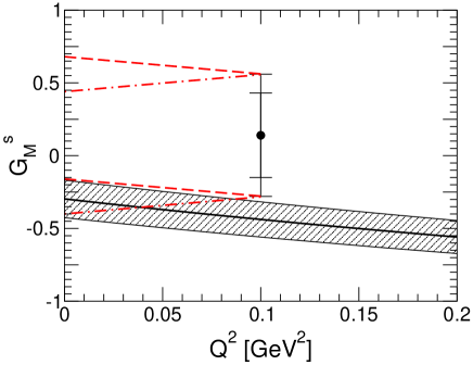
Figure 7: Error in extrapolation of ${G_{M}^{s}}$ to $Q^{2}\equiv-t=0$. Circle shows measurement of SAMPLE collaboration[4]. Dashed (dot-dashed) lines indicate extrapolation to $Q^{2}=0$ using $b_{s}^{r}=-1(+1)$. Solid line gives low-mass DR result, while shaded region indicates possible effects of higher mass states.

The dashed (dot-dashed) lines indicate extrapolation to $Q^{2}=0$ using $b_{s}^{r}=-1(+1)$, respectively. For comparison, the solid line gives low-mass DR result from Sec. 3.4, while shaded region indicates possible effects of higher mass states. Clearly, the error in the extrapolation to $Q^{2}=0$ is presently dominated by the statistical error of the experiment.

5 Conclusions

Dispersion theory has provided many insights into the structure of the nucleon’s strange vector form factors. In particular, the role of the $K\bar{K}$ continuum to the spectral function is now well understood. Drawing upon rigorous bounds from unitarity and an analytic continuation of $K\bar{K}\to N\bar{N}$ amplitudes, rescattering and resonance contributions were shown to be crucial for the $K\bar{K}$ contribution to the spectral function[7, 17]. This result casts doubt on any perturbative model calculation at the 1-loop level where these effects are not included. The apparent discrepancy in the magnetic radius between ChPT at LO and the dispersion relation result disappears at NLO where a new low-energy constant enters[22].

However, many open questions remain. Even though it is the most important state, the $K\bar{K}$ intermediate state is not the only relevant low-mass state contributing to the spectral function. At present, a full dispersion calculation for the other low-mass states (such as $3\pi,5\pi,...,K\bar{K}\pi,K\bar{K}\pi\pi,...$) is not feasible. Baryonic intermediate states are expected to be strongly suppressed by unitarity. For the mesonic low-mass states, one has to rely on the vector meson pole approximation. This introduces a systematic error that is difficult to quantify. In particular, there are some indications of a $\rho\pi$ resonance in the $3\pi$ continuum, as well $K^{*}$ resonance effects in the $K\bar{K}\pi$ and $K\bar{K}\pi\pi$ states. Finally, the large-$t$ behavior from perturbative QCD might provide useful constraints on the sum over intermediate states in the spectral function. More low-$t$ data on the nucleon’s strange vector form factors will be extremely useful in understanding these issues.

References

- [1] M.J. Musolf et al., Phys. Rep. 239, 1 (1994).
- [2] D.H. Beck and B.R. Holstein, Int. J. Mod. Phys. E 10, 1 (2001).
-
[3]
A.O. Bazarko et al., Z. Phys. C 65, 189 (1995);
S.A. Rabinowitz et al., Phys. Rev. Lett. 70, 134 (1993). - [4] R. Hasty, et al., SAMPLE Collaboration, Science 290, 2117 (2000).
- [5] K. Aniol et al., HAPPEX Collaboration, Phys. Lett. B 509, 211 (2001).
-
[6]
G.F. Chew et al., Phys. Rev. 110, 265 (1958);
P. Federbush, M. Goldberger, S. Treiman, Phys. Rev. 112, 642 (1958). - [7] M.J. Musolf, H.-W. Hammer, D. Drechsel, Phys. Rev. D 55, 2741 (1997); Erratum ibid. D 62, 079901 (2000).
- [8] G. Höhler et al., Nucl. Phys. B 114, 505 (1976).
- [9] R.L. Jaffe, Phys. Lett. B 229, 275 (1989).
- [10] M.J. Musolf, talk at the conference “Polarization in Electron Scattering”, Santorini, Greece, 1995; H. Forkel, Phys. Rev. C 56, 510 (1997).
-
[11]
P. Mergell, U.-G. Meißner, D. Drechsel,
Nucl. Phys. A 596, 367 (1996);
H.-W. Hammer, U.-G. Meißner, D. Drechsel, Phys. Lett. B 385, 343 (1996). - [12] H.-W. Hammer, U.-G. Meißner, D. Drechsel, Phys. Lett. B 367, 323 (1996).
- [13] W.R. Frazer and J.R. Fulco, Phys. Rev. 117, 1603 (1960); 117, 1609 (1960).
- [14] G. Höhler and E. Pietarinen, Phys. Lett. B 53, 471 (1975).
- [15] V. Bernard, N. Kaiser, U.-G. Meißner, Nucl. Phys. A 611, 429 (1996).
- [16] M. Jacob and G.C. Wick, Ann. Phys.(NY) 7, 404 (1959).
- [17] H.-W. Hammer and M.J. Ramsey-Musolf, Phys. Rev. C 60, 045205 (1999); Erratum ibid. C 62, 049903 (2000); M.J. Ramsey-Musolf and H.-W. Hammer, Phys. Rev. Lett. 80, 2539 (1998); Erratum ibid. 85, 224 (2000).
- [18] J.S. Hyslop et al., Phys. Rev. D 46, 961 (1992).
- [19] H.-W. Hammer and M.J. Ramsey-Musolf, Phys. Rev. C 60, 045204 (1999); Erratum ibid. C 62, 049902 (2000).
- [20] M.J. Ramsey-Musolf and H. Ito, Phys. Rev. C 55, 3066 (1997).
- [21] T.R. Hemmert, U.-G. Meißner, S. Steininger, Phys. Lett. B 437, 184 (1998).
- [22] H.-W. Hammer, S.J. Puglia, M. Ramsey-Musolf, S.-L. Zhu, hep-ph/0206301.