What mediates the longest correlation length in the QCD plasma?

Abstract

When thermal QCD crosses the critical temperature from below, its pressure density rises drastically, consistent with the picture of deconfinement and the release of partons as light degrees of freedom. On the other hand, the concept of partons is a perturbative one, whereas interactions with the infrared modes in the plasma always introduce non-perturbative contributions. Here I show how partonic correlators can be defined in a gauge invariant and non-perturbative manner which applies to all energy scales. In particular, I compute the magnetic mass for hot SU(2) gauge theory and find $m_{A}=0.36(2)g^{2}T$, whose inverse for large $T$ is the largest correlation length in the system.

1 Introduction

After many years of theoretical studies and well into the period of heavy ion collision experiments trying to establish the quark gluon plasma of QCD, we are still far from understanding which objects constitute the fundamental degrees of freedom in that phase, and what their properties are. Lattice simulations of the equation of state have provided firm evidence that the effective number of light degrees of freedom is growing rapidly across $T_{c}\sim 170$ MeV, as shown in Figure 1.

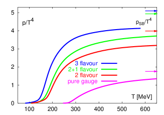
Figure 1: Temperature and flavor dependence of the QCD pressure density [1].

This conclusion can be drawn because the pressure rises with temperature for a theory with a given particle content, as well as with the number of light fermion flavors for all temperatures. In the naive deconfinement picture this is explained by the hadronic degrees of freedom dissolving into partons, for which one expects larger correlation lengths.

While this picture explains the qualitative features, the flattening of the pressure short of the ideal gas value indicates that up to $T\sim 4T_{c}$ interactions still play an important role. This in accord with the fact that the running gauge coupling at these temperatures is still large, and confirmed by detailed studies of screening masses in the plasma, which behave non-perturbatively: contributions from the soft magnetic modes $\sim g^{2}T$ overpower those of the electric modes $\sim gT$ at the temperatures in question [2]. Eventually the ideal gas pressure is obtained at asymptotically high temperatures [3], and the screening masses are dominated by the perturbative contributions. But even in this regime the soft modes $\sim g^{2}T$ are, through dimensional reduction [4], described by a 3d confining theory whose perturbation theory is infrared divergent (Linde problem) [5]. So we have evidence for the effective degrees of freedom getting more and lighter corresponding to some kind of constituent, but because of the interplay between soft and hard modes a purely perturbative parton picture is not appropriate.

To interpolate smoothly between hadronic and partonic regimes thus requires a non-perturbative study of the dynamics of color degrees of freedom which is valid for all scales. Color dynamics is encoded in Green functions of quarks and gluons, which in general are not gauge invariant. In perturbation theory one fixes a gauge and studies e.g. the field propagators directly. While these are not physical observables, they nevertheless carry physical information about the parton dynamics in their singularity structure. For example, the pole mass defined from the quark propagator is gauge independent and infrared finite to every finite order in perturbation theory [6]. A similar result holds for the gluon propagator, provided an appropriate resummation of infrared sensitive diagrams has been performed [7]. This has been used to define the Debye mass $m_{D}\sim gT$ in analogy to QED from the electric gauge field propagator [8]. Similarly, gauge invariant resummation schemes have been designed to self-consistently compute the pole of the gluon propagator in three dimensions [9]^-[12], corresponding to a “magnetic mass” regulating the non-abelian thermal infrared problem. However, it has so far not been clear whether these poles exist non-perturbatively.

On the other hand, on the lattice the study of partonic Green functions is hampered by several problems. It is difficult to fix a gauge uniquely and avoid the problem of Gribov copies [13]. Moreover, most complete gauge fixings (e.g. the Landau gauge) violate the positivity of the transfer matrix, thus obstructing a quantum mechanical interpretation of the results. For these reasons it has been argued to focus on correlators of local singlet operators only. A non-perturbative definition of the Debye mass in terms of singlet operators has been given [14], identifying it as the lowest screening mass in a singlet channel odd under Euclidean time reflection. The infrared cut-off on the magnetic scale $g^{2}T$ would in this picture be given by a 3d glueball mass. However, the corresponding correlation lengths are hadronic and not directly related to screening phenomena like e.g. $J/\psi$-suppression, which are caused by charged intermediate states[15].

In this contribution I want to demonstrate that non-perturbative and gauge invariant information is contained in an appropriately defined gluon two-point function, thus permitting to arrive at a field theoretical definition of an associated correlation length [16, 17]. Sections 2-4 show how to construct such an object which can be proved to decay with eigenvalues of the Hamiltonian. Section 5 relates the lowest eigenvalue to a level splitting between static mesons, which can be used to compute it without recourse to any gauge fixing at all. Such a computation is presented for SU(2) gauge theory in 3d. In Section 6 the result is compared to those from analytic resummation schemes, and argued to constitute the largest correlation length in the thermal system. Section 7 presents the conclusions.

2 A non-local gluon operator

A gauge invariant lattice gluon correlator can be defined when a complex $N$-plet transforming in the fundamental representation is available. One possibility is to take the eigenfunctions of the spatial covariant Laplacian, which is a hermitian operator with a positive spectrum,

$$-\left(D_{i}^{2}[U]\right)_{\alpha\beta}f^{(n)}_{\beta}(x)=\lambda_{n}f^{(n)}_{\alpha}(x),\quad\lambda^{n}>0.$$ (1)

They provide a unique mapping $U\rightarrow f[U]$ except when eigenvalues are degenerate or $|f|=0$. In simulations the probability of generating such configurations is essentially zero. These properties have been used previously for gauge fixing without Gribov copies and to construct blockspins for the derivation of effective theories [18]. The lowest eigenvectors are used to construct the matrix $\Omega(x)\equiv\frac{1}{|f(x)|}\left(f^{(1)}(x),f^{(2)}(x)\right)$, which transforms as $\Omega^{g}(x)=g(x)\Omega(x)h^{\dagger}(t)$. Composite link and gluon fields are defined by

$$V_{\mu}(x) = \Omega^{\dagger}(x)U_{\mu}(x)\Omega(x+\hat{\mu}),$$ (2)

$$A_{\mu}(x) = \frac{{\rm i}}{2g}\left[V_{\mu}(x)-V^{\dagger}_{\mu}(x)-\frac{1}{N}{\rm Tr\,}\left(V_{\mu}(x)-V^{\dagger}_{\mu}(x)\right)\right],$$ (3)

both transforming as $O_{i}^{g}(x)=h(t)O_{i}(x)h^{\dagger}(t)$, whereas $V_{0}^{g}(x)=h(t)V_{0}(x)h^{\dagger}(t+1)$. The gauge field at a given time now has only a global gauge freedom left. To cancel this in the correlator, the zero momentum projected time links $\tilde{V_{0}}(t)=\sum_{{\bf x}}V_{0}({\bf x},t)/|\sum_{{\bf x}}V_{0}({\bf x},t)|$ are multiplied to “strings” $\tilde{V}_{0}(t_{1},t_{2})$ connecting two timeslices. These ingredients can be combined to the gauge invariant operator

$$O[U]={\rm Tr\,}\left[A_{i}({\bf x},0)\tilde{V}_{0}(0,t)A_{i}({\bf x},t)\tilde{V}_{0}^{\dagger}(0,t)\right],$$ (4)

which in the particular gauge $V_{0}(t)=1$ reduces to the gluon propagator. Hence we have a gauge invariant non-local observable, which is identical to the gluon propagator in a particular gauge.

Using the transfer matrix formalism [19], this observable can be converted to a trace over quantum mechanical states, falling off exponentially as

$$\langle O[U]\rangle=\sum_{n}|\langle 0|\hat{A}_{\alpha\beta}({\bf x})|n^{L0}\rangle|^{2}{\rm e}^{-(E_{n}-E_{0})t}\;,$$ (5)

provided that there is a finite energy gap $(E_{1}-E_{0})$. The eigenvalues $E_{n}$ and eigenvectors $|n^{L0}\rangle$ are those of the Hamiltonian in Laplacian temporal gauge, $V_{0}(x)=1$. It has been proved [16] that this Hamiltonian has the same spectrum as the Kogut-Susskind Hamiltonian $\hat{H}_{0}$ [20], which is obtained by quantizing the theory in temporal gauge. Note that the zero momentum projection of the $V_{0}$ switches off the divergent self-energy of the sources, so the energies are finite.

3 Discussion and interpretation

One may now ask to what extent these results depend on the particular choice of $\Omega[U]$, which is not unique. It is crucial that $\Omega$ depends only on spatial links to preserve the transfer matrix. Clearly, any $\Omega\in SU(N)$ local in time and transforming in the same way permits construction of the gauge invariant observable Eq. (4). From the spectral representation it follows that all such observables fall off with the same spectrum, while $\Omega$ only enters the matrix elements representing the overlap of the operator with the eigenstates.

The construction of the composite link variable Eq. (2) may also be viewed as fixing Laplacian gauge on each timeslice. Our result then implies that all gauges satisfying the mentioned constraints (e.g. the standard lattice Coulomb gauge) will produce the same exponential decay. Fourier transforming Eq. (5) to momentum space, we obtain the non-perturbative analogue to the situation in perturbation theory: the energies appear as gauge invariant poles, while the matrix elements correspond to gauge dependent residues.

Note that this does not imply an asymptotically free colored state. The temporal links in the operator indicate the presence of static charges, as e.g. in a Wilson loop. In a Hamiltonian formulation [20, 19] the Kogut-Susskind Hamiltonian $\hat{H}_{0}$ acts on a Hilbert space $H_{0}$ of all complex, square integrable wave functions. Gauge invariant wave functions, $\psi[U^{g}]=\psi[U]$, form a subspace $H\subset H_{0}$, on which the gauge invariant projected Hamiltonian $\hat{H}$ acts. Generally, the spectrum of $\hat{H}$ consists of the physical particle states of the theory, which couple to local gauge invariant operators. In addition to these states, $\hat{H}_{0}$ contains also the spectrum of gauge field excitations in the presence of static sources, such as the static potential, gluelumps etc. These are gauge invariant energy eigenvalues to non-trivially transforming pure gauge wave functions. Full gauge invariance is restored once the source fields are made explicit. Our correlator thus probes a gauge field excitation with the quantum numbers of the gluon in the presence of sources, which do not contribute to the field energy.

4 A numerical check

It is expedient to first test this new operator in a 3d SU(2) Higgs model, which in its broken phase has physical states with the quantum numbers of the gluon, the W-bosons, with detailed results available [21]. Figure 2 compares the W-mass measured in these works by the standard operator $V[U,\phi]={\rm Im}\left(\phi^{\dagger}(x)U(x)\phi(x+\hat{\mu})\right)$, with results obtained from the composite links $V[U]$. Full agreement is observed for different lattice spacings, which also confirms that the energy levels Eq. (5) do have a continuum limit.

Figure 2: The W-boson mass in a 3d Higgs phase, computed from the standard operator $V[\phi,U]$ [21] and the non-local $V[U]$, Eq. (2) [17]. The gauge coupling is 3d.

On the other hand, when simulated in the pure gauge theory, they grow linearly with the box size [17]. This effect stems from the non-locality of the functional $\Omega[U]$, which depends on all link variables in a t-slice. On a periodic torus and in a confining regime, it will thus project predominantly on torelonic states and be blind to local quantities.

5 The gluon propagator and static mesons

It is then necessary to construct an alternative operator coupling to the states we are interested in. This is achieved by introducing explicit scalar fields for the fundamental static sources. In continuum notation, adding

$$S_{\phi}[U,\phi]=\sum_{x}\left\{-|D_{\mu}\phi(x)|^{2}+m_{0}^{2}|\phi(x)|^{2}\right\}$$ (6)

to the pure gauge theory results in QCD with scalar quarks. In the limit $m_{0}\rightarrow\infty$ the scalars become static sources propagating in time only, their propagator being known exactly to consist of temporal Wilson lines $U_{0}(t_{1},t_{2})$. Scalar and vector mesons are described by $S(x)=\phi^{\dagger}(x)\phi(x),V(x)={\rm Im}(\phi^{\dagger}(x)D_{i}(x)\phi(x))$, respectively. In the static limit the scalar fields do not contribute to angular momentum, nor can they be excited into higher quantum states since they are quenched. Consequently the mass difference $m_{A}\equiv\lim_{m_{0}\rightarrow\infty}(M_{V}-M_{S})$ is a pure gauge quantity, characterizing an excitation with the quantum numbers of the gluon.

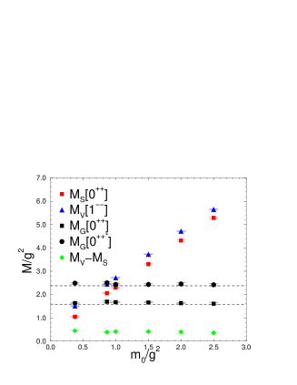
Figure 3: The lowest states in 3d scalar QCD [17]. $M_{G}$ denotes scalar glueballs, $M_{S,V}$ scalar and vector mesons. The gauge coupling is 3d.

Moreover, integrating the scalars out analytically, one obtains for the ratio of correlators

$$\frac{\langle V({\bf x},0)V({\bf x},t)\rangle_{c}}{\langle S({\bf x},0)S({\bf x},t)\rangle_{c}}\sim\frac{\int DA\;{\rm Tr\,}\left(D_{i}({\bf x},0)U_{0}(0,t)D_{i}({\bf x},t)U^{\dagger}_{0}(0,t)\right){\rm e}^{-S_{YM}}}{\int DA\;{\rm Tr\,}\left(U_{0}(0,t)U^{\dagger}_{0}(0,t)\right){\rm e}^{-S_{YM}}}.$$ (7)

In temporal gauge this reduces to the gluon propagator again. In other words, the mass difference $M_{V}-M_{S}$ in the static limit should be equivalent to the pole mass of the gluon. (Similarly, a correlation length for thermal electric gluons was recently extracted from a ratio of singlet correlators [22].)

Numerical results for 2+1 dimensional SU(2) are shown in Figure 3. With increasing scalar mass, the measured glueball states $M_{G}$ attain their pure gauge values indicated by the dashed lines. The scalar bound states move out of the spectrum, with $M_{V}-M_{S}$ approximately constant. At the largest scalar mass one finds $m_{A}=0.37(6)g_{3}^{2}$, or $M_{G}/m_{A}\approx 4.2$.

Rather than approaching the static limit numerically, one may also compute it directly, beginning from the right hand side of Eq. (7). The numerator is a continuum version of the lattice operator Eq. (4), the difference being that the time-like strings are not zero momentum projected. In discretizing the covariant derivative, the non-local functionals should be avoided. This is achieved by observing that the exponential decay of a correlator is entirely determined by the Hamiltonian and the quantum numbers of the operators used. Instead of discretizing the covariant derivative, one can then equally well employ a local higher dimension operator sharing the same quantum numbers, such as $(D_{j}F_{ij}(x))^{a}$. The discretized version of the latter is simply the adjoint part of a linear combination of plaquettes, and hence a local operator. The denominator, on the other hand, consists of a Wilson line running back and forth, i.e. an adjoint Wilson line, which has the same exponential decay as a field strength correlator [23]. The discretized version of Eq. (7) is then simply given by a ratio of gluelump correlators with the appropriate quantum numbers,

$$\frac{\left\langle{\rm Tr\,}\left(D_{i}F_{ij}({\bf x},0)U_{0}(0,t)D_{i}F_{ij}({\bf x},t)U_{0}^{\dagger}(0,t)\right)\right\rangle}{\left\langle{\rm Tr\,}\left(F_{ij}({\bf x},0)U_{0}(0,t)F_{ij}({\bf x},t)U_{0}^{\dagger}(0,t)\right)\right\rangle},$$ (8)

and its asymptotic exponential decay is the mass difference of the corresponding gluelump masses, in which the divergent self-energies of the Wilson lines cancel. (Note that, had we coupled the gluon to one adjoint source field instead of two fundamental, we would have obtained the same static limit.) The calculation performed in [17] and extrapolated to the continuum gives as the final result

$$m_{A}=0.360(19)g_{3}^{2}.$$ (9)

Note the agreement with the result obtained by using heavy scalar fields.

6 The magnetic mass

In the framework of the 4d thermal field theory, the 3d gluon mass appears at asymptotic temperatures as the magnetic mass for hot SU(2) gauge theory, which then is $m_{A}=0.36(2)g^{2}T$. It is now interesting to compare with gauge invariant resummation schemes of perturbation theory and a Hamiltonian strong coupling analysis, all done in the 3d gauge theory, which have been used in the past to compute the pole of the propagator. As the Table shows, the leading order results of all these calculations get within 20% of the right answer, and the two-loop calculation [24] in one of the schemes [9] even suggests reasonable convergence.

	Ref.		$m_{A}/g_{3}^{2}$
1-loop gap eq.	[10]		0.38
	[9, 11]		0.28
	[12]		0.25
2-loop gap eq. for [9]	[24]		0.34
Hamiltonian strong coupl.	[25]		0.32

Figure 4: Volume dependence of the sphaleron rate, which picks up at $2l_{mag}$ (the 2 is for the periodic boundary conditions) [26].

For non-perturbative evidence for the role of this quantity in non-abelian plasmas, recall Guy Moore’s contribution to SEWM 2000 [26], in which he showed the finite size scaling behavior of the sphaleron rate in the hot SU(2) pure gauge theory. This is obtained by simulations of the effective theory for the soft modes $\sim g^{2}T$ and shown in Figure 4. A quantity is typically afflicted by finite size effets as long as the correlation length corresponding to the relevant modes does not fit into the simulated box, $L\leq\xi$, and begins to approach its infinite volume limit once $L>\xi$. The sphaleron rate displays a rather clear signal for this, and the correlation length one estimates from the plot is fully compatible with $m_{A}^{-1}$, while being completely at odds with $M_{G}^{-1}$.

7 Conclusions

By constructing a non-local lattice operator whose correlation function is amenable to the transfer matrix formalism, I have shown that a non-perturbative, gauge invariant mass scale is associated with the gluon field, representing the smallest eigenvalue of the Kogut-Susskind Hamiltonian in the presence of external charges. In momentum space it corresponds to a pole in the propagator in all unique gauges that are local in time. The eigenvalue can be related to some particular level splittings of static mesons. I have calculated this quantity for the 2+1 dimensional SU(2) pure gauge theory, and found it to be roughly a quarter of the glueball mass. This implies a magnetic mass for the hot SU(2) gauge theory, whose inverse constitutes the largest correlation length of the system at asymptotic temperatures. Of course, close to $T_{c}$ the increase of $g^{2}(T)$ may lead to level crossings with electric modes and change this picture, and so will the addition of light fermion flavors. But non-perturbatively dressed partons are theoretically accessible and, as the sphaleron example shows, might be the relevant degrees of freedom for certain aspects of plasma dynamics.

References

- [1] F. Karsch, AIP Conf. Proc. 602 (2001) 323, hep-lat/0109017.
- [2] A. Hart et al., Nucl. Phys. B 586 (2000) 443; A. Hart and O. Philipsen, Nucl. Phys. B 572 (2000) 243; M. Laine and O. Philipsen, Phys. Lett. B 459 (1999) 259.
- [3] M. Laine, these proceedings; K. Kajantie et al., hep-ph/0211321.
- [4] P. Ginsparg, Nucl. Phys. B 170 (1980) 388; T. Appelquist and R.D. Pisarski, Phys. Rev. D 23 (1981) 2305.
- [5] A. D. Linde, Phys. Lett. B 96, 289 (1980); D. J. Gross, R. D. Pisarski and L. G. Yaffe, Rev. Mod. Phys. 53, 43 (1981).
- [6] A. S. Kronfeld, Phys. Rev. D 58, 051501 (1998).
- [7] R. Kobes et al., Phys. Rev. Lett. 64, 2992 (1990); Nucl. Phys. B 355, 1 (1991).
- [8] A. K. Rebhan, Phys. Rev. D 48 (1993) 3967; E. Braaten and A. Nieto, Phys. Rev. Lett. 73 (1994) 2402.
- [9] W. Buchmüller and O. Philipsen, Nucl. Phys. B 443, 47 (1995); Phys. Lett. B 354 (1995) 403; Phys. Lett. B 397 (1997) 112.
- [10] G. Alexanian and V. P. Nair, Phys. Lett. B 352, 435 (1995).
- [11] R. Jackiw and S. Pi, Phys. Lett. B 403, 297 (1997).
- [12] J. M. Cornwall, Phys. Rev. D 57, 3694 (1998);
- [13] V. N. Gribov, Nucl. Phys. B 139, 1 (1978); P. van Baal, hep-th/9711070.
- [14] P. Arnold and L. G. Yaffe, Phys. Rev. D 52 (1995) 7208.
- [15] For a review comparing all definitions, see O. Philipsen, hep-ph/0010327.
- [16] O. Philipsen, Phys. Lett. B 521 (2001) 273.
- [17] O. Philipsen, Nucl. Phys. B 628 (2002) 167.
- [18] J. Vink and U. Wiese, Phys. Lett. B 289 (1992) 122. G. Mack et al., hep-lat/9205013; J. Vink, Phys. Rev. D 51 (1995) 1292.
- [19] M. Creutz, Phys. Rev. D 15, 1128 (1977); M. Lüscher, Commun. Math. Phys. 54, 283 (1977).
- [20] J. Kogut and L. Susskind, Phys. Rev. D 11, 395 (1975).
- [21] O. Philipsen et al., Nucl. Phys. B 469 (1996) 445; Nucl. Phys. B 528 (1998) 379.
- [22] S. Datta and S. Gupta, hep-lat/0208001.
- [23] C. Michael, Nucl. Phys. B 259 (1985) 58; I. H. Jorysz and C. Michael, Nucl. Phys. B 302 (1988) 448.
- [24] F. Eberlein, Phys. Lett. B 439 (1998) 130;
- [25] D. Karabali, C. Kim and V. P. Nair, Nucl. Phys. B 524 (1998) 661.
- [26] G. D. Moore, hep-ph/0009161 and references therein.