Non-factorizable effects in $B\,-\,\overline{B}$ mixing

Abstract

We study the $B$-parameter (“bag factor”) for $B-\overline{B}$ mixing within a recently developed heavy-light chiral quark model. Non-factorizable contributions in terms of gluon condensates and chiral corrections are calculated. In addition, we also consider $1/m_{Q}$ corrections within heavy quark effective field theory. Perturbative QCD effects below $\mu=m_{b}$ known from other work are also included. Considering two sets of input parameters, we find that the renormalization invariant $B$-parameter is $\hat{B}=1.51\pm 0.09$ for $B_{d}$ and $\hat{B}=1.40\pm 0.16$ for $B_{s}$.

I Introduction

Studies of the neutral $K$-meson system have played a major role in modern particle physics KKbar . Because of weak interactions, a neutral $K$ meson may be transferred to a neutral $\overline{K}$ meson. This process, known as $K-\overline{K}$ mixing, determines both the mass-difference between the physical neutral states $K_{L}$ and $K_{S}$ and the dominating CP-violating effect in neutral $K$-meson decays to pions (the $\varepsilon$-effect). The neutral $B$-meson system has rather similar properties as the neutral $K$-system. The difference when going to $B\,-\,\overline{B}$ mixing is the importance of other KM quark mixing factors and other mass scales, in particular the $B$-mesons are about ten times heavier than the $K$-mesons.

In general, non-leptonic processes may be described by an effective Lagrangian which is a linear combination of quark operators. The (Wilson) coefficients of the operators can be calculated in perturbation theory combined with the renormalization group equations weak . At quark level, the leading order diagrams for $B-\overline{B}$ mixing are given by the so called box diagram. This diagram has double $W$- exchange between two quark lines, and generates an effective Lagrangian(Hamiltonian) for the quark transition $\bar{b}d\rightarrow\bar{d}b$. This Lagrangian has (for all practical purposes) only one operator times a Wilson coefficient containing the effects of the virtual ($u,c,t$) quarks running in the loop. This Wilson coefficient has also been corrected for perturbative QCD effects within the renormalization group equations. Such calculations has been performed to next to leading order. For $B_{s}-\overline{B_{s}}$ mixing one considers the corresponding $\bar{b}s\rightarrow\bar{s}b$ transition.

The difficult part is to calculate the matrix elements of the quark operators between the mesonic states, which is a non-perturbative issue. This has been done by lattice simulations latt ; Mar-latt or by quark models Mel . The hadronic matrix element is, as for $K-\overline{K}$ mixing, parameterized through the so called $B$- (“bag”-) parameter which is by construction equal to one in the naive limit when vacuum states are inserted between the quark currents in the $B-\overline{B}$ mixing operator.

In a previous paper BEFL , $K-\overline{K}$ mixing was calculated within a chiral quark model ($\chi$QM) combined with chiral perturbation theory. Within the $\chi$QM, non-factorizable contributions can also be calculated in terms of gluon condensates. The purpose of this paper is to perform a similar analysis for $B\,-\,\overline{B}$ mixing. We are using a recently developed heavy-light chiral quark model (HL$\chi$QM) ahjoe , where non-factorizable effects can be incorporated by means of gluon condensates and chiral loops.

II $B\,-\,\overline{B}$ mixing and heavy quark effective theory

At quark level, the standard effective Lagrangian describing $B\,-\,\overline{B}$ mixing is weak :

$${\cal L}_{eff}^{\Delta B=2} = -\,\frac{G_{F}^{2}}{4\pi^{2}}M_{W}^{2}\left(V_{tb}^{*}V_{tq}\right)^{2}\,S_{0}\left(x_{t}\right)\,\eta_{B}\,b(\mu)\;Q(\Delta B=2)\;,$$ (1)

where $G_{F}$ is Fermi’s coupling constant, the $V$’s are KM factors KM (for which $q=d$ or $s$ for $B_{d}$ and $B_{s}$ respectively) and $S_{0}$ is the Inami-Lim function inami due to short distance electroweak loop effects for the box diagram:

$$S_{0}(x)=\frac{4x-11x^{2}+x^{3}}{4(1-x)^{2}}-\frac{3x^{3}\,\text{Log}\,x}{2(1-x)^{3}}\,.$$ (2)

In our case, $x=x_{t}\equiv m_{t}^{2}/M_{W}^{2}$, where $m_{t}$ is the top quark mass. Because of its large mass, the top quark gives the dominant contribution. Also the $u$ and $c$ quarks are running in the loop, but these contributions are KM suppressed. The quantity $Q(\Delta B=2)$ is a four quark operator :

$$Q(\Delta B=2)=\overline{q_{L}}\,\gamma^{\alpha}\,b_{L}\;\overline{q_{L}}\,\gamma_{\alpha}\,b_{L}\;,$$ (3)

where $q_{L}$ $(b_{L})$ is the left-handed projection of the $q$ $(b)$-quark field. The quantities $\eta_{B}$ and $b(\mu)$ are calculated in perturbative quantum chromodynamics (QCD). At the next to leading order (NLO) analysis it is found that $\eta_{B}=0.55\pm 0.01\,$ weak . Furthermore, for a renormalization point $\mu$ in perturbative QCD equal to or below $m_{b}$,

$$b(\mu)\,=\,\left[\alpha_{s}(\mu)\right]^{-6/23}\left[1+\frac{\alpha_{s}(\mu)}{4\pi}J_{5}\right]\;,$$ (4)

where $J_{5}$ = 1.63 in the naive dimension regularization scheme (NDR). At $\mu~{}=~{}m_{b}$ $(=4.8~{}\text{GeV})$ one has $b(m_{b})\simeq 1.56$.

The matrix element of the operator $Q(\Delta B=2)$ between the meson states is parameterized by the bag parameter $B_{B_{q}}$ :

$${\langle}B|Q(\Delta B=2)|\overline{B}{\rangle}{\,\equiv\,}\frac{2}{3}f_{B}^{2}M_{B}^{2}B_{B_{q}}(\mu)\;\,.$$ (5)

By definition, $B_{B_{q}}=1$ within naive factorization, also named vacuum saturation approach (VSA). This means to insert a vacuum state between the two heavy-light currents in the operator $Q(\Delta B=2)$, and use the matrix elements defining the decay constant $f_{B}$:

$${\langle}0|\overline{q_{L}}\,\gamma^{\mu}\,b|\overline{B}(p){\rangle}=\frac{i}{2}\,f_{B}\,p^{\mu}\;\qquad\text{and}\qquad{\langle}B(p)|\overline{q_{L}}\,\gamma^{\mu}\,b|0{\rangle}=-\frac{i}{2}\,f_{B}\,p^{\mu}\;.$$ (6)

One may combine naive factorization with the large $N_{c}$ expansion, where $N_{c}$ is the number of colours. Then one finds $B_{B_{q}}=3(1+1/N_{c})/4$, giving $B_{B_{q}}=3/4$ in the (naive) large $N_{c}$ limit. We will see later that there are important non-factorizable contributions of order $1/N_{c}$. In general, the matrix elements of the operator $Q(\Delta B=2)$ are dependent on the renormalization scale $\mu$, and thereby $B_{B_{q}}$ depends on $\mu$. As for $K-\overline{K}$ mixing, one defines a renormalization scale independent quantity

$$\hat{B}_{B_{q}}\equiv b(\mu)B_{B_{q}}(\mu)\;.$$ (7)

Within lattice gauge theory, values for $\hat{B}_{B_{q}}$ between 1.3 and 1.5 are obtained latt ; Mar-latt .

The mass difference between the weak eigenstates ($B_{H}$ and $B_{L}$) are related to the bag parameter in the following way for $B_{q}=B_{d},B_{s}$:

$$\Delta m_{q}=\frac{G_{F}^{2}}{6\pi^{2}}m_{B_{q}}f_{B_{q}}^{2}\hat{B}_{B_{q}}\eta_{B}M_{W}^{2}\,S_{0}\left(m_{t}^{2}/M_{W}^{2}\right)\,|V_{tq}^{*}V_{tb}|^{2}\;.$$ (8)

In order to extract the KM matrix elements it is crucial to have a precise knowledge of the bag parameter $\hat{B}_{B_{q}}$, and the weak decay constant $f_{B_{q}}$.

The $b$ -quark is heavy compared to the typical hadronic scale of order 1 GeV, where confinement and chiral symmetry breaking effects are essential. Perturbative effects below the $b$-quark scale may then be calculated down to 1 GeV by means of heavy quark effective theory (HQEFT. See neu for a review). Thus HQEFT also allows us to evolve the matrix element (3) from $\mu=m_{b}$ down to 1 GeV.

HQEFT is a systematic expansion in $1/m_{b}$. The heavy quark field $b(x)$ is replaced by a “reduced” field, $Q_{v}^{(+)}(x)$ or $Q_{v}^{(-)}(x)$, which is related to the full field the in following way:

$$Q_{v}^{(\pm)}(x)=P_{\pm}e^{\mp im_{b}v\cdot x}b(x)\,,$$ (9)

where $P_{\pm}$ are projecting operators $P_{\pm}=(1\pm\gamma\cdot v)/2$. The reduced field $Q_{v}^{(+)}$ can only annihilate heavy quarks. In order to describe heavy anti-quarks one has to use $Q_{v}^{(-)}$. In other words, $Q^{(+)}_{v}(Q_{v}^{(-)})$ annihilates (creates) a heavy quark (anti-quark) with velocity $v$. The Lagrangian for heavy quarks is ($Q_{v}=Q_{v}^{(\pm)}$):

$${\cal L}_{\text{HQEFT}}=\pm\overline{Q_{v}}\,iv\cdot D\,Q_{v}+\frac{1}{2m_{Q}}\overline{Q_{v}}\,\left(-C_{M}\frac{g_{s}}{2}\sigma\cdot G\,+\,(iD_{\perp})_{\text{eff}}^{2}\right)\,Q_{v}+{\cal O}(m_{Q}^{-2})\;\,,$$ (10)

where $D_{\mu}$ is the covariant derivative containing the gluon field (eventually also the photon field), and $\sigma\cdot G=\sigma^{\mu\nu}G^{a}_{\mu\nu}t^{a}$, where $\sigma^{\mu\nu}=i[\gamma^{\mu},\gamma^{\nu}]/2$, $G^{a}_{\mu\nu}$ is the gluonic field tensors, and $t^{a}$ are the colour matrices. This chromo-magnetic term has a factor $C_{M}$ which is one at tree level, but slightly modified by perturbative QCD effects below the scale $m_{b}$ . It has been calculated to NLO neub ; grozin1 . Furthermore, $(iD_{\perp})_{\text{eff}}^{2}=C_{D}(iD)^{2}-C_{K}(iv\cdot D)^{2}$. At tree level, $C_{D}=C_{K}=1$. Here, $C_{D}$ is not modified by perturbative QCD, while $C_{K}$ is different from one due to perturbative QCD corrections GriFa . In our case, $m_{Q}=m_{b}$ is the heavy quark mass.

Running from $\mu=m_{b}$ down to $\mu=\Lambda_{\chi}=1\,$ GeV, there will appear more operators. Some stem from the heavy quark expansion itself and some are generated by perturbative QCD effects. The $\Delta B=2$ operator in equation (3) for $\Lambda_{\chi}<\mu<m_{b}$ can be written gimenez1 ; mannel ; gimenez2 :

$$Q(\Delta B=2)= \,C_{1}(\mu)\;Q_{1}+C_{2}(\mu)\;Q_{2}+\frac{1}{m_{b}}\left(\sum_{i}^{6}a_{i}(\mu)S_{i}(\mu)\right.$$ (11)

$$\left.+\sum_{i}^{3}\,h_{i}(\mu)X_{i}(\mu)\right)\,+{\cal O}(1/m_{b}^{2})\;\,.$$

The operator $Q_{1}$ is $Q(\Delta B=2)$ for $b$ replaced by $Q_{v}^{(\pm)}$, while $Q_{2}$ is generated within perturbative QCD for $\mu<m_{b}$. The operators $S_{i}$ and $X_{i}$ are taking care of $1/m_{b}$ corrections. The quantities $C_{1},C_{2},a_{i},h_{i}$ are Wilson coefficients. ($C_{1}=1+{\cal O}(\alpha_{s})$ and $C_{2}=0+{\cal O}(\alpha_{s}))$. The explicit expressions for the operators are

$$Q_{1} =2\;\overline{q_{L}}\,\gamma^{\mu}\,Q^{(+)}_{v}\;\;\overline{q_{L}}\,\gamma_{\mu}\,Q^{(-)}_{v}\,\;,$$ (12)

$$Q_{2} =2\;\overline{q_{L}}\,v^{\mu}\,Q^{(+)}_{v}\;\;\overline{q_{L}}\,v_{\mu}\,Q^{(-)}_{v}\;\,,$$ (14)

$$X_{1} =2\;\overline{q_{L}}\,iD\hskip-5.0pt/\,Q^{(+)}_{v}\;\;\overline{q_{L}}\,Q^{(-)}_{v}\,+\,2\;\overline{q_{L}}\,iD^{\mu}\,Q^{(+)}_{v}\;\;\overline{q_{L}}\,\gamma_{\mu}\,Q^{(-)}_{v}\,$$

$$-2\,i\,\varepsilon_{\lambda\mu\nu\rho}\,v^{\lambda}\,\overline{q_{L}}\,iD^{\mu}\gamma^{\nu}\,Q^{(+)}_{v}\;\;\overline{q_{L}}\,\gamma^{\rho}\,Q^{(-)}_{v}$$

$$+\,2\;\overline{q_{L}}\,Q^{(+)}_{v}\;\;\overline{q_{L}}\,iD\hskip-5.0pt/\,Q^{(-)}_{v}\,+\,2\;\overline{q_{L}}\,\gamma_{\mu}\,Q^{(+)}_{v}\;\;\overline{q_{L}}\,iD^{\mu}\,Q^{(-)}_{v}$$

$$-i2\,\,\varepsilon_{\lambda\mu\nu\rho}\,v^{\lambda}\,\overline{q_{L}}\,\gamma^{\nu}\,Q^{(+)}_{v}\;\;\overline{q_{L}}\,iD^{\mu}\gamma^{\rho}\,Q^{(-)}_{v}\;\,,$$

$$X_{2} =8\,\left[iv\cdot\partial(\overline{q_{L}}\,Q^{(+)}_{v})\right]\overline{q_{L}}\,Q^{(-)}_{v}+\,2\,\left[iv\cdot\partial(\overline{q_{L}}\gamma_{\mu}\,Q^{(+)}_{v})\right]\overline{q_{L}}\,\gamma^{\mu}\,Q^{(-)}_{v}\,,$$ (15)

$$X_{3} =4\,\left[iv\cdot\partial(\overline{q_{L}}\gamma_{\mu}\,Q^{(+)}_{v})\right]\overline{q_{L}}\,\gamma^{\mu}\,Q^{(-)}_{v}\;\,.$$ (16)

The operators $S_{i}$ are nonlocal and is a combination of the leading order operators $Q_{1,2}$ and a term of order $1/m_{Q}$ from the effective Lagrangian (10):

$$\frac{S_{1}}{m_{b}} = i\int dy^{4}T\{Q_{1}(0),O_{K}(y)\}\;,$$

$$\frac{S_{2}}{m_{b}} = i\int d^{4}yT\{Q_{2}(0),O_{K}(y)\}\;,$$

$$\frac{S_{3}}{m_{b}} = i\int d^{4}yT\{Q_{1}(0),O_{M}(y)\}\;,$$

$$\frac{S_{4}}{m_{b}} = i\int d^{4}yT\{Q_{2}(0),O_{M}(y)\}\;,$$ (17)

where

$$O_{K}\,{\,\equiv\,} \,\frac{1}{2m_{b}}\left(\overline{Q^{(+)}_{v}}\,(iD_{\perp})_{\text{eff}}^{2}\,Q^{(+)}_{v}+\overline{Q^{(-)}_{v}}\,(iD_{\perp})_{\text{eff}}^{2}\,Q^{(-)}_{v}\right)\;\,,$$ (18)

$$O_{M}\,{\,\equiv\,} \,-\frac{g_{s}}{4m_{b}}\left(\overline{Q^{(+)}_{v}}\,\sigma\cdot G\,Q^{(+)}_{v}+\overline{Q^{(-)}_{v}}\,\sigma\cdot G\,Q^{(-)}_{v}\right)\;\,,$$

are the kinetic and magnetic operators of eq. (10). There are no mixing between the local operators and the non-local operators, since the local operators do not need the non-local ones as counter-terms. The Wilson coefficients $a_{i}$ will then be the product of $C_{1,2}$ and $C_{M,K}$. The Wilson coefficients $C_{1}$ and $C_{2}$ have been calculated to NLO gimenez1 ; gimenez2 and for $\mu=\Lambda_{\chi}$, $C_{1}(\Lambda_{\chi})=1.22$ and $C_{2}(\Lambda_{\chi})=-0.15$. The coefficients $h_{1,2,3}$ have been calculated to leading order (LO) in mannel , and the result at $\mu=\Lambda_{\chi}$ is $h_{1}=0.52$, $h_{2}=-0.16$ and $h_{3}=-0.15$.

III The heavy-light chiral quark model

In order to calculate the matrix elements we will use the heavy-light chiral quark model (HL$\chi$QM) recently developed in ahjoe . This is a type of quark loop model chiqm ; barhi ; itCQM ; effr where the quarks couples directly to the mesons at the scale of chiral symmetry breaking $\Lambda_{\chi}$, which we put equal to 1 GeV. What makes our model ahjoe distinct from other similar models is that it incorporates soft gluon effects in terms of the gluon condensate with lowest dimension BEFL ; pider ; epb ; BEF ; EHP . The term in the Lagrangian describing this interaction can be obtained as a mean-field approximation of the (extended) Nambu-Jona-Lasinio model (NJL) bijnes ; effr .

In this section we will give a short presentation of the HL$\chi$QM. In the next section we will use the model ahjoe to calculate non-factorizable soft gluon effects in $B\,-\,\overline{B}$ mixing.

The Lagrangian for the HL$\chi$QM is

$${\cal L}_{\text{HL$\chi$QM}}={\cal L}_{\text{HQEFT}}+{\cal L}_{\chi\text{QM}}+{\cal L}_{\text{Int}}\;\,.$$ (19)

The first term is given in equation (10). The light quark sector is described by the chiral quark model ($\chi$QM), having a standard QCD term and a term describing interactions between quarks and (Goldstone) mesons:

$${\cal L}_{\chi\text{QM}}=\overline{\chi}\left[\gamma^{\mu}(iD_{\mu}+{\cal V}_{\mu}+\gamma_{5}{\cal A}_{\mu})-m\right]\chi-\overline{\chi}\,\widetilde{M_{q}}\,\chi\;,$$ (20)

where $\chi_{L,R}$ are the flavour rotated quark fields given by:

$$\chi_{L}=\xi^{\dagger}q_{L}\quad;\qquad\chi_{R}=\xi q_{R}\quad;\qquad\xi\cdot\xi=\Sigma\;.$$ (21)

where $q^{T}=(u,d,s)$ are the light quark fields. The left- and right-handed projections $q_{L}$ and $q_{R}$ are transforming after $SU(3)_{L}$ and $SU(3)_{R}$ respectively. The quantity $\xi$ is a 3 by 3 matrix containing the (would be) Goldstone octet ($\pi,K,\eta$) :

$$\xi=e^{i\Pi/f}\,\quad\text{where}\,\quad\Pi=\frac{\lambda^{a}}{2}\phi^{a}(x)=\frac{1}{\sqrt{2}}\left[\begin{array}[]{ccc}\frac{\pi^{0}}{\sqrt{2}}+\frac{\eta_{8}}{\sqrt{6}}&\pi^{+}&K^{+}\\ \pi^{-}&-\frac{\pi^{0}}{\sqrt{2}}+\frac{\eta_{8}}{\sqrt{6}}&K^{0}\\ K^{-}&\overline{K^{0}}&-\frac{2}{\sqrt{6}}\eta_{8}\end{array}\right]\;,$$ (22)

where $f$ is the bare pion decay constant. In (20), $m$ is the ($SU(3)$ - invariant) constituent quark mass for light quarks, and $\widetilde{M_{q}}$ contains the current quark mass matrix ${\cal M}_{q}$ and the field $\xi$:

$$\widetilde{M_{q}}{\,\equiv\,}\widetilde{M}_{q}^{V}+\widetilde{M}_{q}^{A}\gamma_{5}\;,\;\;\text{where}$$ (23)

$$\widetilde{M}_{q}^{V}\,{\,\equiv\,}\,\frac{1}{2}(\xi^{\dagger}{\cal M}_{q}^{\dagger}\xi^{\dagger}\;+ \xi{\cal M}_{q}\xi)\quad\text{and}\quad\widetilde{M}_{q}^{A}{\,\equiv\,}-\frac{1}{2}(\xi^{\dagger}{\cal M}_{q}^{\dagger}\xi^{\dagger}-\xi{\cal M}_{q}\xi)\;.$$ (24)

The vector and axial vector fields ${\cal V}_{\mu}$ and ${\cal A}_{\mu}$ in (20) are given by:

$${\cal V}_{\mu}{\,\equiv\,}\frac{i}{2}(\xi^{\dagger}\partial_{\mu}\xi+\xi\partial_{\mu}\xi^{\dagger})\qquad;\qquad{\cal A}_{\mu}{\,\equiv\,}-\frac{i}{2}(\xi^{\dagger}\partial_{\mu}\xi-\xi\partial_{\mu}\xi^{\dagger})\;\,.$$ (25)

Furthermore, the covariant derivative $D_{\mu}$ in (20) contains the soft gluon field forming the gluon condensates. The gluon condensate contributions are calculated by Feynman diagram techniques as in BEFL ; ahjoe ; epb ; BEF . They may also be calculated by means of heat kernel techniques as in pider ; bijnes ; ebert3 .

The interaction between heavy meson fields and heavy quarks are described by the following Lagrangian :

$${\cal L}_{Int}=-G_{H}\,\left[\overline{\chi}_{a}\,\overline{H_{a}^{(\pm)}}\,Q^{(\pm)}_{v}\,+\overline{Q_{v}^{(\pm)}}\,H_{a}^{(\pm)}\,\chi_{a}\right]\,+\,\frac{1}{2G_{3}}Tr\left[\overline{H_{v}^{a}}\,H_{v}^{a}\right]\;\,,$$ (26)

where $G_{H}$ and $G_{3}$ are coupling constants and $H_{a}^{(\pm)}$ is the heavy meson field containing a spin zero and spin one boson:

$$H_{a}^{(\pm)} {\,\equiv\,}P_{\pm}(P_{a\mu}^{(\pm)}\gamma^{\mu}-iP_{5a}^{(\pm)}\gamma_{5})\;\;\;,\;\;\overline{H_{a}^{(\pm)}}{\,\equiv\,}\gamma^{0}(H_{a}^{(\pm)})^{\dagger}\gamma^{0}\;.$$ (27)

The fields $P^{(+)}(P^{(-)})$ annihilates (creates) a heavy meson containing a heavy quark (anti quark) with velocity $v$.

Integrating out the quarks by using (10), (20) and (26), the effective Lagrangian up to ${\cal O}(m_{Q}^{-1})$ can be written as itchpt ; ahjoe :

$${\cal L}=\mp Tr\left[\overline{H^{(\pm)}_{a}}\left(iv\cdot{\cal D}_{ba}-\Delta_{Q}\right)H^{(\pm)}_{b}\right]\,-\,{g_{{\cal A}}}\,Tr\left[\overline{H^{(\pm)}_{a}}H^{(\pm)}_{b}\gamma_{\mu}\gamma_{5}{\cal A}^{\mu}_{ba}\right]\,,$$ (28)

where $i{\cal D}^{\mu}_{ba}=i\delta_{ba}D^{\mu}-{\cal V}^{\mu}_{ba}$. The term proportional to the quark-meson mass difference $\Delta_{Q}=M_{H}-m_{Q}$ in (28) is irrelevant for us due to the reparametrization invariance neu . Also, it does not enter our loop integrals because our heavy meson fields are attached to our quark loops at zero external momentum. (The external momentum includes the piece $v^{\mu}\Delta_{Q}$). As shown in ahjoe , the term $\sim 1/G_{3}$ in (26) is related to $\Delta_{Q}$, and this term is also irrelevant within the present paper.

To obtain (28) from the HL$\chi$QM one encounters divergent loop integrals, which might be quadratic-, linear- and logarithmic divergent. For the kinetic term in (28) we obtain the identification:

$$-iG_{H}^{2}N_{c}\,\left(I_{3/2}+2mI_{2}-i\frac{(3\pi-8)}{384m^{3}N_{c}}{\langle}\frac{\alpha_{s}}{\pi}G^{2}{\rangle}\right)=1\;\,,$$ (29)

where $I_{3/2}$ and $I_{2}$ are the linear and logarithmic divergent integrals respectively, and ${\langle}\frac{\alpha_{s}}{\pi}G^{2}{\rangle}$ is the gluon condensate. To obtain the axial vector term proportional to $g_{\cal A}$, we obtain a similar condition, and combining it with (29), we obtain for the axial vector term

$${g_{{\cal A}}}=1+\frac{4}{3}iG_{H}^{2}N_{c}\left(I_{3/2}-\frac{im}{16\pi}\right)\;\,,$$ (30)

such that the (formally) linear divergent integral $I_{3/2}$ is related to the strong axial coupling ${g_{{\cal A}}}$ (or strictly speaking, its deviation from one). Analogously, within the pure light quark sector (the $\chi$QM), it is well known that the quadratic and logarithmic divergent integrals are related to the quark condensate and the bare decay constant $f$, respectively chiqm ; pider ; epb ; BEF ; ebert3 :

$${\langle}\,\overline{q}q\,{\rangle} =-4imN_{c}I_{1}-\frac{1}{12m}{\langle}\frac{\alpha_{s}}{\pi}G^{2}{\rangle}\;\,,$$ (31)

$$f^{2} =-i4m^{2}N_{c}I_{2}+\frac{1}{24m^{2}}{\langle}\frac{\alpha_{s}}{\pi}G^{2}{\rangle}\;\,.$$ (32)

The divergent integrals $I_{1},\,I_{2}$ and $I_{3/2}$ are listed in appendix A. The effective coupling $G_{H}$ describing the interaction between the quarks and heavy mesons can be expressed in terms of $m$, $f$, $g_{\cal A}$, and the mass splitting between the $1^{-}$ state and $0^{-}$ state. Using (29), (30), (32) one finds a relation between this mass-splitting and the gluon condensate via the chromomagnetic interaction in (10) ahjoe :

$${\langle}\frac{\alpha_{s}}{\pi}G^{2}{\rangle}=\frac{16f^{2}}{\pi\eta}\,\frac{\mu_{G}^{2}}{\rho}\;\,,\qquad G_{H}^{2}=\frac{2m}{f^{2}}\,\rho\;\,,\qquad\eta\,{\,\equiv\,}\,\frac{(\pi+2)}{\pi}C_{M}(\Lambda_{\chi})\;\,,$$ (33)

where

$$\rho\,{\,\equiv\,}\,\frac{(1+3g_{\cal A})+\frac{\mu_{G}^{2}}{\eta\,m^{2}}}{4(1+\frac{N_{c}m^{2}}{8\pi f^{2}})}\;\;\;,\;\;\;\mu_{G}^{2}(H)\,=\,\frac{3}{2}m_{Q}(M_{H^{*}}-M_{H}).$$ (34)

In the limit where only the leading logarithmic integral $I_{2}$ is kept we obtain :

$$g_{\cal A}\rightarrow\,1\;,\qquad\rho\rightarrow\,1\;,\qquad G_{H}\;\rightarrow\;G_{H}^{(0)}\,{\,\equiv\,}\,\frac{\sqrt{2m}}{f}\;\,.$$ (35)

Note that $g_{\cal A}=1$ is the non-relativistic value itchpt . We observe that the mass-splitting between $H$ and $H^{*}$ sets the scale of the gluon condensate. This means that, while in BEF the gluon condensate was fitted to the $K\rightarrow(2\pi)_{I=2}$ amplitude, it is here determined in the strong sector alone (with a slightly lower value than in BEF ).

The $1/m_{Q}$ corrections to the strong Lagrangian have been calculated in ahjoe . They may formally be put into spin dependent renormalization factors. This means that (28) is still valid with the replacement $H^{\text{r}}=H\,(Z_{H})^{-\frac{1}{2}}$, where $Z_{H}$ and the renormalized (effective) coupling $\tilde{g}_{{\cal A}}$ are defined as:

$$Z_{H}^{-1} = 1+\frac{\varepsilon_{1}-2d_{M}\varepsilon_{2}}{m_{Q}}\;\;,$$ (36)

$$\tilde{g}_{{\cal A}} = {g_{{\cal A}}}\left(1-\frac{1}{m_{Q}}(\varepsilon_{1}-2d_{\cal A}\varepsilon_{2})\right)-\frac{1}{m_{Q}}(g_{1}-d_{\cal A}g_{2})\;\,,$$ (37)

where

$$d_{M}=\begin{cases}\,\,\,\,\,3\quad\text{for}\quad 0^{-}\\ -1\quad\text{for}\quad 1^{-}\end{cases}\quad\quad d_{\cal A}=\begin{cases}\,\,\,\,1\quad\text{for}\quad H^{*}H\,\,\,\quad\text{coupling}\\ -1\quad\text{for}\quad H^{*}H^{*}\quad\text{coupling}\end{cases}$$ (38)

and :

$$\varepsilon_{1} = -m+G_{H}^{2}\left(\frac{{\langle}\,\overline{q}q\,{\rangle}}{4m}+f^{2}+\frac{N_{c}m^{2}}{16\pi}+\frac{C_{K}}{16}(\frac{{\langle}\,\overline{q}q\,{\rangle}}{m}-f^{2})\right.$$ (39)

$$\left.\qquad\qquad\quad+\frac{1}{128m^{2}}(C_{K}+8-3\pi){\langle}\frac{\alpha_{s}}{\pi}G^{2}{\rangle}\right)\;,$$

$$g_{1} = \,m-G_{H}^{2}\left(\frac{{\langle}\,\overline{q}q\,{\rangle}}{12m}+\frac{f^{2}}{6}+\frac{N_{c}m^{2}(3\pi+4)}{48\pi}-\frac{C_{K}}{16}(\frac{{\langle}\,\overline{q}q\,{\rangle}}{m}+3f^{2})\right.$$ (40)

$$\left.\qquad\qquad\quad+\frac{1}{64m^{2}}(C_{K}-2\pi){\langle}\frac{\alpha_{s}}{\pi}G^{2}{\rangle}\right)\;,$$

$$g_{2} = \frac{(\pi+4)}{(\pi+2)}\frac{\mu_{G}^{2}}{6m}\;.$$ (41)

IV Bosonizing $Q(\Delta B=2)$

In this section we will discard $1/m_{Q}$ terms. We are then left with the operators $Q_{1,2}$ defined in equation (12) and (14). In order to find the matrix element of $Q_{1,2}\,$, one uses the following relation between the generators of $SU(3)_{c}$ ($i,j,l,n$ are colour indices running from 1 to 3):

$$\delta_{ij}\delta_{ln}=\frac{1}{N_{c}}\delta_{in}\delta_{lj}\;+\;2\;t_{in}^{a}\;t_{lj}^{a}\;,$$ (42)

where $a$ is an index running over the eight gluon charges. This means that by means of a Fierz transformation, the operator $Q_{1}$ in (12) may also be written in the following way :

$$Q_{1}=\frac{2}{N_{c}}\,\overline{q_{L}}\,\gamma^{\mu}\,Q^{(+)}_{v}\,\overline{q_{L}}\,\gamma_{\mu}\,Q^{(-)}_{v}\,+\,4\,\overline{q_{L}}\,t^{a}\,\gamma^{\mu}\,Q^{(+)}_{v}\,\overline{q_{L}}\,t^{a}\,\gamma_{\mu}\,Q^{(-)}_{v}\,,$$ (43)

and similarly for $Q_{2}$.

The first (naive) step to calculate the matrix element of a four quark operator like $Q_{1}$ is by inserting vacuum states between the two currents. This vacuum insertion approach (VSA) corresponds to bosonizing the two currents in $Q_{1}$ and multiply them, as mentioned below eq. (5). For one current, visualized in figure 1, one obtains itchpt ; ahjoe :

$$\overline{q_{L}}\,\gamma^{\mu}\,Q_{v}^{(\pm)}\;\longrightarrow\;\frac{\alpha_{H}}{2}Tr\left[\xi^{\dagger}_{hf}\gamma^{\alpha}L\,H_{h}^{(\pm)}\right]\;,$$ (44)

Using the relations (29) - (32) for the divergent integrals, and also eq. (33), we obtain ahjoe :

$$\alpha_{H}=\frac{G_{H}}{2}\left(-\frac{{\langle}\,\overline{q}q\,{\rangle}}{m}-2f^{2}(1-\frac{1}{\rho})+\frac{(\pi-2)}{16m^{2}}{\langle}\frac{\alpha_{s}}{\pi}G^{2}{\rangle}\right)\;.$$ (45)

This bosonization has to be compared with the matrix elements defining the meson decay constant $f_{B}$ given in eq. (6). In those relations, $b$ is the full quark field. Within HQEFT this matrix element will, below the renormalization scale $\mu=m_{Q}\,(=m_{b})$, be modified in the following way:

$${\langle}0|\overline{q_{L}}\,\Gamma^{\mu}\,Q^{(+)}_{v}|\overline{B}(p){\rangle}=\frac{i}{2}\,f_{B}\,M_{B}\,v^{\mu}\;\quad\text{and}\quad{\langle}B(p)|\overline{q_{L}}\,\Gamma^{\mu}\,Q^{(-)}_{v}|0{\rangle}=-\frac{i}{2}\,f_{B}\,M_{B}\,v^{\mu}\;,$$ (46)

where neu

$$\Gamma^{\mu}\,{\,\equiv\,}\,C_{\gamma}(\mu)\,\gamma^{\mu}\,+\,C_{v}(\mu)\,v^{\mu}\;.$$ (47)

The coefficients $C_{\gamma,v}(\mu)$ are determined by QCD renormalization for $\mu<m_{Q}$. They have been calculated to NLO and the result is the same in $MS$ and $\overline{MS}$ scheme Cgamma . In HL$\chi$QM the decay constant $f_{B}$ can be calculated and the result is ahjoe :

$$\alpha_{H}=\frac{f_{B}\sqrt{M_{B}}}{C_{\gamma}(\mu)+C_{v}(\mu)}=\frac{f_{B^{*}}\sqrt{M_{B^{*}}}}{C_{\gamma}(\mu)}\;\;.$$ (48)

Figure 1: Diagrams for bosonization of the left handed quark current

The second matrix element in (43) is genuinely non-factorizable, and we have to go beyond the VSA. However, in the approximation where only the lowest gluon condensate is taken into account, the last term in (43) can be written in a quasi-factorizable way by bosonizating the heavy-light coloured current with an extra colour matrix $t^{a}$ inserted and with an extra gluon emitted as shown in figure 2. Calculation of this diagram is straightforward when using the light quark propagator with just one soft gluon emitted :

$$S_{G}(k){\,\equiv\,}\frac{g_{s}}{4}G^{b}_{\alpha\beta}t^{b}\left[\sigma^{\alpha\beta}(\gamma\cdot k+m)+(\gamma\cdot k+m)\sigma^{\alpha\beta}\right](k^{2}-m^{2})^{-2}\;\;.$$ (49)

Figure 2: Nonfactorizable contribution, $\Gamma{\,\equiv\,}t^{a}\,\gamma^{\mu}\,L$

The part of the diagram to the left in figure 2 then gives the bosonized coloured current:

$$\left(\overline{q_{L}}t^{a}\,\gamma^{\alpha}Q_{v}^{(\pm)}\right)_{1G}\;\longrightarrow\;-\frac{G_{H}g_{s}}{8}\,G_{\mu\nu}^{a}\;Tr\left[\xi^{\dagger}\gamma^{\alpha}L\,H^{(\pm)}\left(\pm i\,I_{2}\left\{\sigma^{\mu\nu},\gamma\cdot v\right\}+\,\frac{1}{8\pi}\sigma^{\mu\nu}\right)\right]\;,$$ (50)

where $I_{2}$ is to be identified with $f^{2}$ by the use of equation (32). The result for the right part of the diagram with $\bar{B}$ replaced by $B$ is obtained by just changing the sign of $v$ and letting ${P_{5}^{(+)}}\rightarrow{P_{5}^{(-)}}$ (remembering that ${P_{5}^{(-)}}$ creates a meson with a heavy anti quark). Multiplying the coloured currents, we obtain for the non-factorizable part of $Q_{1}$ and $Q_{2}$ to first order in the gluon condensate :

$$C_{1}\,\overline{q_{L}}t^{a}\,\gamma^{\mu}Q^{(+)}_{v}\;\overline{q_{L}}t^{a}\,\gamma_{\mu}\,Q^{(-)}_{v}+C_{2}\,\overline{q_{L}}t^{a}\,v^{\mu}Q^{(+)}_{v}\;\overline{q_{L}}t^{a}\,v_{\mu}\,Q^{(-)}_{v}$$

$$\rightarrow\;-\frac{\beta_{B}}{4}{\langle}\frac{\alpha_{s}}{\pi}G^{2}{\rangle}\left(C_{1}P_{5i}^{(-)}\Sigma_{ii}^{\dagger}P_{5i}^{(+)}\,+(C_{1}-\frac{1}{3}C_{2})\,P_{i}^{(-)\mu}\Sigma_{ii}^{\dagger}P^{(+)}_{i\mu}\right)\;\,,$$ (51)

where

$$\beta_{B}{\,\equiv\,}\frac{G_{H}^{2}}{128}\left\{1+\frac{4\pi}{N_{c}}\left(\frac{f}{m}\right)^{2}+\frac{8\pi^{2}}{N_{c}^{2}}\left(\frac{f}{m}\right)^{4}\right\}\;\,,$$ (52)

and $\Sigma=\xi^{2}$, where $\xi$ is given in Eq. (22). Note there is no sum over $i$, $i=2,3$ for $q=d,s$ respectively.

The Lagrangian in equation (20) contains couplings involving the the current mass term and the chiral quark fields. This makes it possible to calculate the counter-terms needed in order to keep the chiral Lagrangian finite after the inclusion of chiral loops. The counter-term for the factorizable part of the amplitude has been considered in ahjoe when calculating $f_{B}$. In the case of the non-factorizable part of the amplitude, we need to consider similar diagrams as those shown in figure 2, with mass insertion like in figure 3, where mass insertion is indicated by a cross on the light quark line. The bosonized current with mass insertion is

Figure 3: Mass insertion in the nonfactorizable part of the current

$$\left(\overline{q_{L}}t^{a}\,\gamma^{\alpha}Q_{v}^{(\pm)}\right)_{1G,m_{q}}\;\longrightarrow\;\frac{G_{H}g_{s}}{32m\pi^{2}}\,{\varepsilon}^{\alpha\beta\mu\rho}(\pm v_{\alpha})G_{\mu\rho}^{a}\;Tr\left[\xi^{\dagger}\gamma^{\alpha}L\,H_{a}^{(\pm)}\left(\widetilde{M}_{q}^{V}\right)_{aq}\gamma_{\beta}\gamma_{5}\right]\;\,.$$ (53)

This result can also be obtained by simply differentiating the right hand side of equation (50) with respect to $m$.

The bosonized version of the $Q(\Delta B=2)$ operator can then be split in a pseudo scalar and a vector part:

$$Q(\Delta B=2)_{\text{Bos.}}\,=A_{P}\,P_{5i}^{(-)}\Sigma_{ii}^{\dagger}P_{5i}^{(+)}\,+\,A_{V}\,P_{i}^{(-)\mu}\Sigma_{ii}^{\dagger}P^{(+)}_{i\mu}\,\text{, where : }$$

$$A_{P}=\frac{1}{2}(1+\frac{1}{N_{c}})(C_{1}-C_{2})\alpha_{H}^{2}\left(1+2\frac{\omega_{1}}{\alpha_{H}}m_{q}\right)-C_{1}{\langle}\frac{\alpha_{s}}{\pi}G^{2}{\rangle}\left(\beta_{B}+\omega_{\beta}m_{q}\right)\;,$$ (54)

$$A_{V}=\frac{1}{2}(1+\frac{1}{N_{c}})C_{1}\alpha_{H}^{2}\left(1+2\frac{\omega_{1}}{\alpha_{H}}m_{q}\right)-{\langle}\frac{\alpha_{s}}{\pi}G^{2}{\rangle}\left((C_{1}-\frac{C_{2}}{3})\beta_{B}+C_{1}\omega_{\beta}m_{q}\right)\;.$$

The quantity $\omega_{\beta}$ is the counter-term obtained from (53), and $\omega_{1}$ is a counter-term for $f_{B_{s}}$ found in ahjoe :

$$\omega_{\beta} =\frac{G_{H}^{2}}{64\pi m}\left\{1+\frac{4\pi f^{2}}{N_{c}m^{2}}\right\}\;,$$ (55)

$$\omega_{1} =\frac{(1-3{g_{{\cal A}}})}{G_{H}}-\frac{(9\pi-16)G_{H}}{192m^{3}}{\langle}\frac{\alpha_{s}}{\pi}G^{2}{\rangle}\;.$$ (56)

For the current quark mass entering (54) we will use

$$m_{d}=-m_{\pi}^{2}f^{2}/{\langle}\,\overline{q}q\,{\rangle}\;\,,\;\text{and}\;\,m_{s}=-m_{K}^{2}f^{2}/{\langle}\,\overline{q}q\,{\rangle}\;\,.$$ (57)

The term including the vector fields $P_{\mu}$ are needed in order to calculate chiral corrections where $B^{*}$ are included. From equation the equations (5), (7) and (54) the renormalization invariant bag parameter can be extracted. Anticipating the results of the two next sections, it can be written in the form:

$$\hat{B}_{B_{q}}=\frac{3}{4}\,\widetilde{b}\left[1+\frac{1}{N_{c}}\left(1-\delta_{G}^{B}(1+\frac{\tau_{\chi}^{G}}{32\pi^{2}f^{2}})\right)+\frac{\tau_{b}}{m_{b}}+\left(1+\frac{1}{N_{c}}\right)\frac{\tau_{\chi}}{32\pi^{2}f^{2}}\right]\;\,,$$ (58)

where

$$\widetilde{b}\;=\;b(m_{b})\,\left[\frac{C_{1}-C_{2}}{(C_{\gamma}+C_{v})^{2}}\right]_{\mu=\Lambda_{\chi}}\;.$$ (59)

We find from (54) the parameter due to genuine non-factorizable effects:

$$\delta_{G}^{B}\,=\,N_{c}{\langle}\frac{\alpha_{s}}{\pi}G^{2}{\rangle}\frac{\beta_{B}}{\alpha_{H}^{2}}\,\left[\frac{2C_{1}}{C_{1}-C_{2}}\right]_{\mu=\Lambda_{\chi}}\;\,.$$ (60)

Note that this parameter is formally of order $(N_{c})^{0}$ and is positive, which means that this non-factorizable contribution reduces the value of $\hat{B}$ according to (58). Thus we are qualitatively in agreement with Mel , where a negative contribution to the bag factor from gluon condensate effects is found.

Using the relation between $\alpha_{H}$ and $f_{B}$ in Eq. (48) and the expression value for $G_{H}$ in equation (33), we may also write :

$$\delta_{G}^{B}\,=\,\frac{N_{c}{\langle}\frac{\alpha_{s}}{\pi}G^{2}{\rangle}}{32\pi^{2}f^{2}f_{B}^{2}}\,\frac{m}{M_{B}}\,\rho\,\left\{1+\frac{4\pi}{N_{c}}\left(\frac{f}{m}\right)^{2}+\frac{8\pi^{2}}{N_{c}^{2}}\left(\frac{f}{m}\right)^{4}\right\}\,\left[\frac{C_{1}}{C_{1}-C_{2}}\right]_{\mu=\Lambda_{\chi}}\;\ .$$ (61)

Numerically, $f$ and $f_{B}$ are of the same order of magnitude, and $\delta_{G}^{B}$ is therefore suppressed like $m/M_{B}$ compared to the corresponding quantity

$$\delta_{G}^{K}\,=\,N_{c}\frac{{\langle}\frac{\alpha_{s}}{\pi}G^{2}{\rangle}}{32\pi^{2}f^{4}}\;,$$ (62)

for $K-\overline{K}$ mixing. However, one should note that $f_{B}$ scales as $1/\sqrt{M_{B}}$ within HQEFT, and therefore $\delta_{G}^{B}$ is still formally of order $(m_{b})^{0}$.

The formula (58) is a generalization of a similar formula found for $K-\overline{K}$ mixing BEFL . The quantities $\tau_{b}$ and $\tau_{\chi}^{G}$ will be calculated in the next sections, while $\tau_{\chi}$ is known from previous work GrinWise . More specific, the quantity $\tau_{b}$, to be calculated in the next section, has dimension $(mass)^{1}$ and depend on hadronic parameters calculated within the HL$\chi$QM. Similarly, the quantity $\tau_{\chi}$ contains the chiral corrections to the bosonized versions of $Q_{1,2}$ to be presented in section VI. The quantity $\tau^{G}_{\chi}$ contains the chiral corrections proportional to ${\langle}\frac{\alpha_{s}}{\pi}G^{2}{\rangle}$ and the counter-terms $\omega_{\beta}$ and $\omega_{1}$.

V $1/m_{Q}$ corrections

The $1/m_{Q}$ corrections have been defined in equation (14-17). In the HL$\chi$QM we only need to consider (14) and (17). This is due to the fact that when we are considering terms in the effective Lagrangian for $B\,-\,\overline{B}$ mixing the external particles carry no redundant momenta ahjoe . (In other words, the $B$-mesom momenta are $p_{B}=M_{B}v$). Hence the operators in (15) and (16) will give zero contribution.

The operator in equation (14) can be written on the form

$$X_{1}=2\sum_{j=1}^{3}\overline{q}\,\Gamma_{j}\,i\,D_{\alpha}\,Q^{(+)}_{v}\;\overline{q}\,\Theta_{j}\,Q^{(-)}_{v}\,+\,2\sum_{j=4}^{6}\overline{q}\,\Gamma_{j}\,Q^{(+)}_{v}\;\overline{q}\,\Theta_{j}\,\,i\,D_{\alpha}\,Q^{(-)}_{v}\,,$$ (63)

where $\Gamma^{\alpha},\,\Theta$ are defined :

$$\Gamma_{1}=R\,\gamma^{\alpha}\,\,\,\,\qquad\qquad\qquad \Theta_{1}=R$$ (64)

$$\Gamma_{2}=R\,g^{\mu\alpha}\,\,\qquad\qquad\qquad \Theta_{2}=R\,\gamma_{\mu}$$

$$\Gamma_{3}=-i\,{\varepsilon}^{\lambda\alpha\nu\rho}\,v^{\lambda}\,R\,\gamma^{\nu}\qquad \Theta_{3}=R\,\gamma^{\rho}$$

$$\Gamma_{4}=R\qquad\qquad\qquad\qquad \Theta_{4}=R\,\gamma^{\alpha}$$

$$\Gamma_{5}=R\qquad\qquad\qquad\qquad \Theta_{5}=R\,g^{\mu\alpha}$$

$$\Gamma_{6}=-i\,{\varepsilon}^{\lambda\alpha\nu\rho}\,v^{\lambda}\,R\,\gamma^{\rho}\qquad \Theta_{6}=R\,\gamma^{\nu}\,,$$

where $D_{\alpha}$ is the covariant derivative containing the gluon field. Note that the operator $X_{1}$ is Fierz symmetric mannel . We bosonize $X_{1}$ in the same way as $Q_{1,2}$.

Some two-quark operators appearing in (63) are already studied in ahjoe when calculating $1/m_{b}$ corrections to $f_{B}$. We use those results when bosonizing $X_{1}$, and the result can be written:

$$X_{1}\to X_{1}^{\text{bos}}=$$

$$\sum_{i=1}^{3}\left\{2(1+\frac{1}{N_{c}})\frac{\alpha_{H}}{2}Tr\left[\xi^{\dagger}\Theta_{i}\,H_{v}^{(-)}\right]\;\frac{1}{2}Tr\left[\xi^{\dagger}\Gamma_{i}\,H_{v}^{(+)}\left(\alpha_{3}^{\gamma}\gamma^{\alpha}+\alpha_{3}^{v}v^{\alpha}\right)\right]\right.$$

$$\left.+\,4\beta_{1}Tr\left[\xi^{\dagger}\Theta_{i}H_{v}^{(-)}\left(-\beta_{2}\left\{\sigma^{\mu\nu},\gamma\cdot v\right\}+\beta_{4}\sigma^{\mu\nu}\right)\right\}\;Tr\left[\xi^{\dagger}\Gamma_{i}H_{v}^{(+)}\left(\beta_{3}D_{\mu\nu\alpha}+2m\beta_{2}\sigma_{\mu\nu}v_{\alpha}\right)\right\}\right\}$$

$$+\sum_{i=4}^{6}\left\{2(1+\frac{1}{N_{c}})\frac{\alpha_{H}}{2}Tr\left[\xi^{\dagger}\Gamma_{i}\,H_{v}^{(-)}\left(\alpha_{3}^{\gamma}\gamma^{\alpha}-\alpha_{3}^{v}v^{\alpha}\right)\right]\;\frac{1}{2}Tr\left[\xi^{\dagger}\Theta_{i}\,H_{v}^{(+)}\right]\right.$$ (65)

$$\left.+\,4\beta_{1}Tr\left[\xi^{\dagger}\Gamma_{i}H_{v}^{(-)}\left(\beta_{3}D_{\mu\nu\alpha}-2m\beta_{2}\sigma_{\mu\nu}v_{\alpha}\right)\right]\;Tr\left[\xi^{\dagger}\Theta_{i}H_{v}^{(+)}\left(\beta_{2}\left\{\sigma^{\mu\nu},\gamma\cdot v\right\}+\beta_{4}\sigma^{\mu\nu}\right)\right]{\rangle}\right\}\;\,,$$

where $D_{\mu\nu\alpha}{\,\equiv\,}\left\{\sigma_{\mu\nu},\gamma_{\beta}\right\}\left(g_{\alpha\beta}-v_{\alpha}v_{\beta}\right)$. The second and fourth lines are genuinely non-factorizable. The $\alpha$’s and $\beta$’s are hadronic parameters calculated within the HL$\chi$QM, and are given in Appendix B. Evaluating the sums and traces in equation (65) we arrive at :

$$X_{1}^{\text{bos}}=\left\{\alpha_{H}\alpha_{3}^{\gamma}(1+\frac{1}{N_{c}})+{\langle}\frac{\alpha_{s}}{\pi}G^{2}{\rangle}\beta_{B}^{(2)}\right\}\left(-P_{i}^{(-)\mu}\Sigma_{ii}^{\dagger}P^{(+)}_{i\mu}+3P_{5i}^{(-)}\Sigma_{ii}^{\dagger}P_{5i}^{(+)}\right)\;,$$ (66)

where $\beta_{B}^{(2)}$ is a combination of the $\beta_{i}$’s and can be written

$$\beta_{B}^{(2)}{\,\equiv\,}\frac{\pi}{4N_{c}}(1-{g_{{\cal A}}})\left(1+\frac{4\pi}{3N_{c}}\left(\frac{f}{m}\right)^{2}\right)\;\,.$$ (67)

The bosonating of the nonlocal operators is rather straight forward in this model. The result for the factorizable part of the non local operators can be found in ahjoe in the calculation of $f_{B}$ :

$$\sum_{i=1}^{4}\frac{A_{i}S_{i}^{\text{Fact}}}{m_{b}}\to -\left(1+\frac{1}{N_{c}}\right)\frac{\alpha_{H}}{m_{b}G_{H}}\left(\mu_{\pi}^{2}-d_{\cal M}\frac{\mu_{G}^{2}}{3}\right)$$ (68)

$$\times\,\left[C_{1}P_{i}^{(-)\mu}\Sigma_{ii}^{\dagger}P^{(+)}_{i\mu}+(C_{1}-C_{2})P_{5i}^{(-)}\Sigma_{ii}^{\dagger}P_{5i}^{(+)}\right]\;\,.$$

The result for the nonfactorizable part of the operators is :

$$\sum_{i=1}^{4}\frac{A_{i}S_{i}^{\text{Nfact}}}{m_{b}}\to$$

$$\frac{1}{m_{b}}{\langle}\frac{\alpha_{s}}{\pi}G^{2}{\rangle}\beta_{K}\left((C_{1}-\frac{1}{3}C_{2})P_{i}^{(-)\mu}\Sigma_{ii}^{\dagger}P^{(+)}_{i\mu}+C_{1}P_{5i}^{(-)}\Sigma_{ii}^{\dagger}P_{5i}^{(+)}\right)$$

$$+ \frac{1}{m_{b}}{\langle}\frac{\alpha_{s}}{\pi}G^{2}{\rangle}C_{M}\left(C_{1}\beta_{M}^{(1)}+C_{2}\beta_{M}^{(2)}\right)\left[-P_{i}^{(-)\mu}\Sigma_{ii}^{\dagger}P^{(+)}_{i\mu}+3P_{5i}^{(-)}\Sigma_{ii}^{\dagger}P_{5i}^{(+)}\right]\;,$$ (69)

where the quantities $\beta_{K}$ and $\beta_{M}^{(1,2)}$’s are given in Appendix B.

We need $f_{B}$ which has been calculated in ahjoe to $1/m_{b}$ :

$$f_{H}\sqrt{M_{H}}=\alpha_{H}(C_{\gamma}+C_{v})\left(1+\frac{\kappa_{b}}{m_{b}}+\frac{\kappa_{\chi}}{32\pi^{2}f^{2}}\right)\;\,,\;\;\text{where :}\,$$

$$\kappa_{b}=-\frac{({\varepsilon}_{1}-6{\varepsilon}_{2})}{2}+\frac{(B_{\gamma}\alpha_{3}^{\gamma}+B_{v}\alpha_{3}^{v})}{2\alpha_{H}(C_{\gamma}-C_{v})}-\frac{(\mu_{\pi}^{2}-\mu_{G}^{2})}{G_{H}\alpha_{H}}$$

$$\kappa_{\chi_{d}}=-\frac{11}{18}\left\{-m_{K}^{2}(1+{g_{{\cal A}}}^{2})+m_{K}^{2}(\ln\frac{m_{K}^{2}}{\mu^{2}}+\frac{2}{11}\ln\frac{4}{3})(1+3{g_{{\cal A}}}^{2})\right\}\;,$$ (70)

$$\kappa_{\chi_{s}}=-\frac{13}{9}\left\{-m_{K}^{2}(1+{g_{{\cal A}}}^{2})+m_{K}^{2}(\ln\frac{m_{K}^{2}}{\mu^{2}}+\frac{4}{13}\ln\frac{4}{3})(1+3{g_{{\cal A}}}^{2})\right\}+\frac{\omega_{1}32\pi^{2}f^{2}}{\alpha_{H}}m_{s}\;,$$

where $B_{\gamma}$ and $B_{v}$ are sums of Wilson coefficients. The contribution to the bag parameter from $1/m_{b}$ corrections can now be extracted (see eq. (58)):

$$\tau_{b}= \left(1+\frac{1}{N_{c}}\right)\left\{\frac{\alpha_{3}^{\gamma}}{\alpha_{H}}\left(\frac{6B_{1}}{C_{1}-C_{2}}-\frac{B_{\gamma}}{C_{\gamma}+C_{v}}\right)-\frac{\alpha_{3}^{v}}{\alpha_{H}}\frac{B_{v}}{(C_{\gamma}+C_{v})}\right\}$$ (71)

$$+\frac{6C_{1}}{(C_{1}-C_{2})\alpha_{H}^{2}}{\langle}\frac{\alpha_{s}}{\pi}G^{2}{\rangle}\left\{\frac{B_{1}}{C_{1}}\beta_{B}^{(2)}+\frac{\beta_{K}}{3}+C_{M}\beta_{M}^{(1)}+\frac{C_{2}C_{M}}{C_{1}}\beta_{M}^{(2)}\right\}\;\,.$$

It should be noted that $1/m_{b}$ corrections increases $\hat{B}$, in agreement with mannel .

VI Chiral corrections

We will only consider chiral corrections to $Q_{1,2}$ in equation (12) and (14). Adding chiral corrections to operators proportional to $1/m_{Q}$ will be considered as higher order. The chiral corrections to the bag parameter have been considered in GrinWise . Some of the corrections are simply corrections to $f_{B_{q}}$ GriBo ; goity ; cheng2 . The diagrams shown in figure 4 are those which are genuinely non-factorizable, i.e. they are not included in chiral corrections to $f_{B_{q}}$.

Figure 4: Diagrams contributing to the bag parameter

The chiral corrections ($\tau_{\chi}$) to the bag parameter can then be written :

$$\tau_{\chi}= d_{\chi}\left\{-\frac{2}{9}m_{K}^{2}\ln\left(\frac{4m_{K}^{2}}{3\mu^{2}}\right)-\frac{2}{9}m_{K}^{2}\right.$$

$$\left.+\frac{C_{1}}{C_{1}-C_{2}}{g_{{\cal A}}}^{2}\left((\frac{2}{3}m_{K}^{2}-\Delta^{2})\ln\left(\frac{4m_{K}^{2}}{3\mu^{2}}\right)-\frac{8}{9}m_{K}^{2}+\frac{8}{3}\Delta^{2}(\,2-3F(\Delta/m_{\eta})\,)\right)\right\}\;\,,$$

$$\tau^{G}_{\chi}= d_{\chi}\left\{-\frac{2}{9}m_{K}^{2}\ln\left(\frac{4m_{K}^{2}}{3\mu^{2}}\right)-\frac{2}{9}m_{K}^{2}\right.$$ (73)

$$\left.+\frac{C_{1}-C_{2}/3}{C_{1}}{g_{{\cal A}}}^{2}\left((\frac{2}{3}m_{K}^{2}-\Delta^{2})\ln\left(\frac{4m_{K}^{2}}{3\mu^{2}}\right)-\frac{8}{9}m_{K}^{2}+\frac{8}{3}\Delta^{2}(\,2-3F(\Delta/m_{\eta})\,)\right)\right\}$$

$$-d_{s}\left(\frac{\omega_{\beta}}{\beta_{B}}+2\frac{\omega_{1}}{\alpha_{B}}\right)\,32\pi^{2}f^{2}\,m_{s}\;\,,$$

where we have ignored the pion mass and used the mass relations $m_{\eta_{8}}^{2}=4m_{K}^{2}/3$. The function $F(x)$ is defined in equation (83) and :

$$d_{\chi}=\begin{cases}1\quad\text{for}\quad B_{d}\\ 4\quad\text{for}\quad B_{s}\end{cases}\quad\text{and}\quad d_{s}=\begin{cases}0\quad\text{for}\quad B_{d}\\ 1\quad\text{for}\quad B_{s}\end{cases}$$ (74)

If one ignores the counter-term given by $\omega_{\beta}$, and take the limit $\Delta\equiv M_{H}^{*}-M_{H}\to 0$, we obtain the same result as in GrinWise . For the bare coupling constant $f$ we will use the value $f$=86 MeV cheng2 . The Feynman rules for chiral loops are given in figure 5.

Figure 5: Feynman rules for the strong sector, $\Pi$ is given in equation (22)

VII Numerical Results

The model dependent parameters of the HL$\chi$QM was fixed in ahjoe by using various constraints. For instant, the constituent light quark mass was determined to be $m=220\pm 30\,~{}$MeV. Using the parameters from ahjoe , we obtain (using $\Delta=M_{H}^{*}-M_{H}=0.025~{}\text{GeV}$):

$$\tau_{b}=(0.26\pm 0.04)\,\text{GeV}\qquad \delta_{G}^{B}=(0.5\pm 0.1)$$ (75)

$$\tau_{\chi_{d}}=-(0.02\pm 0.01)\,\text{GeV}^{2}\qquad \tau_{\chi_{s}}=-(0.10\pm 0.04)\,\text{GeV}^{2}$$

$$\tau^{G}_{\chi_{d}}=-(0.03\pm 0.01)\,\text{GeV}^{2}\qquad \tau^{G}_{\chi_{s}}=(0.12\pm 0.06)\,\text{GeV}^{2}$$

$$\hat{B}_{B_{d}}=1.53\pm 0.05\qquad \hat{B}_{B_{s}}=1.48\pm 0.08$$

$$f_{B_{d}}=(170\pm 25)\,\text{MeV}\qquad f_{B_{s}}=(180\pm 25)\,\text{MeV}$$

$$f_{B_{d}}\sqrt{\hat{B}_{B_{d}}}=(215\pm 30)\,\text{MeV}\qquad f_{B_{s}}\sqrt{\hat{B}_{B_{s}}}=(225\pm 30)\,\text{MeV}$$

$$\xi=\frac{f_{B_{s}}\sqrt{\hat{B}_{B_{s}}}}{f_{B_{d}}\sqrt{\hat{B}_{B_{d}}}}=1.05\pm 0.01\qquad \frac{f_{B_{s}}}{f_{B_{d}}}=1.08\pm 0.02$$

The decay constants $f_{B_{d}}$ and $f_{B_{s}}$ were also given in ahjoe , but are listed also here for completeness. (Note, however, that the values are slightly different, because in ahjoe we did not distinguish $f_{\pi}$ from the bare coupling $f$.) The values for the bag parameter $\hat{B}$ are in agreement with lattice calculations latt ; Mar-latt . A plot of $\hat{B}$ as a function of the constituent quark mass $m$ is shown in figure 6 and 7. We observe that the values of $\hat{B}$ are fairly stable over a large variation of light quark constituent mass $m$. Especially this is the case for $B_{d}$. From $m=180$ MeV and $m=300$ MeV the bag factors only changes with $10\%$. We note that $1/m_{b}$ corrections are small.

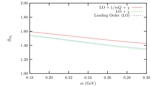
Figure 6: The bag parameter $\hat{B}$ for $B_{d}$

The values for the $f_{B}$’s and especially for the ratio $f_{B_{s}}/f_{B_{d}}$ (and $\xi$) in (75) are a bit low latt ; Ljublj . There might be at least three reasons for this. First, concerning the absolute value for $f_{B}$’s, they dependent significantly on the value of the quark condensate, as seen from equation (45) and (48). In ahjoe we used the “standard” value ${\langle}\,\overline{q}q\,{\rangle}=(-240\,\text{MeV})^{3}$, without any uncertainty. It could be argued that we should have used an uncertainty of 10 MeV, say, for ${\langle}\,\overline{q}q\,{\rangle}^{1/3}$, although the wide range 190 to 250 MeV used for $m$ will to some extent compensate for this. Second, it might be that our expansion within the HL$\chi$QM overestimates the counter-term $\omega_{1}$ which reduces $f_{B_{s}}$. However, neglecting this counter-term would give the high value $f_{B_{s}}/f_{B_{d}}\simeq 1.3$. Third, our value for the axial pion coupling ${g_{{\cal A}}}$ in (28) might be too low. In ahjoe we used input from QCD sum rules beyalev both in the $B$- and $D$-sectors. Alternatively, we may use the experimental value for the effective coupling ${g_{{\cal A}}}^{H^{*}H\pi}=0.59\pm 0.09$ in the $D$-sector anas , giving almost the same bare coupling ${g_{{\cal A}}}=0.59\pm 0.04$. Using this bare coupling also in the $B$-sector (instead of ${g_{{\cal A}}}=0.42\pm 0.06$ in ahjoe ), and in addition ${\langle}\,\overline{q}q\,{\rangle}^{1/3}=(-240\pm 10)\,\text{MeV}$, we obtain an alternative set of values:

$$\tau_{b}=(0.25\pm 0.04)\,\text{GeV}\qquad \delta_{G}=(0.5\pm 0.2)$$ (76)

$$\tau_{\chi_{d}}=-(0.06\pm 0.01)\,\text{GeV}^{2}\qquad \tau_{\chi_{s}}=-(0.25\pm 0.04)\,\text{GeV}^{2}$$

$$\tau^{G}_{\chi_{d}}=-(0.07\pm 0.01)\,\text{GeV}^{2}\qquad \tau^{G}_{\chi_{s}}=(0.2\pm 0.2)\,\text{GeV}^{2}$$

$$\hat{B}_{B_{d}}=1.51\pm 0.09\qquad \hat{B}_{B_{s}}=1.37\pm 0.14$$

$$f_{B_{d}}=(190\pm 50)\,\text{MeV}\qquad f_{B_{s}}=(210\pm 70)\,\text{MeV}$$

$$f_{B}\sqrt{\hat{B}_{B_{d}}}=(240\pm 70)\,\text{MeV}\qquad f_{B_{s}}\sqrt{\hat{B}_{B_{s}}}=(260\pm 90)\,\text{MeV}$$

$$\xi=\frac{f_{B_{s}}\sqrt{\hat{B}_{B_{s}}}}{f_{B_{d}}\sqrt{\hat{B}_{B_{d}}}}=1.08\pm 0.07\qquad \frac{f_{B_{s}}}{f_{B_{d}}}=1.14\pm 0.07$$

We observe that the value for $f_{B_{s}}/f_{B_{d}}$ in (76) is close to the standard one.

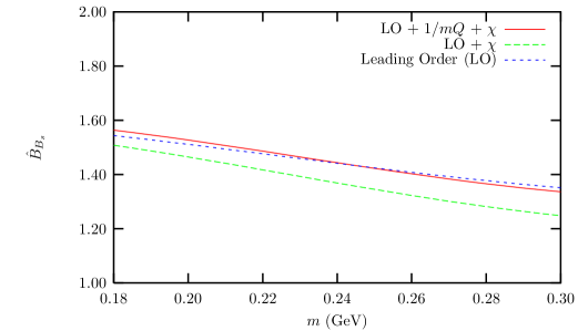
Figure 7: The bag parameter $\hat{B}$ for $B_{s}$

To conclude, we have calculated the bag parameter $\hat{B}$ for the $B_{d}$ and $B_{s}$ mesons. Combining our two alternative sets of values (and consider the range of values) we find $\hat{B}_{B_{d}}=1.51\pm 0.09$ and $\hat{B}_{B_{s}}=1.40\pm 0.16$. The value for $\hat{B}_{B_{s}}$ is more sensitive to chiral loops and counter-terms, and therefore the uncertainty is bigger.

In principle, $\hat{B}$ is renormalization invariant ($\mu$ independent). This cannot be shown within our approach. By construction, perturbative QCD within HQEFT, the HL$\chi$QM and chiral perturbation theory are matched at the scale $\Lambda_{\chi}$. However, we have a reasonable good matching numerically as in BEF . Varying the renormalization scale $\mu=\Lambda_{\chi}$ in the range 0.8 GeV to 1 GeV, the bag parameters only change with 6$\%$. Moreover, like in BEFL , the formula (58) nicely shows the the various parts building up the total result for $\hat{B}$.

Appendix A Loop integrals

The divergent integrals entering in the bosonization of the HL$\chi$QM are defined :

$$I_{1}\, {\,\equiv\,} \,\int\frac{d^{d}k}{(2\pi)^{d}}\frac{1}{k^{2}-m^{2}}$$ (77)

$$I_{3/2}\, {\,\equiv\,} \,\int\frac{d^{d}k}{(2\pi)^{d}}\frac{1}{(v\cdot k)(k^{2}-m^{2})}$$ (78)

$$I_{2}\, {\,\equiv\,}\, \int\frac{d^{d}k}{(2\pi)^{d}}\frac{1}{(k^{2}-m^{2})^{2}}$$ (79)

The integrals needed in the calculation of chiral corrections to the bag parameter are :

$$L^{m,\Delta}_{1,1} =\int\,\frac{d^{d}k}{(2\pi)^{d}}\frac{1}{(k^{2}-m^{2})(v\cdot k-\Delta)}=\frac{-i\Delta}{8\pi^{2}}\left(\frac{1}{{\bar{\varepsilon}}}-\ln(m^{2})+2-2F(m/\Delta)\right)$$ (80)

$$\int\,\frac{d^{d}k}{(2\pi)^{d}}\frac{k^{\mu}k^{\nu}}{(k^{2}-m^{2})(v\cdot k-\Delta)}=A\,g^{\mu\nu}+B\,v^{\mu}v^{\nu}$$

$$A=\frac{1}{d-1}\int\,\frac{d^{d}k}{(2\pi)^{d}}\frac{k^{2}-(v\cdot k)^{2}}{(k^{2}-m^{2})(v\cdot k-\Delta)}$$

$$=\frac{i\Delta}{16\pi^{2}}\left\{(-\frac{1}{{\bar{\varepsilon}}}+\ln(m^{2})-1)(m^{2}-\frac{2}{3}\Delta)-\frac{4}{3}F(m/\Delta)(\Delta^{2}-m^{2})-\frac{4}{3}(m^{2}-\frac{5}{6}\Delta^{2})\right\}$$ (81)

$$B=-A+\int\,\frac{d^{d}k}{(2\pi)^{d}}\frac{(v\cdot k)^{2}}{(k^{2}-m^{2})(v\cdot k-\Delta)}$$

$$=\frac{-i\Delta}{16\pi^{2}}\left\{(-\frac{1}{{\bar{\varepsilon}}}+\ln(m^{2})-1)(2m^{2}-\frac{8}{3}\Delta)-\frac{4}{3}F(m/\Delta)(4\Delta^{2}-m^{2})\right.$$

$$\left.\qquad\qquad-\frac{4}{3}(m^{2}-\frac{7}{3}\Delta^{2})\right\}$$ (82)

where:

$$F(x)=\begin{cases}&-\sqrt{x^{2}-1}\tan^{-1}(\sqrt{x^{2}-1})\qquad x>1\\ &\,\sqrt{1-x^{2}}\tanh^{-1}(\sqrt{1-x^{2}})\qquad x<1\end{cases}$$ (83)

In the case of $\Delta>m$ we have ignored an analytic real part in (80). Equation (80) coincides with the one obtained in GriBo however equation (82) differs by a factor $-2/3(m^{2}-2/3\Delta^{2})$ inside the parenthesis of the expressions for $A$ and $B$. This is presumably due to the factor $1/(d-1)=(1-2/3{\varepsilon})/3$ in $A$.

Appendix B Some detailed expressions for hadronic parameters

The parameters of equation (65) are :

$$\alpha_{3}^{\gamma} {\,\equiv\,}\frac{m}{3}\alpha_{H}+\frac{G_{H}}{6}{\langle}\,\overline{q}q\,{\rangle}$$ (84)

$$\alpha_{3}^{v} {\,\equiv\,}\frac{m}{3}\alpha_{H}+\frac{2}{3}G_{H}{\langle}\,\overline{q}q\,{\rangle}$$

$$\beta_{1} {\,\equiv\,}\frac{G_{B}^{2}\pi^{2}}{12}{\langle}\frac{\alpha_{s}}{\pi}G^{2}{\rangle}$$

$$\beta_{2} {\,\equiv\,}-\frac{f^{2}}{4m^{2}N_{c}}$$

$$\beta_{3} {\,\equiv\,}-\frac{\delta{g_{{\cal A}}}}{4G_{B}^{2}N_{c}}$$

$$\beta_{4} {\,\equiv\,}\frac{1}{8\pi}$$

The $\beta_{K,M}^{(1,2)}$’s in (69) are given by :

$$\beta_{K}^{(1)} = \frac{m}{256\pi^{2}}G_{B}^{2}\left\{1+\frac{4}{\pi}-\frac{8\pi}{N_{c}}\left(\frac{f}{m}\right)^{2}(1+\frac{1}{\rho}-\pi)-\frac{32\pi^{2}}{N_{c}^{2}}\left(\frac{f}{m}\right)^{4}\right.$$ (85)

$$\left.\qquad\qquad\quad-C_{K}\left[\frac{8\pi}{N_{c}}\left(\frac{f}{m}\right)^{2}+\frac{16\pi^{2}}{N_{c}^{2}}\left(\frac{f}{m}\right)^{4}\right]\;\right\}$$

$$\beta_{M}^{(1)} = -\frac{\pi^{2}}{12N_{c}^{2}}\left(\frac{f}{m}\right)^{2}$$ (86)

$$\beta_{M}^{(2)} = \frac{\pi}{24N_{c}}\left\{1+\frac{2\pi}{N_{c}}\left(\frac{f}{m}\right)^{2}\right\}$$ (87)