Nonequilibrium Goldstone phenomenon in Hybrid Inflation

Abstract

We study the onset of Goldstone phenomenon in a hybrid inflation scenario. The physically motivated range of parameters is analyzed in order to meet the cosmological constraints. Classical equations of motion are solved and the evolution through the spontaneous symmetry breaking is followed. We emphasize the role of topological defects that partially maintain the disordered phase well after the waterfall. We study the emergence of the Goldstone excitations and their role in the onset of the radiation dominated universe.

1 Introduction

The real time dynamics of phase transitions is one of the most important topics of nonequilibrium field theory[1] with applications ranging from the description of relativistic heavy ion collisions to cosmological scenarios such as hybrid inflation[2]. The reheating of the universe in this framework has been addressed by several authors[3, 4, 5]. A particularly efficient mechanism, called spinodal (tachyonic) instability sets a sudden end for the inflation by the so called waterfall mechanism. This framework involves a nonthermal phase transition for the matter field that is coupled to the hypothetical inflaton field. The formation and decay of topological or domain structures may play a crucial role in the further evolution of the fields[4, 6].

In this study we concentrate on the Goldstone phenomenon as it emerges in a hybrid inflation scenario. We consider the coupled system of the (scalar) inflaton field ($\sigma$) and a two-component matter field ($\Phi$) in a self-consistently expanding flat and homogeneous FRW metrics with the following Lagrangian:

$${L}=\frac{1}{2}(\partial_{\nu}\sigma(x))^{2}-\frac{1}{2}m_{\sigma}^{2}\sigma^{2}+\frac{1}{2}|\partial_{\nu}\Phi(x)|^{2}-\frac{1}{2}m_{\Phi}^{2}|\Phi|^{2}-\frac{\lambda}{24}|\Phi|^{4}-\frac{1}{2}g^{2}\sigma^{2}|\Phi|^{2},$$ (1)

We solve the classical equations of motion numerically and investigate the dynamics of the to-be-Goldstone modes. A brief discussion is presented first on the choice of cosmologically viable parameters in Eq. (1) and we recall the most important numerical measurement algorithms. Then the onset of Goldstone phenomenon is addressed with emphasis on the late time behaviour of the equation of state.

2 Parameters

Let us concentrate on a GUT-scale ($\sim 10^{15}$ GeV) scalar field that is reheated by the spinodal instability induced by the much lighter ($\sim 10^{12}$ GeV) inflaton field. A natural choice for the GUT self coupling is $\sim 1$. The coupling to the inflaton field is chosen in the range $0.01<g<0.1$ similarly to Copeland et al[4]. This physically motivated range of parameters have to be confronted to our cosmological expectations.

There are two constraints the solution of the model should respect. First, to ensure a successful inflation the total number of e-foldings of the scale factor $a(t)$ should be $\sim 50\dots 100$. The second constraint stems from the relation of the quantum fluctuations of the inflationary period to the density fluctuations measured by the COBE experiment[7]. This relation is due to the superhorizon evolution of the fluctuations which left the horizon during the inflation and reentered again in the recombination era:

$$5\times 10^{-4}=\Bigl{(}\frac{\delta\rho}{\rho}\Bigr{)}_{COBE}=\Bigl{(}\frac{\delta\rho}{\rho+p}\Bigr{)}_{exit}.$$ (2)

($p$ is the pressure of the system). In the terminal phase of the inflation characterized by the Hubble constant $H$ the quantum fluctuations of the inflaton ($\delta\sigma\sim H/2\pi$) dominate:

$$\frac{\delta\rho_{\sigma}}{\rho_{\sigma}+p_{\sigma}}\sim\frac{\delta\sigma V^{\prime}(\sigma)}{\dot{\sigma}^{2}}=\frac{HV^{\prime}(\sigma)}{2\pi\dot{\sigma}^{2}}.$$

During the roll of the inflaton one can directly measure the size of this combination. The modes reentering at recombination made their exit near the end of inflation, therefore we decided to require the COBE estimate to be fulfilled at $\Delta N=5$ e-foldings before the inflation is terminated.

The early dynamics of the hybrid inflation is determined by the evolution of the homogeneous mode of the inflaton field $\sigma_{0}(t)$ and the FRW scale parameter $a(t)$, since the other modes are unoccupied before the onset of spinodal instability. At zero time the inflaton homogeneous mode is set to $\sigma_{0}(t=0)=M_{\mbox{\footnotesize Planck}}$ and $\dot{\sigma}_{0}(t=0)=0$. Then we numerically solve the Einstein equation and the equation of motion for $\sigma_{0}(t)$ and $a(t)$ (the scale parameter of the universe) without relying on the slow-roll condition. We scan through the physically motivated range of parameters and select those models that meet the cosmological constraints. In Fig. 1 we varied the inflaton-matter coupling $g$ keeping $(\lambda/6)^{3/2}/g=1$ fixed (note that this combination appears in the slow-roll approximation to Eq. (2).

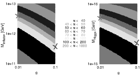
Figure 1: Ranges of parameters that eventuate density fluctuations expected upon the COBE results. The bands refer to different number of e-foldings ($N$). In the present study we concentrate on the set of parameters marked by the dark cross.

In this presentation we discuss numerical results corresponding to the set of parameters marked by the dark cross in Fig. 1. ($g=0.1$, $\lambda=1.29$, $M_{H}=2.2\cdot 10^{15}$ GeV, $m_{\sigma}=3.6\cdot 10^{11}$ GeV.)

3 Measurement techniques for the physical degrees of freedom

In the $O(2)$ hybrid inflation there are three degrees of freedom at each lattice site: the inflaton, and the two components of the $O(2)$ symmetric scalar field. In the broken phase, our intuition is that the independent degrees of freedom are the radial ($\rho(x)=\sqrt{\Phi_{1}^{2}(x)+\Phi_{2}^{2}(x)}$), and the angular ($\rho\phi(x)=\rho\arctan(\Phi_{2}(x)/\Phi_{1}(x)$) fields. (One may think of the radial component as the GUT scale Higgs boson.) In order to test the onset of this idea, we measured the velocity correlation matrix ($W_{ij}$) which is defined by

$$W_{ij}=\frac{\tilde{W}_{ij}}{\sqrt{\tilde{W}_{ii}\tilde{W}_{jj}}},$$

$$\tilde{W}_{ij}=\langle v_{i}v_{j}\rangle-\langle v_{i}\rangle\langle v_{j}\rangle,$$ (3)

where $v_{i}=(\dot{\sigma},\dot{\rho},\rho\dot{\phi})$ stands for velocity-like field components and the brackets mean spatial averaging. The inflaton-Higgs cross correlation can be seen in Fig. 2. It shows a maximum after the tachyonic instability, but it is negligible even then. Its height strongly depends on the parameters but not on the system size. The other two correlators (angular-Higgs and angular-inflaton) are smaller and vanish with increasing volume.

The change of sign of the effective Higgs mass

$$M^{2}_{\mbox{eff}}=m^{2}_{\Phi}+g^{2}\langle\sigma^{2}\rangle+\lambda\langle\rho^{2}\rangle/2$$ (4)

coincides with the exponential growth of the $\langle\rho\rangle$ field (Fig. 2). Later this effective mass relaxes close to the measured gap value of the radial component.

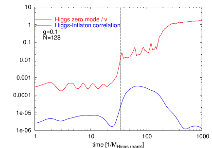
Figure 2: Two stage symmetry breaking: in the first stage, in tachyonic instability, the $O(2)$ field gets excited, only later in the second stage is the symmetry breaking completed. (The vertical lines limit the time interval when the effective mass is negative (see text).) The inflaton-higgs correlation squared ($W_{12}^{2}$) is also displayed.

The masses of the angular and radial field components were extracted from their dispersion relation[8, 9]. The method requires uncorrelated field components in Fourier space $X_{k}$. We measure the quantity ${|\dot{X}_{k}|^{2}}/{|X_{k}|^{2}}$. If only a single frequency ($\omega_{k}$) dominates the motion of a mode, than this ratio is equal to $\omega_{k}^{2}$. Extrapolating this quantity to $k=0$ we get the squared mass gap of the component $X$. In practice we average over different directions in ${\bf k}$ space, over microscopical time scales and over different runs with random initial conditions. We measured the radial (Higgs) mass choosing $X=\rho=\sqrt{\Phi_{1}^{2}+\Phi_{2}^{2}}$, and the angular one with $X=\langle\rho\rangle\exp(i\varphi)$. We fitted the dispersion relation with a polinomial in $k^{2}$. The radial mass was actually extrapolated from the $k>0.75$ region, because of the observed low-$k$ region bending-down (See Fig. 5).

4 Mechanism of Symmetry Breaking

In our simulations we observe a delay in the completion of the symmetry breaking (SB) relative to the tachyonic instability. At the instant of the tachyonic preheating the Higgs expectation value (vev) reaches a finite but very small value. The symmetry is broken in the strict sense but the Higgs vev has not reached the value one would expect from the effective potential yet. At later times the Higgs vev approaches its final value. (In fact, the initial conditions break the O(2) symmetry so that we can observe the SB at the length scale of the lattice size. ($L\approx 90\times M_{H}^{-1}$)).

The sudden growth of the radial component induces large number of domains with different directions of SB. The domain walls are characterized by small values of the radial component. One may also observe extended volumes of small $\rho$, called hot spots[4]. The volume ratio of these hot spots is reflected by the actual value of the $\rho_{0}(t)$ in the period of the incomplete SB.

In momentum space one can easily understand the oscillatory behavior of the OP before the completion of the SB. The inflaton field (still oscillating) has a direct influence on the mass squared of the matter field (see Eq. (4)). The time scale of this oscillation is much slower than the GUT scale so the elementary oscillators of the matter field are tuned adiabatically. The amplitude squared times the frequency is an adiabatic invariant of these oscillators. For $\sigma_{0}(t)\approx 0$ we have a smaller effective mass by Eq. (4) and hence, larger amplitudes and larger value for the OP. Opposingly, for large inflaton values the OP will come closer to zero, this is reflected by a considerably higher volume ratio of hot spots (see Fig. 3). Note that in this regime the value of the effective mass squared is always positive. The growth of the OP during the completion of SB is not of tachyonic nature!

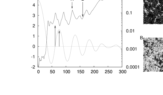
Figure 3: Influence of inflaton zero mode oscillations (dotted, left-hand-side scale) on the OP (solid, right-hand-side scale). At different inflaton values lattice snapshots are displayed. The dark zones refer to large $\rho(x)$ values. We may interpret the light zones as hot spots.

The OP cannot reach its broken phase value as long as the domain structure is present. An easy way to characterize the density of topological defects is to monitor the average of the angular twist $\Sigma_{x}\delta\varphi(x)$ calculated along straight lines. This number is large right after the tachyonic excitations of the matter field, since domains are formed with random orientation. In the completely broken phase it should be zero. The periodic reappearance and dissolution of hot spots erases the domain walls, and eventually the OP departs from the vicinity of zero. As a support of this interpretation we show the coincidence of the vanishing of the twist number and the final growth of the OP in Fig. 4.

Figure 4: The twist number (related to the topological defect density, see text) indicates that the decay of the domain structure coincides with the complete breaking of symmetry. The side plots show the matter field values for the ensemble of lattice sites right before and after the completion of SB.

After the SB is complete, the virial equilibrium of the angular and inflaton modes is soon accomplished ($E_{\mbox{kinetic}}=E_{\mbox{gradient}}+E_{\mbox{potential}}$). Before the onset of virial equlibrium, there is an energy excess in the angular gradient energy, which is due to topological excitations[6].

In the phase of completely broken symmetry the angular matter field components are the Goldstone excitations. In the period of the incomplete SB, however, one should be more careful with the identification. In the following we study how the angular modes start obeying the Goldstone theorem.

We use now the methods reviewed in Sec. 3 to monitor the evolution of the dispersion relation and the onset of the Goldstone theorem.

Figure 5: Dispersion relations for the different matter field components before and after the complete breaking of symmetry. On the early time plot the angular component definitely show a nonvanishing gap, which is absent at late times. This fact encouraged us to refer to the angular modes as “Goldstone” in the second plot.

In Fig. 5 we display the dispersion relation for the radial and angular field components in the partially and completely broken phase. These curves would be straight lines for the physical quasiparticle excitations of the equilibrium theory. The curvature of the dispersion relation mostly indicate the far-from-equilibrium field configuration. The method obviously fails with the radial (Higgs) mode for $k^{2}<0.5$

Fig. 5 (left) clearly demonstrates a nonvanishing gap at early times. This gap, however, is absent in the dispersion relation measured in the broken phase. The gap for both field components may be displayed as a function of time if the measurements are carried out frequently through the evolution. The resulting plot is shown in Fig. 6.

Figure 6: Evolution of the mass gap for the radial (Higgs) and angular field components. The decay of the domain structure coincides with the onset of the Goldstone theorem.

As soon as the OP departs from zero (see Fig. 3) the mass of the angular mode vanishes and stays further in the vicinity of zero. In the presence of domains the mass scale is set by the domain size[9]. To have a gapless excitation this size should grow beyond the lattice size.

5 Equation of state

Equilibrium fields of definite mass obey well defined equations of state (EOS): ultrarelativistic particles obey $\rho=3p$, while for the nonrelativistic matter $p=0$. (Here $\rho$ stands for the energy density, $p$ for the pressure.) The appeareance of well-defined EOS gives a hint how the system arrives to the state of the Hot Universe from the inflaton.

In a nonequilibrium evolution the EOS varies strongly with time. In Fig. 7 (left) we displayed the effective EOS for the full system, which is wildly oscillating. These oscillations are completely averaged out by the solution of the Einstein equations.

Figure 7: Effective equations of state for the full system and the different field compontents (see text).

The early evolution of the energy density is dominated by the inflaton zero mode. If one is interested in the bulk thermodynamics of the microscopic degrees of freedom, this oscillating contribution has to be removed. The contribution of the inflaton zero mode has to be substracted with great care since the potential energy for the matter field is mostly determined by the inflaton zero mode. By making use of the separation of time scales the oscillating part of the inflaton energy is considered to be a contribution of the zero mode, the rest is regarded as the energy contribution of the microscopic degrees of freedom. The equation of state for the disordered motion of the system is also shown in Fig. 7 (left). In Fig. 7 (right) we show the EOS for the different microscopic field components. The curves give the $p-\rho$ paths the field components move along, they are displayed starting shortly before the completion of the SB.

A massive field is expected to fulfil $\rho>3p$, i.e. the corresponding curve should be below the marked straight line in Fig. 7 (right). The curve for the angular component lies slightly above this line. Note that extrapolating the dispersion relation from the high-$k$ modes one would get a negative squared effective mass (see Fig. 5). It is not the gap itself but the entire dispersion relation that determines the EOS the system follows.

Remarkably, the effective EOS for the light fields rapidly converge to the expected straight line behaviour even though the spectral equilibrium is far from being reached. To that time the virial equilibrium is estabilished, although the mode temperatures are different. In fact, in a weakly coupled massless theory each of the elementary oscillators provide the same contribution to $\rho/p$ even if they would assume different mode temperature[6]. In conclusion we can say that the Goldstone excitations begin to play their cosmological role right after the complete SB by yielding a dominant contribution to the pressure and therefore leading the universe into the radiation dominated epoch.

References

- [1] D. Bodeker, Nucl. Phys. Proc. Suppl. 94 (2001) 61
- [2] A. D. Linde, “Lectures on inflationary cosmology,” arXiv:hep-th/9410082; A. D. Linde, Phys. Rev. D 49 (1994) 748
- [3] J. Garcia-Bellido and A. D. Linde, Phys. Rev. D 57 (1998) 6075
- [4] E. J. Copeland, S. Pascoli and A. Rajantie, Phys. Rev. D 65 (2002) 103517
- [5] J. Skullerud, J. Smit and A. Tranberg, W particle distribution in electroweak tachyonic pre-heating, (contribution to this Workshop), arXiv:hep-ph/0210349.
- [6] M. Yamaguchi, Phys. Rev. D 60 (1999) 103511
- [7] E. W. Kolb and M. S. Turner, “The Early Universe,” Addison-Wesley Publishing Company, 1990
- [8] Sz. Borsányi, A. Patkós, D. Sexty Phys. Rev. D 66 (2002) 025014
- [9] Sz. Borsányi, A. Patkós, D. Sexty and Zs. Szép, Phys. Rev. D 64 (2001) 125011
- [10] G. N. Felder, J. Garcia-Bellido, P. B. Greene, L. Kofman, A. D. Linde and I. Tkachev, Phys. Rev. Lett. 87 (2001) 011601