Comment on and Erratum to
β€œPressure of Hot QCD at Large $N_{f}$”

Andreas Ipp
Institut fΓΌr Theoretische Physik, Technische UniversitΓ€t Wien,
Wiedner Hauptstr. 8–10, A-1040 Vienna, Austria
   Guy D. Moore
Department of Physics, McGill University,
3600 rue University, MontrΓ©al, QC H3A 2T8, Canada
   Anton Rebhan
Institut fΓΌr Theoretische Physik, Technische UniversitΓ€t Wien,
Wiedner Hauptstr. 8–10, A-1040 Vienna, Austria
Abstract:

We repeat and correct the recent calculation of the thermodynamic potential of hot QCD in the limit of large number $N_{f}$ of fermions. The new result for the thermal pressure turns out to agree significantly better with results obtained from perturbation theory at small coupling. For large coupling, a nonmonotonic behaviour is reproduced, but the pressure of the strongly coupled theory does not exceed the free pressure as long as the Landau pole ambiguity remains negligible numerically.

1/N Expansion, Thermal Field Theory, QCD
††preprint: TUW-02-26

1 Introduction

In a recent paper [1] the thermal pressure in QCD with a large number of fermions $N_{f}\gg N_{c}\sim 1$ was calculated at next-to-leading order (NLO) in a large $N_{f}$ expansion. Although the large-$N_{f}$ limit is afflicted by the presence of a Landau pole, thermal effects can be studied in a cutoff theory provided the temperature is much smaller than the cutoff which in turn has to be smaller than the scale of the Landau pole. Then at NLO order of the large $N_{f}$ expansion exact results, nonperturbative in the effective coupling $g^{2}_{\rm eff}=g^{2}N_{f}/2$, can be obtained as long as $g^{2}_{\rm eff}\ll 6\pi^{2}$.

Exact large-$N$ results in scalar field theory at finite temperature have been obtained previously and used to study the (poor) convergence properties of thermal perturbation theory [2, 3]. An exact nonperturbative result for a more QCD-like theory is of particular interest in view of the various recent attempts to improve thermal perturbation theory in hot QCD by selective resummations [4, 5, 6, 7, 8], for which it may serve as a testing ground. In Ref.Β [1], it was proposed to interpret a failure of some technique at large $N_{f}$ and reasonably large $g^{2}_{\rm eff}$ as meaning that the technique is certainly not valid in full, small-$N_{f}$ QCD. However, Peshier [9] recently argued that the strong-coupling behaviour of large $N_{f}$ QCD is probably too different from that of small-$N_{f}$ QCD to draw such conclusions.

The result presented in Ref.Β [1] is in fact very different from an ideal quasiparticle picture as pursued in Refs. [10, 11, 12].111A discussion of the HTL-quasiparticle picture of QCD thermodynamics underlying the approach of Ref.Β [6] in the context of large-$N_{f}$ is contained in Ref.Β [13]. According to Ref.Β [1], the gluonic contribution decreases as a function of $g^{2}_{\rm eff}$ only up to a certain value of $g^{2}_{\rm eff}$, after which it rises and even exceeds the free pressure long before the coupling is so strong that the presence of a Landau pole becomes relevant.

In the following, we shall present the numerical result that two of us (A.I.Β and A.R.) have obtained by a new implementation which closely follows the approach of Ref.Β [1]. This result differs from that published by one of us (G.D.M.) in Ref.Β [1], but after correcting the error in the computer code222In evaluating Eq.Β (3.11) of Ref.Β [1], the imaginary part of the logarithm of the longitudinal propagator was calculated as the arctangent of the imaginary part over the real part without checking whether the argument was within the principal branch of the arctangent function. underlying the latter, the two independent evaluations agree to an accuracy better than $1:10^{4}$.

The new result turns out to follow rather closely the perturbative results to order $g^{5}$ up to $g^{2}_{\rm eff}\approx 6$. At $g^{2}_{\rm eff}\approx 12$ the pressure goes through a minimum after which it rises, in qualitative accordance with the result presented in Ref.Β [1], but the exact result starts to exceed the free-gluon pressure only at values of $g^{2}_{\rm eff}>28$, which is so large that the Landau pole starts to influence the results noticeably.
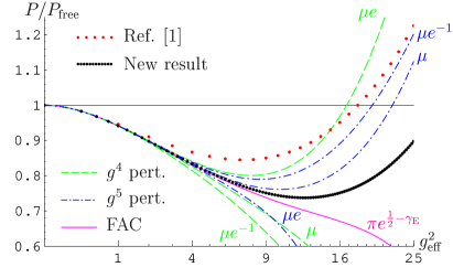
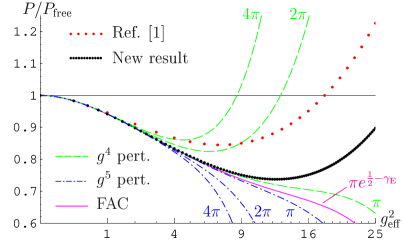
Refer to caption

(a)

Refer to caption

(b)

Figure 1: Exact result for $P_{NLO}/P_{\rm free}$ as a function of $g^{2}_{\rm eff}(\bar{\mu}=\pi e^{-\gamma_{E}}T)$, rendered with an abscissa linear in $g_{\rm eff}$, in comparison with the previous result of Ref.Β [1] and two sets of perturbative results through order $g^{4}$ and $g^{5}$: (a) with renormalization point chosen within a power of $e$ of $\pi e^{-\gamma_{E}}T$; (b) within a power of 2 of $2\pi T$. The line marked β€œFAC” corresponds $\bar{\mu}=\pi e^{{1\over 2}-\gamma_{E}}T$ where the perturbative result to order $g^{4}$ coincides with the one to order $g^{5}$.

2 Results

The NLO contribution to the thermal pressure, of order $N_{f}^{0}$, is given by the one-loop gauge-boson contribution with any number of (renormalized) fermion bubble insertions [1]. Carrying out the sums over Matsubara frequencies, this expression involves terms proportional to the Bose distribution $n_{b}$, which are best calculated in Minkowski space, and parts without this factor, which Ref.Β [1] evaluated partly in Minkowski and partly in Euclidean space. To avoid spurious logarithmic divergences, it is crucial to employ a Euclidean invariant cutoff $\Lambda$ when cutting out the Landau pole. This introduces an error which is suppressed, relative to the full thermal contribution, by $\sim T^{4}/\Lambda^{4}$, so that the ambiguity caused by the Landau singularity is well under control for $\Lambda\gg T$. If the coupling $g^{2}_{\rm eff}\ll 6\pi^{2}$, the Landau pole is exponentially large and one may choose a large cutoff $\Lambda^{2}=a\Lambda^{2}_{\rm Landau}$, which following [1] we shall vary by taking $a$ between $1/4$ and $1/2$.

To ensure Euclidean O(4) invariance when performing parts of the calculation in Minkowski and parts in Euclidean space, which have to be connected by great arcs, one needs the analytic continuation of the complete fermion one-loop self-energy to the complex energy plane. The relevant formulae are listed in the Appendix.

Ref.Β [1] calculated pieces linear in $n_{b}$ in Minkowski space. Terms without $n_{b}$ were computed along a complex frequency contour which ran up the Minkowski axis to $\omega_{\rm max}<\Lambda_{\rm Landau}\sqrt{a}$ for some $a<1$, then along the great arc to Euclidean space, and back down to $q_{0}=\sqrt{q^{2}_{max}-q^{2}}$; finally, a Euclidean integration of the $n_{b}$ free term was performed over 4-spheres in Euclidean space up to $Q^{2}<\Lambda^{2}_{\rm Landau}a$.

It is in fact simpler to calculate all pieces linear in $n_{b}$ in Minkowski space, and all terms without $n_{b}$ in Euclidean space. By actually calculating both ways, we have a rather non-trivial numerical check on the result. In our numerical implementation both ways turned out to agree within numerical errors of about $10^{-5}$.

In Fig.Β 1 we give our numerical result as a function of $g^{2}_{\rm eff}(\bar{\mu}=\pi e^{-\gamma_{E}}T)$.333Tabulated results can be obtained on-line from http://hep.itp.tuwien.ac.at/~ipp/data/ . The new result agrees well with the perturbative results to order $g^{5}$ up to $g^{2}_{\rm eff}\approx 5$, where the renormalization scheme dependence444In contrast to the exact result, the perturbative results depend on the value of the renormalization point $\bar{\mu}$, which we vary between $\pi T$ and $4\pi T$, expressing everything as a function of $g^{2}_{\rm eff}(\bar{\mu}=\pi e^{-\gamma_{E}}T)$, however, to make a comparison possible. of the $g^{5}$-result is still reasonably small (the previous result of Ref.Β [1] showed significant deviations from the perturbative results already for $g^{2}_{\rm eff}\gtrapprox 2$). If the perturbative result to order $g^{5}$ is optimized by fastest apparent convergence (FAC), which requires that the result to order $g^{4}$ coincides with the one to order $g^{5}$ and which amounts to $\bar{\mu}=\pi e^{{1\over 2}-\gamma_{E}}T$, the agreement with perturbation theory is improved and extends to $g^{2}_{\rm eff}\approx 7$.

For higher values of $g^{2}_{\rm eff}$ the exact result flattens out and reaches a minimum at $g^{2}_{\rm eff}\approx 12$. For still higher values the pressure rises but, contrary to the previous result of [1], it does not exceed the free pressure for the range of coupling considered in [1].
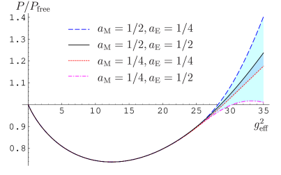
In Fig.Β 2 we consider even higher values of $g_{\rm eff}^{2}$ and find that eventually the thermal pressure grows larger than the free pressure. This occurs at $g_{\rm eff}^{2}>28$ where $\Lambda_{\rm Landau}/T<34$. While this still seems to be a reasonably large number, the numerical result starts to become sensitive to the cutoff just where the pressure approaches the free one. The four curves displayed in Fig.Β 2 show the result of varying the parameter $a$ in the UV cutoff $\sqrt{a}\Lambda_{\rm Landau}$ in the Minkowski and Euclidean parts of the calculation ($a_{M}$ and $a_{E}$, resp.) from $a=1/4$ to $a=1/2$. The numerical result is rather insensitive to this below $g^{2}_{\rm eff}\approx 25$, but very sensitive in the region where the pressure starts to exceed the free one.

Refer to caption
Figure 2: The result for $P_{NLO}/P_{\rm free}$ up to $g_{\rm eff}^{2}=35$ and with different cutoffs.

3 Conclusion

The exact result for the pressure of hot QCD in the limit of large $N_{f}$ shows a nonmonotonic behaviour as a function of the coupling. The minimum of the pressure is reached when $\Lambda_{\rm Landau}\simeq 480T$ and where the ambiguity introduced by the Landau singularity is completely negligible. For higher values of the coupling the pressure eventually reaches and exceeds that of the free theory, but at that point the Landau pole is at $\Lambda_{\rm Landau}<34T$. Above this point the result becomes increasingly sensitive to the precise cutoff which has to be chosen between $T$ and $\Lambda_{\rm Landau}$. This suggests that only the nonmonotonic behaviour is to be taken seriously, but not the fact that the free theory value is eventually reached and exceeded.

So in contrast to the previous result of [1], the corrected one does not imply that an ideal quasiparticle picture (where the pressure has to be smaller than the free one) is necessarily in conflict with the actual physics of QCD in the limit of large fermion number. In order to be compatible with the nonmonotonic behaviour at large coupling, however, a quasiparticle picture would require a correspondingly nonmonotonic behaviour of the quasiparticle masses. While this is not particularly natural for the simple quasiparticle picture underlying the approaches of [10, 11, 12], this is not a priori excluded for the more complicated HTL-based ones of Ref.Β [6]. This issue is discussed in more detail in Ref.Β [13].

Appendix A Appendix: Gauge-boson self-energy

A.1 Spectral representation

A convenient starting point for performing the analytic continuation of the self-energy from Minkowski to Euclidean space or vice versa is its spectral representation

Πμ​ν​(z,𝐩)=βˆ«βˆ’βˆžβˆžd​p02​π​πμ​ν​(p0,p)zβˆ’p0subscriptΞ πœ‡πœˆπ‘§π©superscriptsubscript𝑑subscript𝑝02πœ‹subscriptπœ‹πœ‡πœˆsubscript𝑝0𝑝𝑧subscript𝑝0\Pi_{\mu\nu}(z,\mathbf{p})=\int_{-\infty}^{\infty}\frac{dp_{0}}{2\pi}\frac{\pi_{\mu\nu}(p_{0},p)}{z-p_{0}} (1)

which is valid for any complex $z$ [14]. The spectral form $\pi_{\mu\nu}(p_{0},p)$ is a purely real quantity that can be read off from the fermion loop evaluated in the imaginary time formalism according to

Πμ​ν​(i​ωn,𝐩)superscriptΞ πœ‡πœˆπ‘–subscriptπœ”π‘›π©\displaystyle\Pi^{\mu\nu}(i\omega_{n},\mathbf{p}) $\displaystyle=$ $\displaystyle-4g^{2}_{\rm eff}\int\frac{d^{3}k}{(2\pi)^{3}}\int_{-\infty}^{\infty}\frac{dk_{0}}{2\pi}\int_{-\infty}^{\infty}\frac{dq_{0}}{2\pi}$
$\displaystyle\times\rho_{0}(k_{0},\mathbf{k})\rho_{0}(q_{0},\mathbf{q})\frac{n_{f}(k_{0})-n_{f}(q_{0})}{k_{0}-q_{0}-i\omega_{n}}I^{\mu\nu}(k,q)$

with $I^{\mu\nu}=k^{\mu}q^{\nu}+q^{\mu}k^{\nu}-g^{\mu\nu}k^{\alpha}q_{\alpha}+g^{\mu\nu}m^{2}$ and $\mathbf{q}\equiv\mathbf{k}-\mathbf{p}$. The fermionic distribution function is given by $n_{f}(k_{0})=1/(e^{k_{0}/T}+1)$ and the free spectral function by $\rho_{0}(k_{0},\mathbf{k})=2\pi\epsilon(k_{0})\delta(k_{0}^{2}-\mathbf{k}^{2}-m^{2})=\frac{\pi}{\varepsilon_{k}}(\delta(k_{0}-\varepsilon_{k})-\delta(k_{0}+\varepsilon_{k}))$ with $\epsilon(k_{0})=k_{0}/|k_{0}|$ and $\varepsilon_{k}\equiv\sqrt{\mathbf{k}^{2}+m^{2}}$. (In the following we shall however consider only the ultrarelativistic limit $m/T\to 0$.)

We need separately the transverse and longitudinal projection of the self-energy. Following Weldon [15] we define 2​geff2​G≑gμ​ν​Πμ​ν2superscriptsubscript𝑔eff2𝐺superscriptπ‘”πœ‡πœˆsubscriptΞ πœ‡πœˆ2g_{\rm eff}^{2}G\equiv g^{\mu\nu}\Pi_{\mu\nu} and 2​geff2​H≑uμ​uν​Πμ​ν2subscriptsuperscript𝑔2eff𝐻superscriptπ‘’πœ‡superscriptπ‘’πœˆsubscriptΞ πœ‡πœˆ2g^{2}_{\rm eff}H\equiv u^{\mu}u^{\nu}\Pi_{\mu\nu} with the thermal rest frame velocity $u^{\mu}=(1,0,0,0)$.

Treating the various projections of the spectral density separately, we obtain the following useful representations by analytically performing three of the four integrations:

$$\pi_{X}(p_{0},\mathbf{p})=\pi_{X}^{+}(p_{0},p)-\pi_{X}^{+}(-p_{0},p)$$ (3)
$\displaystyle\pi_{X}^{+}(p_{0},p)$ $\displaystyle=$ $\displaystyle\frac{g^{2}N_{f}}{2\pi p}\int_{0}^{\infty}dk\left(n_{f}(k)-\frac{1}{2}\right)\bar{I}_{X}$
$\displaystyle\times\epsilon(k-p_{0})\theta(|k-p|\leq|k-p_{0}|\leq|k+p|)$

where the $\theta$-function stems from the angular integration between $\mathbf{p}$ and $\mathbf{k}$ (its usage here means $\theta(\textrm{true expression})=1$ and $\theta(\textrm{false expression})=0$) and $X$ = $G$ or $H$ as in

$\displaystyle\bar{I}_{G}\,\equiv\,g^{\mu\nu}I_{\mu\nu}(k_{0}=k)$ $\displaystyle=$ $\displaystyle p_{0}^{2}-p^{2}$ (5)
$\displaystyle\bar{I}_{H}\,\equiv\,u^{\mu}u^{\nu}I_{\mu\nu}(k_{0}=k)$ $\displaystyle=$ $\displaystyle\frac{1}{2}(2k+p-p_{0})(2k-p-p_{0}).$ (6)

The spectral density $\pi$ is manifestly real and odd in $k_{0}$, i.e. $\pi(k_{0},\mathbf{k})=-\pi(-k_{0},\mathbf{k}).$

To subtract the vacuum part, one just has to replace $\left(n_{f}(k)-\frac{1}{2}\right)$ by $n_{f}(k)$. We shall do so in the following explicit results, because the vacuum part requires regularization and renormalization, after which the (Euclidean) self energy simply reads

Ξ vac.μ​ν=βˆ’geff212​π2​(ημ​ν​P2βˆ’Pμ​PΞ½)​(ln⁑P2ΞΌΒ―2βˆ’53).superscriptsubscriptΞ vacπœ‡πœˆsubscriptsuperscript𝑔2eff12superscriptπœ‹2superscriptπœ‚πœ‡πœˆsuperscript𝑃2superscriptπ‘ƒπœ‡superscriptπ‘ƒπœˆsuperscript𝑃2superscriptΒ―πœ‡253\Pi_{\rm vac.}^{\mu\nu}=-{g^{2}_{\rm eff}\over 12\pi^{2}}\left(\eta^{\mu\nu}P^{2}-{P^{\mu}P^{\nu}}\right)\left(\ln{P^{2}\over\bar{\mu}^{2}}-{5\over 3}\right). (7)

A.2 Minkowski result

For Minkowski space we use the Feynman prescription555Note that with our expressions one has to turn the Euclidean $p_{0}$ into the lower half of the complex plane $p_{0}\rightarrow-i\omega+\epsilon$ to obtain the retarded self-energy. Ξ ~F​(p0,𝐩)≑Π​(p0+i​p0​Ρ,𝐩)superscript~Ξ Fsubscript𝑝0𝐩Πsubscript𝑝0𝑖subscript𝑝0πœ€π©\widetilde{\Pi}^{\rm F}(p_{0},\mathbf{p})\equiv\Pi(p_{0}+ip_{0}\varepsilon,\mathbf{p}) for which the self-energy can be separated into

Re​Π~F​(p0,𝐩)=βˆ«βˆ’βˆžβˆžd​p0β€²2​π​π​(p0β€²,p)​Pp0βˆ’p0β€²Resuperscript~Ξ Fsubscript𝑝0𝐩superscriptsubscript𝑑subscriptsuperscript𝑝′02πœ‹πœ‹subscriptsuperscript𝑝′0𝑝Psubscript𝑝0subscriptsuperscript𝑝′0\textrm{Re}\widetilde{\Pi}^{\rm F}(p_{0},\mathbf{p})=\int_{-\infty}^{\infty}\frac{dp^{\prime}_{0}}{2\pi}\pi(p^{\prime}_{0},p)\frac{\textrm{P}}{p_{0}-p^{\prime}_{0}} (8)
Im​Π~F​(p0,𝐩)=βˆ’12​ϡ​(p0)​π​(p0,p).Imsuperscript~Ξ Fsubscript𝑝0𝐩12italic-Ο΅subscript𝑝0πœ‹subscript𝑝0𝑝\textrm{Im}\widetilde{\Pi}^{\rm F}(p_{0},\mathbf{p})=-\frac{1}{2}\epsilon(p_{0})\pi(p_{0},p). (9)

with P denoting the principal value as in $\frac{1}{x+i\varepsilon}=\frac{\textrm{P}}{x}-i\pi\delta(x)$.

Inserting (3) in the expressions (8) and (9) we reproduce the real part of the self-energy as given in Weldon’s paper [15]

$$\textrm{Re}\widetilde{\Pi}_{G}(p_{0},\mathbf{p})=\frac{g^{2}N_{f}}{2\pi^{2}}\int_{0}^{\infty}dk\;n_{f}(k)\left[4k+\frac{p_{0}^{2}-p^{2}}{2p}\log\left|\frac{2k+p_{0}+p}{2k+p_{0}-p}\frac{2k-p_{0}+p}{2k-p_{0}-p}\right|\right]$$

and

$\displaystyle\textrm{Re}\widetilde{\Pi}_{H}(p_{0},\mathbf{p})$ $\displaystyle=$ $\displaystyle\frac{g^{2}N_{f}}{2\pi^{2}}\int_{0}^{\infty}dk\;n_{f}(k)\left[2k\left(1-\frac{p_{0}}{p}\log\left|\frac{p_{0}+p}{p_{0}-p}\right|\right)\right.$ (10)
$\displaystyle\quad\;\left.+\frac{(2k+p_{0}+p)(2k+p_{0}-p)}{4p}\log\left|\frac{2k+p_{0}+p}{2k+p_{0}-p}\right|\right.$
$\displaystyle\quad\;\left.-\frac{(2k-p_{0}-p)(2k-p_{0}+p)}{4p}\log\left|\frac{2k-p_{0}-p}{2k-p_{0}+p}\right|\right].$

The imaginary part was not explicitly calculated by Weldon, but we can provide a completely analytical result where no integration is left to be performed. It is given by

$\displaystyle\textrm{Im}\widetilde{\Pi}_{X}(p_{0},\mathbf{p})$ $\displaystyle=$ $\displaystyle-\frac{1}{2}\epsilon(p_{0})\frac{g^{2}N_{f}}{2\pi p}\left[F^{S}_{X}(\frac{\left|p_{0}+p\right|}{2})-F^{S}_{X}(\frac{\left|p_{0}-p\right|}{2})\right.$ (11)
$\displaystyle\qquad\left.+\epsilon(p_{0}+p)F^{A}_{X}(\frac{\left|p_{0}+p\right|}{2})-\epsilon(p_{0}-p)F^{A}_{X}(\frac{\left|p_{0}-p\right|}{2})\right]$

with symmetric and antisymmetric functions $F_{X}^{S}\equiv(F_{X}^{+}+F_{X}^{-})/2$ and $F_{X}^{A}\equiv(F_{X}^{+}-F_{X}^{-})/2$ that are defined as

$$F^{\pm}_{G}(x)\equiv\int_{x}^{\infty}\;n_{f}(k)\bar{I}_{G}(\pm p_{0},p,k)dk=(p_{0}^{2}-p^{2})F_{1}(x)$$ (12)
$$F^{\pm}_{H}(x)\equiv\int_{x}^{\infty}\;n_{f}(k)\bar{I}_{H}(\pm p_{0},p,k)dk=\frac{p_{0}^{2}-p^{2}}{2}F_{1}(x)\mp 2p_{0}F_{2}(x)+2F_{3}(x),$$

where the $F_{i}(x)$ are the following integrals

$\displaystyle F_{1}(x)$ $\displaystyle\equiv$ $\displaystyle\int_{x}^{\infty}\,n_{f}(k)dk=-x+T\log(e^{x/T}+1),$ (13)
$\displaystyle F_{2}(x)$ $\displaystyle\equiv$ $\displaystyle\int_{x}^{\infty}k\,n_{f}(k)dk=\frac{\pi^{2}T^{2}}{6}-\frac{x^{2}}{2}+xT\log(e^{x/T}+1)+T^{2}\textrm{Li}_{2}(-e^{x/T}),$ (14)
$\displaystyle F_{3}(x)$ $\displaystyle\equiv$ $\displaystyle\int_{x}^{\infty}k^{2}\,n_{f}(k)dk=-\frac{x^{3}}{3}+x^{2}T\log(e^{x/T}+1)$ (15)
$\displaystyle\qquad\qquad\qquad\quad\,\,+2xT^{2}\textrm{Li}_{2}(-e^{x/T})-2T^{3}\textrm{Li}_{3}(-e^{x/T}),$

with $\textrm{Li}_{n}(x)$ being the polylogarithm function. Note that $F_{G}^{A}=0$ simplifies our expression for $\textrm{Im}\widetilde{\Pi}_{G}$ considerably.

A.3 Euclidean result

For Euclidean space we set $z=i\omega$ and (using the antisymmetry property of the spectral density) we get

Re​Π~Eucl​(i​ω,𝐩)=βˆ«βˆ’βˆžβˆžd​p02​π​π​(p0,p)β€‹βˆ’p0Ο‰2+p02,Im​Π~Eucl​(i​ω,𝐩)=0.formulae-sequenceResuperscript~Ξ Euclπ‘–πœ”π©superscriptsubscript𝑑subscript𝑝02πœ‹πœ‹subscript𝑝0𝑝subscript𝑝0superscriptπœ”2superscriptsubscript𝑝02Imsuperscript~Ξ Euclπ‘–πœ”π©0\textrm{Re}\widetilde{\Pi}^{\rm Eucl}(i\omega,\mathbf{p})=\int_{-\infty}^{\infty}\frac{dp_{0}}{2\pi}\pi(p_{0},p)\frac{-p_{0}}{\omega^{2}+p_{0}^{2}},\qquad\textrm{Im}\widetilde{\Pi}^{\rm Eucl}(i\omega,\mathbf{p})=0. (16)

We are left with real integrals of the form

$$\int dp_{0}\frac{-2p_{0}}{\omega^{2}+p_{0}^{2}}\bar{I}_{G}(p_{0},p,k)=-p_{0}^{2}+(\omega^{2}+p_{0}^{2})\log(\omega^{2}+p_{0}^{2})$$ (17)

and

$\displaystyle\int dp_{0}\frac{-2p_{0}}{\omega^{2}+p_{0}^{2}}\bar{I}_{H}(p_{0},p,k)$ $\displaystyle=$ $\displaystyle\frac{1}{2}p_{0}(8k-p_{0})-4k\omega\arctan\left(\frac{p_{0}}{\omega}\right)$ (18)
$\displaystyle-\frac{1}{2}(4k^{2}-p^{2}-\omega^{2})\log(\omega^{2}+p_{0}^{2}).$

With the appropriate integration limits we finally obtain the self-energy in Euclidean space as

Re​Π~G​(i​ω,𝐩)Resubscript~Ξ πΊπ‘–πœ”π©\displaystyle\textrm{Re}\widetilde{\Pi}_{G}(i\omega,\mathbf{p}) $\displaystyle=$ $\displaystyle\frac{g^{2}N_{f}}{2\pi^{2}}\int_{0}^{\infty}dk\;n_{f}(k)\left(4k+\frac{\omega^{2}+p^{2}}{2p}\log\frac{\omega^{2}+(2k-p)^{2}}{\omega^{2}+(2k+p)^{2}}\right)$ (19)
Re​Π~H​(i​ω,𝐩)Resubscript~Ξ π»π‘–πœ”π©\displaystyle\textrm{Re}\widetilde{\Pi}_{H}(i\omega,\mathbf{p}) $\displaystyle=$ $\displaystyle\frac{g^{2}N_{f}}{2\pi^{2}}\int_{0}^{\infty}dk\;n_{f}(k)\left[2k+\frac{\omega^{2}+p^{2}-4k^{2}}{4p}\log\frac{\omega^{2}+(2k-p)^{2}}{\omega^{2}+(2k+p)^{2}}\right.$ (20)
$\displaystyle\,\,\left.-\frac{2k\omega}{p}\left(\arctan\frac{2k-p}{\omega}+2\arctan\frac{p}{\omega}-\arctan\frac{2k+p}{\omega}\right)\right].$

This is in principle the result given in the Appendix of [1] where the three terms involving the arc tangents are replaced by a common logarithm according to

$$\arctan\frac{2k-p}{\omega}+2\arctan\frac{p}{\omega}-\arctan\frac{2k+p}{\omega}=-\frac{i}{2}\log\frac{1+\frac{4k^{2}}{(\omega-ip)^{2}}}{1+\frac{4k^{2}}{(\omega+ip)^{2}}}.$$ (21)

However, while taking the principal branch of the arctan functions gives a smooth function over all $k$, on the right-hand side one must not restrict to the principal branch of the logarithm.

For verifying the path independence of the numerical results we also need the self energy for complex energies. These may be obtained either from the analytic continuation of the results (19) and (20) or from the spectral representation according to

Π​(a+i​b,𝐩)=∫d​p02​π​π​(p0,p)​(aβˆ’p0(aβˆ’p0)2+b2βˆ’i​b(aβˆ’p0)2+b2),Ξ π‘Žπ‘–π‘π©π‘‘subscript𝑝02πœ‹πœ‹subscript𝑝0π‘π‘Žsubscript𝑝0superscriptπ‘Žsubscript𝑝02superscript𝑏2𝑖𝑏superscriptπ‘Žsubscript𝑝02superscript𝑏2\Pi(a+ib,\mathbf{p})=\int\frac{dp_{0}}{2\pi}\pi(p_{0},p)\left(\frac{a-p_{0}}{(a-p_{0})^{2}+b^{2}}-i\frac{b}{(a-p_{0})^{2}+b^{2}}\right), (22)

with real and unambiguous integrals (for bβ‰ 0𝑏0b\neq 0).

Acknowledgments.
This work has been supported by the Austrian Science Foundation FWF, project no. 14632-TPH.

References

  • [1] G.Β D. Moore, Pressure of hot QCD at large $N_{f}$, JHEP 0210 (2002) 055 [hep-ph/0209190].
  • [2] I.Β T. Drummond, R.Β R. Horgan, P.Β V. Landshoff, and A.Β Rebhan, Foam diagram summation at finite temperature, Nucl. Phys. B524 (1998) 579 [hep-ph/9708426].
  • [3] D.Β BΓΆdeker, P.Β V. Landshoff, O.Β Nachtmann, and A.Β Rebhan, Renormalisation of the nonperturbative thermal pressure, Nucl. Phys. B539 (1999) 233 [hep-ph/9806514].
  • [4] J.Β O. Andersen, E.Β Braaten, and M.Β Strickland, Hard-thermal-loop resummation of the free energy of a hot gluon plasma, Phys. Rev. Lett. 83 (1999) 2139 [hep-ph/9902327]; Hard-thermal-loop resummation of the thermodynamics of a hot gluon plasma, Phys. Rev. D61 (2000) 014017 [hep-ph/9905337]; Hard-thermal-loop resummation of the free energy of a hot quark-gluon plasma, Phys. Rev. D61 (2000) 074016 [hep-ph/9908323].
  • [5] J.Β O. Andersen, E.Β Braaten, E.Β Petitgirard, and M.Β Strickland, HTL perturbation theory to two loops, Phys. Rev. D66 (2002) 085016 [hep-ph/0205085].
  • [6] J.Β P. Blaizot, E.Β Iancu, and A.Β Rebhan, The entropy of the QCD plasma, Phys. Rev. Lett. 83 (1999) 2906 [hep-ph/9906340]; Self-consistent hard-thermal-loop thermodynamics for the quark-gluon plasma, Phys. Lett. B470 (1999) 181 [hep-ph/9910309]; Approximately self-consistent resummations for the thermodynamics of the quark-gluon plasma: Entropy and density, Phys. Rev. D63 (2001) 065003 [hep-ph/0005003]; Quark number susceptibilities from HTL-resummed thermodynamics, Phys. Lett. B523 (2001) 143 [hep-ph/0110369].
  • [7] A.Β Peshier, HTL resummation of the thermodynamic potential, Phys. Rev. D63 (2001) 105004 [hep-ph/0011250].
  • [8] P.Β Romatschke, Cold deconfined matter EOS through an HTL quasi-particle model, hep-ph/0210331.
  • [9] A.Β Peshier, Comment on ’Pressure of hot QCD at large $N_{f}$’, hep-ph/0211088.
  • [10] A.Β Peshier, B.Β KΓ€mpfer, O.Β P. Pavlenko, and G.Β Soff, A massive quasiparticle model of the SU(3) gluon plasma, Phys. Rev. D54 (1996) 2399.
  • [11] P.Β Levai and U.Β Heinz, Massive gluons and quarks and the equation of state obtained from SU(3) lattice QCD, Phys. Rev. C57 (1998) 1879 [hep-ph/9710463].
  • [12] A.Β Peshier, B.Β KΓ€mpfer, and G.Β Soff, The equation of state of deconfined matter at finite chemical potential in a quasiparticle description, Phys. Rev. C61 (2000) 045203 [hep-ph/9911474].
  • [13] A.Β Rebhan, HTL resummed thermodynamics of hot and dense QCD: An update, hep-ph/0301130.
  • [14] N.Β P. Landsman and C.Β G. van Weert, Real and imaginary time field theory at finite temperature and density, Phys. Rept. 145 (1987) 141.
  • [15] H.Β A. Weldon, Covariant calculations at finite temperature: The relativistic plasma, Phys. Rev. D26 (1982) 1394.