Electroweak Effects in the Double Dalitz Decay $B_{s}\to l^{+}l^{-}l^{\prime+}l^{\prime-}$

Abstract

We investigate the double Dalitz decays $B_{s}\to l^{+}l^{-}l^{\prime+}l^{\prime-}$ on the basis of the effective Hamiltonian for the transition $b\bar{s}\to l^{+}l^{-}$, and universal form factors suggested by QCD. The correlated mass spectrum of the two lepton pairs in the decay $B_{s}\to e^{+}e^{-}\mu^{+}\mu^{-}$ is derived in an efficient way, using a QED result for meson decays mediated by two virtual photons: $B_{s}\to\gamma^{*}\gamma^{*}\to e^{+}e^{-}\mu^{+}\mu^{-}$. A comment is made on the correlation between the planes of the two lepton pairs. The conversion ratios $\rho_{lll^{\prime}l^{\prime}}=\frac{\Gamma(B_{s}\to l^{+}l^{-}l^{\prime+}l^{\prime-})}{\Gamma(B_{s}\to\gamma\gamma)}$ are estimated to be $\rho_{eeee}=3\times 10^{-4},\rho_{ee\mu\mu}=9\times 10^{-5}\text{ and }\rho_{\mu\mu\mu\mu}=3\times 10^{-5}$, and are enhanced relative to pure QED by $10-30\%$.

1 Introduction

In a recent paper [1] we investigated the decay $B_{s}\to l^{+}l^{-}\gamma\,(l=e,\mu)$, using the effective Hamiltonian for the transition $b\bar{s}\to l^{+}l^{-}$, and obtained a prediction for the conversion ratio

$$\rho_{ll}=\frac{\Gamma(B_{s}\to l^{+}l^{-}\gamma)}{\Gamma(B_{s}\to\gamma\gamma)}$$ (1)

in terms of the Wilson coefficients $C_{7},C_{9}$ and $C_{10}$. An essential ingredient of the calculation was the use of a universal form factor characterising the matrix elements $\left<\gamma|\bar{s}i\sigma_{\mu\nu}(1+\gamma_{5})b|\bar{B}_{s}\right>$ and $\left<\gamma|\bar{s}\gamma_{\mu}(1\pm\gamma_{5})b|\bar{B}_{s}\right>$, as suggested by recent work [2] on QCD in the heavy quark limit $(m_{b}\gg\Lambda_{QCD})$. It was found that the ratio $\rho_{ll}$ was significantly higher than one would expect from a QED calculation of Dalitz pair production $B_{s}\to\gamma^{*}\gamma\to l^{+}l^{-}\gamma$, the difference reflecting the presence of the short-distance coefficients $C_{9},C_{10}$, as well as the universal $1/E_{\gamma}$ behaviour of the QCD-motivated form factor. The purpose of the present paper is to apply the same considerations to the “double Dalitz decay” $B_{s}\to l^{+}l^{-}l^{\prime+}l^{\prime-}$, to determine whether there is similar enhancement of the double conversion ratio

$$\rho_{lll^{\prime}l^{\prime}}=\frac{\Gamma(B_{s}\to l^{+}l^{-}l^{\prime+}l^{\prime-})}{\Gamma(B_{s}\to\gamma\gamma)}\,,$$ (2)

compared to what one would obtain from the QED process $B_{s}\to\gamma^{*}\gamma^{*}\to l^{+}l^{-}l^{\prime+}l^{\prime-}$. We examine also the correlation in the invariant mass of the two lepton pairs, and the nature of the angular correlation between the $l^{+}l^{-}$ and $l^{\prime+}l^{\prime-}$ planes, which is a crucial test of the $B_{s}\to\gamma\gamma$ vertex.

2 Matrix Element and Invariant Mass Spectrum

We begin with the effective Hamiltonian for $b\bar{s}\to l^{+}l^{-}$ [3]

$${\cal H}_{\rm eff} = \frac{\alpha G_{F}}{\sqrt{2}\pi}V_{tb}V^{*}_{ts}\biggl{\{}C^{\rm eff}_{9}(\bar{s}\gamma_{\mu}P_{L}b)\bar{l}\gamma_{\mu}l$$

$$+ C_{10}(\bar{s}\gamma_{\mu}P_{L}b)\bar{l}\gamma_{\mu}\gamma_{5}l$$

$$- 2\frac{C_{7}}{q^{2}}\bar{s}i\sigma_{\mu\nu}q^{\nu}(m_{b}P_{R}+m_{s}P_{L})b\bar{l}\gamma_{\mu}l\biggr{\}}$$

where $P_{L,R}=(1\mp\gamma_{5})/2$ and $q$ is the sum of the $l^{+}$ and $l^{-}$ momenta. Ignoring small $q^{2}-$dependent corrections in $C^{\rm eff}_{9}$, the values of the Wilson coefficients are

$$C_{7}=-0.315,C_{9}=4.334,C_{10}=-4.624\,.$$ (4)

Then, as shown in [4], the matrix element for $\bar{B}_{s}\to l^{+}l^{-}\gamma$ has the form

$${\cal M}(\bar{B}_{s}\to l^{+}l^{-}\gamma) = \frac{\alpha G_{F}}{\sqrt{2}\pi}eV_{tb}V^{*}_{ts}\frac{1}{M_{B_{s}}}\cdot$$

$$\cdot\left[\epsilon_{\mu\nu\rho\sigma}\epsilon^{*\nu}q^{\rho}k^{\sigma}(A_{1}\bar{l}\gamma_{\mu}l+A_{2}\bar{l}\gamma_{\mu}\gamma_{5}l)\right.$$

$$+\left.i(\epsilon^{*}(k\cdot q)-(\epsilon^{*}\cdot q)k_{\mu})(B_{1}\bar{l}\gamma_{\mu}l+B_{2}\bar{l}\gamma_{\mu}\gamma_{5}l)\right]$$

where

$$\begin{split}A_{1}&=C_{9}f_{V}+2C_{7}\frac{M^{2}_{B_{s}}}{q^{2}}f_{T}\,,\\ A_{2}&=C_{10}f_{V}\,,\\ B_{1}&=C_{9}f_{A}+2C_{7}\frac{M^{2}_{B_{s}}}{q^{2}}f^{\prime}_{T}\,,\\ B_{2}&=C_{10}f_{A}\,.\end{split}$$ (6)

The form factors $f_{V},f_{A},f_{T},f^{\prime}_{T}$, defined in Ref. [1], will be taken to have the universal form

$$f_{V}=f_{A}=f_{T}=f^{\prime}_{T}=\frac{1}{3}\frac{f_{B_{s}}}{\Lambda_{s}}\frac{1}{x_{\gamma}}+{\cal O}(\frac{\Lambda^{2}_{QCD}}{E^{2}_{\gamma}})\,,$$ (7)

predicted in the heavy quark approximation $(m_{b}\gg\Lambda_{QCD},m_{b}\gg m_{s})$ in QCD [2]. Here, $\bar{\Lambda}_{s}=m_{B_{s}}-m_{b}\approx 0.5{\rm GeV},x_{\gamma}=2E_{\gamma}/M_{B_{s}}=1-q^{2}/M^{2}_{B_{s}}$, and $f_{B_{s}}\approx 200{\rm MeV}$ is the $B_{s}$ decay constant. The essential feature for our purpose will be the universal $1/x_{\gamma}$ behaviour, the absolute normalization dropping out in the calculation of the conversion ratio. (Corrections to universality are discussed in Ref. [5]).

To obtain the matrix element for $B_{s}\to l^{+}l^{-}l^{\prime+}l^{\prime-}$ we treat the second lepton pair $l^{\prime+}l^{\prime-}$ as a Dalitz pair associated with internal conversion of the photon in $B_{s}\to l^{+}l^{-}\gamma$. From this point on, we will specialise to the final state $e^{+}e^{-}\mu^{+}\mu^{-}$, consisting of two different lepton pairs. This avoids the complications due to the exchange diagram that occurs in dealing with two identical pairs. The matrix element then has the structure

$$\begin{split}{\cal M}(\bar{B}_{s}\to e^{+}e^{-}\mu^{+}\mu^{-})&\sim\frac{e}{k^{2}}(a_{+}(q^{2})L_{+}^{\mu}(q_{1},q_{2})+a_{-}(q^{2})L_{-}^{\mu}(q_{1},q_{2}))L^{\nu}_{em}(k_{1},k_{2})\\ &\cdot[\epsilon_{\mu\nu\rho\sigma}q^{\rho}k^{\sigma}+i(g_{\mu\nu}k\cdot q-k_{\mu}q_{\nu})]\end{split}$$ (8)

where $k$ and $q$ are the four-momenta of the two lepton pairs, $k^{2}$ and $q^{2}$ being the corresponding invariant masses. The currents $L_{\pm}$ and $L_{em}$ are given by

$$\begin{split}L_{\pm}^{\mu}(q_{1},q_{2})&=\bar{u}(q_{1})\gamma^{\mu}(1\pm\gamma_{5})v(q_{2})\,,\\ L_{\rm em}^{\mu}(k_{1},k_{2})&=\bar{u}(k_{1})\gamma^{\mu}v(k_{2})\,.\end{split}$$ (9)

where $k_{1}+k_{2}=k,q_{1}+q_{2}=q$. The coefficients $a_{\pm}(q^{2})$ are related to those in Eq. (6) by

$$a_{\pm}(q^{2})=A_{1}(q^{2})\pm A_{2}(q^{2})\,,$$ (10)

where we have used the fact that for universal form factors, $B_{1,2}=A_{1,2}.$

At this stage, it is expedient to compare the matrix element (8) with the matrix element for double Dalitz pair production in QED. We will make use of the recent analysis of Barker et al.[6], who have studied the reaction ${\rm Meson}\to\gamma^{*}\gamma^{*}\to l^{+}l^{-}\l^{\prime+}l^{\prime-}$, using a vertex for ${\rm Meson}\to\gamma\gamma$ that is a general superposition of scalar and pseudoscalar forms, the matrix element being

$$\begin{split}{\cal M}_{\rm Barker}&=const.\cdot\frac{e}{k^{2}}\frac{e}{q^{2}}L^{\mu}_{em}(q_{1},q_{2})L^{\nu}_{em}(k_{1},k_{2})\\ &\cdot\left[\xi_{P}\,\epsilon_{\mu\nu\rho\sigma}q^{\rho}k^{\sigma}+\xi_{S}(g_{\mu\nu}k\cdot q-k_{\mu}q_{\nu})\right]\,.\end{split}$$ (11)

The coefficients $\xi_{P}$ and $\xi_{S}$ are normalized so that $|\xi_{P}|^{2}+|\xi_{S}|^{2}=1$. (In Ref. [6] they are denoted by $\xi_{P}=\cos\zeta,\xi_{S}=\sin\zeta e^{i\delta}$.)

From this matrix element, Barker et al. have derived the correlated invariant mass spectra for the decay into $e^{+}e^{-}\mu^{+}\mu^{-}$ (ignoring form factors at the $M\gamma^{*}\gamma^{*}$ vertex)

$$\begin{split}\left[\frac{1}{\Gamma_{\gamma\gamma}}\left(\frac{d^{2}\Gamma}{dx_{12}dx_{34}}\right)\right]_{Barker}&=\left(\frac{2\alpha^{2}}{9\pi^{2}}\right)\frac{\lambda_{12}\lambda_{34}\lambda}{w^{2}}(3-\lambda^{2}_{12})(3-\lambda^{2}_{34})\\ &\cdot\left[|\xi_{P}|^{2}\lambda^{2}+|\xi_{S}|^{2}(\lambda^{2}+\frac{3w^{2}}{2})\right]\,.\end{split}$$ (12)

The variables entering the above formula are defined as follows:

$$\begin{split}x_{12}&=(q_{1}+q_{2})^{2}/M^{2}=q^{2}/M^{2}\,,\\ x_{34}&=(k_{1}+k_{2})^{2}/M^{2}=k^{2}/M^{2}\,,\\ x_{1}&=x_{2}=\frac{m^{2}_{1}}{M^{2}}\frac{1}{x_{12}}\,,\\ x_{3}&=x_{4}=\frac{m^{2}_{3}}{M^{2}}\frac{1}{x_{34}}\,,\\ z&=1-x_{12}-x_{34}\,,\\ \lambda_{12}&=\sqrt{(1-x_{1}-x_{2})^{2}-4x_{1}x_{2}}\,,\\ \lambda_{34}&=\sqrt{(1-x_{3}-x_{4})^{2}-4x_{3}x_{4}}\,,\\ w^{2}&=4x_{12}x_{34}\,,\\ \lambda&=\sqrt{z^{2}-w^{2}}\,.\end{split}$$ (13)

Here $m_{1}$ and $m_{3}$ denote the masses of the electron and muon, and $M$ the mass of the decaying meson. The phase space in the variables $x_{12}$ and $x_{34}$ is defined by $x^{0}_{34}<x_{34}<(1-\sqrt{x_{12}})^{2},x^{0}_{12}<x_{12}<(1-\sqrt{x_{34}})^{2}$, where $x^{0}_{12}=4m^{2}_{1}/M^{2},x^{0}_{34}=4m^{2}_{3}/M^{2}$.

We can now adapt the QED result (12) to the process $B_{s}\to e^{+}e^{-}\mu^{+}\mu^{-}$, by comparing the matrix element (11) with that in Eq. (8). The essential observation is that in the approximation of neglecting lepton masses, the vector and axial vector parts of the chiral currents $L^{\mu}_{\pm}$ contribute equally and independently to the invariant mass spectrum. In addition, the matrix element for $B_{s}$ decay corresponds to the QED matrix element considered by Barker et al., if we put $\xi_{P}=1/\sqrt{2},\xi_{S}=i/\sqrt{2}$. This allows us to obtain the invariant mass spectrum for the double Dalitz decay $B_{s}\to e^{+}e^{-}\mu^{+}\mu^{-}$ in electroweak theory:

$$\begin{split}\left[\frac{1}{\Gamma_{\gamma\gamma}}\left(\frac{d\Gamma}{dx_{12}dx_{34}}\right)\right]_{EW}&=\left\{\left[(\eta_{9}+\frac{1}{x_{12}})^{2}+\eta^{2}_{10}\right]+\left[(\eta_{9}+\frac{1}{x_{34}})^{2}+\eta^{2}_{10}\right]\right\}\\ &\cdot\frac{x^{2}_{12}x^{2}_{34}}{x^{2}_{12}+x^{2}_{34}}\left|F(x_{12},x_{34})\right|^{2}\cdot\left[\frac{1}{\Gamma_{\gamma\gamma}}\left(\frac{d\Gamma}{dx_{12}dx_{34}}\right)\right]_{QED}\,,\end{split}$$ (14)

where

$$\left[\frac{1}{\Gamma_{\gamma\gamma}}\left(\frac{d\Gamma}{dx_{12}dx_{34}}\right)\right]_{QED}=\frac{\alpha^{2}}{9\pi^{2}}\frac{\lambda_{12}\lambda_{34}\lambda}{w^{2}}(3-\lambda_{12}^{2})(3-\lambda_{34}^{2})(2\lambda^{2}+\frac{3}{2}w^{2})\,.$$ (15)

Here we have used the abbreviation $\eta_{9}=C_{9}/(2C_{7})$ and $\eta_{10}=C_{10}/(2C_{7})$, introduced in Ref. [1]. The electroweak formula (14) reduces to the QED result in the limit $\eta_{9}=\eta_{10}=0,F(x_{12},x_{34})=1$.

The form factor $F(x_{12},x_{34})$ is chosen to have the universal form

$$F(x_{12},x_{34})=\frac{1}{(1-x_{12})}\frac{1}{(1-x_{34})}\,.$$ (16)

(a possible normalization factor drops out in the calculation of the conversion ratio). This is a plausible (but not unique) generalization of the universal QCD form factor $1/(1-x_{12})$ that occurs in the single Dalitz pair process $B_{s}\to e^{+}e^{-}\gamma$.

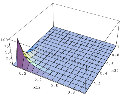
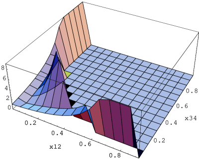
In Fig. 1 we plot the correlated invariant mass spectrum for $B_{s}\to e^{+}e^{-}\mu^{+}\mu^{-}$ in electroweak theory. The ratio of the electroweak and QED spectra is shown in Fig 2, and indicates the effects associated with the coefficients $\eta_{9}$ and $\eta_{10}$, and the form factor $F(x_{12},x_{34})$. One notes a slight depression in the region $x_{12}=-\frac{2C_{7}}{C_{9}}$ or $x_{34}=-\frac{2C_{7}}{C_{9}}$, connected with the vanishing of the term $(C_{9}+\frac{2C_{7}}{x_{12}})^{2}$ or $(C_{9}+\frac{2C_{7}}{x_{34}})^{2}$. 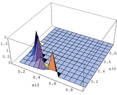There is also a general enhancement for increasing values of $x_{12},x_{34}$, because of the form factor (16). If the form factor $F(x_{12},x_{34})$ is set equal to one, the ratio of the electroweak and QED spectra has the structure plotted in Fig. 3, illustrating the effects which depend specifically on the electroweak parameters $\eta_{9},\eta_{10}$.

The absolute value of the conversion ratio $\rho_{ee\mu\mu}$ is obtained by integrating
$(\frac{1}{\Gamma_{\gamma\gamma}}d\Gamma/dx_{12}dx_{34})_{EW}$ over the range of $x_{12}$ and $x_{34}$. In the QED case, this ratio is conveniently expressed in terms of the integrals $I_{1\ldots 6}$ introduced in Ref. [6]:

$$\begin{split}I_{1}&=\frac{2}{3}\int\int dx_{12}dx_{34}\frac{\lambda^{3}_{12}\lambda^{3}_{34}\lambda^{3}}{w^{2}}\,,\\ I_{2}&=\frac{2}{3}\int\int dx_{12}dx_{34}\frac{\lambda^{3}_{12}\lambda^{3}_{34}\lambda z^{2}}{w^{2}}\,,\\ I_{3}&=\frac{4}{3}\int\int dx_{12}dx_{34}\frac{\lambda^{3}_{12}\lambda^{3}_{34}\lambda^{2}z}{w^{2}}\,,\\ I_{4}&=\int\int dx_{12}dx_{34}\frac{\lambda_{12}\lambda_{34}\lambda^{3}}{w^{2}}(3-\lambda^{2}_{12}-\lambda^{2}_{34})\,,\\ I_{5}&=\int\int dx_{12}dx_{34}\frac{\lambda_{12}\lambda_{34}\lambda z^{2}}{w^{2}}(3-\lambda^{2}_{12}-\lambda^{2}_{34})\,,\\ I_{6}&=\frac{1}{6}\int\int dx_{12}dx_{34}\lambda_{12}\lambda_{34}\lambda(3-\lambda^{2}_{12})(3-\lambda^{2}_{34})\,.\end{split}$$ (17)

These integrals are listed in Table 1 (where, for completeness, we have also given the values for the final states $e\bar{e}e\bar{e}$ and $\mu\bar{\mu}\mu\bar{\mu}$). These integrals allow us to calculate the QED double conversion ratio

$$\begin{split}(\rho_{ee\mu\mu})_{QED}&=\frac{\alpha^{2}}{6\pi^{2}}(I_{1}+I_{2}+2(I_{4}+I_{5}+I_{6}))\\ &=7.6\times 10^{-5}\,.\end{split}$$ (18)

The corresponding result for electroweak theory, based on the differential decay rate (14), can be expressed in terms of the integrals

$$\begin{split}\tilde{I}_{1}&=\frac{2}{3}\int\int dx_{12}dx_{34}\frac{\lambda^{3}_{12}\lambda^{3}_{34}\lambda^{3}}{w^{2}}G(x_{12},x_{34})\,,\\ \tilde{I}_{2}&=\frac{2}{3}\int\int dx_{12}dx_{34}\frac{\lambda^{3}_{12}\lambda^{3}_{34}\lambda z^{2}}{w^{2}}G(x_{12},x_{34})\,,\\ \tilde{I}_{3}&=\frac{4}{3}\int\int dx_{12}dx_{34}\frac{\lambda^{3}_{12}\lambda^{3}_{34}\lambda^{2}z}{w^{2}}G(x_{12},x_{34})\,,\\ \tilde{I}_{4}&=\int\int dx_{12}dx_{34}\frac{\lambda_{12}\lambda_{34}\lambda^{3}}{w^{2}}(3-\lambda^{2}_{12}-\lambda^{2}_{34})G(x_{12},x_{34})\,,\\ \tilde{I}_{5}&=\int\int dx_{12}dx_{34}\frac{\lambda_{12}\lambda_{34}\lambda z^{2}}{w^{2}}(3-\lambda^{2}_{12}-\lambda^{2}_{34})G(x_{12},x_{34})\,,\\ \tilde{I}_{6}&=\frac{1}{6}\int\int dx_{12}dx_{34}\lambda_{12}\lambda_{34}\lambda(3-\lambda^{2}_{12})(3-\lambda^{2}_{34})G(x_{12},x_{34})\,.\end{split}$$ (19)

The factor $G(x_{12},x_{34})$ in the integrand of Eq.(19) contains the effects of the electroweak coefficients $\eta_{9},\eta_{10}$ and the universal form factor $F(x_{12},x_{34})$:

$$\begin{split}G(x_{12},x_{34})&=\left\{\left[\left(\eta_{9}+\frac{1}{x_{12}}\right)^{2}+\eta_{10}^{2}\right]+\left[\left(\eta_{9}+\frac{1}{x_{34}}\right)^{2}+\eta_{10}^{2}\right]\right\}\cdot\\ &\cdot\frac{x^{2}_{12}x^{2}_{34}}{x^{2}_{12}+x^{2}_{34}}\cdot|F(x_{12},x_{34})|^{2}\,.\end{split}$$ (20)

The integrals $\tilde{I}_{1},\ldots,\tilde{I}_{6}$ are given in Table 2. The electroweak conversion ratio, analogous to the QED result (18), is given by

$$\begin{split}(\rho_{ee\mu\mu})_{EW}&=\frac{\alpha^{2}}{6\pi^{2}}\left(\tilde{I}_{1}+\tilde{I}_{2}+2(\tilde{I}_{4}+\tilde{I}_{5}+\tilde{I}_{6})\right)\\ &=9.1\times 10^{-5}\,.\end{split}$$ (21)

In comparison to the QED result (18), the double conversion ratio for $B\to e\bar{e}\mu\bar{\mu}$ in electroweak theory is enhanced by $\sim 20\%$.

A calculation of the spectra for the channels $e\bar{e}e\bar{e}$ and $\mu\bar{\mu}\mu\bar{\mu}$ is complicated by interference between the exchange and direct amplitudes. The conversion ratio for these channels takes the form

$$\rho=\rho_{1}+\rho_{2}+\rho_{12}\,,$$ (22)

where $\rho_{1}$ and $\rho_{2}$ denote the “direct” and “exchange” contribution, and $\rho_{12}$ an interference term. Numerical calculations of the decays $\pi^{0}\to e^{+}e^{-}e^{+}e^{-}$ and $K_{L}\to e^{+}e^{-}e^{+}e^{-}$ suggest that $\rho_{12}$ is small and $\rho_{1}\approx\rho_{2}$. Thus a rough estimate of the double conversion ratio can be obtained using the formula (21), with an extra factor $(\frac{1}{4})\cdot 2$ where $(\frac{1}{4})$ is the statistical factor for two identical fermion pairs, and $2$ comes from adding direct and exchange contributions. This yields, using the numbers in
Table 2

$$\begin{split}(\rho_{e\bar{e}e\bar{e}})_{EW}&\approx 2.9\times 10^{-4}\,,\\ (\rho_{\mu\bar{\mu}\mu\bar{\mu}})_{EW}&\approx 2.8\times 10^{-5}\,.\end{split}$$ (23)

For comparison, the QED results, using Table 1, are

$$\begin{split}(\rho_{e\bar{e}e\bar{e}})_{QED}&\approx 2.7\times 10^{-4}\,,\\ (\rho_{\mu\bar{\mu}\mu\bar{\mu}})_{QED}&\approx 2.2\times 10^{-5}\,.\end{split}$$ (24)

Thus the enhancement in the case of $e\bar{e}e\bar{e}$ is $\sim 10\%$ and that in $\mu\bar{\mu}\mu\bar{\mu}$ about $30\%$. Combining (21) and (23), the ratio of the channels $e\bar{e}e\bar{e},e\bar{e}\mu\bar{\mu}$ and $\mu\bar{\mu}\mu\bar{\mu}$ is approximately

$$\begin{split}e\bar{e}e\bar{e}&:e\bar{e}\mu\bar{\mu}:\mu\bar{\mu}\mu\bar{\mu}\\ =\quad 3&:1:0.3\end{split}$$ (25)

To obtain the absolute branching ratios, we note that the decay rate of $\bar{B}_{s}\to\gamma\gamma$, derived from the effective Hamiltonian (2), involves the Wilson coefficient $C_{7}$ and the universal form factor $f_{T}(x_{\gamma}=1)$ (see Eq. (7)). Using nominal values for $f_{B_{s}}$ and $\bar{\Lambda}_{s}$, and evaluating $C_{7}$ at the renormalization scale $\mu=m_{b}$, Ref. [7] finds ${\rm Br}(B_{s}\to\gamma\gamma)=1.23\times 10^{-6}$. Using this as a reference value, we obtain:

$$\begin{split}{\rm Br}(\bar{B}_{s}\to e\bar{e}e\bar{e})&=3.6\times 10^{-10}\,,\\ {\rm Br}(\bar{B}_{s}\to e\bar{e}\mu\bar{\mu})&=1.1\times 10^{-10}\,,\\ {\rm Br}(\bar{B}_{s}\to\mu\bar{\mu}\mu\bar{\mu})&=3.5\times 10^{-11}\,.\end{split}$$ (26)

3 Correlation of $e^{+}e^{-}$ and $\mu^{+}\mu^{-}$ planes in $\bar{B}_{s}\to e\bar{e}\mu\bar{\mu}$

One of the distinctive features of the electroweak $\bar{B}_{s}\to\gamma\gamma$ matrix element is that the coefficients $\xi_{S}$ and $\xi_{P}$ (normalized to $|\xi_{S}|^{2}+|\xi_{P}|^{2}=1$) are given by $\xi_{S}=\frac{i}{\sqrt{2}}$ and $\xi_{P}=\frac{1}{\sqrt{2}}$. The equality $|\xi_{S}|^{2}=|\xi_{P}|^{2}$ leads to the simplification that the factor $|\xi_{P}|^{2}\lambda^{2}+|\xi_{S}|^{2}(\lambda^{2}+\frac{3}{2}w^{2})$ appearing in the spectrum (12) could be written as $\frac{1}{2}[2\lambda^{2}+\frac{3}{2}w^{2}]$ in going over to the electroweak case (Eq.(15)). A further interesting consequence is the distribution of the angle $\phi$ between the $e^{+}e^{-}$ and $\mu^{+}\mu^{-}$ planes in $\bar{B}_{s}\to e\bar{e}\mu\bar{\mu}$. Generalising the QED result given in Ref. [6] to the electroweak case, the correlation in $\phi$ is given by

$$\left(\frac{1}{\Gamma_{\gamma\gamma}}\frac{d\Gamma}{d\phi}\right)^{e\bar{e}\mu\bar{\mu}}_{EW}=\frac{\alpha^{2}}{6\pi^{3}}\left[\tilde{I}_{1}\sin^{2}\phi+\tilde{I}_{2}\cos^{2}\phi+(\tilde{I}_{4}+\tilde{I}_{5}+\tilde{I}_{6})\right]\,.$$ (27)

The fact that $\tilde{I}_{2}$ is so close to $\tilde{I}_{1}$ means that the spectrum $d\Gamma/d\phi$ is essentially independent of $\phi$. Furthermore, the fact that $arg(\xi_{S}/\xi_{P})=\pi/2$ refelects itself in the absence of a term proportional to $\sin\phi\cos\phi$, the presence of which would lead to an asymmetry between events with $\sin\phi\cos\phi>0$ and $<0$.

It may be remarked that there are corrections to the $B_{s}\to\gamma\gamma$ matrix element (associated, for example, with the elementary process $b\bar{s}\to c\bar{c}\to\gamma\gamma$) which cause the superposition of scalar and pseudoscalar terms to deviate slightly from the ratio $\xi_{S}/\xi_{P}=i$ [7, 8]. From the work of Bosch and Buchalla [7], we find

$$\frac{\xi_{S}}{\xi_{P}}=i\left[1-\frac{2}{3}\frac{C_{1}+NC_{2}}{C_{7}}\frac{\lambda_{B}}{m_{B}}g(z_{c})\right]^{-1}$$ (28)

where

$$g(z)\approx-2+(-2\ln^{2}z+2\pi^{2}-4\pi i\ln z)z+{\cal O}(z^{2})\,,$$ (29)

and $z_{c}=m_{c}^{2}/m^{2}_{b}\sim 0.1,C_{1}=1.1,C_{2}=-0.24,N=3$. There is thus a small correction to the equality $|\xi_{P}|=|\xi_{S}|$. More interestingly, the phase $\delta=arg(\xi_{P}/\xi_{S})$ is not exactly $90^{0}$,implying that a term of the form $\tilde{I}_{3}\sin\phi\cos\phi\cos\delta$ could appear in $d\Gamma/d\phi$. These corrections are, however, too small, to have a measurable impact on the spectrum and branching ratio of the decay $B_{s}\to e\bar{e}\mu\bar{\mu}$ calculated above.

4 Conclusions

We have calculated the spectrum and rate of the double Dalitz decay $\bar{B}_{s}\to e^{+}e^{-}\mu^{+}\mu^{-}$, using the effective Hamiltonian for the flavour-changing neutral current reaction $b\bar{s}\to l^{+}l^{-}$, and form-factors motivated by the heavy quark limit of QCD. A method is given for obtaining the correlated mass spectrum $d\Gamma/dx_{12}dx_{34}$ from the known results for the QED process $\bar{B}_{s}\to\gamma^{*}\gamma^{*}\to e^{+}e^{-}\mu^{+}\mu^{-}$. The conversion ratios $\rho_{l\bar{l}l^{\prime}\bar{l}^{\prime}}=\Gamma(B_{s}\to l^{+}l^{-}l^{\prime+}l^{\prime-})/\Gamma(B_{s}\to\gamma\gamma)$ show an enhancement over the QED result, ranging from $10\%$ for the channel $e^{+}e^{-}e^{+}e^{-}$ to $30\%$ for the channel $\mu^{+}\mu^{-}\mu^{+}\mu^{-}$. Our best estimate of the branching ratios, using the QCD estimate ${\rm Br}(B_{s}\to\gamma\gamma)=1.23\times 10^{-6}$ given in [7], is ${\rm Br}(B_{s}\to e\bar{e}e\bar{e})=3.6\times 10^{-10}$, ${\rm Br}(B_{s}\to e\bar{e}\mu\bar{\mu})=1.1\times 10^{-10},{\rm Br}(B_{s}\to\mu\bar{\mu}\mu\bar{\mu})=3.5\times 10^{-11}$. These branching ratios may have a chance of being observed at future hadron machines producing up to $10^{12}$ $B_{s}$ mesons.

	$B_{s}\to ee\mu\mu$	$B_{s}\to eeee$	$B_{s}\to\mu\mu\mu\mu$
$I_{1}$	7.754	32.501	1.772
$I_{2}$	7.806	32.556	1.821
$I_{3}$	15.556	65.053	3.589
$I_{4}$	17.558	58.416	5.115
$I_{5}$	17.641	58.499	5.199
$I_{6}$	0.0548	0.0556	0.0540

Table 1: Numerical values of the integrals $I_{1},\ldots,I_{6}$ for $B_{s}\to l\bar{l}l^{\prime}\bar{l}^{\prime}$ in QED

	$B_{s}\to ee\mu\mu$	$B_{s}\to eeee$	$B_{s}\to\mu\mu\mu\mu$
$\tilde{I}_{1}$	9.336	35.491	3.856
$\tilde{I}_{2}$	9.477	35.643	4.002
$\tilde{I}_{3}$	18.793	71.114	7.837
$\tilde{I}_{4}$	20.411	63.457	5.784
$\tilde{I}_{5}$	20.637	63.685	6.003
$\tilde{I}_{6}$	0.148	0.152	0.146

Table 2: Numerical values of the integrals $\tilde{I}_{1},\ldots,\tilde{I}_{6}$ for $B_{s}\to l\bar{l}l^{\prime}\bar{l}^{\prime}$ in electroweak theory

Figure 1: Invariant mass distribution $d\Gamma/dx_{12}dx_{34}$ for $B_{s}\to e^{+}e^{-}\mu^{+}\mu^{-}$ in electroweak theory

Figure 2: Ratio $(d\Gamma/dx_{12}dx_{34})_{EW}/(d\Gamma/dx_{12}dx_{34})_{QED}$ showing influence of electroweak parameter $C_{9},C_{10}$ and the form factor $F(x_{12},x_{34})$.

Figure 3: Ratio $(d\Gamma/dx_{12}dx_{34})_{EW}/(d\Gamma/dx_{12}dx_{34})_{QED}$ in the limit of a constant form factor $(F(x_{12},x_{34})=1)$, illustrating specific effect of electroweak parameters $\eta_{9}=C_{9}/(2C_{7})$ and $\eta_{10}=C_{10}/(2C_{7})$.