Statistical Test of Anarchy

Abstract

“Anarchy” is the hypothesis that there is no fundamental distinction among the three flavors of neutrinos. It describes the mixing angles as random variables, drawn from well defined probability distributions dictated by the group Haar measure. We perform a Kolmogorov–Smirnov (KS) statistical test to verify whether anarchy is consistent with all neutrino data, including the new result presented by KamLAND. We find a KS probability for Nature’s choice of mixing angles equal to 64%, quite consistent with the anarchical hypothesis. In turn, assuming that anarchy is indeed correct, we compute lower bounds on $|U_{e3}|^{2}$, the remaining unknown “angle” of the leptonic mixing matrix.

All fermions in the Standard Model of particle physics (SM) seem to come in threes. The three copies of each fundamental matter particle have in common all properties except one – the mass. It is common to say that there are three families, generations, or flavors of each matter particle in the SM. Currently we do not know the reason behind the number three, nor why the matter particles should “repeat” at all. Therefore, it is important to look for any information that may shed light into the origin of flavor.

Within the SM, it has been known for quite some time that different quark flavors can mix quantum mechanically, and that the weak interactions can turn one flavor into another. The “amount” of mixing is summarized by the so-called Cabibbo–Kobayashi–Maskawa (CKM) unitary matrix. The CKM matrix, in turn, can be parameterized by three mixing angles $\theta_{12},\theta_{13},\theta_{23}$ and one complex phase $\delta$ (throughout, we use the “PDG parameterization” PDG for the mixing matrices). A non-vanishing phase $\delta$ indicates that SM processes can violate CP invariance, distinguishing matter from anti-matter in a subtle manner. With the beautiful data from the $B$-factory experiments, we have been able to confirm the CKM framework, and measure all angles and the CP-odd phase with $O(10)\%$ accuracy.

A noteworthy feature of the CKM matrix is that it is rather well approximated by the unit matrix, meaning that the quark mixing angles are all small. This fact, combined with the fact that the quark masses are quite distinct (the ratio of the lightest to heaviest quark mass is $O(10^{-5})$), is interpreted as evidence for the existence of some underlying symmetry or physical mechanism that differentiates the quark families and hence explains the hierarchy in the quark masses and the small mixing angles.

In the SM, all neutrinos are exactly massless. This being the case, one can always choose a basis where the Maki–Nakagawa–Sakata (MNS) unitary matrix, the leptonic analog of the CKM matrix, is the unit matrix without loss of generality. This means that there are no SM processes through which one lepton flavor can turn into another. This hypothesis has been indeed confirmed by all experimental searches for charged lepton flavor violation to date PDG .

If neutrinos have masses, and these masses are distinct, there is no reason to expect that the MNS matrix is trivial, and lepton flavor transitions are observable in principle. In this case, the most sensitive probes for lepton flavor transitions are neutrino oscillation processes, through which a neutrino produced in a well-defined flavor state $\nu_{\alpha}$ is detected in a different flavor state $\nu_{\beta}$ after propagating over a macroscopic distance $L$. The transition probabilities depend on the mixing angles and the CP-odd phase of the MNS matrix, plus the difference of the neutrino masses-squared, $\Delta m^{2}_{ij}\equiv m_{i}^{2}-m_{j}^{2}$.

Since 1998, there is compelling evidence that neutrino flavor transitions do occur when the neutrinos traverse macroscopic distances. Atmospheric atm , solar solar , and, very recently, reactor neutrino experiments KamLAND have all observed data consistent with the neutrino oscillation hypothesis. In light of all the experimental evidence, it appears that neutrinos have masses, and that leptonic flavors mix.

There are two striking features regarding the values of the oscillation parameters which are extracted from the current neutrino data. One is that the neutrino masses are extremely small. Neutrino oscillation experiments have determined that the neutrino mass-squared differences are $|\Delta m^{2}_{23}|=(2-7)\times 10^{-3}$ eV² atm and $\Delta m^{2}_{12}=(4-20)\times 10^{-5}$ eV² KamLAND . These results, combined with direct searches for neutrino masses PDG , yield that the heaviest neutrino mass is less than $O(1)$ eV, over six orders of magnitude smaller than the smallest charged fermion mass of which we know (the electron mass). The other is that, of the mixing angles, two ($\theta_{12},\theta_{23}$) are known with some precision, and are both large: $\sin^{2}2\theta_{23}\gtrsim 0.9$ atm and $\sin^{2}2\theta_{12}\gtrsim 0.4$ KamLAND .

Assuming a three family mixing scenario, there are two more parameters in the MNS mixing matrix that are still unknown: $\theta_{13}$ and $\delta$. In particular, if $\delta\neq 0$ neutrino oscillation processes need not conserve CP. Leptogenesis models leptogenesis , on the other hand, try to relate the existence of matter but no anti-matter in the Universe to the CP violation present in the neutrino sector, making its observation of the utmost interest. CP-violating effects parameterized by the CP-odd phase $\delta$ of the MNS matrix can be probed in accelerator-based long-baseline neutrino oscillation experiments if, for example, one compares the flavor transformation probabilities of neutrinos and anti-neutrinos (written here in vacuum),

$$P(\nu_{e}\rightarrow\nu_{\mu})-P(\bar{\nu}_{e}\rightarrow\bar{\nu}_{\mu})=-16s_{12}c_{12}s_{13}c^{2}_{13}s_{23}c_{23}$$

$$\qquad\sin\delta\sin\frac{\Delta m^{2}_{12}L}{4E}\sin\frac{\Delta m^{2}_{13}L}{4E}\sin\frac{\Delta m^{2}_{23}L}{4E}\ ,$$ (1)

where $s_{ij}=\sin\theta_{ij}$, $c_{ij}=\cos\theta_{ij}$. It is well known that the observation of CP violation in neutrino oscillations is possible only if $\theta_{12}$ and $\Delta m^{2}_{12}$ are “large enough” (and the atmospheric parameters are also large, as has been established by the atmospheric data). The KamLAND result has shown that this is the case. The remaining question, therefore, is whether $\theta_{13}$ is also large enough to render the experimental search for CP violation possible. The only information we currently have is that $\theta_{13}$ is relatively small: $\sin^{2}\theta_{13}\lesssim 0.05$, constrained by the CHOOZ experiment CHOOZ .

The purpose of this letter is two-fold. First, we examine if the current data “requires” new symmetry principles in order to control the structure of the MNS matrix, analogous to the situation in the quark sector. Saying that there is no symmetry principle behind the MNS matrix means there is no fundamental distinction among the three flavors of neutrinos. If this is the case, the MNS matrix is distributed (statistically) according to the bi-invariant Haar measure of group theory, which dictates the probability distribution of the mixing angles. The hypothesis here is that Nature has chosen one point according to this probability distribution. This is the concept of “anarchy” in neutrinos anarchy1 ; anarchy2 . We would like to examine if the data are consistent with anarchy by performing a Kolmogorov–Smirnov (KS) statistical test. We find that they are perfectly consistent.

Second, given the empirical success of anarchy, we study what it has to say about $\theta_{13}$. Anarchy prefers large values for $\theta_{13}$, meaning that a small $\theta_{13}$ would be inconsistent with the anarchical hypothesis. By turning this argument around, we can place a lower limit on $\theta_{13}$ at various confidence levels, again using the KS test.

Consider the following situation: there is a model that “predicts” that a certain quantity is described by a probability distribution. For example, one may construct a model that predicts that a given quantity $x$ may have any value from 0 to 1, with equal probability. This means that the probability density $f(x)$ is

$$f(x)=\left\{\begin{array}[]{ll}1&{\rm if}~{}x\in[0,1],\\ 0&{\rm otherwise.}\end{array}\right.$$ (2)

Let us assume that the value of $x$ is known: $x=x_{0}$. The question to be addressed is how well does the result $x=x_{0}$ agree with the model presented above (that the probability density for $x$ is given by Eq. (2))? This question can be answered using the KS test. Given that we have drawn the specific value $x=x_{0}$, we would like to test the hypothesis ${\cal H}_{f}$ that the probability distribution associated with the random variable $x$ is $f(x)$.

In order to do so we define the distribution function $F(x)\equiv\int_{-\infty}^{x}f(x^{\prime}){\rm d}x^{\prime}$. For Eq. (2),

$$F(x)=\left\{\begin{array}[]{ll}0&{\rm if}~{}x\leq 0,\\ x&{\rm if}~{}x\in[0,1],\\ 1&{\rm if}~{}x\geq 1.\end{array}\right.$$ (3)

We then compare $F(x)$ with the best possible guess for a distribution function $F_{\rm guess}(x)$ that can be obtained given that $x=x_{0}$ has been “drawn,” namely,

$$F_{\rm guess}(x)=\theta(x-x_{0}).$$ (4)

Note that it is very easy to generalize this to $N$ random drawings of $x$, which yield, say, $x_{0},x_{1},\ldots,x_{N-1}$ KS_ref .

The (two-sided) KS statistic (“$D$-function”) is defined by KS_ref

$$D={\rm sup}_{x}[|F_{\rm guess}(x)-F(x)|].$$ (5)

In the example we have been discussing, $D_{0}=x_{0}$ if $x_{0}\geq 0.5$ or $D_{0}=1-x_{0}$ if $x_{0}\leq 0.5$ (note that the two expressions agree at $x_{0}=0.5$, and we assume that $x_{0}\in[0,1]$). If the hypothesis ${\cal H}_{f}$ is correct, the probability that a larger value of $D$ (i.e. a “worse fit”) would be computed from a different random drawing of $x$ is KS_ref

$$P(D\geq D_{0})=2(1-D_{0}),$$ (6)

which is, in the example we have been discussing,

$$P(x_{0})=\left\{\begin{array}[]{ll}2x_{0}&{\rm if}~{}x_{0}\leq 0.5,\\ 2(1-x_{0})&{\rm if}~{}x_{0}\geq 0.5.\end{array}\right.$$ (7)

The smaller the value of $P(x_{0})$, the less likely it is that ${\cal H}_{f}$ is correct. In this context, we allow statements such as ${\cal H}_{f}$ is only allowed at the $[1-P(x_{0})]$ confidence level.

We wish to apply the test described above to the MNS and CKM mixing matrices for leptons and quarks, respectively. Our model is that the mixing matrices are random variables drawn from a “flat” distribution of unitary $3\times 3$ matrices. Following the PDG convention, we define the three mixing angles as in Table 1.

Table 1: $\sin^{2}\theta_{ij}$ in the MNS and CKM mixing matrices, according to the PDG parameterization PDG . In square brackets we quote the currently allowed experimental values for the CKM (MNS) entries at the 90% (three sigma) confidence level.

“angle”	CKM [90% expt.]	MNS [3$\sigma$ expt.]
$\sin^{2}\theta_{13}$	$|V_{ub}|^{2}~{}~{}[(6.2-23)\times 10^{-6}]$	$|U_{e3}|^{2}~{}~{}[0-0.05]$
$\sin^{2}\theta_{12}$	$\sin^{2}\theta_{C}~{}~{}[0.048-0.051]$	$\sin^{2}\theta_{\rm sol}~{}~{}[0.2-0.5]$
$\sin^{2}\theta_{23}$	$|V_{cb}|^{2}~{}~{}[(1.4-1.9)\times 10^{-3}]$	$\sin^{2}\theta_{\rm atm}~{}~{}[0.35-0.65]$

Within this convention, the hypothesis is that the marginalized probability density function is given by (see anarchy2 for a detailed discussion of this point)

$$\int f({U(3)}){\rm d(phases)}=f(\cos^{4}\theta_{13},\sin^{2}\theta_{12},\sin^{2}\theta_{12})=1,$$ (8)

where we have integrated over all (both physical and unphysical) complex phases. The mixing angles are defined such that $\theta_{ij}\in[0,\pi/2],~{}\forall i,j$. The probability distribution is flat in $\sin^{2}\theta_{12}$, $\sin^{2}\theta_{23}$, and $\cos^{4}\theta_{13}$. It is clear that $f=1$ is correctly normalized,

$$\int f~{}{\rm d}(\cos^{4}\theta_{13}){\rm d}(\sin^{2}\theta_{12}){\rm d}(\sin^{2}\theta_{23})=1,$$ (9)

as it should be.

Since anarchy implies that the three mixing angles are distributed as uncorrelated random variables according to Eq. (9), we are allowed to perform a separate KS test for each of the three mixing angles. The three distinct $D$-functions are (from Eq. (5) and the line that succeeds it),

$$D_{\theta^{0}_{13}} = (1-\sin^{2}\theta^{0}_{13})^{2},$$ (10)

$$D_{\theta^{0}_{12}} = 1-\sin^{2}\theta^{0}_{12},$$ (11)

$$D_{\theta^{0}_{23}} = 1-\sin^{2}\theta^{0}_{23}.$$ (12)

The superscript $0$ refers to the randomly picked value (i.e., the physical value, “drawn” by Nature) of the corresponding mixing angle. We have assumed that $\sin^{2}\theta^{0}_{12,23}<1/2$, $\cos^{4}\theta^{0}_{13}>1/2$. The generalization for all values of $\theta_{ij}^{0}$ is trivial and does not add to our discussion .

Because the three “random variables” are not correlated, we calculate the probability that a different random draw would yield a worse result by computing the area where the product of three one-variable probabilities

$$\epsilon^{0} = P(\theta^{0}_{12})\times P(\theta^{0}_{13})\times P(\theta^{0}_{23})$$ (13)

$$= 8\sin^{2}\theta^{0}_{12}(2\sin^{2}\theta^{0}_{13}-\sin^{4}\theta^{0}_{13})\sin^{2}\theta^{0}_{23}$$

is worse than the data. Here, $P(\theta^{0}_{ij})=2(1-D_{\theta^{0}_{ij}})$, as in Eq. (6). Therefore

$$P(KS)=\int{\rm d}(\cos^{4}\theta_{13}){\rm d}(\sin^{2}\theta_{12}){\rm d}(\sin^{2}\theta_{23})\theta(\epsilon-\epsilon^{0}),$$ (14)

where $\epsilon$ is given by the same expression as $\epsilon^{0}$, evaluated at the observed values of the mixing parameters, and $\theta(\epsilon-\epsilon^{0})$ is the usual step function. We obtain

$$P(KS)=\epsilon\left(1-\log\epsilon+\frac{1}{2}\log^{2}\epsilon\right).$$ (15)

By using the best fit values $\sin^{2}\theta_{12}=0.3$ Fogli:2002pb and $\sin^{2}\theta_{23}=0.5$ atm for the MNS matrix, we find

$$\epsilon=2.4(\sin^{2}\theta_{13}-\frac{1}{2}\sin^{4}\theta_{13}).$$ (16)

Given the bound $\sin^{2}\theta_{13}\lesssim 0.05$, the anarchical hypothesis is consistent with the current data, with probability $64\%$.

One can also check whether anarchy works in the quark sector. Using the values tabulated in Table 1, one obtains a probability smaller than $6\times 10^{-6}$, implying that the hypothesis that the CKM matrix is a random unitary $3\times 3$ matrix is safely discarded. Hence, a fundamental distinction among the three flavors of quarks seems to be required.

Once we have established as consistent the hypothesis that the MNS matrix is a matrix drawn from a random sample of unitary $3\times 3$ matrices, we now turn the argument around, and try to place a lower limit on $\theta_{13}$. What we require is that $P(KS)>1-P_{0}$, where $P_{0}$ is defined to be the confidence level of the limit.

Fig. 1 depicts $P(KS)$ for the MNS matrix as a function of $\sin^{2}\theta_{13}\equiv|U_{e3}|^{2}$ within the three sigma bounds allowed experimentally for $\sin^{2}\theta_{12}\equiv\sin^{2}\theta_{\rm sol}$ and $\sin^{2}\theta_{23}\equiv\sin^{2}\theta_{\rm atm}$, as tabulated in Table 1. For the best fit values of $\sin^{2}\theta_{\rm atm}$ and $\sin^{2}\theta_{\rm sol}$, one is able to “rule out” $|U_{e3}|^{2}<0.0007$ at the two sigma level and $|U_{e3}|^{2}<0.00002$ (which is, curiously, the upper bound for $|V_{ub}|^{2}$) at the three sigma level. Fig. 1 also depicts $P(KS)$ as a function of $\sin^{2}\theta_{13}\equiv|V_{ub}|^{2}$ for the CKM matrix within the 90% experimentally allowed ranges defined in Table 1.

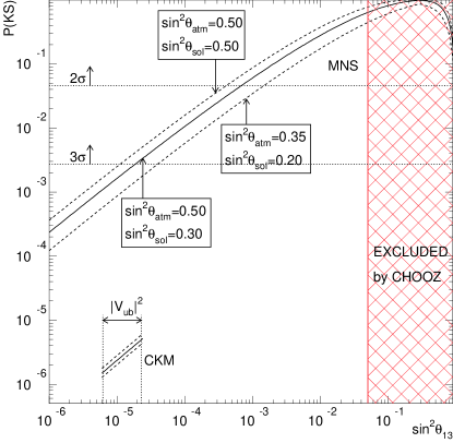
Figure 1: $P(KS)$ for the MNS matrix as a function of $\sin^{2}\theta_{13}\equiv|U_{e3}|^{2}$, see text for details. The top dashed curve corresponds to $\sin^{2}\theta_{\rm sol}=\sin^{2}\theta_{\rm atm}=0.5$, while the bottom dashed curve corresponds to $\sin^{2}\theta_{\rm sol}=0.2$ and $\sin^{2}\theta_{\rm atm}=0.35$. The solid curve corresponds to the best fit values $\sin^{2}\theta_{\rm sol}=0.3$ and $\sin^{2}\theta_{\rm atm}=0.5$. The hatched region is currently excluded by the neutrino data. In the bottom left corner, $P(KS)$ for the CKM matrix as a function of $\sin^{2}\theta_{13}\equiv|V_{ub}|^{2}$ is also depicted within the experimentally allowed range for $|V_{ub}|^{2}$, assuming that the values of $|V_{cb}|^{2}$ and $\sin^{2}\theta_{C}$ vary within the range indicated in Table 1.

Note, however, that these bounds are obtained a posteriori, and turn out to be rather weak. This is due to the fact that the observed values of the angles $\theta_{12}$ and $\theta_{23}$ agree “too well” with the anarchical hypothesis, hence allowing a larger-than-usual fluctuation for $\theta_{13}$. We believe that $P(KS)$ is a good tool for testing the anarchical hypothesis against the data, but not as useful a tool for studying what values of $|U_{e3}|^{2}$ are preferred by the hypothesis. For this reason, we choose to make use of another method of obtaining lower bounds on $|U_{e3}|^{2}$ assuming anarchy. This method can be thought of as yielding an a priori prediction for $|U_{e3}|^{2}$, which, we believe, is more appropriate, and will be described promptly.

Let us compute the marginalized probability density function of $\theta_{13}$ only. From Eq. (9),

$$\int f~{}{\rm d}(\sin^{2}\theta_{12}){\rm d}(\sin^{2}\theta_{23})\equiv g(\cos^{4}\theta_{13})=1.$$ (17)

This probability distribution ($g$) is rather similar to $f$, (see Eq. (9)) but is to be interpreted in a slightly different way. Remember that $f$ is the probability distribution function derived for $U(3)$ marginalized over all CP-odd phases, including: three unphysical phases that can be removed by redefining fermionic SM fields, two “Majorana phases” which may or may not be physical, depending on whether or not the neutrinos are Majorana fermions, and one “Dirac phase.” Marginalyzing over unphysical phases is the only reasonable procedure to follow, and we have chosen to also marginalize over the physical phase(s) in order to address whether the current information we have on mixing angles fits the anarchical hypothesis. This choice only makes sense if the anarchical hypothesis for the “whole” MNS matrix is consistent, which is the case as we have observed above. Similarly, $g$ is the probability distribution function derived for $U(3)$ marginalized over all CP-odd phases and the “solar” and “atmospheric” mixing angles.

The single variable probability is

$$P(KS)_{1d}=P(\theta_{13}^{0})=4(\sin^{2}\theta_{13}-\frac{1}{2}\sin^{4}\theta_{13}).$$ (18)

Fig. 2 depicts $P(KS)_{1d}$ as a function of $\sin^{2}\theta_{13}\equiv|U_{e3}|^{2}$. Again, we can interpret $P(KS)_{1d}$ as the probability that a “worse fit” is obtained assuming that $\theta_{13}$ is a random variable drawn from the probability distribution Eq. (17). These bounds are a priori predictions of the anarchy unlike the previous ones, and should be taken more seriously. We exclude $|U_{e3}|^{2}<0.011$ (0.0007) at the two (three) sigma confidence level. Note that the CKM-equivalent $P(KS)_{1d}=P(V_{ub})$ is less than $10^{-4}$ (this can be easily read off from Fig. 2), again indicating that the anarchical hypothesis in the quark sector can be safely discarded.

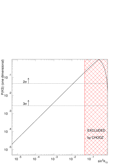
Figure 2: $P(KS)_{1d}$ as a function of $\sin^{2}\theta_{13}\equiv|U_{e3}|^{2}$, see text for details. The hatched region is currently excluded by the neutrino data.

Finally, It is worth recalling that anarchy predicts a flat probability distribution for the CP-violating phase $\delta$ anarchy2 , and hence the distribution in $\sin\delta$ is $1/|\cos\delta|$, peaked at $\sin\delta=\pm 1$. If anarchy is correct, chances are that the observation of CP violation in long-baseline oscillation experiments is indeed within reach!

We now summarize our results, with more discussions to follow. We have statistically tested the hypothesis that the MNS matrix is a matrix drawn from a random “flat” sample of unitary $3\times 3$ matrices. According to the KS test performed, this “anarchical hypothesis” is consistent with the data. The anarchical hypothesis fails the KS test when it is performed with the CKM matrix. Our result is different from other attempts to statistically “test” anarchy. For example, the authors of no_anarchy have claimed that the neutrino sector prefers the existence of some symmetry behind neutrino masses and mixing angles to completely random entries. We have not attempted to perform such a “compartive test,” which is, at least, hard to interpret in a well defined way. We do not believe that such tests are capable of indicating whether one hypothesis is favored with respect to the other. Our test has a well defined statistical interpretation, and directly probes whether anarchy in the neutrino sector is a good hypothesis.

Having checked that anarchy is consistent with our current understanding of the MNS matrix, we were able to use the anarchical hypothesis to “predict” the value of the still unobserved mixing angle $\theta_{13}$. At the two sigma level, anarchy requires that $\sin^{2}\theta_{13}>0.011$, for example (bound obtained from $P(KS)_{1d}$, see Fig. 2). If there is indeed no structure in the leptonic mixing matrix, it seems very likely that one should be able to observe CP-violation in long-baseline neutrino oscillation experiments, as not only are all angles large, but the CP-odd parameter $\sin\delta$ is also “predicted” to be large.

We have nothing to say about the value of the neutrino masses. The hypothesis we tested is that the MNS matrix is “random,” independent of whether the masses are degenerate, partially degenerate or hierarchical anarchy2 . Even in the case of non-LMA solutions to the solar neutrino puzzle (currently ruled out at 99.95% C.L. KamLAND ), one can obtain random mixing matrices min_model . Incidently, it is interesting to note that the the neutrino masses seem to be “less hierarchical” than the charged fermion masses. Assuming that the neutrino masses are not degenerate, it turns out that $m_{3}/m_{2}\simeq\sqrt{\Delta m^{2}_{23}/\Delta m^{2}_{12}}=3-13$, not too far away from unity (of course, we do not know $m_{2}/m_{1}\ldots$). This is consistent with random mass matrices generated via the seesaw mechanism anarchy1 .

We would like to underline important assumptions and limitations of our result. By hypothesis, the probability distributions for the mixing angles are uncorrelated. Our discriminatory procedure does not include information regarding whether the different variables are more likely to be correlated than not. Given the minimal statistics (provided by the fact that we live in only one Universe), adding this sort of information would not lead to different conclusions, although one should start to worry if, say, it turns out that $\sin^{2}2\theta_{23}=\sin^{2}2\theta_{12}=1$. One should also be warned that the KS test performed here need not be the most powerful test for the anarchical hypothesis, statistically speaking KS_ref .

Finally, we emphasize what our result does not imply. Although the anarchical hypothesis is consistent with the data, neutrino mass models which rely on flavor symmetries and nontrivial “textures” are not disfavored in any well defined way. Some are perfectly justified by top-down arguments, including, say, grand unification of matter fields. We would like to point out, however, that the “burden of proof” is with the models that assume that there is structure in the leptonic mixing matrix. The anarchical hypothesis may be viewed as the simplest of flavor models – a model of flavor without flavor. In light of our long experience with quark masses and mixing angles, it is remarkable that, in the neutrino sector, one can do without new symmetry principles in order to appreciate the entries of the MNS mixing matrix.

Note Added – After the first version of the this manuscript became publicly available, a preprint discussing our results Espinosa appeared. All of the comments contained there apply to this version of our manuscript as well. While we appreciate most of the arguments contained in Espinosa , we disagree with its author in a few key points. Most importantly, we do not agree with the claim that $\sin^{2}\theta_{12},\sin^{2}\theta_{23},\cos^{4}\theta_{13}\in[0,1]$ are “angular variables.” Note that the Haar measure is flat in these variables rather than in the mixing angles, which are convention dependent. Therefore we stand by our claim that a KS test can be used to test the anarchical hypothesis. Furthermore, Espinosa contains an alternative statistical test of the anarchical hypothesis (a Kuiper’s test, see Espinosa for details), and the result that maximal mixing is “preferred” is obtained, in qualitative agreement with the results presented here. The author of Espinosa , however, dismisses the result of the Kuiper’s test, claiming that the statistical sample is too small. While we appreciate that some are uneasy about the statistics of very small data samples, namely one chosen by Mother Nature, we point out that the dismissal of such results is not mathematically justified.

- (1) Particle Data Group (K. Hagiwara et al.), Phys Rev. D 66, 010001 (2002).
- (2) Y. Fukuda et al. [Super-Kamiokande Collaboration], Phys. Rev. Lett. 81, 1562 (1998).
- (3) Q. R. Ahmad et al. [SNO Collaboration], Phys. Rev. Lett. 89, 011301 (2002); 011302 (2002).
- (4) K. Eguchi et al. [KamLAND Collaboration], hep-ex/0212021.
- (5) M. Fukugita and T. Yanagida, Phys. Lett. B174, 45 (1986).
- (6) M. Apollonio et al. [CHOOZ Collaboration], Phys. Lett. B466, 415 (1999).
- (7) L.J. Hall, H. Murayama, and N. Weiner, Phys. Rev. Lett. 84, 2572 (2000).
- (8) N. Haba and H. Murayama, Phys. Rev. D 63, 053010 (2001).
- (9) See, e.g., V.K. Rohatgi and A.K. Md. Ehsanes Saleh, “An Introduction to Probability and Statistics,” New York, 1976.
- (10) See, e.g., G. L. Fogli, G. Lettera, E. Lisi, A. Marrone, A. Palazzo and A. Rotunno, Phys. Rev. D 66, 093008 (2002) [arXiv:hep-ph/0208026].
- (11) V. Antonelli, F. Caravaglios, R. Ferrari, and M. Picariello, Phys. Lett. B549, 325 (2002); G. Altarelli, F. Feruglio, and I. Masina, JHEP 0301, 035 (2003).
- (12) See, for example, A. de Gouvêa and J.W. Valle, Phys. Lett. B501, 115 (2001).
- (13) J. R. Espinosa, hep-ph/0306019.