Light meson resonances from unitarized Chiral Perturbation Theory

Abstract

We report on our recent progress in the generation of resonant behavior in unitarized meson-meson scattering amplitudes obtained from Chiral Perturbation Theory. These amplitudes provide simultaneously a remarkable description of the resonance region up to 1.2 GeV as well as the low energy region, since they respect the chiral symmetry expansion. By studying the position of the poles in these amplitudes it is possible to determine the mass and width of the associated resonances, as well as to get a hint on possible classification schemes, that could be of interest for the spectroscopy of the scalar sector.

1 The light meson puzzle

In this work we review our recent progress in determining the position of the poles prep that appear associated to resonant behavior in meson-meson scattering amplitudes, obtained from unitarized one-loop Chiral Perturbation Theory GomezNicola:2001as . This apparently formal interest is motivated by the spectroscopy of light mesons, whose present status is somewhat controversial. Poles in the second Riemann sheet of partial wave scattering amplitudes are of relevance because when they are close to the real, physical values of the center of mass energy $\sqrt{s}$, we can neglect all other terms in the partial wave and simply write

$$t(s)=\frac{R_{R}}{s-s_{pole}}=\frac{R_{R}}{s-(\hbox{Re}\sqrt{s_{pole}})^{2}-(\hbox{Im}\sqrt{s_{pole}})^{2}-i\,2\,\hbox{Re}\sqrt{s_{pole}}\;\hbox{Im}\sqrt{s_{pole}}}$$ (1)

where $R_{R}$ would be some real residue that can be calculated but is irrelevant for us here. Furthermore, if by “close to the real axis” we mean that Im$\sqrt{s_{pole}}\ll$Re$\sqrt{s_{pole}}$, then, we can approximate:

$$t(s)\simeq\frac{R_{R}}{s-(\hbox{Re}\sqrt{s_{pole}})^{2}-i\,2\,\hbox{Re}\sqrt{s_{pole}}\;\hbox{Im}\sqrt{s_{pole}}}\equiv\frac{R_{R}}{s-M_{R}^{2}+i\,M_{R}\,\Gamma_{R}}$$ (2)

where in order to write our equation in the familiar Breit-Wigner form, in the last step we have identified $\sqrt{s_{pole}}\simeq M_{R}-i\Gamma_{R}/2$. Breit-Wigner (BW) resonances yield the familiar and experimentally distinct resonant shape in the cross section and its associated fast phase movement, which increases by $\pi$ in a very small energy range. The quantum numbers of the resonances correspond to those of the partial wave where the pole is sitting.

However, the farther away from the real axis the poles are, the lousier becomes the connection with resonance parameters. Let us remark that in order to have a BW shape, it is essential for the pole to be near the real axis, or more quantitatively $M_{R}\gg\Gamma_{R}$. This allows us to neglect all other terms in the amplitude as well as terms of order $\Gamma_{R}^{2}/M_{R}^{2}$. Intuitively, the familiar resonances that are clearly seen or detected are quasi bound states whose decay time is large (their width is small) compared with their rest energy (their mass). Of course, between a nice BW resonant shape and the continuum, one could think of all intermediate situations, which, naively correspond to changing the pole position from the vicinity of the real axis to have an infinite imaginary part. In other words, starting from narrow resonances and moving the pole to $-i\,\infty$, we get broader structures, and finally, the continuum.

In particular, broad resonant structures seem to occur in the scalar channels in meson-meson scattering, where in the last decade there has been a renewed interest newsigma ; Dobado:1992ha on the longstanding controversy about the existence of a broad scalar-isoscalar resonance in the low energy region: the so called $\sigma$, or $f_{0}(600)$ in the latest version of the Particle Data Group (PDG) Review PDG . Its experimental evidence only from $\pi\pi$ scattering is rather confusing, since it definitely does not display a Breit-Wigner shape, although many groups have been able to identify an associated pole in the amplitude, but deep in the complex plane A similar or even more confusing situation occurs in $\pi K$ scattering, where another pole, the $\kappa$, has been suggested by many groups kappa ; Oller:1997ng , but again there is no trace of a BW shape in the scattering. For an compilation of $\sigma$ and $\kappa$ poles see the nice overview in vanBeveren:2002vw .

Let us remark that meson-meson scattering data pipidata are hard to obtain. As a matter of fact the problem is that they have been extracted from reactions like meson-$N\rightarrow$meson-meson-$N$, but with assumptions like a factorization of the four meson amplitude, or that only one meson is exchanged and that it is more or less on shell, etc… All these approximations introduce large systematic errors. There are, however, other sources of information on meson-meson interactions like, for instance, the very precise determination of a combination of $\pi\pi$ phase shifts from $K_{l4}$ decays Pislak:2001bf . At higher energies the decays of even heavier particles can be also used to study the previously mentioned and other scalar resonances like the $f_{0}(980)$ or the $a_{0}(980)$. For instance, very recently, results from charm decays charm , seem to find both the $\sigma$ and $\kappa$ poles in reasonable agreement with the groups mentioned above, but the controversy about their existence still lingers on.

Meson spectroscopy aims at classifying the bound states of QCD and at identifying their nature, that is, what are they made of. Starting with the scalar-isoscalar sector, its relevance is twofold: First, one of the most interesting features of QCD is its non-abelian nature, which implies that the carriers of the strong force, the gluons, interact among themselves, contrary to what happens with photons in QED. A possible consequence of this fact is the existence of bound states of gluons, or glueballs, which will certainly be isoscalars. In particular, the lightest ones are expected to be also scalars. Naively, once all the members of quark multiplets are identified in the scalar-isoscalar sector, what remains, if any, are good candidates for glueballs. Of course, the whole picture is much more messy due to mixing phenomena, so that the resonances we actually see are a superposition of different kind of states. Second, it is also understood that QCD has an spontaneous breaking of the chiral symmetry since its vacuum is not invariant under chiral transformations. The study of the scalar-isoscalar sector is relevant to understand the QCD vacuum, which has precisely those quantum numbers.

Nevertheless, we should not forget the other channels, since we can find there the other members of the multiplets, since all the channels are related by the chiral SU(3) symmetry of QCD. We cannot simply add BW resonances to different channels without carefully taking into account this symmetry. Concerning vector channels, there are clear BW resonances like the $\rho(770)$ in $\pi\pi$ scattering or the $K^{*}(892)$ in $\pi K$ scattering, that the meson spectroscopy community identify with $q\bar{q}$ states. These are so clearly resonant that “vector meson dominance” is basically enough to describe the bulk of meson interactions.

2 Poles from Chiral Symmetry and Unitarity

The interest of our work in the context of meson spectroscopy is that we have been able to generate the resonant behavior present in meson-meson scattering. Our amplitudes GomezNicola:2001as have been obtained by unitarizing the one-loop amplitudes obtained from Chiral Perturbation Theory (ChPT chpt ), which is the most general effective Lagrangian built of pions, kaons and etas, that respects the chiral symmetry constraints of QCD. However, since the ChPT amplitudes behave as polynomials at high energy, they violate partial wave unitarity, which is imposed with unitarization methods: in our case, the Inverse Amplitude Method (IAM) Dobado:1996ps ; Dobado:1992ha . Note that the resonances are not included explicitly.

Part of this program had been first been carried out for partial waves in the elastic region Dobado:1996ps ; Dobado:1992ha , for which a simple single channel approach could be used, finding the $\rho$ and $\sigma$ poles in $\pi\pi$ scattering and that of $K^{*}$ in $\pi K\rightarrow\pi K$. For coupled channel processes, an approximate form of this approach had already been shown Oller:1997ng to yield a remarkable description of the whole meson-meson scattering data up to 1.2 GeV. When these partial waves were continued to the second Riemann sheet, several poles were found, corresponding to the $\rho$, $K^{*}$, $f_{0}$, $a_{0}$, $\sigma$ and $\kappa$ resonances ( note that the $\kappa$ pole could have also been obtained in the elastic single channel formalism ). The approximations were needed because at that time not all the ChPT meson-meson amplitudes were known to one-loop. Hence, in Oller:1997ng only the leading order and the dominant s-channel loops were considered in the calculation, neglecting crossed and tadpole loop diagrams. Of course, in this way the ChPT low energy expansion could only be recovered at leading order. Concerning the divergences, they were regularized with a cutoff, which violates chiral symmetry, making them finite, but not cutoff independent. Fortunately, the cutoff dependence was rather weak and the description of the data was remarkable for cutoffs of the size of the chiral scale. Nevertheless, due to this cutoff regularization, it was not possible to compare the eight parameters of the chiral Lagrangian, which are supposed to encode the underlying QCD dynamics, with those obtained from other low energy processes. That is, it was not possible to test the compatibility of the chiral parameters with the values already present in the literature.

Of course, due to the controversial nature, or even the doubts about the existence of the scalar states, it is very important to check that the poles are not just artifacts of the approximations, to estimate the uncertainties in their parameters, and to check their compatibility with other experimental information regarding ChPT. That was the reason why, in a first step, the $K\bar{K}\rightarrow K\bar{K}$ one-loop amplitudes were calculated in Guerrero:1998ei , also unitarizing them coupled to the $\pi\pi$ states, and reobtaining the $\sigma$, $f_{0}$ and $\rho$ poles. The whole calculation of one-loop meson meson scattering has been recently completed with the totally new $K\eta\rightarrow K\eta,\eta\eta\rightarrow\eta\eta$ and $K\eta\rightarrow K\pi$ amplitudes GomezNicola:2001as . In addition the other five existing independent amplitudes have also been recalculated. The reason for repeating those existing calculations is that, to one loop, one could choose to write all amplitudes in terms of just $f_{\pi}$, or use all $f_{\pi}$, $f_{K}$ and $f_{\eta}$, or any other combination of them that is equivalent up to $O(p^{4})$ etc… However, when one choice is made for one amplitude, the other ones have to be calculated consistently in order to keep the coupled channel perturbative unitarity, which is needed for the IAM. As commented before, with these unitarized amplitudes we obtained GomezNicola:2001as a simultaneous description of meson meson scattering data in the resonant region up to 1.2 GeV, but also of the low energy region, with scattering lengths compatible with the most recent determinations. The fact that the calculation was complete to one loop and renormalized as in standard ChPT, also allowed us to show that the resulting set of chiral parameters was compatible with previous determinations in the literature.

The final step is therefore to extend analytically the amplitudes to the complex plane and search for poles in the second Riemann sheet. We will provide next a brief account of how we have built our amplitudes, how the data have been fitted, but also our first, preliminary, results for the poles, although a more detailed exposition and the final calculations will be presented somewhere else soon prep .

3 Chiral Perturbation Theory amplitudes

The QCD massless Lagrangian for the light $u,d$ and $s$ quarks is invariant under the $SU(3)_{L}\times SU(3)_{R}$ chiral symmetry, which rotates the Left (or Right) components of these quarks among them. There is also an small explicit breaking due to the small masses of those quarks, but at sufficiently high energies that effect should be rather small. Nevertheless the $SU(3)_{L}\times SU(3)_{R}$ symmetry is not seen in the physical spectrum, but only $SU(3)_{L+R}$ is realized approximately once the small explicit breaking is taken into account. The familiar isospin is nothing but the $SU(2)_{L+R}$ subgroup. The $SU(3)_{L-R}$ symmetry has to be spontaneously broken, and indeed, the pions, kaons and etas can be identified as the associated Goldstone bosons of this breaking. Once more, they are not massless, due to the small masses of those quarks, but they are much lighter (and much more stable) than other hadrons with their same quantum numbers, and than the generic hadronic scale of approximately 1 GeV.

These Goldstone bosons are expected to be the relevant degrees of freedom at low energies. Their low energy dynamics can then be described weinberg by the most general Lagrangian made of pions, kaons and etas, that implements the symmetry breaking pattern described above, as well as other usual constraints like Lorentz invariance, locality, etc… This is called Chiral Perturbation Theory chpt , and it corresponds to an expansion in external momenta, the energy or the mass of the mesons, generically $p$, over the chiral scale $\Lambda=4\pi f_{\pi}\simeq 1.2\,$GeV. The leading term, $O(p^{2})$ is nothing but the non-linear sigma model and only depends on the meson masses and the chiral scale $4\pi f$, where $f$ is the meson decay constant at leading order. Since there are no more free parameters, it is universal, i.e., independent of the detailed mechanism of symmetry breaking. It is enough to reproduce the current algebra results of the 60’s. At next to leading order $O(p^{4})$, there are eight terms which now are multiplied by some arbitrary low energy constants $L_{i}(\mu)$, also called chiral parameters. These parameters contain information on the specific dynamics of the underlying theory, but are also needed for the renormalization of the divergences that appear at one-loop when one uses vertices from the lowest order Lagrangian. This renormalization procedure can be carried out to more loops by adding higher order terms in the Lagrangian. In this way it is possible to obtain finite calculations order by order, at the price of including an increasing number of parameters. However, these new terms will all be suppressed by additional powers of $p^{2}/\Lambda^{2}$ so that the lowest orders will be dominant at low energies. For our purposes it will be enough to work at one-loop, that is $O(p^{4})$, so that we still have amplitudes with imaginary parts, as well as the eight $L_{i}$ parameters that contain information on the specific QCD dynamics.

Therefore, the lowest order, ${\cal O}(p^{2})$, meson-meson scattering amplitudes (called “low energy theorems” weinberg because as we have just commented, they only depend on the symmetry breaking scale) are obtained just from the tree level diagrams of the lowest order Lagrangian. In contrast, the calculation of the ${\cal O}(p^{4})$ contribution involves the evaluation of the following Feynman diagrams: First, the tree level graphs with the second order Lagrangian, which depend on the chiral parameters $L_{i}$. Second, the one-loop diagrams in Fig.1, whose divergences will be absorbed in the $L_{i}$ through renormalization.

In particular, those graphs in Fig.1a provide an imaginary part to ensure perturbative unitarity, whereas those graphs in Fig.1e, provide the wave function, mass and decay constant renormalizations. As we will see the renormalization of the decay constant will play a subtle role in the determination of the $f_{0}(980)$ and $a_{0}(980$) pole positions. Let us then explain this somewhat technical point: Note that the meson decay constants $f_{\pi}\simeq 94.4$MeV, $f_{K}=1.22f_{\pi}$ and $f_{\eta}=1.3f_{\pi}$ only differ at $O(p^{4})$ chpt ; GomezNicola:2001as . At leading order, all of them are equal to the only scale in the Lagrangian, $f$, which, after renormalization, is not directly the physical observable. As a consequence, if we want to write our amplitudes in terms of observable quantities, we could substitute $f$ by $f_{\pi}$ or $f_{K}$ or $f_{\eta}$, or any combination of them. We could even make a different choice for each amplitude as long as we do not couple the amplitudes among them. However, if one wants to study a coupled channel process, once a choice is made for one amplitude, the choices for the coupled amplitudes have to be made consistently, if one wants to ensure perturbative unitarity. The same argument would follow for the masses, but they already differ at leading order, so that the numerical difference is irrelevant compared with the decay constant case.

The one-loop amplitudes of $\pi\pi\rightarrow\pi\pi$ chpt , $\pi K\rightarrow\pi K$ Kpi and that of $\pi\eta\rightarrow\pi\eta$ Kpi were calculated more than a decade ago, because the thresholds of these reactions is low enough to apply the standard ChPT formalism. As explained in the introduction, the $K\bar{K}\rightarrow K\bar{K}$ one-loop amplitudes were calculated in Guerrero:1998ei , and those of $K\eta\rightarrow K\eta,\eta\eta\rightarrow\eta\eta$ and $K\eta\rightarrow K\pi$ in GomezNicola:2001as , much more recently since their thresholds are much higher and they only became interesting when the appropriate unitarization methods were developed. In GomezNicola:2001as , the other five one-loop amplitudes were recalculated in order to express all of them in terms of $f_{\pi}$ only, and ensure exact perturbative partial wave unitarity, which we explain in the next section.

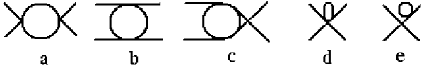
Figure 1: Generic one-loop Feynman diagrams that have to be evaluated in meson-meson scattering.

As we have already commented in the introduction, meson-meson scattering data is customarily presented using partial waves of definite isospin and angular momentum, $t_{IJ}$. In particular the data is given in terms of the complex phase of the amplitude, or phase shifts $\delta_{IJ}$ According to our previous discussion, the meson-meson partial waves within ChPT are thus obtained as series in the momenta, ( some terms are also multiplied by chiral logarithms from the loops functions). Generically, in the chiral expansion we will then find, omitting the $I,J$ subindices, $t\simeq t_{2}+t_{4}+...$, where $t_{2}$ and $t_{4}$ the ${\cal O}(p^{2})$ and ${\cal O}(p^{4})$ contributions, respectively.

4 Partial wave unitarity

The $S$ matrix unitarity relation $SS^{\dagger}=1$ translates into simple relations for the elements of the $T$ matrix $t^{\alpha\beta}$ if they are projected into partial waves, where $\alpha,\beta,...$ denote the different states physically available. For instance, if there is only one possible state, $\alpha$, the partial wave $t^{\alpha\alpha}$ satisfies

$${\mbox{Im}\,}t^{\alpha\alpha}=\sigma_{\alpha}\,|\,t^{\alpha\alpha}|^{2}\quad\Rightarrow\quad{\mbox{Im}\,}\frac{1}{t^{\alpha\alpha}}=-\sigma_{\alpha}\quad\Rightarrow\quad t^{\alpha\alpha}=\frac{1}{{\mbox{Re}\,}t^{\alpha\alpha}-i\,\sigma_{\alpha}}$$ (3)

where $\sigma_{\alpha}=2q_{\alpha}/\sqrt{s}$ and $q_{\alpha}$ is the C.M. momentum of the state $\alpha$. Written in this way it can be readily noted that we only need to know the real part of the Inverse Amplitude. The imaginary part is fixed by unitarity. As a matter of fact, this relation only holds above threshold up to the energy where another state, $\beta$, is physically accessible. Above that point, the unitarity relation for the partial waves can be written as:

$${\mbox{Im}\,}t^{\alpha\alpha} = \sigma_{\alpha}\,|\,t^{\alpha\alpha}|^{2}+\sigma_{\beta}\,|\,t^{\alpha\beta}|^{2},$$ (4)

$${\mbox{Im}\,}t^{\alpha\beta} = \sigma_{\alpha}\,t^{\alpha\alpha}\,t^{\beta\alpha\;*}+\sigma_{\beta}\,t^{\alpha\beta}\,t^{\beta\beta\;*},$$

$${\mbox{Im}\,}t^{\beta\beta} = \sigma_{\alpha}\,|\,t^{\alpha\beta}|^{2}+\sigma_{\beta}\,|\,t^{\beta\beta}|^{2}.$$

or, in matrix form (and only above the second threshold):

$${\mbox{Im}\,}T=T\,\Sigma\,T^{*}\quad\Rightarrow\quad{\mbox{Im}\,}T^{-1}=-\Sigma\quad\Rightarrow\quad T=({\mbox{Re}\,}T-i\,\Sigma)^{-1}$$ (5)

with

$$T=\left(\begin{array}[]{cc}t^{\alpha\alpha}&t^{\alpha\beta}\\ t^{\alpha\beta}&t^{\beta\beta}\\ \end{array}\right)\quad,\quad\Sigma=\left(\begin{array}[]{cc}\sigma_{\alpha}&0\\ 0&\sigma_{\beta}\\ \end{array}\right)\,,$$ (6)

which allows for a straightforward generalization to the case of $n$ accessible states. Once more, unitarity means that we would only need to calculate the real part of the inverse amplitude matrix.

Coming back to ChPT, we can notice that the perturbative series of ChPT behave as polynomials with a higher order term $O(p^{N}/\Lambda^{N})$. If we substitute them in the above unitarity relations for the imaginary parts of $T$, which are non-linear, we will have $O(p^{N}/\Lambda^{N})$ on the left side, but $O(p^{2N}/\Lambda^{2N})$ on the right. Hence, ChPT amplitudes will never satisfy unitarity exactly. Nevertheless, ChPT partial waves satisfy unitarity perturbatively, that is, instead of eq.(3), they can satisfy:

$${\mbox{Im}\,}t_{2}^{\alpha\alpha}=0,\quad{\mbox{Im}\,}t_{4}^{\alpha\alpha}=\sigma_{\alpha}\,|\,t_{2}^{\alpha\alpha}|^{2}$$ (7)

for the single channel case, and instead of eq.(5), they can satisfy

$${\mbox{Im}\,}T_{2}=0,\quad{\mbox{Im}\,}T_{4}=T_{2}\,\Sigma\,T_{2}^{*}$$ (8)

for the coupled channel case. Note that , as we did for a single channel, we are using $T_{2}$ and $T_{4}$ for the $O(p^{2})$ and $O(p^{4})$ contributions to the scattering matrix. We say “can satisfy” because, generically, the above expressions for the one-loop contributions do not hold exactly, but only up to $O(p^{6})$. However, when expressed in terms of physical decay constants, the above relations can even be satisfied exactly if the substitution of $1/f$ in terms of $1/f_{\pi}$ or $1/f_{K}$ or $1/f_{\eta}$ is made to match their corresponding powers on both sides of the above equations. In such case, the $O(p^{6})$ can be made to vanish. (As we already commented, the masses also suffer the same subtlety and the same care has to be taken with them.)

Since in the literature the amplitudes had been calculated sometimes just in terms of $1/f_{\pi}$ but some other times using or $1/f_{K}$ or $1/f_{\eta}$ independently, we recalculated all of them in terms of just $f_{\pi}$ in GomezNicola:2001as , the simplest choice. Nevertheless, we are also presenting here results with the much more natural choice of using the decay constants associated to each field in the process. From the formal point of view, the two choices are equivalent up to $O(p^{4})$, but in the second one the resummation of the decay constants is implicitly carried out to higher orders. In addition, it has the advantage of using $f_{K}$ when dealing with kaons or $f_{\eta}$ when dealing with etas. Numerically, the differences could be sizable at high energies when using the unitarized amplitudes.

5 Unitarization: The Inverse Amplitude Method

Unitarity is a very important feature of scattering, and it is even more relevant when dealing with resonances, which generically saturate the unitarity bounds. This can be illustrated in the single channel case, where eq.(3) implies the following unitarity bound: $|t_{\alpha\alpha}|\leq 1/\sigma_{\alpha}$. Moreover, if we sit on top of a BW resonance, at $s=M_{R}^{2}$, we see from eq.(2), that the amplitude becomes purely imaginary, that is Im$\,t_{\alpha\alpha}=|t_{\alpha\alpha}|$, and therefore, in this case eq.(3) implies $|t_{\alpha\alpha}|=1/\sigma_{\alpha}$. The unitarity bound is saturated. Once more, the ChPT amplitudes if extrapolated to high enough energies, will violate also this bound, since they behave as polynomials in $s$.

In order to unitarize the ChPT amplitudes one of the simplest methods is to introduce the ${\mbox{Re}\,}T$ in eq.(5), calculated as a ChPT expansion

$$T^{-1} \simeq T_{2}^{-1}(1-T_{4}T_{2}^{-1}+...),$$ (9)

$${\mbox{Re}\,}T^{-1} \simeq T_{2}^{-1}(1-({\mbox{Re}\,}T_{4})T_{2}^{-1}+...).$$ (10)

Taking into account the perturbative unitarity conditions, eq.(8), we thus find

$$T^{IAM}\simeq T_{2}(T_{2}-T_{4})^{-1}T_{2},$$ (11)

which is the coupled channel Inverse Amplitude Method, which we have indeed used to unitarize simultaneously the whole set of one-loop ChPT meson-meson scattering amplitudes. Let us remark that if we reexpand eq.(11) at low energies, we recover the vary same chiral expansion, $T^{IAM}=T_{2}+T_{4}+...$, which ensures that we are respecting the QCD chiral symmetry breaking pattern at low energies. In addition, it can be easily checked that $T^{IAM}$ satisfies the partial wave unitarity conditions, eq.(5), exactly, above the thresholds of all the physically accessible channels. Let us also mention that the IAM can be also generalized to higher orders Dobado:1996ps ; Nieves:2001de , including the case when the leading order $t_{2}$ vanishes Dobado:2001rv .

Let us finally remark that the IAM violates crossing symmetry, since obviously we are treating the right and the left cuts differently. The largest influence of the worse left cut approximation is on the closest point to the left cut, that is, the thresholds. We will see that the IAM threshold parameters are in good agreement both with data and with standard ChPT (which certainly respects crossing symmetry), therefore the crossing symmetry violation coming from the IAM itself seems to be small. However, as we have already explained, the meson-meson data is obtained using strong extrapolations. Hence, even the data carries its own amount of crossing violation if errors are not taken into account. When considering not only threshold data, but also experimental information in other regions, including their uncertainties it can be shown that the IAM yields indeed just an small crossing symmetry violation Nieves:2001de .

6 THE INVERSE AMPLITUDE METHOD FIT TO THE SCATTERING DATA

Once we had all the amplitudes calculated within the standard ChPT renormalization scheme (dimensional regularization in the $\overline{MS}-1$ scheme), we first looked at the results using the IAM with previous determinations of the chiral parameters from other processes (see the ChPT column in Table 1). Due to their large error bars, the uncertainties thus obtained were rather large, but all the resonant behavior in meson-meson scattering was clearly recovered. For the detailed plots, we refer the reader to GomezNicola:2001as , but this already suggests that a description of the resonances is possible within the uncertainty limits of the chiral parameters.

Parameter	$K_{l4}$ decays	ChPT	IAM I	IAM II	IAM III
$L_{1}^{r}(M_{\rho})$	$0.46$	$0.4\pm 0.3$	$0.56\pm 0.10$	$0.59\pm 0.08$	$0.60\pm 0.09$
$L_{2}^{r}(M_{\rho})$	$1.49$	$1.35\pm 0.3$	$1.21\pm 0.10$	$1.18\pm 0.10$	$1.22\pm 0.08$
$L_{3}$	$-3.18$	$-3.5\pm 1.1$	$-2.79\pm 0.14$	$-2.93\pm 0.10$	$-3.02\pm 0.06$
$L_{4}^{r}(M_{\rho})$	0 (fixed)	$-0.3\pm 0.5$	$-0.36\pm 0.17$	$0.2\pm 0.004$	0 (fixed)
$L_{5}^{r}(M_{\rho})$	$1.46$	$1.4\pm 0.5$	$1.4\pm 0.5$	$1.8\pm 0.08$	$1.9\pm 0.03$
$L_{6}^{r}(M_{\rho})$	0 (fixed)	$-0.2\pm 0.3$	$0.07\pm 0.08$	$0\pm 0.5$	$-0.07\pm 0.20$
$L_{7}$	$-0.49$	$-0.4\pm 0.2$	$-0.44\pm 0.15$	$-0.12\pm 0.16$	$-0.25\pm 0.18$
$L_{8}^{r}(M_{\rho})$	$1.00$	$0.9\pm 0.3$	$0.78\pm 0.18$	$0.78\pm 0.7$	$0.84\pm 0.23$

Table 1: Different sets of chiral parameters ($\times 10^{3}$). The first column comes from recent analysis of $K_{l4}$ decays BijnensKl4 ($L_{4}$ and $L_{6}$ are set to zero). In the ChPT column $L_{1},L_{2},L_{3}$ come from BijnensGasser and the rest from weinberg . The three last ones correspond to the values from the IAM including the uncertainty due to different systematic error used on different fits. Sets II and II are obtained using amplitudes expressed in terms of $f_{\pi}$, $f_{K}$ and $f_{\eta}$, whereas the amplitudes in set I are expressed in terms of $f_{\pi}$ only.

Of course, a much better description could be obtained with a fit to the data. We therefore carried out a fit, using MINUIT MINUIT , to the presently available data on meson-meson scattering. Due to the already commented problems with the systematic uncertainties in the data, which has not been quantified in the original articles, we performed fits adding a $1\%$, $3\%$ or a $5\%$ systematic error. The resulting curves are basically indistinguishable to the naked eye. The errors quoted in Table 1 for the IAM sets of fitted chiral parameters, correspond to those of MINUIT combined with a systematic error that covers the spread of values obtained when adding that $1\%$, $3\%$ or $5\%$ systematic error. Note that the values we obtain are compatible with previous determinations. In particular, we show in Table 2 the threshold parameters compared with existing data and plain ChPT determinations to one and two loops.

Threshold	Experiment	IAM fit I	ChPT ${\cal O}(p^{4})$	ChPT ${\cal O}(p^{6})$
parameter		GomezNicola:2001as	Dobado:1992ha ; Kpi	Amoros:2000mc
$a_{0\,0}$	0.26 $\pm$0.05	0.231${}^{+0.003}_{-0.006}$	0.20	0.219$\pm$0.005
$b_{0\,0}$	0.25 $\pm$0.03	0.30$\pm$ 0.01	0.26	0.279$\pm$0.011
$a_{2\,0}$	-0.028$\pm$0.012	-0.0411${}^{+0.0009}_{-0.001}$	-0.042	-0.042$\pm$0.01
$b_{2\,0}$	-0.082$\pm$0.008	-0.074$\pm$0.001	-0.070	-0.0756$\pm$0.0021
$a_{1\,1}$	0.038$\pm$0.002	0.0377$\pm$0.0007	0.037	0.0378$\pm$0.0021
$a_{1/2\,0}$	0.13…0.24	0.11${}^{+0.06}_{-0.09}$	0.17
$a_{3/2\,0}$	-0.13…-0.05	-0.049${}^{+0.002}_{-0.003}$	-0.5
$a_{1/2\,1}$	0.017…0.018	0.016$\pm$0.002	0.014
$a_{1\,0}$		0.15${}^{+0.07}_{-0.11}$	0.0072

Table 2: Scattering lengths $a_{I\,J}$ and slope parameters $b_{I\,J}$ for different meson-meson scattering channels. For experimental references see GomezNicola:2001as . Let us remark that our one-loop IAM results are very similar to those of two-loop ChPT.

The IAM I fit was obtained expressing all the amplitudes in terms of just $f_{\pi}$, which, as we have already explained is somewhat unnatural when dealing with kaons or etas. The plots and the uncertainties of this fit were already given in GomezNicola:2001as , and therefore we have preferred to present here our first results using amplitudes written in terms of $f_{K}$ and $f_{\eta}$ when dealing with processes involving kaons or etas. In particular, we have rewritten our $O(p^{2})$ amplitudes changing one factor of $1/f_{\pi}$ by $1/f_{K}$ for each two kaons present between the initial or final state, or by $1/f_{\eta}$ for each two etas appearing between the initial and final states. In the special case $K\eta\rightarrow K\pi$ we have changed $1/f_{\pi}^{2}$ by $1/(f_{K}f_{\eta})$. Of course, these changes introduce some corrections at $O(p^{4})$ which can be easily obtained using the relations between the decay constants and $f$ provided in chpt ; GomezNicola:2001as . The $1/f_{\pi}$ factor in each loop function at $O(p^{4})$ (generically, the $J(s)$ given in the appendix of GomezNicola:2001as ) have to be changed according to eqs.(8). The amplitudes thus obtained are formally equivalent to the previous ones, up to $O(p^{6})$ differences. However, at high energies there can be some small numerical differences when determining the poles. Obviously, the $\pi\pi\rightarrow\pi\pi$ amplitude remains unchanged.

The fit results using these more naturally normalized amplitudes are given in Fig.2, and the resulting new sets of parameters is also presented in Table 1 as the IAM set II. Note that the only parameters that suffer a sizable change are those related to the definition of decay constants: $L_{4}$ and $L_{5}$. As it happened in GomezNicola:2001as , the uncertainty bands are calculated from a MonteCarlo Gaussian sampling (1000 points) of the $L_{i}$ sets within their error bars, assuming they are uncorrelated (and therefore they are conservative estimates).

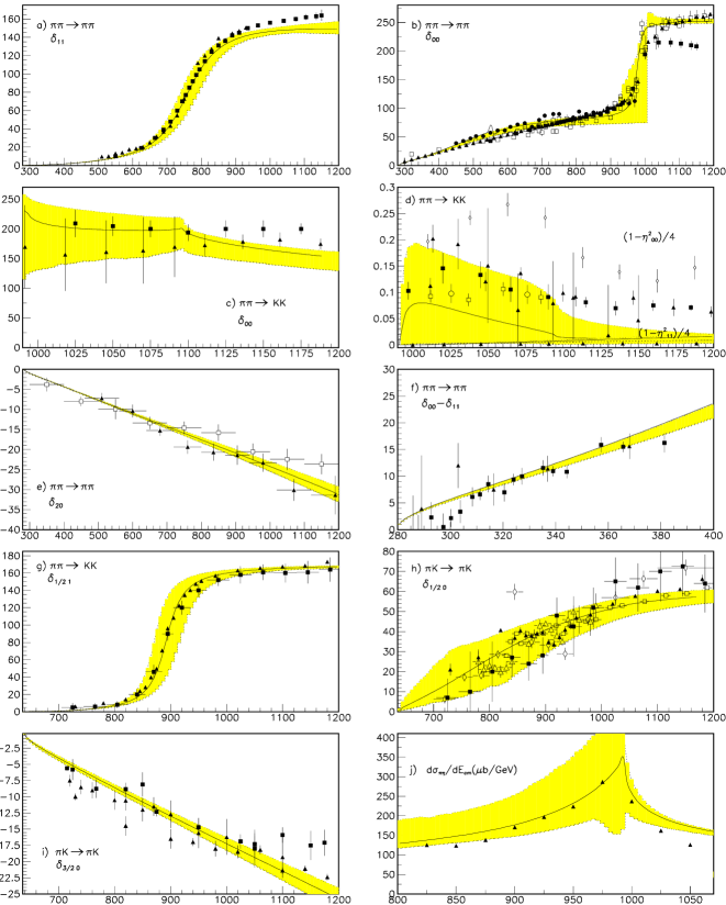
Figure 2: IAM fit to meson-meson scattering data, set II. The uncertainties cover also the estimated systematic errors. The statistical errors from the fit would be much smaller.

We have even performed a third fit, the IAM III, by fixing $L_{4}$ to zero as in the most recent $K_{l4}$ $O(p^{4})$ determinations given also in Table 1.

Let us recall that in these proceedings we are still showing some preliminary results whose calculation is still in progress prep . In a forthcoming work prep we will provide the final numbers (mostly for the errors) and the threshold parameters for these other fits. Concerning the threshold parameters we do not expect relevant changes compared to data since the $\pi\pi\rightarrow\pi\pi$ amplitude has not changed and therefore the new numbers will remain almost identical to those of IAM I.

As we can see in Fig.2, we obtain again a nice description of meson-meson data up to 1.2 GeV, including once more all the resonant behaviors. One may wonder what would be the effect of applying the IAM to higher orders. Only the $\pi\pi\rightarrow\pi\pi$ amplitude has been calculated up to $O(p^{6})$ and it has been unitarized in Nieves:2001de , using the higher order form of IAM. The results regarding poles and resonances in the single channel case are unchanged and the parameters are compatible with those of standard ChPT at $O(p^{6})$.

Finally, let us remark that the IAM has also been applied to $\pi\pi$ elastic scattering in the $(I,J)=(0,2)$ wave Dobado:2001rv , whose leading order vanishes. The amplitude has to be considered up to $O(p^{6})$ and add an approximation at $O(p^{8})$, but the IAM is able to generate a pole associated to the $f_{2}(1200)$ BW resonance. The mass and widths are in fairly good agreement with data taking into account that that resonance has only an 80% decay into pions.

7 Poles in meson-meson scattering

In Table 3 we present the position of poles in the second Riemann sheet of meson-meson scattering calculated with the one-loop IAM. The names we provide refer to the most similar states that we have found in the literature, but that does not mean that from the present approach we could drag any conclusion on their nature. In Table 4 we provide either the mass and width of these resonances or their pole position as given in the PDG.

$\sqrt{s_{pole}}$(MeV)	$\rho$	$K^{*}$	$\sigma$	$f_{0}$	$a_{0}$	$\kappa$
${}^{\hbox{IAM Approx}}_{\;\;\;\hbox{(no errors)}}$	759-i 71	892-i 21	442-i 227	994-i 14	1055-i 21	770-i 250
IAM I	760-i 82	886-i 21	443-i 217	988-i 4	cusp?	750-i 226
(errors)	$\pm$ 52$\pm$ i 25	$\pm$ 50$\pm$ i 8	$\pm$ 17$\pm$ i 12	$\pm$ 19$\pm$ i 3		$\pm$18$\pm$i 11
IAM II	754-i 74	889-i 24	440-i 212	973-i 11	1117-i 12	753-i 235
(errors)	$\pm$ 18$\pm$ i 10	$\pm$ 13$\pm$ i 4	$\pm$ 8$\pm$ i 15	${}^{+39}_{-127}$ ${}^{+i\,189}_{-i\,11}$	${}^{+24}_{-320}$ ${}^{+i\,43}_{-i\,12}$	$\pm$ 52$\pm$ i 33
IAM III	748-i68	889-i23	440-i216	972-i8	1091-i52	754-i230
(errors)	$\pm$ 31$\pm$ i 29	$\pm$ 22$\pm$ i 8	$\pm$ 7$\pm$ i 18	${}^{+21}_{-56}$$\pm$ i 7	${}^{+19}_{-45}$ ${}^{+i\,21}_{-i\,40}$	$\pm$ 22$\pm$ i 27

Table 3: Pole positions (with errors) in meson-meson scattering. When close to the real axis the mass and width of the associated resonance is $\sqrt{s_{pole}}\simeq M-i\Gamma/2$.

PDG2002	$\rho(770)$	$K^{*}(892)^{\pm}$	$\sigma$ or $f_{0}(600)$	$f_{0}(980)$	$a_{0}(980)$	$\kappa$
Mass (MeV)	$771\pm 0.7$	$891.66\pm 0.26$	(400-1200)-i (300-500)	$980\pm 10$	$980\pm 10$	not
Width (MeV)	$149\pm 0.9$	$50.8\pm 0.9$	(we list the pole)	40-100	50-100	listed

Table 4: Mass and widths or pole positions of the light resonances quoted in the PDG. Recall that for narrow resonances $\sqrt{s_{pole}}\simeq M-i\Gamma/2$

Let us briefly comment Table 3. In the first line we are giving the results already obtained in Oller:1997ng , with the approximated coupled channel IAM, using amplitudes with $f_{\pi}$, $f_{K}$ and $f_{\eta}$. It can be noticed that there were nine scalar poles, the $\sigma$, the $f_{0}(980)$, the three states of the $a_{0}(980)$ as well as the four states of the $\kappa$. Since they were generated simultaneously, they could be a good candidate for a nonet, although clearly some mechanism should be producing the mass difference, very likely some kind of mixing with higher order states Oller:1998zr .

Concerning the results of the IAM, we see that there are always poles associated to the vector resonances $\rho$ and $K^{*}$, in good agreement with the data and with the approximated method. The uncertainties in the pole positions have been obtained again using a MonteCarlo Gaussian sample (300 samples) of the $L_{i}$ parameters, within the errors of each set. Let us note that the vector octet is complete, since we also obtain a pole in the $(I,J)=(0,1)$ below the $\bar{K}K$ threshold, but it is only a crude approximation to the $\Phi$ and $\omega$ states (it is the octet $\Phi$ indeed). The problem here is that the other relevant coupled channel that separates the $\Phi$ and the $\omega$ is a three pion state, that we cannot implement in the IAM. For details, we refer the reader to Oller:1999ag ; Oller:1997ng ; GomezNicola:2001as .

Concerning scalar states, from Table 3 we see that the results concerning the most controversial ones are consistent and in very good agreement between different IAM sets and also with the approximated IAM. In other words, the results for the $\sigma$ and the $\kappa$ poles are robust within this approach: there are always “light” poles in the $(I,J)=(0,0),(1/2,0)$ channels, and their position is fairly well determined, in round numbers, around $440-i\,215$ MeV for the $\sigma$ and $750-i\,230$ MeV for the $\kappa$. The errors are comparatively small as it can be seen in Table 3.

The situation concerning $f_{0}$ is also rather stable for the mass, which is always around 975 MeV. In contrast, the uncertainty on the width is rather large. In particular, the central value is somewhat small when using set 1 (just one $f_{\pi}$) but in a fairly good agreement with data when considering sets 2 and 3 or the approximated IAM (all of them use $f_{\pi},f_{K}$ and $f_{\eta}$). As we argued before, it was natural to expect that the use of $f_{K}$ and $f_{\eta}$ when dealing with kaons or etas would provide better results.

Finally, the most sensible state seems to be the $a_{0}(980)$ resonance. It can be noticed that it is present as a pole in the second Riemann sheet in sets 2 and 3 as well as in the approximated IAM. However, it is not found as a pole with set 1, using just $f_{\pi}$. The fact that the $a_{0}(980)$ pole was absent if one uses only the tree level terms and the tadpoles of the complete amplitudes in GomezNicola:2001as (again using just $f_{\pi}$) with the approximated IAM was first noted in Uehara:2002nv and has been interpreted as a possible cusp effect.

Given the uncertainty on the $a_{0}(980)$ it is hard to identify it conclusively as a pole or a cusp. However, we think that there is a somewhat stronger support for the pole interpretation, although with a strong threshold distortion: On the one hand, the width of the $f_{0}(980)$, which is closely related to the $a_{0}(980)$, is much better described by the IAM when using several decay constants, which then give a pole for the $a_{0}(980)$. On the other hand the existence of the $a_{0}(980)$ state seems much less controversial from other sources apart from meson-scattering data PDG . We remark, anyway, that the two possibilities can be accommodated within the IAM.

8 Conclusions

We have reported on our recent work where we have completed the meson-meson scattering amplitudes to one-loop within Chiral Perturbation Theory (ChPT). In order to extend the applicability of these amplitudes to the resonance region, we have unitarized them with the Inverse Amplitude Method (IAM). In this way, we have been able to describe the meson-meson scattering data up to 1.2 GeV, generating the resonant behaviors, but simultaneously respecting the chiral low energy expansion. These new amplitudes are unitarized in dimensional regularization in order to preserve chiral symmetry, avoiding the use of a cutoff. Thus we have been able to check that the chiral parameters obtained from the IAM description are compatible with previous determinations from other processes within standard ChPT.

In this workshop we have also shown our progress in determining the position of the poles that appear in the IAM amplitudes. When they are close to the real axis above threshold, the position of these poles is related to the mass and width of the associated narrow BW resonances.

In this way, we have been able to establish more robustly our results for the controversial $\sigma$ and $\kappa$ scalar states. They seem to be generated simultaneously with the $f_{0}(980)$ and the $a_{0}(980)$, and are therefore good candidates for a possible light scalar nonet. Nevertheless, the $a_{0}(980)$ is found to be very sensible to the choice on how to express the amplitudes in terms of the physical meson decay constants.

We hope these results could be of interest in the field of meson spectroscopy

References

- (1) A. Gómez Nicola and J. R. Peláez, in preparation.
- (2) A. Gómez Nicola and J. R. Peláez, Phys. Rev. D 65 (2002) 054009
- (3) R. Kaminski, L. Lesniak and J. P. Maillet, Phys. Rev. D 50 (1994) 3145. R. Delbourgo and M. D. Scadron, Mod. Phys. Lett. A 10 (1995) 251. S. Ishida et al., Prog. Theor. Phys. 95 (1996) 745. M. Harada, F. Sannino and J. Schechter, Phys. Rev. D 54 (1996) 1991 N. A. Tornqvist and M. Roos, Phys. Rev. Lett. 76 (1996) 1575.
- (4) A. Dobado and J. R. Pelaez, Phys. Rev. D 47 (1993) 4883. Phys. Rev. D 56 (1997) 3057.
- (5) K. Hagiwara et al., Phys. Rev. D 66, 010001 (2002).
- (6) R.L. Jaffe, Phys. Rev. D15 267 (1977); Phys. Rev. D15, 281 (1977). E. van Beveren et al. Z. Phys. C30, 615 (1986). S. Ishida et al, Prog. Theor. Phys. 98,621 (1997). D. Black, A. H. Fariborz, F. Sannino, J. Schechter. Phys. Rev. D58:054012,1998. E. van Beveren and G. Rupp, Eur. Phys. J. C 22 (2001) 493
- (7) J. A. Oller, E. Oset and J. R. Pelaez, Phys. Rev. Lett. 80 (1998) 3452; Phys. Rev. D 59 (1999) 074001 [Erratum-ibid. D 60 (1999) 099906].
- (8) E. van Beveren and G. Rupp, arXiv:hep-ph/0201006.
- (9) S. D. Protopopescu et al., Phys. Rev. D7, (1973) 1279; P. Estabrooks and A.D.Martin, Nucl.Phys.B79, (1974) 301. G. Grayer et al., Nucl. Phys. B75, (1974) 189. D. Cohen, Phys. Rev. D22, (1980) 2595. W. Hoogland et al., Nucl. Phys. B126 (1977) 109. M. J. Losty et al., Nucl. Phys. B69 (1974) 185. R. Mercer et al., Nucl. Phys. B32 (1971) 381. P. Estabrooks et al., Nucl. Phys. B133 (1978) 490. H. H. Bingham et al., Nucl. Phys. B41 (1972) 1. S. L. Baker et al., Nucl. Phys. B99 (1975) 211. D. Aston et al. Nucl. Phys. B296 (1988) 493. D. Linglin et al., Nucl. Phys. B57 (1973) 64 .
- (10) S. Pislak et al. [BNL-E865 Collaboration], Phys. Rev. Lett. 87 (2001) 221801.
- (11) E791 Collaboration, Phys. Rev. Lett. 86,(2001) 770. C. Gobel for the E791 Collab. hep-ex/0012009.
- (12) J. Gasser and H. Leutwyler, Annals Phys. 158 (1984) 142. Nucl. Phys. B 250 (1985) 465.
- (13) T. N. Truong, Phys. Rev. Lett. 61 (1988) 2526. Phys. Rev. Lett. 67, (1991) 2260; A. Dobado, M.J.Herrero and T.N. Truong, Phys. Lett. B235 (1990) 134.
- (14) F. Guerrero and J. A. Oller, Nucl. Phys. B 537 (1999) 459 [Erratum-ibid. B 602 (2001) 641].
- (15) S. Weinberg, Physica A96 (1979) 327.
- (16) V. Bernard, N. Kaiser, U.G. Meissner, Phys. Rev. D43 (1991) 2757; Nucl. Phys. B357 (1991) 129; Phys. Rev. D44 (1991) 3698.
- (17) J. Nieves, M. Pavon Valderrama and E. Ruiz Arriola, Phys. Rev. D 65 (2002) 036002.
- (18) A. Dobado and J. R. Pelaez, Phys. Rev. D 65 (2002) 077502.
- (19) J. A. Oller, E. Oset and J. R. Peláez, Phys. Rev. D 62 (2000) 114017.
- (20) F. James, Minuit Reference Manual D506 (1994).
- (21) G. Amorós, J. Bijnens and P. Talavera, Nucl. Phys. B602 (2001) 87.
- (22) J. Bijnens, G. Colangelo and J. Gasser, Nucl. Phys. B427 (1994) 427.
- (23) G. Amoros, J. Bijnens and P. Talavera, Nucl. Phys. B 585 (2000) 293 [Erratum-ibid. B 598 (2001) 665].
- (24) J. A. Oller and E. Oset, Phys. Rev. D 60 (1999) 074023.
- (25) M. Uehara, arXiv:hep-ph/0204020.