Phenomenology of the Little Higgs Model

Abstract

We study the low energy phenomenology of the little Higgs model. We first discuss the linearized effective theory of the “littlest Higgs model” and study the low energy constraints on the model parameters. We identify sources of the corrections to low energy observables, discuss model-dependent arbitrariness, and outline some possible directions of extensions of the model in order to evade the precision electroweak constraints. We then explore the characteristic signatures to test the model in the current and future collider experiments. We find that the LHC has great potential to discover the new $SU(2)$ gauge bosons and the possible new $U(1)$ gauge boson to the multi-TeV mass scale. Other states such as the colored vector-like quark $T$ and doubly-charged Higgs boson $\Phi^{++}$ may also provide interesting signals. At a linear collider, precision measurements on the triple gauge boson couplings could be sensitive to the new physics scale of a few TeV. We provide a comprehensive list of the linearized interactions and vertices for the littlest Higgs model in the appendices.

I Introduction

One of the major motivations for physics beyond the Standard Model (SM) is to resolve the hierarchy and fine-tuning problems between the electroweak scale and the Planck scale. Supersymmetric theories introduce an extended space-time symmetry and quadratically divergent quantum corrections are canceled due to the symmetry between the bosonic and fermionic partners. This naturally stabilizes the electroweak scale against the large corrections in the ultra-violet (UV) regime. Technicolor theories introduce new strong dynamics at scales not much above the electroweak scale, thus defer the hierarchy problem. Theories with TeV scale quantum gravity reinterpret the problem completely by lowering the fundamental Planck scale. Current and future collider experiments will provide hints to tell us which may be the ultimately correct path.

Recently, there has been a new formulation for the physics of electroweak symmetry breaking, dubbed the “little Higgs” models [1, 2, 3, 4, 5, 6]. The key ideas of the little Higgs theory may be summarized by the following points:

• The Higgs fields are Goldstone bosons [7, 8, 9, 13, 10, 11, 12], associated with some global symmetry breaking at a higher scale $\Lambda_{S}$;

• The Higgs fields acquire a mass and become pseudo-Goldstone bosons via symmetry breaking (possibly radiatively) at the electroweak scale;

• The Higgs fields remain light, being protected by the approximate global symmetry and free from 1-loop quadratic sensitivity to the cutoff scale $\Lambda_{S}$.

The scalar mass in a generic quantum field theory will receive quadratically divergent radiative corrections all the way up to the cut-off scale. The little Higgs model solves this problem by eliminating the lowest order contributions via the presence of a partially broken global symmetry. The non-linear transformation of the Higgs fields under this global symmetry prohibits the existence of a Higgs mass term of the form $m^{2}|h|^{2}$. This can also be illustrated in a more intuitive way: Besides the Standard Model gauge bosons, there are a set of heavy gauge bosons with the same gauge quantum numbers. The gauge couplings to the Higgs bosons are patterned in such a way that the quadratic divergence induced by the SM gauge boson loops are canceled by the quadratic divergence induced by the heavy gauge bosons at one loop level. One also introduces a heavy fermionic state which couples to the Higgs field in a specific way, so that the 1-loop quadratic divergence induced by the top-quark Yukawa coupling to the Higgs boson is canceled. Furthermore, extra Higgs fields exist as the Goldstone boson multiplets from the global symmetry breaking.

It is interesting to note that, unlike the supersymmetry relations between the bosons and fermions, the cancellations of the quadratic divergence in the little Higgs model occur between particles with the same statistics: divergences due to gauge bosons are canceled by new gauge bosons and similarly for the heavy quarks. A scale less than several TeV and the specification of the couplings to the Higgs boson are necessary requirements for the model to avoid fine-tuning. These features could lead to distinctive experimental signatures, which is the subject for the current work. The paper is organized as follows. In Sec. II, we lay out a concrete model as proposed in [4]. We linearize the theory and discuss the important features. In Sec. III, we explore the characteristic phenomenology of this model. Regarding the constraints from the precision electroweak data, we explore the properties associated with the custodial $SU(2)$ breaking and the sources which lead to the large corrections to low-energy observables in the model. We identify the arbitrariness in particular related to the $U(1)$ sector. We then outline the possible fine-tunings or directions of extensions of the model in order to evade the precision electroweak constraints. We also study the characteristic signals at the future collider experiments at the LHC and a linear collider. We summarize our results in Sec. IV. We present the detailed derivation and the Feynman rules of the littlest Higgs model in two appendices.

II The Framework of the Littlest Higgs Model

An explicit model has been constructed based on the idea of the little Higgs models, dubbed the “littlest Higgs model” [4]. It begins with $SU(5)$ global symmetry, with a locally gauged subgroup $G_{1}\otimes G_{2}=[SU(2)_{1}\otimes U(1)_{1}]\otimes[SU(2)_{2}\otimes U(1)_{2}]$. The phase transitions associated with the symmetry breaking in this model proceed in two stages:

1. At scale $\Lambda_{S}$, the global symmetry $SU(5)$ is spontaneously broken down to its subgroup $SO(5)$ via a vev of order $f$. Naive Dimensional Analysis [14, 15, 16] establishes a simple relation $\Lambda_{S}\sim 4\pi f$. At the same time, the gauge symmetry $[SU(2)\otimes U(1)]^{2}$ is also broken into its diagonal subgroup $SU(2)_{L}\otimes U(1)_{Y}$, identified as the SM gauge group. The global symmetry breaking leaves 14 massless Goldstone bosons which transform under the electroweak gauge group as a real singlet ${\mathbf{1}}_{0}$, a real triplet ${\mathbf{3}}_{0}$, a complex doublet ${\mathbf{2}}_{\pm\frac{1}{2}}$, and a complex triplet ${\mathbf{3}}_{\pm 1}$. The real singlet and the real triplet become the longitudinal components of the gauge bosons associated with the broken gauge groups, giving them masses of the order $f$, while the complex doublet and the complex triplet remain massless at this stage.

2. The presence of gauge and Yukawa couplings that break the global $SO(5)$ symmetry will induce a Coleman-Weinberg [17] type potential for the remaining pseudo-Goldstone bosons. In particular, it will give the complex triplet a heavy mass of the order $f$ and give the neutral component of the complex doublet a non-vanishing vacuum expectation value (vev) $v$ which in turn triggers the electroweak symmetry breaking.

Before we lay out the effective field theory below the scale of $\Lambda_{S}$ for the littlest Higgs model, we note that some matching procedure for the operators that are sensitive to physics at higher energies will eventually be needed. Namely, one would need to consider the UV origin of the theory above $\Lambda_{S}$. We will not attempt to explore the UV completion of the theory in this paper but rather refer the reader to some discussions in the literature [4, 18].

II.1 Scalar and Gauge Boson Sector

II.1.1 Gauge Bosons and Pseudo-Goldstone Bosons

At the scale $\Lambda_{S}$, a vev $f$ breaks the assumed global $SU(5)$ symmetry into its subgroup $SO(5)$, resulting in 14 Goldstone bosons. The effective field theory of those Goldstone bosons is parameterized by a non-linear $\sigma$-model with a gauge symmetry $[SU(2)\otimes U(1)]^{2}$, spontaneously broken down to the Standard Model gauge group. In particular, the Lagrangian will still preserve the full $[SU(2)\otimes U(1)]^{2}$ gauge symmetry. The leading order dimension-two term in the non-linear $\sigma$-model can be written for the scalar sector as [4]

$$\mathcal{L}_{\Sigma}=\frac{1}{2}\frac{f^{2}}{4}{\rm Tr}|\mathcal{D}_{\mu}\Sigma|^{2}.$$ (1)

The numerical coefficients have been chosen so that the scalar kinetic terms are canonically normalized. The covariant derivative is defined as

$$\mathcal{D}_{\mu}\Sigma=\partial_{\mu}\Sigma-i\sum_{j=1}^{2}\left(g_{j}(W_{j}\Sigma+\Sigma W_{j}^{T})+g^{\prime}_{j}(B_{j}\Sigma+\Sigma B_{j}^{T})\right).$$ (2)

To linearize the theory, one can expand $\Sigma$ in powers of ${1}/{f}$ around its vacuum expectation value $\Sigma_{0}$

$$\Sigma=\Sigma_{0}+\frac{2i}{f}\left(\begin{array}[]{ccccc}\phi^{\dagger}&\frac{h^{\dagger}}{\sqrt{2}}&{\mathbf{0}}_{2\times 2}\\ \frac{h^{*}}{\sqrt{2}}&0&\frac{h}{\sqrt{2}}\\ {\mathbf{0}}_{2\times 2}&\frac{h^{T}}{\sqrt{2}}&\phi\end{array}\right)+{\cal O}(\frac{1}{f^{2}}),$$ (3)

where $h$ is a doublet and $\phi$ is a triplet under the unbroken $SU(2)$. The appearance of the $\Sigma_{0}$ breaks the local gauge symmetry $[SU(2)\otimes U(1)]^{2}$ into its diagonal subgroup $[SU(2)\otimes U(1)]_{SM}$, giving rise to mass of order $f$ for half of the gauge bosons

$$m_{W^{\prime}}=\frac{f}{2}\sqrt{g_{1}^{2}+g_{2}^{2}}=\frac{g}{2sc}f,\qquad m_{B^{\prime}}=\frac{f}{2\sqrt{5}}\sqrt{g_{1}^{\prime 2}+g_{2}^{\prime 2}}=\frac{g^{\prime}}{2\sqrt{5}s^{\prime}c^{\prime}}f,$$ (4)

with the field rotation to the mass eigenstates given by

$$W=sW_{1}+cW_{2}, W^{\prime}=-cW_{1}+sW_{2}$$

$$B=s^{\prime}B_{1}+c^{\prime}B_{2}, B^{\prime}=-c^{\prime}B_{1}+s^{\prime}B_{2}.$$ (5)

The mixing angles are given by

$$s=\frac{g_{2}}{\sqrt{g_{1}^{2}+g_{2}^{2}}},\qquad s^{\prime}=\frac{g_{2}^{\prime}}{\sqrt{g_{1}^{\prime 2}+g_{2}^{\prime 2}}}.$$ (6)

The $W$ and $B$ remain massless and are identified as the SM gauge bosons, with couplings

$$g=g_{1}s=g_{2}c,\qquad g^{\prime}=g_{1}^{\prime}s^{\prime}=g_{2}^{\prime}c^{\prime}.$$ (7)

The couplings of $W$, $W^{\prime}$ to two scalars are given by:

$$\mathcal{L}_{\Sigma}(W\cdot W) = \frac{g^{2}}{4}\left[W^{a}_{\mu}W^{b\mu}-\frac{(c^{2}-s^{2})}{sc}W^{a}_{\mu}W^{\prime b\mu}\right]{\rm Tr}\left[h^{\dagger}h\delta^{ab}+2\phi^{\dagger}\phi\delta^{ab}+2\sigma^{a}\phi^{\dagger}\sigma^{bT}\phi\right]$$ (8)

$$- \frac{g^{2}}{4}\left[W^{\prime a}_{\mu}W^{\prime a\mu}{\rm Tr}\left[h^{\dagger}h+2\phi^{\dagger}\phi\right]-\frac{(c^{4}+s^{4})}{2s^{2}c^{2}}W^{\prime a}_{\mu}W^{\prime b\mu}{\rm Tr}\left[2\sigma^{a}\phi^{\dagger}\sigma^{bT}\phi\right]\right].$$

In the SM, the four-point couplings of the form $WWh^{\dagger}h$ lead to a quadratically divergent contribution to the Higgs mass. In the littlest Higgs model, however, the $W^{\prime}W^{\prime}h^{\dagger}h$ coupling has an unusual form as seen in Eq. (8), which serves to exactly cancel the quadratic divergence in the Higgs mass arising from the seagull diagram involving a $W$ boson loop. Similarly, the couplings of $B$, $B^{\prime}$ to two scalars are:

$$\mathcal{L}_{\Sigma}(B\cdot B) = g^{\prime 2}\left[B_{\mu}B^{\mu}-\frac{(c^{\prime 2}-s^{\prime 2})}{s^{\prime}c^{\prime}}B_{\mu}B^{\prime\mu}\right]{\rm Tr}\left[\frac{1}{4}h^{\dagger}h+\phi^{\dagger}\phi\right]$$ (9)

$$- g^{\prime 2}\left[B_{\mu}^{\prime}B^{\prime\mu}{\rm Tr}\left[\frac{1}{4}h^{\dagger}h\right]-\frac{(c^{\prime 2}-s^{\prime 2})^{2}}{4s^{\prime 2}c^{\prime 2}}B_{\mu}^{\prime}B^{\prime\mu}{\rm Tr}\left[\phi^{\dagger}\phi\right]\right].$$

We see that the $B^{\prime}B^{\prime}$ coupling to $h^{\dagger}h$ serves to exactly cancel the quadratic divergence in the Higgs mass arising from the seagull diagram involving a $B$ boson loop. Note that terms of the form $W\partial hh$ would not produce a quadratic divergence by power counting. This absence of the quadratically divergent Higgs mass term at one-loop order can also be understood by a set of global symmetries under which the Higgs doublet transforms non-linearly and which is preserved partially by the various interactions in the effective Lagrangian at scale $\Lambda_{S}$ [4].

This cancellation may not follow one’s intuition at first sight. It turns out that the appearance of the different sign between the two $SU(2)^{\prime}$s (or $U(1)^{\prime}$s) can be traced back to the unique pattern of gauge symmetry breaking. For instance, the broken generators (associated with $W^{\prime}$) are

$$Q^{\prime a}=\frac{1}{\sqrt{g_{1}^{4}+g_{2}^{4}}}(g_{1}^{2}Q_{1}^{a}-g_{2}^{2}Q_{2}^{a}),$$ (10)

which do not satisfy the standard $SU(2)$ commutation relations. Technically, this is the reason for the unusual negative sign of the gauge couplings of the Higgs boson to $W^{\prime}$ ($B^{\prime}$).

II.1.2 Higgs Bosons and the Electroweak Symmetry Breaking

The electroweak symmetry breaking in this model is triggered by the Higgs potential generated by one-loop radiative corrections. The Higgs potential includes the parts generated by the gauge boson loops as well as the fermion loops. They can be presented in the standard form of the Coleman-Weinberg potential in terms of $M_{V}^{2}(\Sigma)$ and $M_{f}^{2}(\Sigma)$. By expanding the nonlinear $\sigma$-model field $\Sigma$ as usual, we obtain the Higgs potential

$$V=\lambda_{\phi^{2}}f^{2}{\rm Tr}(\phi^{\dagger}\phi)+i\lambda_{h\phi h}f\left(h\phi^{\dagger}h^{T}-h^{*}\phi h^{\dagger}\right)-\mu^{2}hh^{\dagger}+\lambda_{h^{4}}(hh^{\dagger})^{2},$$ (11)

where the coefficients $\lambda_{\phi^{2}}$, $\lambda_{h\phi h}$, and $\lambda_{h^{4}}$ are functions of the fundamental parameters in this model (the gauge couplings, top-quark Yukawa coupling, and two new coefficients $a,a^{\prime}$ in the Coleman-Weinberg potential), as explicitly given in Eq. (79) in the appendix. There could exist important two-loop contributions to the Higgs potential. A term like $\Lambda_{S}^{2}h^{2}/(16\pi^{2})^{2}\sim f^{2}h^{2}/(16\pi^{2})$ gives rise to a mass term for $hh^{\dagger}$ which could be as large as the one-loop Coleman-Weinberg potential contribution. We will not attempt to evaluate these two-loop contributions explicitly in terms of model parameters. Instead, the Higgs mass parameter $\mu^{2}$ should be treated as a new free parameter of the order of $f^{2}/16\pi^{2}$.

Minimizing the potential to obtain the doublet and triplet vevs $v$ and $v^{\prime}$, it is easy to arrive at a relation (see the Appendix for details):

$$\frac{\lambda_{h\phi h}}{\lambda_{h^{4}}}=\frac{4\lambda_{h\phi h}}{\lambda_{\phi^{2}}}=\frac{8v^{\prime}}{v}\frac{f}{v}.$$ (12)

Diagonalizing the Higgs mass matrix, we obtain Higgs masses to the leading order

$$M^{2}_{\Phi}\simeq\lambda_{\phi^{2}}f^{2},\qquad m^{2}_{H}\simeq 2\left(\lambda_{h^{4}}-\lambda_{h\phi h}^{2}/\lambda_{\phi^{2}}\right)v^{2}=2\mu^{2}.$$ (13)

Note that we must have $\lambda_{\phi^{2}}>0$ to avoid generating a triplet vev of order $f$, in gross violation of experimental constraints. Also, we must have $\lambda_{h^{4}}>\lambda_{h\phi h}^{2}/\lambda_{\phi^{2}}$ in order to get the correct vacuum for the electro-weak symmetry breaking (EWSB) with $m^{2}_{H}>0$. The masses of the triplet states are degenerate at this order. We can further relate the masses by

$$M^{2}_{\Phi}=\frac{2m_{H}^{2}f^{2}}{v^{2}}\frac{1}{\left[1-(4v^{\prime}f/v^{2})^{2}\right]}.$$ (14)

We can thus express all four parameters in the Higgs potential, to leading order, in terms of the physical parameters $f$, $m_{H}^{2}$, $v$, and $v^{\prime}$. As a side product, we obtain a relation among the vevs by demanding the triplet mass squared to be positive definite

$${v^{\prime 2}\over v^{2}}<{v^{2}\over 16f^{2}}.$$ (15)

It is informative to note that the couplings of the Higgs triplet to the massive gauge bosons are relatively suppressed by $v^{\prime}/v$; while the charged Higgs boson couplings to a photon are of the full electromagnetic strength.

Now let us estimate the naturalness bound on the scale $f$ for keeping $m_{H}$ light. We have the generic expression for

$$m^{2}_{H}=2\mu^{2}\simeq a_{{\text{1-loop}}}\frac{f^{2}}{16\pi^{2}}+a_{{\text{2-loop}}}\frac{f^{2}}{16\pi^{2}},$$ (16)

with both $a_{{\text{1-loop}}}$ (we have absorbed a factor of $\log(16\pi^{2})$ into the definition of $a_{{\text{1-loop}}}$ ) and $a_{{\text{2-loop}}}$ containing many contributions (terms) from different interactions. Assuming that there is no large cancellation and $m_{H}^{2}$ is no less than $10\%$ of the magnitude of the largest term on the right-hand side of Eq. (16), we obtain a rough estimate of the natural scale

$$f\leq\frac{4\pi m_{H}}{\sqrt{0.1a_{\rm max}}}\simeq\frac{8\ {\rm TeV}}{\sqrt{a_{\rm max}}}\left(\frac{m_{H}}{200\ {\rm GeV}}\right),$$ (17)

where $a_{\text{max}}$ denotes the largest coefficient of the terms in Eq. (16) which could be of the order of 10.

II.1.3 Gauge Boson Mass Eigenstates

The EWSB induces further mixing between the light and heavy gauge bosons. The final mass eigenstates for the charged gauge bosons are $W_{L}$ (light) and $W_{H}$ (heavy), with masses to the order of $v^{2}/f^{2}$ given by

$$M_{W_{L}^{\pm}}^{2} = m_{w}^{2}\left[1-\frac{v^{2}}{f^{2}}\left(\frac{1}{6}+\frac{1}{4}(c^{2}-s^{2})^{2}\right)+4\frac{v^{\prime 2}}{v^{2}}\right],$$ (18)

$$M_{W_{H}^{\pm}}^{2} = m_{w}^{2}\left(\frac{f^{2}}{s^{2}c^{2}v^{2}}-1\right),$$ (19)

where the mass parameter $m_{w}\equiv gv/2$ approaches the SM $W$-boson mass when $f\to\infty$. Note that the $W_{L}$ mass gets a correction at order $v^{2}/f^{2}$, which will modify the relation among the $W$ mass, $g$, and $G_{F}$. The neutral gauge boson masses are similarly given by

$$M_{A_{L}}^{2} = 0,$$

$$M_{Z_{L}}^{2} = {m_{z}^{2}}\left[1-\frac{v^{2}}{f^{2}}\left(\frac{1}{6}+\frac{1}{4}(c^{2}-s^{2})^{2}+\frac{5}{4}(c^{\prime 2}-s^{\prime 2})^{2}\right)+8\frac{v^{\prime 2}}{v^{2}}\right],$$ (20)

$$M_{A_{H}}^{2} = m_{z}^{2}s_{\rm w}^{2}\left(\frac{f^{2}}{5s^{\prime 2}c^{\prime 2}v^{2}}-1+\frac{x_{H}c_{\rm w}^{2}}{4s^{2}c^{2}s_{\rm w}^{2}}\right)$$ (21)

$$M_{Z_{H}}^{2} = m_{w}^{2}\left(\frac{f^{2}}{s^{2}c^{2}v^{2}}-1-\frac{x_{H}s_{\rm w}^{2}}{s^{\prime 2}c^{\prime 2}c_{\rm w}^{2}}\right),$$ (22)

where $m_{z}\equiv{gv}/(2c_{\rm w})$ is the SM limit when $f\to\infty$. Again, the $Z_{L}$ mass gets a correction at order $v^{2}/f^{2}$. $x_{H}$ characterizes the heavy gauge boson mixing and depends on the gauge couplings as given in the appendix.

The ratio of the $W_{L}$ and $Z_{L}$ boson masses (which are identified as those experimentally observed), to order $v^{2}/f^{2}$, is:

$$\frac{M_{W_{L}^{\pm}}^{2}}{M_{Z_{L}}^{2}}=c_{\rm w}^{2}\left[1+\frac{v^{2}}{f^{2}}\frac{5}{4}(c^{\prime 2}-s^{\prime 2})^{2}-4\frac{v^{\prime 2}}{v^{2}}\right].$$ (23)

The breaking of the custodial $SU(2)$ symmetry at order $v^{2}/f^{2}$ in this model is manifest. The tree-level SM relation $M_{W}^{2}/M_{Z}^{2}=c^{2}_{\rm w}$ (or $\rho=1$) is no longer valid. This breaking of the custodial $SU(2)$ symmetry can be traced back to the vacuum expectation value of $\Sigma$. As shown in Eq. (62), the $\mathcal{O}(1/f^{2})$ term in the expansion has its $h^{\dagger}h$ vev in the position of the neutral component of the scalar triplet in the $\mathcal{O}(1/f)$ term in the expansion. Thus the $h$ vev acts like a triplet vev at order $v^{2}/f^{2}$. The $U(1)$ gauge coupling of the triplet also breaks the custodial $SU(2)$ at the order $v^{\prime 2}/v^{2}$. It is also interesting to note that for the case of no mixing $s^{\prime}=c^{\prime}$ (or $g_{1}^{\prime}=g_{2}^{\prime}$) and $v^{\prime}=0$, the $W,Z$ mass ratio remains the SM form. We will discuss the theoretical origin of the custodial $SU(2)$ symmetry breaking in more detail in Sec. II.3.

II.2 Fermions and Their Interactions

II.2.1 Yukawa Interactions

The Standard Model fermions acquire their masses through the Higgs mechanism via Yukawa interactions. Due to its large Yukawa coupling to the Higgs field, the top quark introduces a quadratic correction to the Higgs boson mass of the order ${y_{t}^{2}}\Lambda_{S}^{2}/(16\pi^{2})\sim f^{2}$ and spoils the naturalness of a light Higgs boson. In the littlest Higgs model [4], this problem is resolved by introducing a new set of heavy fermions with couplings to the Higgs field such that it cancels the quadratic divergence due to the top quark. The new fermions come in as a vector-like pair, $\tilde{t}$ and $\tilde{t}^{\prime c}$, with quantum numbers $({\mathbf{3,1}})_{Y_{i}}$ and $({\mathbf{\bar{3},1}})_{-Y_{i}}$. Therefore, they are allowed to have a bare mass term which is chosen to be of order $f$. The coupling of the Standard Model top quark to the pseudo-Goldstone bosons and the heavy vector pair in the littlest Higgs model is chosen to be

$${\mathcal{L}}_{Y}={1\over 2}\lambda_{1}f\epsilon_{ijk}\epsilon_{xy}\chi_{i}\Sigma_{jx}\Sigma_{ky}u^{\prime c}_{3}+\lambda_{2}f\tilde{t}\tilde{t}^{\prime c}+{\rm h.c.},$$ (24)

where $\chi_{i}=(b_{3},t_{3},\tilde{t})$ and $\epsilon_{ijk}$ and $\epsilon_{xy}$ are antisymmetric tensors. It is now straightforward to work out the Higgs-heavy quark interactions, as given in Appendix A.4. The most important consequence is the cancellation of the quadratically divergent corrections to the Higgs mass due to $t_{3},\tilde{t},u^{\prime c}_{3}$ at the one-loop order explicitly seen in Eq. (A.4),

$$-i\lambda_{1}(\sqrt{2}h^{0}t_{3}+if\tilde{t}-\frac{i}{f}h^{0}h^{0*}\tilde{t})u_{3}^{\prime c}+{\rm h.c.}$$

This is due to the flavor (anti)symmetry introduced in Eq. (24). The mass of the vector-like quark is arbitrary in principle. It is chosen by hand as $\lambda_{2}f$ to preserve naturalness. It is a tuning in this sense. However, once we make this choice, it is stable against radiative corrections. The new model-parameters $\lambda_{1},\ \lambda_{2}$ are supposed to be of the order of unity.

Expanding the $\Sigma$ field and diagonalizing the mass matrix, we obtain our physical states $t_{L},\ t_{R}^{c},\ T_{L}$ and $T_{R}^{c}$ with masses

$${\mathcal{L}}_{f}=-m_{t}t_{L}t_{R}^{c}-M_{T}T_{L}T_{R}^{c}$$ (25)

where, up to order $v^{2}/f^{2}$ relative to the leading term,

$$m_{t} = \frac{i\lambda_{1}\lambda_{2}}{\sqrt{\lambda_{1}^{2}+\lambda_{2}^{2}}}v\left\{1+\frac{v^{2}}{f^{2}}\left[-\frac{1}{3}+\frac{fv^{\prime}}{v^{2}}+\frac{1}{2}\frac{\lambda_{1}^{2}}{\lambda_{1}^{2}+\lambda_{2}^{2}}\left(1-\frac{\lambda_{1}^{2}}{\lambda_{1}^{2}+\lambda_{2}^{2}}\right)\right]\right\},$$

$$M_{T} = -f\sqrt{\lambda_{1}^{2}+\lambda_{2}^{2}}\left[1+\mathcal{O}(v^{2}/f^{2})\right].$$ (26)

Since the top-quark mass is already known in the SM, we have the approximate relation

$${1\over\lambda_{1}^{2}}+{1\over\lambda_{2}^{2}}\approx\left({v}\over m_{t}\right)^{2}.$$ (27)

which gives the absolute bounds on the couplings

$${\lambda_{1}}\geq{m_{t}\over v},\quad{\lambda_{2}}\geq{m_{t}\over v},\quad{\rm or}\quad{\lambda_{1}\lambda_{2}}\geq{2}\left({m_{t}}\over v\right)^{2}.$$ (28)

The scalar interactions with the up-type quarks of the first two generations can be chosen to take the same form as in Eq. (24), except that there is no need for the extra vector-like quarks $\tilde{t},\tilde{t}^{\prime c}$. The interactions with the down-type quarks and leptons of the three generations are generated by a similar Lagrangian, as given in Appendix A.4.

We choose the Standard Model fermions to be charged only under $SU(2)_{1}$ with generator $Q_{1}^{a}$. The $SU(2)$ gauge invariance of Eq. (24) is transparent: The first term is actually invariant under an $SU(3)$ rotation under which $\chi_{i}$ transforms like a vector and $\Sigma$ is transformed by a $3\times 3$ unitary rotation embedded in the upper corner of the $5\times 5$ matrix.

	$Q$	$u^{\prime c}$	$d^{c}$	$L$	$e^{c}$	$\tilde{t}$	$\tilde{t}^{\prime c}$
$Y_{1}$	$-\frac{3}{10}-y_{u}$	$y_{u}$	$\frac{3}{5}+y_{u}$	$\frac{3}{10}-y_{e}$	$y_{e}$	$\frac{1}{5}-y_{u}$	$-\frac{1}{5}+y_{u}$
$Y_{2}$	$\frac{7}{15}+y_{u}$	$-\frac{2}{3}-y_{u}$	$-\frac{4}{15}-y_{u}$	$-\frac{4}{5}+y_{e}$	$1-y_{e}$	$\frac{7}{15}+y_{u}$	$-\frac{7}{15}-y_{u}$

Table 1: Fermion $U(1)$ hypercharge assignments required for fermion couplings to scalars to be invariant under $[SU(2)\otimes U(1)]_{1}\otimes[SU(2)\otimes U(1)]_{2}$.

The embedding of the two $U(1)$’s in this model can also be constructed by the gauge invariance of ${\mathcal{L}}_{Y}$. The basic requirement is to reproduce the diagonal $U(1)_{Y}$ as the SM hypercharge

$$Y_{1}+Y_{2}=Y.$$ (29)

Some remarks are in order:

1. The gauge invariance of Eq. (24) under $U(1)_{1}\otimes U(1)_{2}$ dictates the hypercharge assignments of the fermions, which is the major difference between our scheme and those in the literature [19, 20], where the SM fermions are assumed to be charged only under one $U(1)$ gauge group. Giving up the requirement of gauge invariance of $U(1)_{1}\otimes U(1)_{2}$ should be acceptable in principle, for example, by introducing extra fields breaking the $U(1)$’s at a scale $\Lambda_{S}$. However, this is an additional complication of the littlest Higgs model which may need extra arguments for its naturalness.

2. The gauge invariance of Eq. (24) alone cannot unambiguously fix all the $U(1)$ charge values. We list them in Table 1. Two parameters $y_{u}$ and $y_{e}$ are undetermined. They can be fixed by requiring that the $U(1)$ charge assignments be anomaly free, i.e., $Y_{1}=xY,\ Y_{2}=(1-x)Y$. This leads to the particular values

   $$y_{u}=-\frac{2}{5},\hskip 28.45274pty_{e}=\frac{3}{5}.$$ (30)

   However, as an effective field theory below a cutoff, it is unnecessary to be completely anomaly free, although it is certainly a desirable property from a model building point of view since we do not have to introduce specific type of extra matter at the cutoff scale. In this sense, $y_{u}$ and $y_{e}$ can be thought of as partially parameterizing the model dependence of the $U(1)$ sector of some extension of the littlest Higgs model. In our current study, we choose not to be limited by the requirement of anomaly cancellation and indicate the anomaly free assignment as a special case.

3. It is convenient and simple to assume that the first two generations of quarks also obtain their masses through a coupling similar to the first term in Eq. (24). However, this requires some tuning of the parameters to get the correct fermion mass hierarchy. It is certainly no worse than the tuning of the Yukawa couplings in the Standard Model. On the other hand, it might be interesting to postulate that the mass terms of the first two generations actually come from higher dimensional operators of the form $\bar{q}q{\mathcal{O}}/\Lambda^{n}_{S}$, where ${\mathcal{O}}$ is some operator obtaining a vev of mass dimension $(n+1)$. The fields in operator ${\mathcal{O}}$ can have different origins for different generations. Depending on its form and field content, we can again have some relations of the $U(1)$ charge assignments different from the third generation. In particular, if the operator ${\mathcal{O}}$ is composed of the vevs of the pseudo-Goldstone bosons in $\Sigma$, some relations can be derived. However, these relations are much less constrained so that we can effectively treat the hypercharge of the first two generations of fermions as free parameters with the only constraint $Y_{1}+Y_{2}=Y$. If we further impose the anomaly cancellation condition, we can assign only a discrete set of possible values.

With these possibilities in mind, the phenomenological study of the couplings of the $U(1)$ currents may contain large uncertainties due to model-dependence. We choose to study the rather simple case in which all three generations obtain their masses from the same type of gauge invariant operator as the first term in Eq. (24).

II.2.2 Fermion Gauge Interactions

Assuming the fermions transform under $G_{1}\otimes G_{2}$ analogous to the SM, the fermion gauge interactions can be constructed in a standard way, as given in the appendix. The SM weak-boson couplings to fermions receive corrections of the order $v^{2}/f^{2}$, while the electromagnetic coupling remains unchanged, as required by the unbroken electromagnetic gauge interaction. There are new heavy gauge bosons to mediate new gauge interactions.

For the gauge couplings involving the top quark, we must include the mixing between the chiral $t_{3}$ and the vector-like $\tilde{t}$. Since these fermions have different $SU(2)\otimes U(1)$ quantum numbers, their mixing will lead to flavor changing neutral currents mediated by the $Z_{L}$ boson formally at the order of $v/f$. The two right-handed fermions, $u_{3}^{c}$ and $\tilde{t}^{c}$, have the same quantum numbers under the Standard Model $SU(2)\otimes U(1)$ gauge groups, so that their mixing does not cause any FCNC gauge couplings involving the light gauge bosons. A similar argument is applicable to the charged current, which gets modified as

$$J^{+\mu}=\frac{1}{\sqrt{2}}\left[c_{L}\bar{t}_{L}\gamma^{\mu}b_{L}+s_{L}\bar{T}_{L}\gamma^{\mu}b_{L}\right],$$ (31)

where $c_{L}$, $s_{L}$ are given in Eq. (99). It is useful for future phenomenological studies to write the mixing to order $v/f$ as

$$s_{L}\simeq\frac{\lambda_{1}}{\lambda_{2}}\frac{m_{t}}{M_{T}}.$$ (32)

We will also assume that the first two generations get their masses through normal Yukawa couplings which reproduce, to the leading order in $v/f$, the usual CKM matrix. However, because of the mixing of the $SU(2)$ doublet state $t_{3}$ into the heavier mass eigenstate $T_{L}$, the CKM matrix involving only the SM quarks is no longer unitary and the leading deviation occurs at the order $v^{2}/f^{2}$, as given by

$$V_{tb} = c_{L}V_{tb}^{\rm SM}=V_{tb}^{\rm SM}\left(1-\frac{1}{2}\frac{\lambda_{1}^{2}}{\lambda_{2}^{2}}\frac{m_{t}^{2}}{M_{T}^{2}}\right),$$

$$V_{Tb} = s_{L}V_{tb}^{\rm SM}=V_{tb}^{\rm SM}\frac{\lambda_{1}}{\lambda_{2}}\frac{m_{t}}{M_{T}}.$$ (33)

It is apparent from the Feynman rules in Appendix B how the heavy fermion $T$ couples to other particles. $\overline{T_{R}}t_{L}H$ has a coupling of order one (not suppressed by any powers of $v/f$), and the couplings to SM gauge bosons are formally suppressed by $v/f$. However the couplings to the longitudinally polarized gauge bosons gain an enhanced factor $f/v$, resulting in an effective coupling the same strength as that to $H$. We will discuss the phenomenological implications in Sec. III.4.

II.3 On the $SU(2)$ Custodial Symmetry

An immediate question for an extended model is the possible tree-level violation of the $SU(2)$ custodial symmetry and therefore potentially large deviations from the SM prediction for the $\rho$ parameter. We briefly touched upon this issue when we presented the $W,Z$ masses with Eq. (23). We now comment on the general features of little Higgs models in this regard, but will discuss the numerical constraints on the littlest Higgs model and the possible ways to evade the constraints in the next phenomenology section.

It is instructive to compare the littlest Higgs model with the Georgi-Kaplan composite Higgs model [10]. In that model, which also has a global symmetry breaking pattern $SU(5)\rightarrow SO(5)$, only one of the $SU(2)$ symmetries is gauged while the other is used as the $SU(2)$ custodial global symmetry. Therefore, we might expect that the littlest Higgs model, where both of the $SU(2)^{\prime}$s are gauged, will violate the custodial symmetry that protects the tree-level relation of the $W$ and $Z$ masses, and $\rho=1$. The absence of the custodial $SU(2)$ symmetry is indeed true: Within the framework of $SU(5)\rightarrow SO(5)$ and gauging both $SU(2)$ subgroups, it is not possible to have another global custodial $SU(2)$ symmetry.

There are three sources of custodial symmetry violation in this model. First, it is very interesting to note that although the masses of both the SM-like gauge bosons $W$ and $Z$ are shifted due to their mixing with the heavy $SU(2)$ gauge bosons, see e.g. the $c^{2},s^{2}$ terms in Eqs. (18) and (20), the mass ratio still remains unchanged from that in the Standard Model. Therefore, gauging the second $SU(2)$ does not give rise to tree-level corrections to the mass ratio. However, there are indeed some new tree-level contributions to the effective $\rho$ parameter defined through the neutral current couplings, coming from the exchange of the new heavy gauge bosons which in turn induce new four-fermion interactions.

Second, the two $U(1)$’s in the littlest Higgs model violate the custodial symmetry. One combination of them is actually the Standard Model hypercharge so the violation is similar to that in the Standard Model. However, the other combination does introduce new tree-level custodial symmetry violation. It is interesting to compare it with the Georgi-Kaplan model [10], where there is an explicitly conserved $SU(2)$ custodial symmetry broken only by the usual $U(1)_{Y}$. One important difference is that the $U(1)_{A}$ introduced in Ref. [10] to drive the electroweak symmetry breaking is chosen to actually preserve the custodial $SU(2)$ symmetry. Therefore, in their model even radiative corrections from the new $U(1)$ do not introduce new custodial symmetry violation.

Finally, the Higgs triplet coupling to the $SU(2)$ gauge bosons does not have the $SU(2)$ custodial symmetry. However, for the parameter space of this model, the triplet only gets a much smaller vev ($v^{\prime}$) than the doublet and the correction from the triplet in the form of ${v^{\prime 2}}/{v^{2}}$ is smaller than that from the Higgs doublet vev.

We will discuss the implications of the exchange of heavy $SU(2)\otimes U(1)$ gauge bosons and the existence of the triplet vev on the electroweak precision measurements, as well as possible modifications of the littlest Higgs model, in Sec.III.2.1.

III Phenomenology of the littlest Higgs model

We have presented a linearized theory based on the littlest Higgs model [4] and discussed some of its main features. It would be ultimately desirable if some of its qualitative features can be experimentally verified. For this purpose, we explore the phenomenology in this section. We first summarize the model parameters and their relevant ranges. We then discuss the low energy constraints and possible directions of extension of the model to evade the constraints. With the possible and even desirable extensions of the model in mind, we will focus our phenomenological studies on the generic features which will likely be present even in some extensions of the model. The existence of the heavy gauge bosons is generic if the one-loop quadratic divergence is canceled using the little Higgs idea. The presence of the heavy fermions is also a necessary ingredient to control the contribution of the top loop. For a model in which the Higgs doublet is a pseudo-Goldstone boson resulting from a global symmetry breaking, most likely the Higgs sector would not be minimal and extra scalar states will be present.

III.1 Parameters in the Littlest Higgs Model

III.1.1 Couplings

Due to the enlarged gauge group $[SU(2)_{1}\otimes U(1)_{1}]\otimes[SU(2)_{2}\otimes U(1)_{2}]$, there are four gauge couplings $g_{1},\ g_{2},\ g^{\prime}_{1},$ and $g^{\prime}_{2}$. Upon identifying the diagonal part as the SM gauge group, whose couplings are experimentally determined, we obtain the relations:

$${1\over g_{1}^{2}}+{1\over g_{2}^{2}}={1\over g^{2}}\approx{1\over 0.43},\qquad{1\over g_{1}^{\prime 2}}+{1\over g_{2}^{\prime 2}}={1\over g^{\prime 2}}\approx{1\over 0.12},$$ (34)

or equivalently given by Eq. (7).

Top quark and heavy vector-like quark couplings $\lambda_{1}$ and $\lambda_{2}$ are related to give the SM top Yukawa coupling and thereby the correct top-quark mass. This is given by Eq. (27) as

$${1\over\lambda_{1}^{2}}+{1\over\lambda_{2}^{2}}\approx 2.$$ (35)

The proportionality constants $a$ and $a^{\prime}$ in the EWSB sector from the Coleman-Weinberg potential, as discussed in appendix A.2, remain as free parameters. They enter the Higgs potential which determines the Higgs boson masses and their couplings. Their values again depend on the matching condition performed at the scale $\Lambda_{S}$ which in turn depends on the details of the UV completion. Neither the limits on $a$ and $a^{\prime}$ nor the direct measurements of both of them can tell us directly what the UV completion is. However, some numerical knowledge about them will give us very useful hints of the possible structure of the UV theory. As we will discuss later, they can be traded for other physical observable parameters.

III.1.2 Heavy masses

Figure 1: Theoretical lower bounds on the heavy state masses versus the scale $f/v$ (bottom axis) or $f$ in TeV (top axis). For $M_{\Phi}$, we obtain the lower bound by assuming $m_{H}\geq 115$ GeV; the long-dashed curve is indistinguishable from that of $M_{W_{H}}$.

By construction, all of the new states (the heavy gauge bosons, the vector-like top quark, and the triplet Higgs boson) acquire masses of the order $f$, modulo their couplings to the mass-generation sector. These mass terms were discussed in the previous section. To gain a qualitative understanding, based on Eqs. (19), (21) and (22), we approximate the mass relations for the heavy gauge bosons as

$$M_{W_{H}}^{2}\approx M_{Z_{H}}^{2}\mathrel{\raise 1.29167pt\hbox{$>$\kern-7.5pt\lower 4.30554pt\hbox{$\sim$}}}{m_{w}^{2}}{4f^{2}\over v^{2}},\qquad M_{A_{H}}^{2}\mathrel{\raise 1.29167pt\hbox{$>$\kern-7.5pt\lower 4.30554pt\hbox{$\sim$}}}m_{w}^{2}\tan^{2}\theta_{\rm w}\frac{4f^{2}}{5v^{2}}.$$ (36)

As for the heavy quark mass in Eq. (26), we have

$$M_{T}\approx{v\over m_{t}}{\lambda_{1}\lambda_{2}}f\geq{2m_{t}\over v}f.$$ (37)

The masses of the heavy triplet Higgs bosons are given in Eq. (14). At leading order all three physical states $\Phi^{0}$, $\Phi^{+}$, and $\Phi^{++}$ are degenerate in mass. The lower bound can be obtained as

$$M_{\Phi}\mathrel{\raise 1.29167pt\hbox{$>$\kern-7.5pt\lower 4.30554pt\hbox{$\sim$}}}{{\sqrt{2}}\ m_{H}\over v}f.$$ (38)

We plot the lower bounds on the masses in Fig. 1 versus $f$ (top axis) or versus $f/v$ (bottom axis). We see that the $U(1)$ gauge boson $A_{H}$ can be as light as a few hundred GeV due to the weaker hypercharge coupling. The $SU(2)$ gauge bosons $W_{H}$ and $Z_{H}$ are mass-degenerate and are of the order of a TeV. The vector-like new quark $T$ is typically heavier and is easily in the range of multi-TeV. The bound on $M_{\Phi}$ depends on the light Higgs mass $m_{H}$. We obtain the lower bound by assuming $m_{H}\geq 115$ GeV. The curve is indistinguishable from that of $M_{W_{H}}$.

To summarize this section, the new independent parameters in the littlest Higgs model are listed as:

1. gauge couplings $g_{2},\ g_{2}^{\prime}$ or equivalently $s,\ s^{\prime}$. For convenience in our phenomenological studies, we will take

   $${1\over 10}\leq\cot\theta={c\over s}\leq 2,\quad{1\over 10}\leq\tan\theta^{\prime}={s^{\prime}\over c^{\prime}}\leq 2;$$ (39)

2. the symmetry breaking scales $f$ and $v^{\prime}$: These are roughly related to the (approximate) SM vev by ${v^{\prime}/v}\mathrel{\raise 1.29167pt\hbox{$<$\kern-7.5pt\lower 4.30554pt\hbox{$\sim$}}}{v/4f}$;

3. new couplings in the Higgs potential $a,\ a^{\prime}$ and the $\mu$ parameter: In principle, these can be traded for $m_{H}$ (and $v$, $v^{\prime}$) after minimizing the potential;

4. new top Yukawa coupling $\lambda_{2}$: We trade it for $M_{T}$.

III.2 Low Energy Effects

The little Higgs model contains new matter content and interactions which will contribute to the electroweak precision observables. Due to the excellent agreement between the Standard Model theory and the precision measurements at energies below the electroweak scale, one would expect to put significant constraints on the little Higgs models. Indeed, stringent constraints have been obtained in recent studies [19, 20]. Here we discuss the origin of some of the most stringent constraints, identify the arbitrariness in particular related to the $U(1)$ sector, and suggest possible ways to suppress those extra contributions either by tuning the parameters of the model or by extending it.

III.2.1 Low-energy constraints on and possible directions of extension to the littlest Higgs model

We begin with a schematic review of how extra corrections from the little Higgs model may be computed. While there are many parameters in the electroweak sector in the littlest Higgs model, we will use the measured values of $M_{Z}$, $G_{F}$ and $\alpha$ as input to the fit. Consider an electroweak precision observable $O_{i}$. In the Standard Model, it can be written as a function $O_{i}^{SM}=O_{i}^{SM}(M_{Z},G_{F},\alpha)$. We then express the inputs $M_{Z}$, $G_{F}$ and $\alpha$ in terms of the parameters in the little Higgs model such as $v^{2}/f^{2}$, $c$, etc., and thus obtain the expressions for the measured values of Standard Model observables $O^{SM}_{i}$ as a function of the little Higgs model parameters. We then proceed to compute the same observables from the little Higgs model. In general, we will get a different function of the parameters $O^{LH}_{i}=O^{LH}_{i}(v^{2}/f^{2},c,{\text{ etc.}})$ due to the fact that there are extra contributions to the electroweak processes beyond the Standard Model. The difference,

$$\delta O_{i}=O^{LH}_{i}(v^{2}/f^{2},c,{\text{etc.}})-O^{SM}_{i}(v^{2}/f^{2},c,{\text{etc.}}),$$ (40)

is then the correction of the electroweak observable $O_{i}$ received from the little Higgs model.

The electroweak parameters in the little Higgs model are: i) dimensionful parameters $M^{2}_{W_{L}}$, $M^{2}_{Z_{L}}$, and $G_{F}$; ii) dimensionless parameters which are the corrections to the vector and axial vector neutral current couplings $\delta g_{ff}$. An inspection of all the $\delta g_{ff}$’s indicates that they only contain corrections proportional to $c^{2}$ at the order ${v^{2}}/{f^{2}}$. However, depending on the $U(1)$ charge assignments of the SM fermions, $\delta g_{ff}$’s may receive constant contributions. We find it informative to list the corrections to the electroweak parameters in a schematic manner according to the contributions from the $SU(2)_{H},\ U(1)_{H},$ and from the triplet vev, as given in Table 2. Obviously, all the corrections in this model come in at the order of $v^{2}/f^{2}$ or $v^{\prime 2}/v^{2}$. The corrections of ${\mathcal{O}}(v^{\prime 2}/v^{2})$ are smaller and can be easily estimated with the help of Eq. (15). We will thus not study the impact of $v^{\prime}$ on the electroweak precision physics further. We now discuss how the corrections show up in the electroweak precision observables and consider how the corrections may be suppressed to evade the constraints from the electroweak precision measurements.

	$SU(2)_{H}$	$U(1)_{H}$	$<\phi^{0}>$
$M^{2}_{W_{L}^{\pm}}$	$-\frac{5}{12}\frac{v^{2}}{f^{2}}+c^{2}s^{2}\frac{v^{2}}{f^{2}}$	$0$	$4\frac{v^{\prime 2}}{v^{2}}$
$M^{2}_{Z_{L}}$	$-\frac{5}{12}\frac{v^{2}}{f^{2}}+c^{2}s^{2}\frac{v^{2}}{f^{2}}$	$-\frac{5}{4}\frac{v^{2}}{f^{2}}(c^{\prime 2}-s^{\prime 2})^{2}$	$8\frac{v^{\prime 2}}{v^{2}}$
$G_{F}$	$\frac{5}{12}\frac{v^{2}}{f^{2}}$	$0$	$-4\frac{v^{\prime 2}}{v^{2}}$
$M^{2}_{Z_{L}}G_{F}$	$c^{2}s^{2}\frac{v^{2}}{f^{2}}$	$-\frac{5}{4}\frac{v^{2}}{f^{2}}(c^{\prime 2}-s^{\prime 2})^{2}$	$4\frac{v^{\prime 2}}{v^{2}}$
$\delta{g_{ff}}$	$\propto c^{2}\frac{v^{2}}{f^{2}}$	$\propto(-c^{\prime 2}Y_{1}+s^{\prime 2}Y_{2})\frac{v^{2}}{f^{2}}$	$0$

Table 2: Extra contributions to the electroweak parameters in the littlest Higgs model. The first two columns denote the contributions from the exchange of the heavy gauge bosons. The coefficient $-5/4$ in the $U(1)_{H}$ contribution to the $Z_{L}$ mass is determined by the $U(1)$ charge assignment of the Higgs boson. $\delta{g_{ff}}$ collectively denotes the modification of the neutral current couplings of the SM fermions, including both $V$ and $A$ couplings. $Y_{1,2}$ are the $U(1)$ charge assignments of the SM fermions. The third column denotes the contribution of the triplet vev.

The effects of the $SU(2)_{H}$ gauge bosons: We cast the corrections due to the exchange of the heavy $SU(2)_{H}$ gauge bosons into two types, all proportional to $v^{2}/f^{2}$: i) constants independent of the other model parameters; ii) corrections proportional to $c^{2}$. An important observation here is that the dimensionless constant $M^{2}_{Z_{L}}G_{F}$ does not depend on the constant term proportional to $v^{2}/f^{2}$. Actually, in all of the three dimensionful parameters $M_{W^{\pm}_{L}}^{2}$, $M^{2}_{Z_{L}}$, and $G_{F}$, the constant term is the same (up to a sign). We also notice that the correction to $\delta g_{ff}$ due to the exchange of the $SU(2)_{H}$ gauge bosons are all proportional to $c^{2}v^{2}/f^{2}$. This is due to the fact that the fermions transform under $SU(2)_{1}$ but not under $SU(2)_{2}$. A more detailed study of the electroweak observables shows that the constant part of $SU(2)$ corrections to the parameters does not contribute to the electroweak precision observables. All of the $SU(2)_{H}$ corrections are therefore proportional to $c^{2}$. Contributions through the exchange of the $SU(2)_{H}$ gauge bosons can be thus suppressed systematically by choosing a smaller $c$. This corresponds to making a significant difference between the $SU(2)_{1}\otimes SU(2)_{2}$ gauge couplings, $g_{1}\ll g_{2}$.

The effects of the $U(1)_{H}$ gauge boson: Obviously, the results depend upon the $U(1)$ charge assignments of the Higgs doublet ($Y_{H}$) and the SM fermions ($Y_{f}$). It was assumed in Ref. [19, 20] that fermions are only charged under one of the $U(1)$’s, and the Higgs doublet $U(1)$ charge assignment is kept as in the original littlest Higgs model. This gives rise to some of the most stringent constraints on the scale $f$ from, for example, $\Gamma_{Z}\sim\Gamma_{Z}^{SM}(1+1.7{v^{2}}/{f^{2}})$ and $M_{W}\sim M_{W}^{SM}(1+0.89{v^{2}}/{f^{2}})$ [19], leading to the conclusion that $f$ is greater than about $8$ TeV even when both $c$ and $c^{\prime}$ are small. There indeed exist some partial cancellations, resulting in $f\mathrel{\raise 1.29167pt\hbox{$>$\kern-7.5pt\lower 4.30554pt\hbox{$\sim$}}}4$ TeV, which occurs near $c^{\prime}=s^{\prime}$. Scrutinizing the properties of the heavy $U(1)_{H}$ gauge boson $A_{H}$, one finds:

1. Modification of the $Z_{L}$ mass due to the mixing between the heavy and light gauge bosons given in Eq. (89). The correction to the $Z_{L}$ boson mass is proportional to $(c^{\prime 2}-s^{\prime 2})$, and thus may be suppressed for minimal mixing $c^{\prime}=s^{\prime}$, or equivalently $g^{\prime}_{1}=g^{\prime}_{2}$ ($x_{Z}^{B^{\prime}}=0$).

2. Modification of the neutral current due to exchange of the heavy $A_{H}$ gauge boson. As given in Eq. (110), the $A_{H}$ coupling to fermions is proportional to $c^{\prime 2}Y_{1}-s^{\prime 2}Y_{2}$. Therefore, one can minimize the corrections to neutral current processes due to $A_{H}$ exchange by setting $c^{\prime 2}Y_{1}-s^{\prime 2}Y_{2}=0$, or $\tan^{2}\theta^{\prime}=Y_{1}/Y_{2}$.

3. Modification of the $Z_{L}$ boson couplings to fermions due to mixing between the heavy and light gauge bosons. As given in Eq. (110), the correction to the $Z_{L}$ coupling to fermions is proportional to $(c^{\prime 2}-s^{\prime 2})(c^{\prime 2}Y_{1}-s^{\prime 2}Y_{2})$. Therefore, the corrections to the $Z_{L}$ couplings to fermions are minimized for either $c^{\prime}=s^{\prime}$ or $c^{\prime 2}Y_{1}-s^{\prime 2}Y_{2}=0$.

Furthermore, one could consider combining the two conditions above to yield more suppression. This implies that $Y_{1}\approx Y_{2}$. This is the maximum cancellation of the extra contributions which can be achieved without changing the $Y_{H}$ assignment. However, this optimal cancellation goes beyond the simple choice of Table 1, and can be achieved only by using an alternative form of the fermion Yukawa couplings as discussed in Sec. II.2.1.

In principle, changing the $U(1)$ assignments of the Higgs doublet will also change the predictions for the electroweak precision observables. In particular, the pattern $(c^{\prime 2}-s^{\prime 2})v^{2}/f^{2}$ in the expressions for the $W_{L}$ and $Z_{L}$ masses is a result of the particular $U(1)$ assignments of the Higgs doublet in the original littlest Higgs model [4]. Altering the Higgs $U(1)$ charge assignments will certainly change this expression and change the result of the electroweak precision fit. However, the $U(1)$ charge assignment of the original littlest Higgs model is fixed by the requirement that the $U(1)$s are embedded in the global symmetry group $SU(5)$. Giving up the requirement that the $U(1)$s are embedded in the $SU(5)$ will require the introduction of extra $U(1)$ factors beyond the original littlest Higgs model. This embedding also leads to the cancellation of the quadratically divergent contributions to the Higgs mass due to $U(1)$ gauge boson loops. Giving up the cancellation of this quadratic divergence by changing the $U(1)$ assignments of the Higgs doublet will make this model less natural.

We see from the discussions above that the contributions to the electroweak precision observables can be suppressed by a certain tuning of the parameters of the little Higgs model. However, this situation is not satisfactory since we would like to have a natural mechanism without too much careful adjustment of the model parameters. This calls for an extension of the littlest Higgs model which can naturally give us some of the properties above. In particular, we would like a model which makes the $U(1)$ structure more concrete so that some of the features discussed above can be realized. We may also try to get away from the $U(1)_{H}$ problem by gauging just one $U(1)$ and identifying it with $U(1)_{Y}$. This $U(1)_{Y}$ will certainly regenerate the quadratic divergence whose cancellation is one of the prime motivations of the little Higgs model. It will make this model appear less natural. However, numerically, this quadratic divergence is milder than that generated by $SU(2)$ interactions and might be tolerable in considering the naturalness.

There is another way of extending this model which will greatly improve the situation. One would like to have a model which explicitly preserves the $SU(2)$ custodial symmetry, which will remove the constraint from $M_{W}$. The model could also have some extended symmetries which give us the cancellation of the extra contributions to the electroweak observables. This will require a significant enlargement of the current model and thus spoil its “minimal” nature. However, in the light of the discussion above, some enlargement of the original model seems desirable in order to make it a more natural mechanism for electroweak symmetry breaking.

With those possible extensions of the littlest Higgs model in mind, we will focus on studying some generic features of the little Higgs model. We will take the constraints $f\mathrel{\raise 1.29167pt\hbox{$>$\kern-7.5pt\lower 4.30554pt\hbox{$\sim$}}}4$ TeV [19] or $f\mathrel{\raise 1.29167pt\hbox{$>$\kern-7.5pt\lower 4.30554pt\hbox{$\sim$}}}3.5$ TeV [20] as a general guide, but will not be confined by them since some variations of the model to evade the bounds are quite conceivable.

III.2.2 Triple gauge boson couplings

The triple gauge boson couplings can be written in the most general form [21]:

$$\mathcal{L}_{WWV} = ig_{WWV}\left[g_{1}^{V}(W^{+}_{\mu\nu}W^{-\mu}-W^{+\mu}W^{-}_{\mu\nu})V^{\nu}+\kappa_{V}W^{+}_{\mu}W^{-}_{\nu}V^{\mu\nu}+\frac{\lambda_{V}}{m_{W}^{2}}W_{\mu}^{+\nu}W_{\nu}^{-\rho}V_{\rho}^{\mu}\right],$$ (41)

where in the Standard Model the overall couplings are $g_{WW\gamma}=-e$ and $g_{WWZ}=-ec_{\rm w}/s_{\rm w}$, and $g_{1}^{Z}=g_{1}^{\gamma}=\kappa_{Z}=\kappa_{\gamma}=1$ and $\lambda_{Z}=\lambda_{\gamma}=0$. In the littlest Higgs model, $\lambda_{Z}=\lambda_{\gamma}=0$ is maintained for all the gauge boson couplings. The $W_{L}^{+}W_{L}^{-}\gamma$ couplings are not modified from their Standard Model form. The $W_{L}^{+}W_{L}^{-}Z_{L}$ couplings $g_{1}^{Z}$ and $\kappa_{Z}$ receive direct corrections only at order $v^{4}/f^{4}$ from gauge boson mixing. However, they receive corrections at order $v^{2}/f^{2}$ when written in terms of the SM inputs $M_{Z_{L}}$, $G_{F}$ and $\alpha$:

$$g_{1}^{Z}=\kappa_{Z}=1+\frac{1}{2(c^{2}_{\rm w}-s^{2}_{\rm w})}\left[\frac{1}{4}\frac{v^{2}}{f^{2}}\left(-1+(c^{2}-s^{2})^{2}+5(c^{\prime 2}-s^{\prime 2})^{2}\right)-4\frac{v^{\prime 2}}{v^{2}}\right].$$ (42)

We see that there are several terms contributing to the anomalous coupling. If we assume that there is no accidental cancellation among them, we may get an order-magnitude bound on the scale parameters. Taking the current bound of roughly $\pm 5\%$ on the deviation from the SM $\Delta g_{1}^{Z}$, we obtain

$$f\mathrel{\raise 1.29167pt\hbox{$>$\kern-7.5pt\lower 4.30554pt\hbox{$\sim$}}}{v\over\sqrt{4\times 5\%}}\approx 2.3\ v,\qquad v^{\prime}\mathrel{\raise 1.29167pt\hbox{$<$\kern-7.5pt\lower 4.30554pt\hbox{$\sim$}}}{\sqrt{5\%}\ v\over 2}\approx{10\%}\ v.$$ (43)

Although the bounds estimated on $f$ and $v^{\prime}$ are not close to the expected natural sizes, it is conceivable that a future $e^{+}e^{-}$ linear collider will significantly improve the accuracy on the triple gauge boson coupling measurements, which can be as accurate as $10^{-3}-10^{-4}$ [22]. This would reach useful sensitivity to the parameters in the little Higgs models, improving the bounds in Eq. (43) by more than an order of magnitude, to $f\sim(15-50)v\sim 3.5-12$ TeV.

III.3 New Heavy Gauge Bosons at the LHC

The heavy $SU(2)$ gauge bosons are crucial ingredients for little Higgs models. The generic decay partial width for a vector to a fermion pair can be written as, ignoring the fermion masses,

$$\Gamma(V\to f\bar{f}^{\prime})={C\over 12\pi}(g_{V}^{2}+g_{A}^{2})M_{V},$$ (44)

where $C$ is the fermion color factor and $g_{V},\ g_{A}$ the vector and axial vector couplings. As seen from the Feynman rules, the new gauge boson couplings to the SM fermions depend upon a mixing angle parameterized by $\cot\theta=c/s$. To the leading order, we have

$${\rm for}\ Z_{H}:\ g_{V}=-g_{A}={g\over 2}\cot\theta\ T_{3};\qquad{\rm for}\ W_{H}:\ g_{V}=-g_{A}=-{g\over 2\sqrt{2}}\cot\theta.$$ (45)

The couplings are purely left-handed, and universal to all fermions. In particular, if the fermion masses can be ignored, the partial width to each species of fermion pair (one flavor and one color) would be the same, that is proportional to $M_{V}\cot^{2}\theta$.

A vector boson can be produced at hadron colliders via the Drell-Yan process $q\bar{q}^{\prime}\to V$[23], for which the production cross section is proportional to the partial width $\Gamma(V\to q\bar{q}^{\prime})$. We plot the $Z_{H}$ production cross sections in Fig. 2(a) versus its mass $M_{Z_{H}}$ at the Fermilab Tevatron and the LHC energies, where $\cot\theta=1$ has been taken (the cross section scales as $\cot^{2}\theta$). We first note that at the Tevatron energy, there is only a hope if $M_{Z_{H}}\mathrel{\raise 1.29167pt\hbox{$<$\kern-7.5pt\lower 4.30554pt\hbox{$\sim$}}}1$ TeV and $\cot\theta$ large, due to the severe phase space suppression. On the other hand, the LHC could copiously produce the heavy vector states as indicated on the right-hand scale of Fig. 2(a). For instance, about $30,000$ $Z_{H}$ of a mass 3 TeV may be produced annually at the LHC. Thus the standard search for a mass peak in the di-lepton mass distribution of $\ell^{+}\ell^{-}$ or the transverse mass distribution of $\ell\nu$ in the multi-TeV range could reveal an unambiguous signal for the vector resonant states.

Figure 2: (a) Total cross section for $Z_{H}$ production versus its mass $M_{Z_{H}}$ at the Tevatron (dashed) and the LHC (solid) for $\cot\theta=1$. The number of events expected per 300 fb^-1 luminosity is indicated on the right-hand axis. The scale $f$ corresponding to $\cot\theta=1$ is given on the top axis; (b) $Z_{H}$ decay branching fractions versus $\cot\theta$.

It is interesting to note that there are two other competing channels for the heavy gauge boson to decay, namely to its SM light gauge partner ($V_{L}$) plus the Higgs boson, and to a pair of SM light gauge bosons (i.e., $Z_{H}\to W^{+}_{L}W^{-}_{L}$ and $W_{H}\to W_{L}Z_{L}$). These bosonic decays can be best understood as decays to the components of the Higgs doublet $h$, three of which become the longitudinal modes of the SM light gauge bosons. The partial width for the $V_{L}H$ channel is, ignoring the final state masses,

$$\Gamma(V\to V_{L}H)={g^{2}\cot^{2}2\theta\over 192\pi}M_{V},$$ (46)

and the partial width to a pair of SM light gauge bosons is the same. We present the decay branching fractions for $Z_{H}$ versus $\cot\theta$ in Fig. 2(b). The solid curve shows the branching fraction to the 3 generations of charged leptons, which is equal to that to one flavor of a quark pair. The dashed curve is for the sum of the modes $Z_{L}H$ and $W^{+}_{L}W^{-}_{L}$. We see that when $\cot\theta\mathrel{\raise 1.29167pt\hbox{$>$\kern-7.5pt\lower 4.30554pt\hbox{$\sim$}}}1/2$, the fermionic modes dominate. Due to the universal $SU(2)$ coupling, the branching fraction follows the equal-partition. The channel to the three pairs of charged leptons for instance approaches $1/8$ from $Z_{H}$ which is equal to that to $b\bar{b}$, and to $t\bar{t}$ as well up to a phase space factor, and $1/4$ from $W_{H}$. This is a very distinctive feature to verify once a new gauge boson is found. On the other hand, for $\cot\theta\mathrel{\raise 1.29167pt\hbox{$<$\kern-7.5pt\lower 4.30554pt\hbox{$\sim$}}}0.25$, the bosonic channels become more significant. However, one should notice that the production cross section would be suppressed by a factor $\cot^{2}\theta$ at the same time for the enhanced bosonic channels. The branching fraction is insensitive to the heavy gauge boson mass.

Figure 3: (a) Total cross section for $A_{H}$ production versus its mass $M_{A_{H}}$ at the Tevatron (dashed) and the LHC (solid) for $\tan\theta^{\prime}=1$. The number of events expected per 300 fb^-1 luminosity is indicated on the right-hand axis. The scale $f$ corresponding to $\tan\theta^{\prime}=1$ is given on the top axis; (b) $A_{H}$ decay branching fractions versus $\tan\theta^{\prime}$. The fermion hypercharge assignments are fixed by the anomaly-free condition.

In the littlest Higgs model, the $U(1)$ gauge boson $A_{H}$ is typically light and could be the first signal of such a model [20]. To explore its signature at colliders, we note first that its decay mode to $Z_{L}H$ (or $W^{+}_{L}W^{-}_{L}$) is given by the same formula as in Eq. (46), but identifying the coupling and mixing as $g\to g^{\prime},\ \theta\to\theta^{\prime}$. The model-dependence comes in when we consider the fermion charges under the $U(1)$ gauge groups. As we discussed in detail in Sec. II.2.1, we take the simplest assignment with the anomaly-free condition for illustration, where $y_{e}=3/5,\ y_{u}=-2/5$. Fig. 3(a) shows the total production cross section at the Tevatron and the LHC energies versus its mass $M_{A_{H}}$ with $\tan\theta^{\prime}=1$. Fig. 3(b) gives the decay branching fractions for $A_{H}$ versus $\tan\theta^{\prime}$ with the same hypercharge assignments and for $M_{A_{H}}=1$ TeV. Due to the non-observation of resonant lepton pair events in the high mass region, one may conclude that $A_{H}$ is excluded for a mass lower than 500 GeV, which translates to a bound

$$f\mathrel{\raise 1.29167pt\hbox{$>$\kern-7.5pt\lower 4.30554pt\hbox{$\sim$}}}3\ {\rm TeV}.$$ (47)

However, we notice the interesting feature discussed earlier in Sec. III.2.1 that $A_{H}$ may decouple from the SM fermions depending on the $U(1)$ charge assignments at a particular value

$$\tan^{2}\theta^{\prime}=Y_{1}/Y_{2}.$$ (48)

In this case, the only channels that $A_{H}$ couples to are $Z_{L}H$ and $W^{+}_{L}W^{-}_{L}$. Indeed, because of the arbitrariness of the fermion $U(1)$ charge assignments, the prediction of the $A_{H}$ signal suffers from large theoretical uncertainty. We further explore this aspect by considering the $A_{H}$ decay branching fractions when varying the $U(1)$ charge values. Fig. 4 gives the decay branching fractions for $A_{H}$ (a) versus the $U(1)$ charge $y_{e}$ with fixed $y_{u}=-0.4$, and (b) versus $y_{u}$ with fixed $y_{e}=0.6$. We do see substantial changes in the branching fractions for different choices of the hypercharge. They can vary by as large as a factor of 50. The vertical dotted lines indicate the hypercharge values determined by the anomaly-free condition, which we used in the previous figure. In summary, although the relatively light $A_{H}$ gauge boson may give an early signal at hadron colliders, with the arbitrariness of the $U(1)$ charge assignments of the SM fermions, it cannot serve as a robust signature for little Higgs models. It could be possible even not to gauge the $U(1)$, thus to get rid of this massive gauge boson as commented in Sec. III.2.1. On the other hand, if such a $U(1)$ gauge boson is observed at future collider experiments, it could provide important insight for the gauge structure of the little Higgs model.

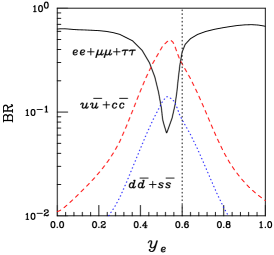
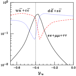
Figure 4: $A_{H}$ Decay branching fractions for $\tan\theta^{\prime}=1$ (a) versus the charged lepton $U(1)$ hypercharge $y_{e}$ with fixed $y_{u}=-0.4$, and (b) versus up-quark hypercharge $y_{u}$ with fixed $y_{e}=0.6$. The vertical dotted lines indicate the hypercharge values determined by the anomaly-free condition.

III.4 New top quark $T$ at the LHC

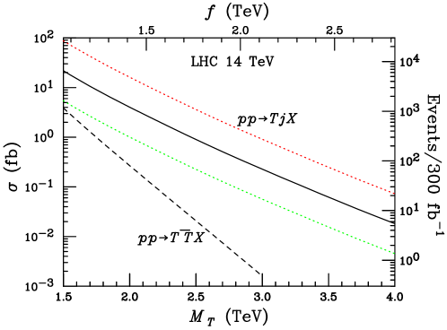
Figure 5: Total cross sections for $T\bar{T}$ production (dashed) and $T+$jet production (solid and dotted) via $t$-channel $W$-exchange versus mass $M_{T}$ at the LHC. The solid line is for the couplings $\lambda_{1}=\lambda_{2}$; the dotted are for $\lambda_{1}/\lambda_{2}=2$ (upper) and 1/2 (lower). The number of events expected per 300 fb^-1 luminosity is indicated on the right-hand axis. The scale $f$ corresponding to $\lambda_{1}=\lambda_{2}$ is given on the top axis.

The new colored vector-like heavy fermion $T$ is also a crucial prediction in little Higgs models. Due to its heavy mass, it may only be produced at high energy hadron colliders. Naively, the leading contribution seems to be from the QCD pair production

$$q\bar{q},\ gg\to T\bar{T}.$$ (49)

However, the phase space suppression of the multi TeV mass becomes rather severe. In contrast, the single $T$ production via $W$-exchange in $t$-channel (or $Wb$ fusion)

$$qb\to q^{\prime}T$$ (50)

falls off much more slowly with the $T$ mass and takes over for $M_{T}$ larger than a few hundred GeV [24]. This is also partially due to the enhanced coupling of the longitudinally polarized gauge bosons at higher energies. In Fig. 5 the cross sections of pair production of $T\bar{T}$ (dashed line) and the single $T$ plus a jet production (solid and dotted) are presented versus its mass $M_{T}$ at the LHC energy. We see that $T+$jet production dominates throughout the mass range of current interest. The solid line is for the choice $\lambda_{1}=\lambda_{2}$, while the dotted are for $\lambda_{1}/\lambda_{2}=2$ and 1/2. We see that for a $T$ with a 3 TeV mass, the cross section can be about 0.23 fb. With an integrated annual luminosity of 300 fb^-1, this corresponds to about 70 events per year, as indicated on the right-hand axis. The other processes of single $T$ production $q\bar{q}^{\prime}\to\bar{b}T$ via $s$-channel $W$-exchange and the associated production $gb\to W_{L}T$ are both much smaller.

Because of the unsuppressed coupling of the heavy top $T$ to the Higgs boson, and the enhanced couplings to the longitudinally polarized gauge bosons (Goldstone bosons), the partial decay widths of $T$ are

$$\Gamma(T\to tH)=\Gamma(T\to tZ)={1\over 2}\Gamma(T\to bW)={\kappa^{2}\over 32\pi}M_{T},$$ (51)

with the coupling $\kappa={\lambda_{1}^{2}/\sqrt{\lambda_{1}^{2}+\lambda_{2}^{2}}}$. Other decay channels are effectively suppressed by $v^{2}/f^{2}$. The total width of $T$ is then given by

$$\Gamma_{T}={\kappa^{2}\over 8\pi}M_{T}={1\over 8\pi}{\lambda_{1}^{2}\over\lambda_{2}^{2}}\left({m_{t}\over v}\right)^{2}M_{T}.$$ (52)

Unlike the SM top quark, whose total width scales as $m_{t}^{3}/v^{2}$, the width of $T$ is linear in $M_{T}$. Regarding the experimental signatures at colliders, all decay channels can be quite identifiable. Although the final state $T\to bW$ takes $50\%$ branching fraction, partly yielding a nice signal of $b$ jet$+\ell^{\pm}$ plus missing energy, the other channels $T\to tH,\ tZ$ may lead to distinctive signatures as well. The $Z$ boson in the final state gives an unambiguous event identification via its leptonic decay, and the system $t(\to bW)Z$ reconstructs $M_{T}$. The Higgs mode can be studied via $t(\to bW)H(\to b\bar{b})$, resulting in three $b$ jets, a charged lepton plus missing energy. Two of the $b$ jets reconstruct $m_{H}$ and the whole transverse mass system reconstructs the large $M_{T}$. There is always a spectator light quark jet ($q^{\prime}$), accompanying $T$, that can be made use of as a forward tagging jet. However, there may be substantial SM backgrounds too, such as $t\bar{t}Z$ to the $T\to tZ$ signal, and $W+4$ QCD jets, $t\bar{t}\to 2b+2$ jets + leptons to the $T\to tH$ signal. More detailed simulations would be needed to make a quantitative conclusion for the $T$ observation.

If a $T$ signal is observed at the LHC, one can deduce the mass scale $f$ based on the relation Eq. (37), leading to $f^{max}=vM_{T}/(2m_{t})\approx{M_{T}/\sqrt{2}},$ which is indicated in Fig. 5 on the top axis. More precise determination can be made when the coupling $\lambda_{1}$ is measured through the production cross section.

III.5 The Higgs sector

The central feature of the model is to have a relatively light neutral Higgs boson $H$. The Higgs mass is typically of the order of $v$. If a Higgs boson is found with a mass greater than 140 GeV, it would imply some new physics different from weak-scale SUSY. However, the deviation of its properties from the minimal SM is rather small in the littlest Higgs model, generically of the order of $v^{2}/f^{2}$, i.e., at a percent level. It would thus be difficult to distinguish this model from the SM even when $H$ has been observed. It has been argued that at a high luminosity $e^{+}e^{-}$ linear collider, the determination of $WWH,\ ZZH$ can be at the $1\%$ level [26]. Inspecting the gauge bosons-Higgs couplings in the littlest Higgs model, we could anticipate a bound

$$f>{v\over\sqrt{3\times 1\%}}\approx 1.4~{}{\rm TeV},$$ (53)

which may not add much new knowledge to our understanding of the model.

Figure 6: Invariant mass distribution of $W^{+}W^{+}$ at the LHC, in the units of the number of events per bin (50 GeV) and per 300 fb^-1. The dashed curve is for $W_{L}^{+}W_{L}^{+}\to W_{L}^{+}W_{L}^{+}$ in the SM and the histograms include the doubly charged Higgs contribution with two representative mass values $M_{\Phi}=1.5,\ 2$ TeV, for $v^{\prime}/v=0.05$.

The would-be Goldstone boson multiplets after the global symmetry breaking are a necessary feature to result in the light Higgs boson, and they generically lead to additional scalar multiplets beyond the SM Higgs doublet. In particular, the doubly charged Higgs state $\Phi^{++}$ from the Higgs triplet may serve as a good signal for this class of models if the coupling is not too small and if it is not too heavy to be accessible at future colliders [27]. We illustrate this point by considering the longitudinal $WW$ scattering

$$W_{L}^{+}W_{L}^{+}\to W_{L}^{+}W_{L}^{+},$$ (54)

which would receive a resonant contribution from $\Phi^{++}\to W^{+}W^{+}$. Figure 6 presents the invariant mass distribution for $M(W^{+}W^{+})$ at the LHC energy. The histograms give the resonant structure for $M_{\Phi}=$ 1.5 and 2 TeV respectively. The dashed curve is the continuum SM $W_{L}^{+}W_{L}^{+}$ background with $M_{H}=120$ GeV. We have used the effective $W$-boson approximation to compute the production rates. In the calculation, we have imposed some cuts on the $W$ transverse momentum and the rapidity as

$$p_{T}>200\ ~{}{\rm GeV},\quad y<3.$$ (55)

The signal cross section is proportional to $v^{\prime 2}/v^{2}$. With the coupling chosen to be $v^{\prime}/v=0.05$ as for Fig. 6, there can be about 120 (30) events near the mass peak of 1.5 (2) TeV for 300 fb^-1 luminosity. Although the like-sign di-leptons may be a spectacular signal for a doubly charged resonance, there are SM backgrounds to be separated. Standard techniques have been developed to identify the $W_{L}^{+}W_{L}^{+}$ signal over the backgrounds [28]. We will not pursue further quantitative evaluation for the signal observability here.

IV Conclusions

The little Higgs models represent a new approach to stabilize the hierarchy between a relatively low cutoff scale $\sim 10$ TeV and the electroweak scale. By linearizing the “littlest Higgs model” [4], we laid out the full structure of the theory to the order of $1/f^{2}$, and discussed its couplings and the mass parameters for the new contents beyond the Standard Model (summarized in Sec. III.1). We explored the symmetry properties in particular related to the custodial $SU(2)$ breaking in the model (Sec. II.3). We also discussed the arbitrariness of the model associated with the $U(1)$ charge assignments for the SM fermions, as well as for the Higgs doublet (Sec. III.2.1).

We have studied the phenomenological consequences of the little Higgs models. The current precision electroweak measurements can put stringent bounds on the model parameters, typically for the scale $f\mathrel{\raise 1.29167pt\hbox{$>$\kern-7.5pt\lower 4.30554pt\hbox{$\sim$}}}3.5-4$ TeV, modulo some arbitrariness of the $U(1)$ charge assignments of the SM particles. By a clever choice of the gauge coupling parameters and fermion hypercharge assignments, the extra contributions to the electroweak precision observables may be significantly suppressed, although even given the freedom of assigning the fermion charges, the particular choice is still a fine-tuning that needs to be justified by a suitable extension of the model. Future precision measurements may further improve the constraints, while reasonable variations of the model associated with the $U(1)$ sector should be kept in mind.

We have also studied the collider phenomenology of the little Higgs model, concentrating on generic signatures that are robust under variation of the details of the model. We found that the LHC has great potential to discover the new $SU(2)$ gauge bosons up to the multi-TeV mass scale. This should serve as the “smoking gun” signature for the little Higgs model, especially if their unique decay branching fractions are measured to a good precision. The possible new $U(1)$ gauge boson may be lighter and be observed earlier at hadron colliders, although its properties are less robust to reflect the little Higgs idea. The colored vector-like quark $T$ is also a unique prediction for little Higgs models, and it may be produced singly through $Wb\to T$ at high energy hadron colliders. It is however typically heavier. The doubly-charged Higgs boson may be the most impressive member of the Higgs sector along with the SM-like Higgs. It can be produced singly via the $W^{+}W^{+}\to\Phi^{++}$ channel and may provide interesting signatures at the LHC. Precision measurements on the triple gauge boson couplings at hadron and especially at future $e^{+}e^{-}$ linear colliders may also shed light on the symmetry breaking scale up to $f\sim 3.5-12$ TeV. Due to the relatively high energy scale of the little Higgs models, multi-TeV lepton colliders would be desirable to explore the new particles and study their properties in detail.

Appendix A The Linearized Lagrangian

We lay out the linearized Lagrangian for the littlest Higgs model in this appendix. The effective non-linear Lagrangian invariant under the local gauge group $G_{1}\otimes G_{2}=[SU(2)_{1}\otimes U(1)_{1}]\otimes[SU(2)_{2}\otimes U(1)_{2}]$ can be written as

$${\mathcal{L}}_{eff}={\mathcal{L}}_{G}+{\mathcal{L}}_{F}+{\mathcal{L}}_{\Sigma}+{\mathcal{L}}_{Y}-V_{CW}(\Sigma),$$ (56)

where $\mathcal{L}_{G}$ consists of the pure gauge terms; $\mathcal{L}_{F}$ the fermion kinetic terms; $\mathcal{L}_{\Sigma}$ the $\sigma$-Model terms of the littlest Higgs model; $\mathcal{L}_{Y}$ the Yukawa couplings of fermions and pseudo-Goldstone bosons; and $V_{CW}(\Sigma)$ the Coleman-Weinberg potential, generated radiatively from $\mathcal{L}_{\Sigma},\ \mathcal{L}_{Y}$. We now discuss each individual term in detail. In order to obtain the effective Lagrangian in terms of the physical fields, we need to expand the nonlinear $\sigma$-model in a consistent fashion, which corresponds to expansion in $1/f$.

A.1 $\mathcal{L}_{\Sigma}$: Scalar kinetic terms and the heavy gauge bosons

At the scale $\Lambda_{S}\sim 4\pi f$, the vev associated with the spontaneous symmetry breaking proportional to the scale $f$ is parameterized by the $5\times 5$ symmetrical matrix [4]

$$\Sigma_{0}=\left(\begin{array}[]{ccc}&&{\mathbf{1}}_{2\times 2}\\ &1&\\ {\mathbf{1}}_{2\times 2}&&\end{array}\right).$$ (57)

Turning on this vev breaks the assumed global $SU(5)$ symmetry into its subgroup $SO(5)$. The appearance of the condensate also breaks the assumed local gauge symmetry $[SU(2)\otimes U(1)]^{2}$ into its diagonal subgroup $[SU(2)\otimes U(1)]_{SM}$. The scalar fields are parameterized by

$$\Sigma=e^{i\Pi/f}\ \Sigma_{0}\ e^{i\Pi^{T}/f},$$ (58)

that transforms under the gauge group as

$$\Sigma\to\Sigma^{\prime}=U\ \Sigma\ U^{T},$$ (59)

where $U=L_{1}Y_{1}L_{2}Y_{2}$ is an element of the gauge groups. Here $f$ is the Goldstone boson decay constant, and the Goldstone boson matrix $\Pi$ is expressed by

$$\Pi=\left(\begin{array}[]{ccc}{}\hfil&h^{\dagger}/\sqrt{2}&\phi^{\dagger}\\ h/\sqrt{2}&{}\hfil&h^{*}/\sqrt{2}\\ \phi&h^{T}/\sqrt{2}&{}\hfil\end{array}\right),$$ (60)

where the scalar field content consists of a doublet $h$ and a triplet $\phi$ under the unbroken $SU(2)_{L}\otimes U(1)_{Y}$ SM gauge group

$$h=(h^{+},h^{0}),\qquad\phi=\left(\begin{array}[]{cc}\phi^{++}&\frac{\phi^{+}}{\sqrt{2}}\\ \frac{\phi^{+}}{\sqrt{2}}&\phi^{0}\end{array}\right).$$ (61)

For phenomenological studies, it is important to linearize the effective Lagrangian and write it in terms of the couplings of gauge bosons and $h$, $\phi$. This can be achieved by expanding $\Sigma$ around its vacuum expectation value in powers of ${1}/{f}$

$$\Sigma=\Sigma_{0}+\frac{2i}{f}\left(\begin{array}[]{ccccc}\phi^{\dagger}&\frac{h^{\dagger}}{\sqrt{2}}&{\mathbf{0}}_{2\times 2}\\ \frac{h^{*}}{\sqrt{2}}&0&\frac{h}{\sqrt{2}}\\ {\mathbf{0}}_{2\times 2}&\frac{h^{T}}{\sqrt{2}}&\phi\end{array}\right)-\frac{1}{f^{2}}\left(\begin{array}[]{ccc}h^{\dagger}h^{*}&\sqrt{2}\phi^{\dagger}h^{T}&h^{\dagger}h+2\phi^{\dagger}\phi\\ \sqrt{2}h\phi^{\dagger}&2hh^{\dagger}&\sqrt{2}h^{*}\phi\\ h^{T}h^{*}+2\phi\phi^{\dagger}&\sqrt{2}\phi h^{\dagger}&h^{T}h\end{array}\right)+{\cal O}(\frac{1}{f^{3}}).$$ (62)

The leading order dimension-two term in the non-linear $\sigma$-model can be written for the scalar sector as

$$\mathcal{L}_{\Sigma}=\frac{1}{2}\frac{f^{2}}{4}{\rm Tr}|\mathcal{D}_{\mu}\Sigma|^{2}.$$ (63)

The numerical coefficients have been chosen so that the scalar kinetic terms are canonically normalized. It is manifestly gauge invariant under $G_{1}\otimes G_{2}=[SU(2)_{1}\otimes U(1)_{1}]\otimes[SU(2)_{2}\otimes U(1)_{2}]$ if the covariant derivative is defined as

$$\mathcal{D}_{\mu}\Sigma=\partial_{\mu}\Sigma-i\sum_{j=1}^{2}\left(g_{j}(W_{j}\Sigma+\Sigma W_{j}^{T})+g^{\prime}_{j}(B_{j}\Sigma+\Sigma B_{j}^{T})\right),$$ (64)

where the $SU(2)$ gauge fields are $W_{j}=\sum_{a=1}^{3}W_{\mu j}^{a}Q_{j}^{a}$ with

$$Q_{1}^{a}=\left(\begin{array}[]{ccc}\frac{\sigma^{a}}{2}&&\\ &&\\ &&{\mathbf{0}}_{3\times 3}\end{array}\right),\qquad Q_{2}^{a}=\left(\begin{array}[]{ccc}{\mathbf{0}}_{3\times 3}&&\\ &&\\ &&-\frac{\sigma^{a*}}{2}\end{array}\right).$$ (65)

Similarly, the $U(1)$ gauge fields are $B_{j}=B_{\mu j}Y_{j}$ with

$$Y_{1}=\frac{1}{10}\left(\begin{array}[]{ccccc}-3&&&&\\ &-3&&&\\ &&2&&\\ &&&2&\\ &&&&2\end{array}\right),\qquad Y_{2}=\frac{1}{10}\left(\begin{array}[]{ccccc}-2&&&&\\ &-2&&&\\ &&-2&&\\ &&&3&\\ &&&&3\end{array}\right).$$ (66)

The vacuum expectation value (vev) of the $\Sigma$ field breaks the $[SU(2)\otimes U(1)]_{1}\otimes[SU(2)\otimes U(1)]_{2}$ gauge symmetry down to the diagonal subgroup, with the broken generators (associated with $W^{\prime}$)

$$Q^{\prime a}=\frac{1}{\sqrt{g_{1}^{4}+g_{2}^{4}}}(g_{1}^{2}Q_{1}^{a}-g_{2}^{2}Q_{2}^{a}).$$ (67)

and the unbroken $SU(2)_{L}\otimes U(1)_{Y}$ gauge generators

$$Q^{a}=\frac{1}{\sqrt{2}}(Q_{1}^{a}+Q_{2}^{a}),\qquad Y=Y_{1}+Y_{2}.$$ (68)

The spontaneous gauge symmetry breaking thereby gives rise to mass terms of order $f$ for the gauge bosons

$$\mathcal{L}_{\Sigma}(mass) = \frac{1}{2}\frac{f^{2}}{4}\left[g_{1}^{2}W_{1\mu}^{a}W_{1}^{a\mu}+g_{2}^{2}W_{2\mu}^{a}W_{2}^{a\mu}-2g_{1}g_{2}W_{1\mu}^{a}W_{2}^{a\mu}\right]$$ (69)

$$+ \frac{1}{2}\frac{f^{2}}{4}\frac{1}{5}\left[g_{1}^{\prime 2}B_{1\mu}B_{1}^{\mu}+g_{2}^{\prime 2}B_{2\mu}B_{2}^{\mu}-2g_{1}^{\prime}g_{2}^{\prime}B_{1\mu}B_{2}^{\mu}\right].$$

We define

$$W=sW_{1}+cW_{2}, W^{\prime}=-cW_{1}+sW_{2}$$

$$B=s^{\prime}B_{1}+c^{\prime}B_{2}, B^{\prime}=-c^{\prime}B_{1}+s^{\prime}B_{2},$$ (70)

where the mixing angles are given by:

$$s=\frac{g_{2}}{\sqrt{g_{1}^{2}+g_{2}^{2}}}, c=\frac{g_{1}}{\sqrt{g_{1}^{2}+g_{2}^{2}}}$$

$$s^{\prime}=\frac{g_{2}^{\prime}}{\sqrt{g_{1}^{\prime 2}+g_{2}^{\prime 2}}}, c^{\prime}=\frac{g_{1}^{\prime}}{\sqrt{g_{1}^{\prime 2}+g_{2}^{\prime 2}}}.$$ (71)

The heavy gauge boson masses are then

$$m_{W^{\prime}}=\frac{f}{2}\sqrt{g_{1}^{2}+g_{2}^{2}}=\frac{g}{2sc}f,\qquad m_{B^{\prime}}=\frac{f}{2\sqrt{5}}\sqrt{g_{1}^{\prime 2}+g_{2}^{\prime 2}}=\frac{g^{\prime}}{2\sqrt{5}s^{\prime}c^{\prime}}f.$$ (72)

The massless states $W$ and $B$ are identified as the SM gauge bosons, with couplings

$$g=g_{1}s=g_{2}c,\qquad g^{\prime}=g_{1}^{\prime}s^{\prime}=g_{2}^{\prime}c^{\prime}.$$ (73)

A.2 $V_{CW}$: Effective Higgs potential and the electroweak symmetry breaking

In the littlest Higgs model, the global symmetries prevent the appearance of a Higgs potential at tree level. Instead, the Higgs potential is generated at one-loop and higher orders due to interactions with the gauge bosons and fermions. The quadratically divergent contributions to this Coleman-Weinberg potential are cut off by the scale $\Lambda_{S}$. In practice, these are proportional to $\Lambda_{S}^{2}/16\pi^{2}\sim f^{2}$. The unknown ultraviolet physics at the cutoff scale $\Lambda_{S}$ is parameterized by $\mathcal{O}(1)$ coefficients $a$ and $a^{\prime}$.

The most important terms of the Coleman-Weinberg potential can be parameterized as:

$$V=\lambda_{\phi^{2}}f^{2}{\rm Tr}(\phi^{\dagger}\phi)+i\lambda_{h\phi h}f\left(h\phi^{\dagger}h^{T}-h^{*}\phi h^{\dagger}\right)-\mu^{2}hh^{\dagger}+\lambda_{h^{4}}(hh^{\dagger})^{2},$$ (74)

where we neglect quartic terms involving $\phi^{4}$ and $h^{2}\phi^{2}$ since they give only sub-leading contributions to the vacuum expectation values and the scalar field masses.

The quadratically divergent contribution to the Coleman-Weinberg potential from vector boson loops is [4]

$$\mathcal{L}_{a}=\frac{1}{2}af^{4}\left\{g_{j}^{2}\sum_{a}{\rm Tr}\left[\left(Q_{j}^{a}\Sigma\right)\left(Q_{j}^{a}\Sigma\right)^{*}\right]+g_{j}^{\prime 2}{\rm Tr}\left[\left(Y_{j}\Sigma\right)\left(Y_{j}\Sigma\right)^{*}\right]\right\}.$$ (75)

Linearizing the $\Sigma$ field, we obtain

$$\mathcal{L}_{a} = \frac{a}{2}(g_{1}^{2}+g_{1}^{\prime 2})\left[f^{2}{\rm Tr}\left(\phi^{\dagger}\phi\right)-\frac{if}{2}\left(h\phi^{\dagger}h^{T}-h^{*}\phi h^{\dagger}\right)+\frac{1}{4}\left(hh^{\dagger}\right)^{2}+\cdots\right]$$ (76)

$$+ \frac{a}{2}(g_{2}^{2}+g_{2}^{\prime 2})\left[f^{2}{\rm Tr}\left(\phi^{\dagger}\phi\right)+\frac{if}{2}\left(h\phi^{\dagger}h^{T}-h^{*}\phi h^{\dagger}\right)+\frac{1}{4}\left(hh^{\dagger}\right)^{2}+\cdots\right].$$

The $[SU(2)\otimes U(1)]_{1}$ interactions preserve the $SU(3)_{2}$ global symmetry in the lower $3\times 3$ block of $\Sigma$, while the $[SU(2)\otimes U(1)]_{2}$ interactions preserve the $SU(3)_{1}$ global symmetry in the upper $3\times 3$ block of $\Sigma$.

The quadratically divergent contribution to the Coleman-Weinberg potential from fermion loops is [4]

$$\mathcal{L}_{a^{\prime}} = -a^{\prime}\frac{1}{4}\lambda_{1}^{2}f^{4}\epsilon^{wx}\epsilon_{yz}\epsilon^{ijk}\epsilon_{kmn}\Sigma_{iw}\Sigma_{jx}\Sigma^{*my}\Sigma^{*nz},$$ (77)

where $i,j,k,m,n$ run over $1,2,3$ and $w,x,y,z$ run over $4,5$. To fourth order in $h$ and second order in $\phi$, this term leads to

$$\mathcal{L}_{a^{\prime}} = 8a^{\prime}\lambda_{1}^{2}\left[f^{2}{\rm Tr}\left(\phi^{\dagger}\phi\right)+\frac{if}{2}\left(h\phi^{\dagger}h^{T}-h^{*}\phi h^{\dagger}\right)+\frac{1}{4}\left(hh^{\dagger}\right)^{2}+\cdots\right].$$ (78)

The fermion interactions that give rise to this term preserve the $SU(3)_{1}$ global symmetry in the upper $3\times 3$ block of $\Sigma$, so this contribution to the potential must have the same form as the term proportional to $(g_{2}^{2}+g_{2}^{\prime 2})$ in Eq. (76).

The coefficients $\lambda_{\phi^{2}}$, $\lambda_{h\phi h}$ and $\lambda_{h^{4}}$ in Eq. (74) are therefore given by:

$$\lambda_{\phi^{2}} = \frac{a}{2}\left[\frac{g^{2}}{s^{2}c^{2}}+\frac{g^{\prime 2}}{s^{\prime 2}c^{\prime 2}}\right]+8a^{\prime}\lambda_{1}^{2},$$

$$\lambda_{h\phi h} = -\frac{a}{4}\left[g^{2}\frac{(c^{2}-s^{2})}{s^{2}c^{2}}+g^{\prime 2}\frac{(c^{\prime 2}-s^{\prime 2})}{s^{\prime 2}c^{\prime 2}}\right]+4a^{\prime}\lambda_{1}^{2},$$

$$\lambda_{h^{4}} = \frac{a}{8}\left[\frac{g^{2}}{s^{2}c^{2}}+\frac{g^{\prime 2}}{s^{\prime 2}c^{\prime 2}}\right]+2a^{\prime}\lambda_{1}^{2}=\frac{1}{4}\lambda_{\phi^{2}}.$$ (79)

Here we have neglected the log-divergent one-loop and quadratically divergent two-loop contributions to the effective couplings in Eq. (79). These are suppressed by a loop factor $1/16\pi^{2}$ compared to the leading terms given here.

The coefficient $\mu^{2}$ of the $hh^{\dagger}$ term is a free parameter since this term gets equally significant contributions from the one-loop log-divergent and two-loop quadratically-divergent parts of the Coleman-Weinberg potential. At one-loop order, $\mu^{2}$ gets a contribution from the log-divergent terms of order $f^{2}\log(\Lambda_{S}^{2}/f^{2})/(16\pi^{2})$, giving a natural hierarchy between the TeV scale $f$ and the electroweak scale. At two-loop order, $\mu^{2}$ gets a contribution from the quadratically-divergent term of order $\Lambda_{S}^{2}/(16\pi^{2})^{2}\sim f^{2}/16\pi^{2}$, with an arbitrary coefficient of order unity determined by the UV completion. We thus write the coefficient as a new free parameter $\mu^{2}\sim f^{2}/16\pi^{2}$.

For $\mu^{2}>0$, this scalar potential triggers electroweak symmetry breaking, resulting in the vacuum expectation values for the $h$ and $\phi$ fields: $\langle h^{0}\rangle=v/\sqrt{2}$ and $\langle i\phi^{0}\rangle=v^{\prime}$, with

$$v^{2}=\frac{\mu^{2}}{\lambda_{h^{4}}-\lambda_{h\phi h}^{2}/\lambda_{\phi^{2}}},\qquad v^{\prime}=\frac{\lambda_{h\phi h}}{2\lambda_{\phi^{2}}}\frac{v^{2}}{f}.$$ (80)

The gauge eigenstates of the Higgs fields $h$ and $\phi$ can be written in terms of the mass eigenstates as follows:

$$h^{0} = \left(c_{0}H-s_{0}\Phi^{0}+v\right)/\sqrt{2}+i\left(c_{P}G^{0}-s_{P}\Phi^{P}\right)/\sqrt{2},$$

$$\phi^{0} = \left(s_{P}G^{0}+c_{P}\Phi^{P}\right)/\sqrt{2}-i\left(s_{0}H+c_{0}\Phi^{0}+\sqrt{2}v^{\prime}\right)/\sqrt{2},$$

$$h^{+} = c_{+}G^{+}-s_{+}\Phi^{+},\qquad\phi^{+}=\left(s_{+}G^{+}+c_{+}\Phi^{+}\right)/i$$

$$\phi^{++} = \Phi^{++}/i.$$ (81)

We use the following notation for the physical mass eigenstates: $H$ and $\Phi^{0}$ are neutral scalars, $\Phi^{P}$ is a neutral pseudoscalar, $\Phi^{+}$ and $\Phi^{++}$ are the charged and doubly charged scalars, and $G^{+}$ and $G^{0}$ are the Goldstone bosons that are eaten by the light $W$ and $Z$ bosons, giving them mass. Note that in defining the mass eigenstates we have factored out an $i$ from $\phi$.

The mixing angles in the pseudoscalar and singly-charged sectors are easily extracted in terms of the vacuum expectation values:

$$s_{P} = \frac{2\sqrt{2}v^{\prime}}{\sqrt{v^{2}+8v^{\prime 2}}}\simeq 2\sqrt{2}\frac{v^{\prime}}{v},\qquad c_{P}=\frac{v}{\sqrt{v^{2}+8v^{\prime 2}}}\simeq 1-4\frac{v^{\prime 2}}{v^{2}}$$

$$s_{+} = \frac{2v^{\prime}}{\sqrt{v^{2}+4v^{\prime 2}}}\simeq 2\frac{v^{\prime}}{v},\qquad c_{+}=\frac{v}{\sqrt{v^{2}+4v^{\prime 2}}}\simeq 1-2\frac{v^{\prime 2}}{v^{2}}.$$ (82)

Diagonalizing the mass terms for the neutral CP-even scalars gives the scalar mixing angle $s_{0},c_{0}$ to leading order in $v/f$:

$$s_{0}\simeq 2\sqrt{2}\frac{v^{\prime}}{v},\qquad c_{0}\simeq 1-4\frac{v^{\prime 2}}{v^{2}}.$$ (83)

Note that to leading order $s_{0}=s_{P}=\sqrt{2}s_{+}\sim\mathcal{O}(v/f)$.

To leading order, all of the triplet $\Phi$ states are degenerate in mass. The masses of $\Phi$ and $H$ are

$$M^{2}_{\Phi}\simeq\lambda_{\phi^{2}}f^{2},\qquad m^{2}_{H}\simeq 2\left(\lambda_{h^{4}}-\lambda_{h\phi h}^{2}/\lambda_{\phi^{2}}\right)v^{2}=2\mu^{2}.$$ (84)

A.3 Gauge boson masses and mixing from $\mathcal{L}_{\Sigma}$

After EWSB, the gauge sector gets additional mass and mixing terms due to the $h$ and $\phi$ vevs. The full set of mass terms after EWSB is:

$$\mathcal{L}_{\Sigma}(masses) = \frac{1}{2}W_{\mu}^{\prime a}W^{\prime a\mu}\left[m_{W^{\prime}}^{2}-\frac{1}{4}g^{2}v^{2}\right]+W_{\mu}^{+}W^{-\mu}\left[\frac{1}{4}g^{2}v^{2}\left(1-\frac{v^{2}}{6f^{2}}+4\frac{v^{\prime 2}}{v^{2}}\right)\right]$$ (85)

$$+\frac{1}{2}W_{\mu}^{3}W^{3\mu}\left[\frac{1}{4}g^{2}v^{2}\left(1-\frac{v^{2}}{6f^{2}}+8\frac{v^{\prime 2}}{v^{2}}\right)\right]$$

$$-W_{\mu}^{a}W^{\prime a\mu}\left[\frac{1}{4}g^{2}v^{2}\frac{(c^{2}-s^{2})}{2sc}\right]+\frac{1}{2}B_{\mu}^{\prime}B^{\prime\mu}\left[m_{B^{\prime}}^{2}-\frac{1}{4}g^{\prime 2}v^{2}\right]$$

$$+\frac{1}{2}B_{\mu}B^{\mu}\left[\frac{1}{4}g^{\prime 2}v^{2}\left(1-\frac{v^{2}}{6f^{2}}+8\frac{v^{\prime 2}}{v^{2}}\right)\right]-B_{\mu}B^{\prime\mu}\left[\frac{1}{4}g^{\prime 2}v^{2}\frac{(c^{\prime 2}-s^{\prime 2})}{2s^{\prime}c^{\prime}}\right]$$

$$+W_{\mu}^{3}B^{\mu}\left[\frac{1}{4}gg^{\prime}v^{2}\left(1-\frac{v^{2}}{6f^{2}}+8\frac{v^{\prime 2}}{v^{2}}\right)\right]+W_{\mu}^{\prime 3}B^{\prime\mu}\left[-\frac{1}{8}gg^{\prime}v^{2}\left(\frac{cs^{\prime}}{sc^{\prime}}+\frac{sc^{\prime}}{cs^{\prime}}\right)\right]$$

$$-W_{\mu}^{3}B^{\prime\mu}\left[\frac{1}{4}gg^{\prime}v^{2}\frac{(c^{\prime 2}-s^{\prime 2})}{2s^{\prime}c^{\prime}}\right]-W_{\mu}^{\prime 3}B^{\mu}\left[\frac{1}{4}gg^{\prime}v^{2}\frac{(c^{2}-s^{2})}{2sc}\right],$$

where for the $WW$, $BB$ and $WB$ terms we have included terms up to order $v^{4}/f^{2}$; these will be necessary in order to find the masses of the light gauge bosons consistently to this order.

A.3.1 Charged gauge bosons

Let us first consider the charged $W,W^{\prime}$ sector. The charged $W,W^{\prime}$ mass eigenstates, to order $v^{2}/f^{2}$, are:

$$W_{L}=W+\frac{v^{2}}{2f^{2}}sc(c^{2}-s^{2})W^{\prime},\qquad W_{H}=W^{\prime}-\frac{v^{2}}{2f^{2}}sc(c^{2}-s^{2})W.$$ (86)

The masses of $W_{L}$ (light) and $W_{H}$ (heavy) to the order of $v^{2}/f^{2}$ are given by:

$$M_{W_{L}^{\pm}}^{2} = m_{w}^{2}\left[1-\frac{v^{2}}{f^{2}}\left(\frac{1}{6}+\frac{1}{4}(c^{2}-s^{2})^{2}\right)+4\frac{v^{\prime 2}}{v^{2}}\right],$$ (87)

$$M_{W_{H}^{\pm}}^{2} = \frac{f^{2}g^{2}}{4s^{2}c^{2}}-\frac{1}{4}g^{2}v^{2}+\mathcal{O}(v^{4}/f^{2})=m_{w}^{2}\left(\frac{f^{2}}{s^{2}c^{2}v^{2}}-1\right),$$ (88)

where $m_{w}\equiv gv/2$.

A.3.2 Neutral gauge bosons

The four neutral gauge boson mass eigenstates to the order $v^{2}/f^{2}$ are:

$$A_{L} = s_{{\rm w}}W^{3}+c_{{\rm w}}B$$

$$Z_{L} = c_{{\rm w}}W^{3}-s_{{\rm w}}B+x_{Z}^{W^{\prime}}\frac{v^{2}}{f^{2}}W^{\prime 3}+x_{Z}^{B^{\prime}}\frac{v^{2}}{f^{2}}B^{\prime}$$

$$A_{H} = B^{\prime}+x_{H}\frac{v^{2}}{f^{2}}W^{\prime 3}-x_{Z}^{B^{\prime}}\frac{v^{2}}{f^{2}}(c_{{\rm w}}W^{3}-s_{{\rm w}}B)$$

$$Z_{H} = W^{\prime 3}-x_{H}\frac{v^{2}}{f^{2}}B^{\prime}-x_{Z}^{W^{\prime}}\frac{v^{2}}{f^{2}}(c_{{\rm w}}W^{3}-s_{{\rm w}}B),$$ (89)

where

$$x_{H} = \frac{5}{2}gg^{\prime}\frac{scs^{\prime}c^{\prime}(c^{2}s^{\prime 2}+s^{2}c^{\prime 2})}{(5g^{2}s^{\prime 2}c^{\prime 2}-g^{\prime 2}s^{2}c^{2})},$$

$$x_{Z}^{W^{\prime}} = -\frac{1}{2c_{{\rm w}}}sc(c^{2}-s^{2}),\qquad x_{Z}^{B^{\prime}}=-\frac{5}{2s_{{\rm w}}}s^{\prime}c^{\prime}(c^{\prime 2}-s^{\prime 2}).$$ (90)

The weak mixing angle is defined as usual:

$$s_{{\rm w}}=\frac{g^{\prime}}{\sqrt{g^{2}+g^{\prime 2}}}, c_{{\rm w}}=\frac{g}{\sqrt{g^{2}+g^{\prime 2}}}.$$ (91)

The neutral gauge boson masses are:

$$M_{A_{L}}^{2} = 0$$

$$M_{Z_{L}}^{2} = m_{z}^{2}\left[1-\frac{v^{2}}{f^{2}}\left(\frac{1}{6}+\frac{1}{4}(c^{2}-s^{2})^{2}+\frac{5}{4}(c^{\prime 2}-s^{\prime 2})^{2}\right)+8\frac{v^{\prime 2}}{v^{2}}\right]$$

$$M_{A_{H}}^{2} = \frac{f^{2}g^{\prime 2}}{20s^{\prime 2}c^{\prime 2}}-\frac{1}{4}g^{\prime 2}v^{2}+g^{2}v^{2}\frac{x_{H}}{4s^{2}c^{2}}=m_{z}^{2}s_{{\rm w}}^{2}\left(\frac{f^{2}}{5s^{\prime 2}c^{\prime 2}v^{2}}-1+\frac{x_{H}c_{{\rm w}}^{2}}{4s^{2}c^{2}s_{{\rm w}}^{2}}\right)$$

$$M_{Z_{H}}^{2} = \frac{f^{2}g^{2}}{4s^{2}c^{2}}-\frac{1}{4}g^{2}v^{2}-g^{\prime 2}v^{2}\frac{x_{H}}{4s^{\prime 2}c^{\prime 2}}=m_{w}^{2}\left(\frac{f^{2}}{s^{2}c^{2}v^{2}}-1-\frac{x_{H}s_{{\rm w}}^{2}}{s^{\prime 2}c^{\prime 2}c_{{\rm w}}^{2}}\right),$$ (92)

where $m_{z}\equiv{gv}/(2c_{{\rm w}})$. Again, note that the $Z_{L}$ mass gets a correction at order $v^{2}/f^{2}$.

A.4 Scalar-fermion couplings: The Yukawa interactions $\mathcal{L}_{Y}$

The scalar couplings to the top quark can be taken as [4]

$${\mathcal{L}}_{Y}=\frac{1}{2}\lambda_{1}f\epsilon_{ijk}\epsilon_{xy}\chi_{i}\Sigma_{jx}\Sigma_{ky}u^{\prime c}_{3}+\lambda_{2}f\tilde{t}\tilde{t}^{\prime c}+{\rm h.c.},$$ (93)

where $\chi_{i}=(b_{3},t_{3},\tilde{t})$. The factor of $1/2$ normalization in front of $\lambda_{1}$ makes our notation simpler. Expanding the $\Sigma$ field generates the scalar interactions with quarks:

$$\mathcal{L}_{t} = \lambda_{2}f\tilde{t}\tilde{t}^{\prime c}+i\lambda_{1}\left\{-b_{3}\left[\sqrt{2}h^{+}+\frac{i}{f}(\sqrt{2}h^{-}\phi^{++}+h^{0*}\phi^{+})\right]u_{3}^{\prime c}\right.$$

$$\qquad-t_{3}\left[\sqrt{2}h^{0}+\frac{i}{f}(h^{-}\phi^{+}+\sqrt{2}h^{0*}\phi^{0})\right]u_{3}^{\prime c}$$

$$\qquad\left.+\tilde{t}\left[-if+\frac{i}{f}(h^{+}h^{-}+h^{0}h^{0*}+2\phi^{++}\phi^{--}+2\phi^{+}\phi^{-}+2\phi^{0}\phi^{0*})\right]u_{3}^{\prime c}\right\}+{\rm h.c.}$$

This Lagrangian contains a mass term of order $f$ that couples $\tilde{t}$ to a linear combination of $\tilde{t}^{\prime c}$ and $u_{3}^{\prime c}$. Defining mixtures of $\tilde{t}^{c}$ and $u_{3}^{\prime c}$ as follows,

$$\tilde{t}^{c} = \frac{1}{\sqrt{\lambda_{1}^{2}+\lambda_{2}^{2}}}(\lambda_{2}\tilde{t}^{\prime c}+\lambda_{1}u_{3}^{\prime c}),\qquad u_{3}^{c}=\frac{1}{\sqrt{\lambda_{1}^{2}+\lambda_{2}^{2}}}(-\lambda_{1}\tilde{t}^{\prime c}+\lambda_{2}u_{3}^{\prime c}),$$ (95)

diagonalizes the mass term for the heavy fermions:

$$\mathcal{L}_{f}=f\sqrt{\lambda_{1}^{2}+\lambda_{2}^{2}}\tilde{t}\tilde{t}^{c}=-m_{\tilde{t}}\tilde{t}\tilde{t}^{c}.$$ (96)

The rest of the Lagrangian reads:

$$\mathcal{L}_{f} = -\frac{\sqrt{2}i\lambda_{1}^{2}}{\sqrt{\lambda_{1}^{2}+\lambda_{2}^{2}}}\left[b_{3}h^{+}\tilde{t}^{c}+t_{3}h^{0}\tilde{t}^{c}\right]-\frac{\sqrt{2}i\lambda_{1}\lambda_{2}}{\sqrt{\lambda_{1}^{2}+\lambda_{2}^{2}}}\left[b_{3}h^{+}u_{3}^{c}+t_{3}h^{0}u_{3}^{c}\right]$$ (97)

$$+\frac{\lambda_{1}^{2}}{\sqrt{\lambda_{1}^{2}+\lambda_{2}^{2}}}\frac{1}{f}\left[b_{3}(\sqrt{2}h^{-}\phi^{++}+h^{0*}\phi^{+})\tilde{t}^{c}+t_{3}(h^{-}\phi^{+}+\sqrt{2}h^{0*}\phi^{0})\tilde{t}^{c}\right.$$

$$\left.-\tilde{t}(h^{+}h^{-}+h^{0}h^{0*}+2\phi^{++}\phi^{--}+2\phi^{+}\phi^{-}+2\phi^{0}\phi^{0*})\tilde{t}^{c}\right]$$

$$+\frac{\lambda_{1}\lambda_{2}}{\sqrt{\lambda_{1}^{2}+\lambda_{2}^{2}}}\frac{1}{f}\left[b_{3}(\sqrt{2}h^{-}\phi^{++}+h^{0*}\phi^{+})u_{3}^{c}+t_{3}(h^{-}\phi^{+}+\sqrt{2}h^{0*}\phi^{0})u_{3}^{c}\right.$$

$$\left.-\tilde{t}(h^{+}h^{-}+h^{0}h^{0*}+2\phi^{++}\phi^{--}+2\phi^{+}\phi^{-}+2\phi^{0}\phi^{0*})u_{3}^{c}\right]+\mathcal{O}(1/f^{2})+{\rm h.c.}$$

Electroweak symmetry breaking generates additional mass terms for the fermions:

$$\mathcal{L}_{f} = \left[f\sqrt{\lambda_{1}^{2}+\lambda_{2}^{2}}-\frac{\lambda_{1}^{2}}{\sqrt{\lambda_{1}^{2}+\lambda_{2}^{2}}}\frac{v^{2}}{2f}\right]\tilde{t}\tilde{t}^{c}-\frac{i\lambda_{1}^{2}v}{\sqrt{\lambda_{1}^{2}+\lambda_{2}^{2}}}\left[1+\frac{v^{2}}{f^{2}}\left(-\frac{1}{3}+\frac{fv^{\prime}}{v^{2}}\right)\right]t_{3}\tilde{t}^{c}$$ (98)

$$-\frac{\lambda_{1}\lambda_{2}}{\sqrt{\lambda_{1}^{2}+\lambda_{2}^{2}}}\frac{v^{2}}{2f}\tilde{t}u_{3}^{c}-\frac{i\lambda_{1}\lambda_{2}v}{\sqrt{\lambda_{1}^{2}+\lambda_{2}^{2}}}\left[1+\frac{v^{2}}{f^{2}}\left(-\frac{1}{3}+\frac{fv^{\prime}}{v^{2}}\right)\right]t_{3}u_{3}^{c}.$$

The factor of $i$ in the $t_{3}u_{3}^{c}$ and $t_{3}\tilde{t}^{c}$ mass terms can be absorbed into a re-phasing of the left-handed quark doublet field; instead we keep it explicitly for simplicity.

After diagonalizing these mass terms, we obtain the physical top quark $t$ and a new heavy quark $T$:

$$t_{L}=c_{L}t_{3}-s_{L}\tilde{t}, t_{R}^{c}=c_{R}u_{3}^{\prime c}-s_{R}\tilde{t}^{\prime c},$$

$$T_{L}=s_{L}t_{3}+c_{L}\tilde{t}, T_{R}^{c}=s_{R}u_{3}^{\tilde{c}}+c_{R}\tilde{t}^{\prime c},$$

where

$$s_{R} = \frac{\lambda_{1}}{\sqrt{\lambda_{1}^{2}+\lambda_{2}^{2}}}\left[1-\frac{v^{2}}{f^{2}}\frac{\lambda_{2}^{2}}{\lambda_{1}^{2}+\lambda_{2}^{2}}\left(\frac{1}{2}+\frac{\lambda_{1}^{2}}{\lambda_{1}^{2}+\lambda_{2}^{2}}\right)\right],$$

$$c_{R} = \frac{\lambda_{2}}{\sqrt{\lambda_{1}^{2}+\lambda_{2}^{2}}}\left[1+\frac{v^{2}}{f^{2}}\frac{\lambda_{1}^{2}}{\lambda_{1}^{2}+\lambda_{2}^{2}}\left(\frac{1}{2}+\frac{\lambda_{1}^{2}}{\lambda_{1}^{2}+\lambda_{2}^{2}}\right)\right],$$

$$s_{L} = -i\frac{\lambda_{1}^{2}}{\lambda_{1}^{2}+\lambda_{2}^{2}}\frac{v}{f}\left[1-\frac{v^{2}}{f^{2}}\left(\frac{5}{6}-\frac{fv^{\prime}}{v^{2}}-\frac{1}{2}\frac{\lambda_{1}^{4}}{(\lambda_{1}^{2}+\lambda_{2}^{2})^{2}}\right)\right],$$

$$c_{L} = 1-\frac{v^{2}}{2f^{2}}\frac{\lambda_{1}^{4}}{(\lambda_{1}^{2}+\lambda_{2}^{2})^{2}}.$$ (99)

The corresponding masses are:

$$m_{t} = \frac{i\lambda_{1}\lambda_{2}}{\sqrt{\lambda_{1}^{2}+\lambda_{2}^{2}}}v\left\{1+\frac{v^{2}}{f^{2}}\left[-\frac{1}{3}+\frac{fv^{\prime}}{v^{2}}+\frac{1}{2}\frac{\lambda_{1}^{2}}{\lambda_{1}^{2}+\lambda_{2}^{2}}\left(1-\frac{\lambda_{1}^{2}}{\lambda_{1}^{2}+\lambda_{2}^{2}}\right)\right]\right\},$$

$$M_{T} = -f\sqrt{\lambda_{1}^{2}+\lambda_{2}^{2}}\left[1+\mathcal{O}(v^{2}/f^{2})\right].$$ (100)

The scalar interactions with the up-type quarks of the first two generations take the same form as in Eq. (93), except that there is no need for the extra vector-like quarks $\tilde{t},\tilde{t}^{\prime c}$. The interactions with the down-type quarks $d^{c}$ and leptons of the three generations are generated by a similar Lagrangian, again without the extra quarks, and can be written as

$${\mathcal{L}}_{Y}=\frac{1}{2}\lambda_{d}f\epsilon_{ijk}\epsilon_{xy}\chi_{i}\Sigma_{jx}^{*}\Sigma_{ky}^{*}d^{c}+{\rm h.c.}$$ (101)

with the isospin index $i=1,2$ only, and similarly for the leptons.

A.5 Fermion kinetic terms $\mathcal{L}_{F}$

The fermion gauge interactions take the generic form

$$\mathcal{L}_{F} = \sum_{f}\overline{\psi}_{f}i\gamma^{\mu}D_{\mu}\psi_{f},\quad f={\rm flavor\ and\ chirality}$$ (102)

$$D_{\mu} = \partial_{\mu}-i\sum_{j=1}^{2}(g_{j}W_{j\mu}+g^{\prime}_{j}B_{j\mu}),$$ (103)

where $W_{j}=W_{j}^{a}Q^{a}$ and $B_{j}=B_{j}Y_{j}$.

The Lagrangian must be gauge invariant under the gauge groups $[SU(2)\otimes U(1)]_{1}\otimes[SU(2)\otimes U(1)]_{2}$. In particular, the gauge invariance of the scalar couplings to fermions discussed in the previous section requires that the Standard Model quark and lepton doublets transform as doublets under $SU(2)_{1}$ and as singlets under $SU(2)_{2}$.

Because all the Standard Model fermions except the top quark have small Yukawa couplings, their quadratically divergent contributions to the Higgs mass do not constitute a hierarchy problem if the cutoff $\Lambda_{S}$ is around a few tens of TeV. Thus, in the littlest Higgs model one does not have to introduce extra vector-like quarks to cancel the divergences due to the first two generations of quarks or the $b$ quark, or due to any of the leptons. Thus, except for the top quark, there will be no mixing between the $SU(2)$ doublet fermions and vector fermions. We first write down the gauge couplings to all fermions except the top quark; we will later write the top quark and vector-like quark gauge couplings, including the mixing.

The $SU(2)_{1}$ gauge couplings to SM fermions are given by:

$$\mathcal{L}=g_{1}W_{1\mu}^{a}Q_{1}^{a}\bar{Q}_{L}\gamma^{\mu}Q_{L}=g_{1}\left(W_{1\mu}^{+}J^{+\mu}+W_{1\mu}^{-}J^{-\mu}+W_{1\mu}^{3}J_{W_{1}^{3}}^{\mu}\right),$$ (104)

where the charged and neutral currents are:

$$J^{+\mu}=\frac{1}{\sqrt{2}}\bar{u}_{L}\gamma^{\mu}d_{L},\qquad J^{-\mu}=\frac{1}{\sqrt{2}}\bar{d}_{L}\gamma^{\mu}u_{L},\qquad J_{W_{1}^{3}}^{\mu}=\bar{Q}_{L}\gamma^{\mu}(-T^{3})Q_{L}=-J_{W^{3}}^{\mu},$$ (105)

where $W_{1}^{\pm}=(W_{1}^{1}\pm iW_{1}^{2})/\sqrt{2}$, and similarly for the lepton doublet.

A.5.1 Charged currents

The couplings of the $W_{L}^{\pm}$ and $W_{H}^{\pm}$ gauge bosons are found by writing $g_{1}W_{1}^{\pm}$ in terms of the mass eigenstates:

$$g_{1}W_{1}=gW_{L}\left[1-\frac{v^{2}}{2f^{2}}c^{2}(c^{2}-s^{2})\right]-g\frac{c}{s}W_{H}\left[1+\frac{v^{2}}{2f^{2}}s^{2}(c^{2}-s^{2})\right],$$ (106)

and inserting this expression into Eq. (104) above.

For the gauge couplings involving the top quark, we must include the mixing between $t_{3}$ and $\tilde{t}$. The charged current gets modified as follows:

$$J^{+\mu}=\frac{1}{\sqrt{2}}\left[c_{L}\bar{t}_{L}\gamma^{\mu}b_{L}+s_{L}\bar{T}_{L}\gamma^{\mu}b_{L}\right].$$ (107)

Because of the mixing of the $SU(2)$ doublet state $t_{3}$ into the heavier mass eigenstate $T_{L}$ as a result of EWSB, the CKM matrix involving only the usual three generations of quarks is no longer unitary; it deviates from unitarity at order $(v^{2}/f^{2})$. The modification is as follows:

$$V_{tb} = c_{L}V_{tb}^{\rm SM}=V_{tb}^{\rm SM}\left(1-\frac{v^{2}}{2f^{2}}\frac{\lambda_{1}^{4}}{(\lambda_{1}^{2}+\lambda_{2}^{2})^{2}}\right)=V_{tb}^{\rm SM}\left(1-\frac{1}{2}\frac{\lambda_{1}^{2}}{\lambda_{2}^{2}}\frac{m_{t}^{2}}{M_{T}^{2}}\right),$$

$$V_{Tb} = s_{L}V_{tb}^{\rm SM}=-iV_{tb}^{\rm SM}\frac{\lambda_{1}^{2}}{\lambda_{1}^{2}+\lambda_{2}^{2}}\frac{v}{f}=V_{tb}^{\rm SM}\frac{\lambda_{1}}{\lambda_{2}}\frac{m_{t}}{M_{T}}.$$ (108)

A.5.2 Neutral currents

The neutral gauge boson couplings to fermions are somewhat more complicated, since they depend on both the isospin and the hypercharge of the fermions. The quantum numbers of the fermion fields under $U(1)_{1}\otimes U(1)_{2}$ are determined by requiring that the scalar couplings to fermions are gauge invariant, using the $U(1)$ quantum number assignments of the $\Sigma$ fields specified by $Y_{1}$ and $Y_{2}$. The resulting hypercharges are given in Table 1 in terms of the free parameters $y_{u}$ and $y_{e}$. If one further requires that both of the $U(1)$ gauge groups are anomaly free, then $y_{u}=-2/5$ and $y_{e}=3/5$.

Note that the hypercharge assignments of $u^{\prime c}$ and $\tilde{t}^{\prime c}$ are different, so that the $t^{c}_{R}$ and $T^{c}_{R}$ mass eigenstates are mixtures of states of different hypercharge. For the first two generations of quarks there is no mixing with an extra vector-like quark, so the hypercharges of the right-handed charm and up quarks are equal to those of $u^{\prime c}$. In particular, the hypercharge of the right-handed top quark is now different from the hypercharges of the right-handed charm and up quarks under the two $U(1)$ groups.

The neutral gauge boson couplings to fermions take the form:

$$\mathcal{L}=-g_{1}W_{1\mu}^{3}J_{W^{3}}^{\mu}+g_{1}^{\prime}B_{1\mu}J_{B_{1}}^{\mu}+g_{2}^{\prime}B_{2\mu}J_{B_{2}}^{\mu},$$ (109)

where $J_{B_{1,2}}^{\mu}=\bar{f}\gamma^{\mu}Y_{1,2}f$, with $Y_{1,2}$ given in Table 1. The couplings of the neutral gauge boson mass eigenstates $A_{L}$, $Z_{L}$, $A_{H}$ and $Z_{H}$ are given by:

$$\mathcal{L} = -A_{L\mu}eJ^{\mu}_{\rm EM}+A_{H\mu}g^{\prime}\frac{(-c^{\prime 2}J_{B_{1}}^{\mu}+s^{\prime 2}J_{B_{2}}^{\mu})}{s^{\prime}c^{\prime}}+Z_{H\mu}g\frac{c}{s}J_{W^{3}}^{\mu}$$ (110)

$$- Z_{L\mu}\frac{g}{c_{\rm w}}\left\{(J_{W^{3}}^{\mu}-s^{2}_{\rm w}J^{\mu}_{\rm EM})-\frac{v^{2}}{f^{2}}\left[c_{\rm w}x_{Z}^{W^{\prime}}\frac{c}{s}J^{\mu}_{W^{3}}+s_{\rm w}x_{Z}^{B^{\prime}}\frac{(-c^{\prime 2}J_{B_{1}}^{\mu}+s^{\prime 2}J_{B_{2}}^{\mu})}{s^{\prime}c^{\prime}}\right]\right\},$$

where the mixing coefficients $x_{Z}^{W^{\prime}}$, $x_{Z}^{B^{\prime}}$, and $x_{H}$ are given in Eq. (90). The electromagnetic current is $J^{\mu}_{\rm EM}=J_{W^{3}}^{\mu}+J_{B_{1}}^{\mu}+J_{B_{2}}^{\mu}$; note that the photon coupling to charge $Q=T^{3}+Y_{1}+Y_{2}$ is not modified from its SM value. The $Z_{L}$ boson coupling gets modified from its SM form, $(g/c_{\rm w})(T^{3}-s^{2}_{\rm w}Q)$, by terms of order $v^{2}/f^{2}$. Finally, the $A_{H}$ and $Z_{H}$ couplings to fermions are essentially those of $B^{\prime}$ and $W^{\prime 3}$, respectively, up to terms of order $v^{2}/f^{2}$ that we have neglected here.

The mixing between fermions with different $SU(2)\otimes U(1)$ quantum numbers (i.e., $t_{3}$ and $\tilde{t}$) will lead to flavor changing neutral currents mediated by the $Z_{L}$ boson. The flavor-preserving gauge couplings will also be anomalous at order $v^{2}/f^{2}$ because of the mixing.

A.6 Gauge kinetic terms $\mathcal{L}_{G}$

The gauge kinetic terms take the standard form:

$$\mathcal{L}_{G}=-{1\over 4}\sum_{j=1}^{2}(W_{ja}^{\mu\nu}W_{j\mu\nu}^{a}+B_{ja}^{\mu\nu}B_{j\mu\nu}^{a}).$$ (111)

These terms yield 3- and 4-particle interactions among the $SU(2)$ gauge bosons. Of course, the $U(1)$ gauge bosons have no self-couplings or couplings to the $SU(2)$ gauge bosons. The explicit couplings are listed in Appendix B.

Appendix B Feynman rules: interaction vertices

For the convenience of further phenomenological exploration, we list the Feynman rules of the interaction vertices in unitary gauge among the new scalar sector, the new gauge bosons, the new vector-like fermion and the SM particles. All particles are the mass eigenstates. In the Feynman rules, all particles are assumed to be outgoing, and we adopt the convention Feynman rule $=i\mathcal{L}$.

B.1 Couplings between gauge bosons and scalars

B.1.1 Three-point vertices in Tables 3 and 4

particles	vertices	particles	vertices
$W^{+}_{L\mu}W^{-}_{L\nu}H$	$\frac{i}{2}g^{2}vg_{\mu\nu}\left(1-\frac{v^{2}}{3f^{2}}+\right.$	$W^{+}_{H\mu}W^{-}_{H\nu}H$	$-\frac{i}{2}g^{2}vg_{\mu\nu}$
	$\left.\frac{1}{2}(c^{2}-s^{2})^{2}\frac{v^{2}}{f^{2}}-\frac{1}{2}s_{0}^{2}-2\sqrt{2}s_{0}\frac{v^{\prime}}{v}\right)$
$Z_{L\mu}Z_{L\nu}H$	$\frac{i}{2}\frac{g^{2}}{c^{2}_{\rm w}}vg_{\mu\nu}\left(1-\frac{v^{2}}{3f^{2}}-\frac{1}{2}s_{0}^{2}+4\sqrt{2}s_{0}\frac{v^{\prime}}{v}\right.$	$Z_{H\mu}Z_{H\nu}H$	$-\frac{i}{2}g^{2}vg_{\mu\nu}$
	$\left.-\frac{1}{2}\left((c^{2}-s^{2})^{2}+5(c^{\prime 2}-s^{\prime 2})^{2}\right)\frac{v^{2}}{f^{2}}\right)$	$A_{H\mu}A_{H\nu}H$	$-\frac{i}{2}g^{\prime 2}vg_{\mu\nu}$
$W_{L\mu}^{+}W_{H\nu}^{-}H$	$-\frac{i}{2}g^{2}\frac{(c^{2}-s^{2})}{2sc}vg_{\mu\nu}$	$Z_{L\mu}Z_{H\nu}H$	$-\frac{i}{2}\frac{g^{2}}{c_{\rm w}}\frac{(c^{2}-s^{2})}{2sc}vg_{\mu\nu}$
$Z_{L\mu}A_{H\nu}H$	$-\frac{i}{2}\frac{gg^{\prime}}{c_{\rm w}}\frac{(c^{\prime 2}-s^{\prime 2})}{2s^{\prime}c^{\prime}}vg_{\mu\nu}$	$Z_{H\mu}A_{H\nu}H$	$-\frac{i}{4}gg^{\prime}\frac{(c^{2}s^{\prime 2}+s^{2}c^{\prime 2})}{scs^{\prime}c^{\prime}}vg_{\mu\nu}$
$W_{L\mu}^{+}W_{L\nu}^{-}\Phi^{0}$	$-\frac{i}{2}g^{2}(s_{0}v-2\sqrt{2}v^{\prime})g_{\mu\nu}$	$W_{H\mu}^{+}W_{H\nu}^{-}\Phi^{0}$	$\frac{i}{2}g^{2}(s_{0}v-2\sqrt{2}v^{\prime})g_{\mu\nu}$
$W_{L\mu}^{+}W_{H\nu}^{-}\Phi^{0}$	$\frac{i}{2}g^{2}\frac{(c^{2}-s^{2})}{2sc}(s_{0}v-2\sqrt{2}v^{\prime})g_{\mu\nu}$
$Z_{L\mu}Z_{L\nu}\Phi^{0}$	$-\frac{i}{2}\frac{g^{2}}{c^{2}_{\rm w}}(vs_{0}-4\sqrt{2}v^{\prime})g_{\mu\nu}$	$Z_{H\mu}Z_{H\nu}\Phi^{0}$	$\frac{i}{2}g^{2}\left(vs_{0}+\frac{(c^{2}-s^{2})^{2}}{s^{2}c^{2}}\sqrt{2}v^{\prime}\right)g_{\mu\nu}$
$Z_{L\mu}Z_{H\nu}\Phi^{0}$	$\frac{i}{2}\frac{g^{2}}{c_{\rm w}}\frac{(c^{2}-s^{2})}{2sc}(vs_{0}-4\sqrt{2}v^{\prime})g_{\mu\nu}$	$Z_{L\mu}A_{H\nu}\Phi^{0}$	$\frac{i}{2}\frac{gg^{\prime}}{c_{\rm w}}\frac{(c^{\prime 2}-s^{\prime 2})}{2s^{\prime}c^{\prime}}(vs_{0}-4\sqrt{2}v^{\prime})g_{\mu\nu}$
$A_{H\mu}Z_{H\nu}\Phi^{0}$	$\frac{i}{4}gg^{\prime}\frac{1}{scs^{\prime}c^{\prime}}\left((c^{2}s^{\prime 2}+s^{2}c^{\prime 2})vs_{0}\right.$	$A_{H\mu}A_{H\nu}\Phi^{0}$	$\frac{i}{2}g^{\prime 2}\left(vs_{0}+\frac{(c^{\prime 2}-s^{\prime 2})^{2}}{s^{\prime 2}c^{\prime 2}}\sqrt{2}v^{\prime}\right)g_{\mu\nu}$
	$\left.+2\sqrt{2}(c^{2}-s^{2})(c^{\prime 2}-s^{\prime 2})v^{\prime}\right)g_{\mu\nu}$
$W_{L\mu}^{+}A_{L\nu}\Phi^{-}$	$0$	$W_{H\mu}^{+}A_{L\nu}\Phi^{-}$	$0$
$W_{L\mu}^{+}Z_{L\nu}\Phi^{-}$	$-i\frac{g^{2}}{c_{\rm w}}v^{\prime}g_{\mu\nu}$	$W_{H\mu}^{+}Z_{L\nu}\Phi^{-}$	$i\frac{g^{2}}{c_{\rm w}}\frac{(c^{2}-s^{2})}{2sc}v^{\prime}g_{\mu\nu}$
$W_{L\mu}^{+}A_{H\nu}\Phi^{-}$	$-\frac{i}{2}gg^{\prime}\frac{(c^{\prime 2}-s^{\prime 2})}{2s^{\prime}c^{\prime}}(vs_{+}-4v^{\prime})g_{\mu\nu}$	$W_{H\mu}^{+}A_{H\nu}\Phi^{-}$	$-\frac{i}{2}gg^{\prime}\frac{(c^{2}c^{\prime 2}+s^{2}s^{\prime 2})}{scs^{\prime}c^{\prime}}v^{\prime}g_{\mu\nu}$
$W_{L\mu}^{+}Z_{H\nu}\Phi^{-}$	$ig^{2}\frac{(c^{2}-s^{2})}{2sc}v^{\prime}g_{\mu\nu}$	$W_{H\mu}^{+}Z_{H\nu}\Phi^{-}$	$-ig^{2}\frac{(c^{4}+s^{4})}{2s^{2}c^{2}}v^{\prime}g_{\mu\nu}$
$W_{L\mu}^{+}W_{L\nu}^{+}\Phi^{--}$	$2ig^{2}v^{\prime}g_{\mu\nu}$	$W_{H\mu}^{+}W_{H\nu}^{+}\Phi^{--}$	$2ig^{2}\frac{(c^{4}+s^{4})}{2s^{2}c^{2}}v^{\prime}g_{\mu\nu}$
$W_{L\mu}^{+}W_{H\nu}^{+}\Phi^{--}$	$-2ig^{2}\frac{(c^{2}-s^{2})}{2sc}v^{\prime}g_{\mu\nu}$

Table 3: Three-point couplings of two gauge bosons to one scalar. All particles are the mass eigenstates.

particles	vertices	particles	vertices
$W_{L\mu}^{+}H\Phi^{-}$	$-\frac{ig}{2}\left(\sqrt{2}s_{0}-s_{+}\right)(p_{1}-p_{2})_{\mu}$	$W_{H\mu}^{+}H\Phi^{-}$	$\frac{ig}{2}\frac{(c^{2}-s^{2})}{2sc}\left(\sqrt{2}s_{0}-s_{+}\right)(p_{1}-p_{2})_{\mu}$
$W_{L\mu}^{+}\Phi^{0}\Phi^{-}$	$-\frac{ig}{\sqrt{2}}(p_{1}-p_{2})_{\mu}$	$W_{H\mu}^{+}\Phi^{0}\Phi^{-}$	$\frac{ig}{\sqrt{2}}\frac{(c^{2}-s^{2})}{2sc}(p_{1}-p_{2})_{\mu}$
$W_{L\mu}^{+}\Phi^{P}\Phi^{-}$	$\frac{g}{\sqrt{2}}(p_{1}-p_{2})_{\mu}$	$W_{H\mu}^{+}\Phi^{P}\Phi^{-}$	$-\frac{g}{\sqrt{2}}\frac{(c^{2}-s^{2})}{2sc}(p_{1}-p_{2})_{\mu}$
$W_{L\mu}^{+}\Phi^{+}\Phi^{--}$	$-ig(p_{1}-p_{2})_{\mu}$	$W_{H\mu}^{+}\Phi^{+}\Phi^{--}$	$ig\frac{(c^{2}-s^{2})}{2sc}(p_{1}-p_{2})_{\mu}$
$A_{L\mu}H\Phi^{P}$	$0$	$A_{H\mu}H\Phi^{P}$	$-\frac{1}{2}g^{\prime}\frac{(c^{\prime 2}-s^{\prime 2})}{2s^{\prime}c^{\prime}}(s_{P}-2s_{0})(p_{1}-p_{2})_{\mu}$
$A_{L\mu}\Phi^{0}\Phi^{P}$	$0$	$A_{H\mu}\Phi^{0}\Phi^{P}$	$g^{\prime}\frac{(c^{\prime 2}-s^{\prime 2})}{2s^{\prime}c^{\prime}}(p_{1}-p_{2})_{\mu}$
$A_{L\mu}\Phi^{+}\Phi^{-}$	$-ie(p_{1}-p_{2})_{\mu}$	$A_{H\mu}\Phi^{+}\Phi^{-}$	$ig^{\prime}\frac{(c^{\prime 2}-s^{\prime 2})}{2s^{\prime}c^{\prime}}(p_{1}-p_{2})_{\mu}$
$A_{L\mu}\Phi^{++}\Phi^{--}$	$-2ie(p_{1}-p_{2})_{\mu}$	$A_{H\mu}\Phi^{++}\Phi^{--}$	$ig^{\prime}\frac{(c^{\prime 2}-s^{\prime 2})}{2s^{\prime}c^{\prime}}(p_{1}-p_{2})_{\mu}$
$Z_{L\mu}H\Phi^{P}$	$\frac{1}{2}\frac{g}{c_{\rm w}}\left(s_{P}-2s_{0}\right)(p_{1}-p_{2})_{\mu}$	$Z_{H\mu}H\Phi^{P}$	$-\frac{1}{2}g\frac{(c^{2}-s^{2})}{2sc}(s_{P}-2s_{0})(p_{1}-p_{2})_{\mu}$
$Z_{L\mu}\Phi^{0}\Phi^{P}$	$-\frac{g}{c_{\rm w}}(p_{1}-p_{2})_{\mu}$	$Z_{H\mu}\Phi^{0}\Phi^{P}$	$g\frac{(c^{2}-s^{2})}{2sc}(p_{1}-p_{2})_{\mu}$
$Z_{L\mu}\Phi^{+}\Phi^{-}$	$i\frac{g}{c_{\rm w}}s^{2}_{\rm w}(p_{1}-p_{2})_{\mu}$	$Z_{H\mu}\Phi^{+}\Phi^{-}$	$\mathcal{O}(v^{2}/f^{2})$
$Z_{L\mu}\Phi^{++}\Phi^{--}$	$-i\frac{g}{c_{\rm w}}\left(1-2s^{2}_{\rm w}\right)(p_{1}-p_{2})_{\mu}$	$Z_{H\mu}\Phi^{++}\Phi^{--}$	$ig\frac{(c^{2}-s^{2})}{2sc}(p_{1}-p_{2})_{\mu}$

Table 4: Three-point couplings of one gauge boson to two scalars. The momenta are assigned according to $V_{\mu}S_{1}(p_{1})S_{2}(p_{2})$. All particles are the mass eigenstates and all momenta are out-going.

B.1.2 Four-point vertices in Tables 5 and 6.

particles	vertices	particles	vertices
$W_{L\mu}^{+}W_{L\nu}^{-}HH$	$\frac{i}{2}g^{2}g_{\mu\nu}+\mathcal{O}(v^{2}/f^{2})$	$W_{H\mu}^{+}W_{H\nu}^{-}HH$	$-\frac{i}{2}g^{2}g_{\mu\nu}$
$Z_{L\mu}Z_{L\nu}HH$	$\frac{i}{2}\frac{g^{2}}{c^{2}_{\rm w}}g_{\mu\nu}+\mathcal{O}(v^{2}/f^{2})$	$Z_{H\mu}Z_{H\nu}HH$	$-\frac{i}{2}g^{2}g_{\mu\nu}$
		$A_{H\mu}A_{H\nu}HH$	$-\frac{i}{2}g^{\prime 2}g_{\mu\nu}$
$W_{L\mu}^{+}W_{H\nu}^{-}HH$	$-\frac{i}{2}g^{2}\frac{(c^{2}-s^{2})}{2sc}g_{\mu\nu}$	$Z_{L\mu}Z_{H\nu}HH$	$-\frac{i}{2}\frac{g^{2}}{c_{\rm w}}\frac{(c^{2}-s^{2})}{2sc}g_{\mu\nu}$
$Z_{L\mu}A_{H\nu}HH$	$-\frac{i}{2}\frac{gg^{\prime}}{c_{\rm w}}\frac{(c^{\prime 2}-s^{\prime 2})}{2s^{\prime}c^{\prime}}g_{\mu\nu}$	$Z_{H\mu}A_{H\nu}HH$	$-\frac{i}{4}gg^{\prime}\frac{(c^{2}s^{\prime 2}+s^{2}c^{\prime 2})}{scs^{\prime}c^{\prime}}g_{\mu\nu}$
$W_{L\mu}^{+}W_{L\nu}^{-}H\Phi^{0}$	$\frac{i}{2}g^{2}s_{0}g_{\mu\nu}$	$W_{H\mu}^{+}W_{H\nu}^{-}H\Phi^{0}$	$-\frac{i}{2}g^{2}s_{0}g_{\mu\nu}$
$Z_{L\mu}Z_{L\nu}H\Phi^{0}$	$\frac{3i}{2}\frac{g^{2}}{c^{2}_{\rm w}}s_{0}g_{\mu\nu}$	$Z_{H\mu}Z_{H\nu}H\Phi^{0}$	$\frac{i}{2}g^{2}\left[1+\frac{(c^{2}-s^{2})^{2}}{s^{2}c^{2}}\right]s_{0}g_{\mu\nu}$
		$A_{H\mu}A_{H\nu}H\Phi^{0}$	$\frac{i}{2}g^{\prime 2}\left[1+\frac{(c^{\prime 2}-s^{\prime 2})^{2}}{s^{\prime 2}c^{\prime 2}}\right]s_{0}g_{\mu\nu}$
$W_{L\mu}^{+}W_{H\nu}^{-}H\Phi^{0}$	$-\frac{i}{2}g^{2}\frac{(c^{2}-s^{2})}{2sc}s_{0}g_{\mu\nu}$	$Z_{L\mu}Z_{H\nu}H\Phi^{0}$	$-\frac{3i}{2}\frac{g^{2}}{c_{\rm w}}\frac{(c^{2}-s^{2})}{2sc}s_{0}g_{\mu\nu}$
$Z_{L\mu}A_{H\nu}H\Phi^{0}$	$-\frac{3i}{2}\frac{gg^{\prime}}{c_{\rm w}}\frac{(c^{\prime 2}-s^{\prime 2})}{2s^{\prime}c^{\prime}}s_{0}g_{\mu\nu}$	$Z_{H\mu}A_{H\nu}H\Phi^{0}$	$\frac{i}{4}gg^{\prime}\frac{1}{scs^{\prime}c^{\prime}}\left[(c^{2}s^{\prime 2}+s^{2}c^{\prime 2})\right.$
			$\left.+2(c^{2}-s^{2})(c^{\prime 2}-s^{\prime 2})\right]s_{0}g_{\mu\nu}$
$W_{L\mu}^{+}A_{L\nu}H\Phi^{-}$	$-\frac{i}{2}eg(s_{+}-\sqrt{2}s_{0})g_{\mu\nu}$	$W_{H\mu}^{+}A_{L\nu}H\Phi^{-}$	$\frac{i}{2}eg\frac{(c^{2}-s^{2})}{2sc}(s_{+}-\sqrt{2}s_{0})g_{\mu\nu}$
$W_{L\mu}^{+}Z_{L\nu}H\Phi^{-}$	$\frac{i}{2}\frac{g^{2}}{c_{\rm w}}\left[s_{+}s^{2}_{\rm w}\right.$	$W_{H\mu}^{+}Z_{L\nu}H\Phi^{-}$	$-\frac{i}{2}\frac{g^{2}}{c_{\rm w}}\frac{(c^{2}-s^{2})}{2sc}\left[s_{+}s^{2}_{\rm w}\right.$
	$\left.-\sqrt{2}s_{0}(1+s^{2}_{\rm w})\right]g_{\mu\nu}$		$\left.-\sqrt{2}s_{0}(1+s^{2}_{\rm w})\right]g_{\mu\nu}$
$W_{L\mu}^{+}A_{H\nu}H\Phi^{-}$	$-\frac{i}{2}gg^{\prime}\frac{(c^{\prime 2}-s^{\prime 2})}{2s^{\prime}c^{\prime}}(s_{+}-2\sqrt{2}s_{0})g_{\mu\nu}$	$W_{H\mu}^{+}A_{H\nu}H\Phi^{-}$	$-\frac{i}{4}gg^{\prime}\frac{1}{scs^{\prime}c^{\prime}}\left[(c^{2}s^{\prime 2}+s^{2}c^{\prime 2})s_{+}\right.$
			$\left.+\sqrt{2}(c^{2}-s^{2})(c^{\prime 2}-s^{\prime 2})s_{0}\right]g_{\mu\nu}$
$W_{L\mu}^{+}Z_{H\nu}H\Phi^{-}$	$\frac{i}{2}g^{2}\frac{(c^{2}-s^{2})}{2sc}s_{0}g_{\mu\nu}$	$W_{H\mu}^{+}Z_{H\nu}H\Phi^{-}$	$-\frac{i}{2}g^{2}\frac{(c^{4}+s^{4})}{2s^{2}c^{2}}s_{0}g_{\mu\nu}$
$W_{L\mu}^{+}W_{L\nu}^{+}H\Phi^{--}$	$\sqrt{2}ig^{2}s_{0}g_{\mu\nu}$	$W_{H\mu}^{+}W_{H\nu}^{+}H\Phi^{--}$	$\sqrt{2}ig^{2}\frac{(c^{4}+s^{4})}{2s^{2}c^{2}}s_{0}g_{\mu\nu}$
$W_{L\mu}^{+}W_{H\nu}^{+}H\Phi^{--}$	$-\sqrt{2}ig^{2}\frac{(c^{2}-s^{2})}{2sc}s_{0}g_{\mu\nu}$
$W_{L\mu}^{+}W_{L\nu}^{-}\Phi^{0}\Phi^{0}$	$ig^{2}g_{\mu\nu}$	$W_{H\mu}^{+}W_{H\nu}^{-}\Phi^{0}\Phi^{0}$	$-ig^{2}g_{\mu\nu}$
$Z_{L\mu}Z_{L\nu}\Phi^{0}\Phi^{0}$	$2i\frac{g^{2}}{c^{2}_{\rm w}}g_{\mu\nu}$	$Z_{H\mu}Z_{H\nu}\Phi^{0}\Phi^{0}$	$2ig^{2}\frac{(c^{2}-s^{2})^{2}}{4s^{2}c^{2}}g_{\mu\nu}$
		$A_{H\mu}A_{H\nu}\Phi^{0}\Phi^{0}$	$2ig^{\prime 2}\frac{(c^{\prime 2}-s^{\prime 2})^{2}}{4s^{\prime 2}c^{\prime 2}}g_{\mu\nu}$
$W_{L\mu}^{+}W_{H\nu}^{-}\Phi^{0}\Phi^{0}$	$-ig^{2}\frac{(c^{2}-s^{2})}{2sc}g_{\mu\nu}$	$Z_{L\mu}Z_{H\nu}\Phi^{0}\Phi^{0}$	$-2i\frac{g^{2}}{c_{\rm w}}\frac{(c^{2}-s^{2})}{2sc}g_{\mu\nu}$
$Z_{L\mu}A_{H\nu}\Phi^{0}\Phi^{0}$	$-2i\frac{gg^{\prime}}{c_{\rm w}}\frac{(c^{\prime 2}-s^{\prime 2})}{2s^{\prime}c^{\prime}}g_{\mu\nu}$	$Z_{H\mu}A_{H\nu}\Phi^{0}\Phi^{0}$	$2igg^{\prime}\frac{(c^{2}-s^{2})(c^{\prime 2}-s^{\prime 2})}{4scs^{\prime}c^{\prime}}g_{\mu\nu}$
$W_{L\mu}^{+}A_{L\nu}\Phi^{0}\Phi^{-}$	$-\frac{i}{\sqrt{2}}egg_{\mu\nu}$	$W_{H\mu}^{+}A_{L\nu}\Phi^{0}\Phi^{-}$	$\frac{i}{\sqrt{2}}eg\frac{(c^{2}-s^{2})}{2sc}g_{\mu\nu}$
$W_{L\mu}^{+}Z_{L\nu}\Phi^{0}\Phi^{-}$	$-\frac{i}{\sqrt{2}}\frac{g^{2}}{c_{\rm w}}(1+s^{2}_{\rm w})g_{\mu\nu}$	$W_{H\mu}^{+}Z_{L\nu}\Phi^{0}\Phi^{-}$	$\frac{i}{\sqrt{2}}\frac{g^{2}}{c_{\rm w}}\frac{(c^{2}-s^{2})}{2sc}(1+s^{2}_{\rm w})g_{\mu\nu}$
$W_{L\mu}^{+}A_{H\nu}\Phi^{0}\Phi^{-}$	$\sqrt{2}igg^{\prime}\frac{(c^{\prime 2}-s^{\prime 2})}{2s^{\prime}c^{\prime}}g_{\mu\nu}$	$W_{H\mu}^{+}A_{H\nu}\Phi^{0}\Phi^{-}$	$-\frac{i}{2\sqrt{2}}gg^{\prime}\frac{(c^{2}-s^{2})(c^{\prime 2}-s^{\prime 2})}{scs^{\prime}c^{\prime}}g_{\mu\nu}$
$W_{L\mu}^{+}Z_{H\nu}\Phi^{0}\Phi^{-}$	$\frac{i}{\sqrt{2}}g^{2}\frac{(c^{2}-s^{2})}{2sc}g_{\mu\nu}$	$W_{H\mu}^{+}Z_{H\nu}\Phi^{0}\Phi^{-}$	$-\frac{i}{\sqrt{2}}g^{2}\frac{(c^{4}+s^{4})}{2s^{2}c^{2}}g_{\mu\nu}$
$W_{L\mu}^{+}W_{L\nu}^{+}\Phi^{0}\Phi^{--}$	$\sqrt{2}ig^{2}g_{\mu\nu}$	$W_{H\mu}^{+}W_{H\nu}^{+}\Phi^{0}\Phi^{--}$	$\sqrt{2}ig^{2}\frac{(c^{4}+s^{4})}{2s^{2}c^{2}}g_{\mu\nu}$
$W_{L\mu}^{+}W_{H\nu}^{+}\Phi^{0}\Phi^{--}$	$-\sqrt{2}ig^{2}\frac{(c^{2}-s^{2})}{2sc}g_{\mu\nu}$

Table 5: Four-point gauge boson-scalar couplings.

particles	vertices	particles	vertices
$W_{L\mu}^{+}W_{L\nu}^{-}\Phi^{P}\Phi^{P}$	$ig^{2}g_{\mu\nu}$	$W_{H\mu}^{+}W_{H\nu}^{-}\Phi^{P}\Phi^{P}$	$-ig^{2}g_{\mu\nu}$
$Z_{L\mu}Z_{L\nu}\Phi^{P}\Phi^{P}$	$2i\frac{g^{2}}{c^{2}_{\rm w}}g_{\mu\nu}$	$Z_{H\mu}Z_{H\nu}\Phi^{P}\Phi^{P}$	$2ig^{2}\frac{(c^{2}-s^{2})^{2}}{4s^{2}c^{2}}g_{\mu\nu}$
		$A_{H\mu}A_{H\nu}\Phi^{P}\Phi^{P}$	$2ig^{\prime 2}\frac{(c^{\prime 2}-s^{\prime 2})^{2}}{4s^{\prime 2}c^{\prime 2}}g_{\mu\nu}$
$W_{L\mu}^{+}W_{H\nu}^{-}\Phi^{P}\Phi^{P}$	$-ig^{2}\frac{(c^{2}-s^{2})}{2sc}g_{\mu\nu}$	$Z_{L\mu}Z_{H\nu}\Phi^{P}\Phi^{P}$	$-2i\frac{g^{2}}{c_{\rm w}}\frac{(c^{2}-s^{2})}{2sc}g_{\mu\nu}$
$Z_{L\mu}A_{H\nu}\Phi^{P}\Phi^{P}$	$-2i\frac{gg^{\prime}}{c_{\rm w}}\frac{(c^{\prime 2}-s^{\prime 2})}{2s^{\prime}c^{\prime}}g_{\mu\nu}$	$Z_{H\mu}A_{H\nu}\Phi^{P}\Phi^{P}$	$2igg^{\prime}\frac{(c^{2}-s^{2})(c^{\prime 2}-s^{\prime 2})}{4scs^{\prime}c^{\prime}}g_{\mu\nu}$
$W_{L\mu}^{+}A_{L\nu}\Phi^{P}\Phi^{-}$	$\frac{1}{\sqrt{2}}egg_{\mu\nu}$	$W_{H\mu}^{+}A_{L\nu}\Phi^{P}\Phi^{-}$	$\frac{1}{\sqrt{2}}eg\frac{(c^{2}-s^{2})}{2sc}g_{\mu\nu}$
$W_{L\mu}^{+}Z_{L\nu}\Phi^{P}\Phi^{-}$	$\frac{1}{\sqrt{2}}\frac{g^{2}}{c_{\rm w}}(1+s^{2}_{\rm w})g_{\mu\nu}$	$W_{H\mu}^{+}Z_{L\nu}\Phi^{P}\Phi^{-}$	$-\frac{1}{\sqrt{2}}\frac{g^{2}}{c_{\rm w}}\frac{(c^{2}-s^{2})}{2sc}(1+s^{2}_{\rm w})g_{\mu\nu}$
$W_{L\mu}^{+}A_{H\nu}\Phi^{P}\Phi^{-}$	$-\sqrt{2}gg^{\prime}\frac{(c^{\prime 2}-s^{\prime 2})}{2s^{\prime}c^{\prime}}g_{\mu\nu}$	$W_{H\mu}^{+}A_{H\nu}\Phi^{P}\Phi^{-}$	$\frac{1}{2\sqrt{2}}gg^{\prime}\frac{(c^{2}-s^{2})(c^{\prime 2}-s^{\prime 2})}{scs^{\prime}c^{\prime}}g_{\mu\nu}$
$W_{L\mu}^{+}Z_{H\nu}\Phi^{P}\Phi^{-}$	$-\frac{1}{\sqrt{2}}g^{2}\frac{(c^{2}-s^{2})}{2sc}g_{\mu\nu}$	$W_{H\mu}^{+}Z_{H\nu}\Phi^{P}\Phi^{-}$	$\frac{1}{\sqrt{2}}g^{2}\frac{(c^{4}+s^{4})}{2s^{2}c^{2}}g_{\mu\nu}$
$W_{L\mu}^{+}W_{L\nu}^{+}\Phi^{P}\Phi^{--}$	$-\sqrt{2}g^{2}g_{\mu\nu}$	$W_{H\mu}^{+}W_{H\nu}^{+}\Phi^{P}\Phi^{--}$	$-\sqrt{2}g^{2}\frac{(c^{4}+s^{4})}{2s^{2}c^{2}}g_{\mu\nu}$
$W_{L\mu}^{+}W_{H\nu}^{+}\Phi^{P}\Phi^{--}$	$\sqrt{2}g^{2}\frac{(c^{2}-s^{2})}{2sc}g_{\mu\nu}$
$W_{L\mu}^{+}W_{L\nu}^{-}\Phi^{+}\Phi^{-}$	$2ig^{2}g_{\mu\nu}$	$W_{H\mu}^{+}W_{H\nu}^{-}\Phi^{+}\Phi^{-}$	$2ig^{2}\frac{(c^{2}-s^{2})^{2}}{4s^{2}c^{2}}g_{\mu\nu}$
$Z_{L\mu}Z_{L\nu}\Phi^{+}\Phi^{-}$	$2i\frac{g^{2}}{c^{2}_{\rm w}}s^{4}_{\rm w}g_{\mu\nu}$	$Z_{H\mu}Z_{H\nu}\Phi^{+}\Phi^{-}$	$-2ig^{2}\frac{1}{4s^{2}c^{2}}g_{\mu\nu}$
$A_{L\mu}A_{L\nu}\Phi^{+}\Phi^{-}$	$2ie^{2}g_{\mu\nu}$	$A_{H\mu}A_{H\nu}\Phi^{+}\Phi^{-}$	$2ig^{\prime 2}\frac{(c^{\prime 2}-s^{\prime 2})^{2}}{4s^{\prime 2}c^{\prime 2}}g_{\mu\nu}$
$A_{L\mu}Z_{L\nu}\Phi^{+}\Phi^{-}$	$-2ie\frac{g}{c_{\rm w}}s^{2}_{\rm w}g_{\mu\nu}$	$A_{H\mu}Z_{H\nu}\Phi^{+}\Phi^{-}$	$\mathcal{O}(v^{2}/f^{2})$
$W_{L\mu}^{+}W_{H\nu}^{-}\Phi^{+}\Phi^{-}$	$-2ig^{2}\frac{(c^{2}-s^{2})}{2sc}g_{\mu\nu}$	$A_{L\mu}A_{H\nu}\Phi^{+}\Phi^{-}$	$-2ieg^{\prime}\frac{(c^{\prime 2}-s^{\prime 2})}{2s^{\prime}c^{\prime}}g_{\mu\nu}$
		$Z_{L\mu}Z_{H\nu}\Phi^{+}\Phi^{-}$	$\mathcal{O}(v^{2}/f^{2})$
$A_{L\mu}Z_{H\nu}\Phi^{+}\Phi^{-}$	$\mathcal{O}(v^{2}/f^{2})$	$Z_{L\mu}A_{H\nu}\Phi^{+}\Phi^{-}$	$2i\frac{gg^{\prime}}{c_{\rm w}}\frac{(c^{\prime 2}-s^{\prime 2})}{2s^{\prime}c^{\prime}}s^{2}_{\rm w}g_{\mu\nu}$
$W_{L\mu}^{+}A_{L\nu}\Phi^{+}\Phi^{--}$	$3iegg_{\mu\nu}$	$W_{H\mu}^{+}A_{L\nu}\Phi^{+}\Phi^{--}$	$-3ieg\frac{(c^{2}-s^{2})}{2sc}g_{\mu\nu}$
$W_{L\mu}^{+}Z_{L\nu}\Phi^{+}\Phi^{--}$	$i\frac{g^{2}}{c_{\rm w}}(1-3s^{2}_{\rm w})g_{\mu\nu}$	$W_{H\mu}^{+}Z_{L\nu}\Phi^{+}\Phi^{--}$	$-i\frac{g^{2}}{c_{\rm w}}\frac{(c^{2}-s^{2})}{2sc}(1-3s^{2}_{\rm w})g_{\mu\nu}$
$W_{L\mu}^{+}A_{H\nu}\Phi^{+}\Phi^{--}$	$2igg^{\prime}\frac{(c^{\prime 2}-s^{\prime 2})}{2s^{\prime}c^{\prime}}g_{\mu\nu}$	$W_{H\mu}^{+}A_{H\nu}\Phi^{+}\Phi^{--}$	$-\frac{i}{2}gg^{\prime}\frac{(c^{2}-s^{2})(c^{\prime 2}-s^{\prime 2})}{scs^{\prime}c^{\prime}}g_{\mu\nu}$
$W_{L\mu}^{+}Z_{H\nu}\Phi^{+}\Phi^{--}$	$-\frac{1}{\sqrt{2}}g^{2}\frac{(c^{2}-s^{2})}{2sc}g_{\mu\nu}$	$W_{H\mu}^{+}Z_{H\nu}\Phi^{+}\Phi^{--}$	$\frac{1}{\sqrt{2}}g^{2}\frac{(c^{4}+s^{4})}{2s^{2}c^{2}}g_{\mu\nu}$
$W_{L\mu}^{+}W_{L\nu}^{-}\Phi^{++}\Phi^{--}$	$ig^{2}g_{\mu\nu}$	$W_{H\mu}^{+}W_{H\nu}^{-}\Phi^{++}\Phi^{--}$	$-ig^{2}g_{\mu\nu}$
$Z_{L\mu}Z_{L\nu}\Phi^{++}\Phi^{--}$	$2i\frac{g^{2}}{c^{2}_{\rm w}}(1-2s^{2}_{\rm w})^{2}g_{\mu\nu}$	$Z_{H\mu}Z_{H\nu}\Phi^{++}\Phi^{--}$	$2ig^{2}\frac{(c^{2}-s^{2})^{2}}{4s^{2}c^{2}}g_{\mu\nu}$
$A_{L\mu}A_{L\nu}\Phi^{++}\Phi^{--}$	$8ie^{2}g_{\mu\nu}$	$A_{H\mu}A_{H\nu}\Phi^{++}\Phi^{--}$	$2ig^{\prime 2}\frac{(c^{\prime 2}-s^{\prime 2})^{2}}{4s^{\prime 2}c^{\prime 2}}g_{\mu\nu}$
$A_{L\mu}Z_{L\nu}\Phi^{++}\Phi^{--}$	$4ie\frac{g}{c_{\rm w}}(1-2s^{2}_{\rm w})g_{\mu\nu}$	$A_{H\mu}Z_{H\nu}\Phi^{++}\Phi^{--}$	$-2igg^{\prime}\frac{(c^{2}-s^{2})(c^{\prime 2}-s^{\prime 2})}{4scs^{\prime}c^{\prime}}g_{\mu\nu}$
$W_{L\mu}^{+}W_{H\nu}^{-}\Phi^{++}\Phi^{--}$	$-ig^{2}\frac{(c^{2}-s^{2})}{2sc}g_{\mu\nu}$	$A_{L\mu}A_{H\nu}\Phi^{++}\Phi^{--}$	$-4ieg^{\prime}\frac{(c^{\prime 2}-s^{\prime 2})}{2s^{\prime}c^{\prime}}g_{\mu\nu}$
		$Z_{L\mu}Z_{H\nu}\Phi^{++}\Phi^{--}$	$2i\frac{g^{2}}{c_{\rm w}}\frac{(c^{2}-s^{2})}{2sc}(1-2s^{2}_{\rm w})g_{\mu\nu}$
$A_{L\mu}Z_{H\nu}\Phi^{++}\Phi^{--}$	$4ieg\frac{(c^{2}-s^{2})}{2sc}g_{\mu\nu}$	$Z_{L\mu}A_{H\nu}\Phi^{++}\Phi^{--}$	$-2i\frac{gg^{\prime}}{c_{\rm w}}\frac{(c^{\prime 2}-s^{\prime 2})}{2s^{\prime}c^{\prime}}(1-2s^{2}_{\rm w})g_{\mu\nu}$

Table 6: Four-point gauge boson-scalar couplings, continued.

B.1.3 Gauge boson self-interactions

The gauge boson self-couplings are given as follows, with all momenta out-going. The three-point couplings take the form:

$$V_{1}^{\mu}(k_{1})V_{2}^{\nu}(k_{2})V_{3}^{\rho}(k_{3}):\ \ -ig_{V_{1}V_{2}V_{3}}\left[g^{\mu\nu}(k_{1}-k_{2})^{\rho}+g^{\nu\rho}(k_{2}-k_{3})^{\mu}+g^{\rho\mu}(k_{3}-k_{1})^{\nu}\right].$$ (112)

The four-point couplings take the form:

$$W_{1}^{+\mu}W_{2}^{+\nu}W_{3}^{-\rho}W_{4}^{-\sigma}: -ig_{W_{1}^{+}W_{2}^{+}W_{3}^{-}W_{4}^{-}}(2g^{\mu\nu}g^{\rho\sigma}-g^{\mu\rho}g^{\nu\sigma}-g^{\nu\rho}g^{\mu\sigma})$$

$$V_{1}^{\mu}V_{2}^{\nu}W_{1}^{+\rho}W_{2}^{-\sigma}: ig_{V_{1}V_{2}W_{1}^{+}W_{2}^{-}}(2g^{\mu\nu}g^{\rho\sigma}-g^{\mu\rho}g^{\nu\sigma}-g^{\nu\rho}g^{\mu\sigma}).$$ (113)

The coefficients $g_{V_{1}V_{2}V_{3}}$, $g_{V_{1}V_{2}W_{1}^{+}W_{2}^{-}}$ and $g_{W_{1}^{+}W_{2}^{+}W_{3}^{-}W_{4}^{-}}$ are given in Table 7.

particles	$g_{WWV}$	particles	$g_{WWV}$
$W_{L}^{+}W_{L}^{-}A_{L}$	$-e$	$W_{L}^{+}W_{L}^{-}Z_{L}$	$-ec_{\rm w}/s_{\rm w}$
$W_{L}^{+}W_{L}^{-}A_{H}$	$\frac{e}{s_{\rm w}}\frac{v^{2}}{f^{2}}c_{\rm w}x_{Z}^{B^{\prime}}$	$W_{L}^{+}W_{L}^{-}Z_{H}$	$\frac{e}{s_{\rm w}}\frac{v^{2}}{f^{2}}\left(c_{\rm w}x_{Z}^{W^{\prime}}+sc(c^{2}-s^{2})\right)$
$W_{L}^{+}W_{H}^{-}A_{L}$	$0$	$W_{L}^{+}W_{H}^{-}Z_{L}$	$-\frac{e}{s_{\rm w}}\frac{v^{2}}{f^{2}}x_{Z}^{W^{\prime}}$
$W_{L}^{+}W_{H}^{-}A_{H}$	$-\frac{e}{s_{\rm w}}\frac{v^{2}}{f^{2}}x_{H}$	$W_{L}^{+}W_{H}^{-}Z_{H}$	$-e/s_{\rm w}$
$W_{H}^{+}W_{H}^{-}A_{L}$	$-e$	$W_{H}^{+}W_{H}^{-}Z_{L}$	$-ec_{\rm w}/s_{\rm w}$
$W_{H}^{+}W_{H}^{-}A_{H}$	$\frac{e}{s_{\rm w}}\frac{v^{2}}{f^{2}}\left(x_{H}\frac{(c^{2}-s^{2})}{sc}+c_{\rm w}x_{Z}^{B^{\prime}}\right)$	$W_{H}^{+}W_{H}^{-}Z_{H}$	$\frac{e}{s_{\rm w}}\frac{(c^{2}-s^{2})}{sc}$
particles	$g_{W_{1}^{+}W_{2}^{+}W_{3}^{-}W_{4}^{-}}$	particles	$g_{W_{1}^{+}W_{2}^{+}W_{3}^{-}W_{4}^{-}}$
$W^{+}_{L}W^{+}_{L}W^{-}_{L}W^{-}_{L}$	$-g^{2}$	$W^{+}_{L}W^{+}_{L}W^{-}_{L}W^{-}_{H}$	$-g^{2}sc(c^{2}-s^{2})v^{2}/4f^{2}$
$W^{+}_{L}W^{+}_{L}W^{-}_{H}W^{-}_{H}$	$-g^{2}$	$W^{+}_{L}W^{+}_{H}W^{-}_{L}W^{-}_{H}$	$-g^{2}/4$
$W^{+}_{H}W^{+}_{H}W^{-}_{L}W^{-}_{H}$	$g^{2}(c^{2}-s^{2})/2sc$	$W^{+}_{H}W^{+}_{H}W^{-}_{H}W^{-}_{H}$	$-g^{2}(c^{6}+s^{6})/s^{2}c^{2}$
particles	$g_{V_{1}V_{2}W_{1}^{+}W_{2}^{-}}$	particles	$g_{V_{1}V_{2}W_{1}^{+}W_{2}^{-}}$
$A_{L}A_{L}W^{+}_{L}W^{-}_{L}$	$-g^{2}s^{2}_{{\rm w}}$	$A_{L}A_{L}W^{+}_{H}W^{-}_{H}$	$-g^{2}s^{2}_{{\rm w}}$
$Z_{L}Z_{L}W^{+}_{L}W^{-}_{L}$	$-g^{2}c^{2}_{{\rm w}}$	$Z_{L}Z_{L}W^{+}_{H}W^{-}_{H}$	$-g^{2}c^{2}_{{\rm w}}$
$A_{L}Z_{L}W^{+}_{L}W^{-}_{L}$	$-g^{2}s_{{\rm w}}c_{{\rm w}}$	$A_{L}Z_{L}W^{+}_{H}W^{-}_{H}$	$-g^{2}s_{{\rm w}}c_{{\rm w}}$
$A_{L}A_{H}W^{+}_{L}W^{-}_{L}$	$g^{2}s_{{\rm w}}c_{{\rm w}}x_{Z}^{B^{\prime}}v^{2}/f^{2}$	$A_{L}A_{H}W^{+}_{H}W^{-}_{H}$	$g^{2}s_{{\rm w}}c_{{\rm w}}x_{Z}^{B^{\prime}}v^{2}/f^{2}$
			$+g^{2}s_{{\rm w}}x_{H}\frac{v^{2}}{f^{2}}(c^{2}-s^{2})/sc$
$A_{L}Z_{H}W^{+}_{L}W^{-}_{L}$	$g^{2}s_{{\rm w}}c_{{\rm w}}x_{Z}^{W^{\prime}}v^{2}/f^{2}$	$A_{L}Z_{H}W^{+}_{H}W^{-}_{H}$	$g^{2}s_{{\rm w}}(c^{2}-s^{2})/sc$
	$-g^{2}s_{{\rm w}}sc(c^{2}-s^{2})v^{2}/2f^{2}$
$Z_{L}Z_{H}W^{+}_{L}W^{-}_{L}$	$g^{2}(c^{2}_{{\rm w}}-s^{2}_{{\rm w}})x_{Z}^{W^{\prime}}v^{2}/f^{2}$	$Z_{L}Z_{H}W^{+}_{H}W^{-}_{H}$	$g^{2}c_{{\rm w}}(c^{2}-s^{2})/sc$
$Z_{L}A_{H}W^{+}_{L}W^{-}_{L}$	$g^{2}c^{2}_{{\rm w}}x_{Z}^{B^{\prime}}v^{2}/f^{2}$	$Z_{L}A_{H}W^{+}_{H}W^{-}_{H}$	$g^{2}c^{2}_{{\rm w}}x_{Z}^{B^{\prime}}v^{2}/f^{2}$
			$+g^{2}c_{{\rm w}}x_{H}\frac{v^{2}}{f^{2}}(c^{2}-s^{2})/sc$
$A_{H}A_{H}W^{+}_{L}W^{-}_{L}$	$\mathcal{O}(v^{4}/f^{4})$	$A_{H}A_{H}W^{+}_{H}W^{-}_{H}$	$\mathcal{O}(v^{4}/f^{4})$
$Z_{H}Z_{H}W^{+}_{L}W^{-}_{L}$	$-g^{2}$	$Z_{H}Z_{H}W^{+}_{H}W^{-}_{H}$	$-g^{2}(c^{6}+s^{6})/s^{2}c^{2}$
$Z_{H}A_{H}W^{+}_{L}W^{-}_{L}$	$-g^{2}x_{H}v^{2}/f^{2}$	$Z_{H}A_{H}W^{+}_{H}W^{-}_{H}$	$-g^{2}x_{H}\frac{v^{2}}{f^{2}}(c^{6}+s^{6})/s^{2}c^{2}$
			$-g^{2}c_{{\rm w}}x_{Z}^{B^{\prime}}\frac{v^{2}}{f^{2}}(c^{2}-s^{2})/sc$
$A_{L}A_{L}W^{+}_{L}W^{-}_{H}$	$0$	$A_{H}A_{H}W^{+}_{L}W^{-}_{H}$	$\mathcal{O}(v^{4}/f^{4})$
$Z_{L}Z_{L}W^{+}_{L}W^{-}_{H}$	$-2g^{2}c_{{\rm w}}x_{Z}^{W^{\prime}}v^{2}/f^{2}$	$Z_{H}Z_{H}W^{+}_{L}W^{-}_{H}$	$g^{2}(c^{2}-s^{2})/sc$
$Z_{L}A_{L}W^{+}_{L}W^{-}_{H}$	$-g^{2}s_{{\rm w}}x_{Z}^{W^{\prime}}v^{2}/2f^{2}$	$Z_{H}A_{H}W^{+}_{L}W^{-}_{H}$	$g^{2}x_{H}\frac{v^{2}}{f^{2}}(c^{2}-s^{2})/sc$
			$+g^{2}c_{{\rm w}}x_{Z}^{B^{\prime}}v^{2}/f^{2}$
$A_{L}A_{H}W^{+}_{L}W^{-}_{H}$	$-g^{2}s_{{\rm w}}x_{H}v^{2}/f^{2}$	$A_{L}Z_{H}W^{+}_{L}W^{-}_{H}$	$-g^{2}s_{{\rm w}}$
$Z_{L}A_{H}W^{+}_{L}W^{-}_{H}$	$-g^{2}c_{{\rm w}}x_{H}v^{2}/f^{2}$	$Z_{L}Z_{H}W^{+}_{L}W^{-}_{H}$	$-g^{2}c_{{\rm w}}$

Table 7: Gauge boson self-couplings.

B.2 Couplings between gauge bosons and fermions

The couplings between gauge bosons and fermions are given in Tables 8 and 9. The charged gauge boson couplings to fermions in Table 8 are all left-handed, and the projection operator $P_{L}=(1-\gamma^{5})/2$ is implied. We define $x_{L}\equiv\lambda_{1}^{2}/(\lambda_{1}^{2}+\lambda_{2}^{2})$ to shorten the notation.

particles	vertices	particles	vertices
$W_{L}^{+\mu}\bar{u}_{L}d_{L}$	$\frac{ig}{\sqrt{2}}\left[1-\frac{v^{2}}{2f^{2}}c^{2}(c^{2}-s^{2})\right]\gamma^{\mu}V_{ud}^{\rm SM}$	$W_{H}^{+\mu}\bar{u}_{L}d_{L}$	$-\frac{ig}{\sqrt{2}}\frac{c}{s}\gamma^{\mu}V_{ud}^{\rm SM}$
$W_{L}^{+\mu}\bar{t}_{L}b_{L}$	$\frac{ig}{\sqrt{2}}\left[1-\frac{v^{2}}{f^{2}}\left(\frac{1}{2}x_{L}^{2}+\frac{1}{2}c^{2}(c^{2}-s^{2})\right)\right]\gamma^{\mu}V_{tb}^{\rm SM}$	$W_{H}^{+\mu}\bar{t}_{L}b_{L}$	$-\frac{ig}{\sqrt{2}}\frac{c}{s}\gamma^{\mu}V_{tb}^{\rm SM}$
$W_{L}^{+\mu}\bar{T}_{L}b_{L}$	$\frac{g}{\sqrt{2}}\frac{v}{f}x_{L}\gamma^{\mu}V_{tb}^{\rm SM}$	$W_{H}^{+\mu}\bar{T}_{L}b_{L}$	$-\frac{g}{\sqrt{2}}\frac{v}{f}x_{L}\frac{c}{s}\gamma^{\mu}V_{tb}^{\rm SM}$

Table 8: Charged gauge boson-fermion couplings. They are purely left-handed, and the projection operator $P_{L}=(1-\gamma^{5})/2$ is implied.

For the neutral gauge bosons in Table 9, we write the couplings to fermions in the form $i\gamma^{\mu}(g_{V}+g_{A}\gamma^{5})$. The fermion charge assignments under the two $U(1)$ groups are given in Table 1, requiring only gauge invariance of the scalar-fermion couplings in Eq. (24) for the top quark and similar equations for the other fermions. The additional requirement that the two $U(1)$ groups be anomaly-free fixes $y_{u}=-2/5$ and $y_{e}=3/5$.

particles	$g_{V}$	$g_{A}$
$A_{L}\bar{f}f$	$-eQ_{f}$	$0$
$Z_{L}\bar{u}u$	$-\frac{g}{2c_{{\rm w}}}\left\{(\frac{1}{2}-\frac{4}{3}s^{2}_{{\rm w}})-\frac{v^{2}}{f^{2}}\left[c_{{\rm w}}x_{Z}^{W^{\prime}}c/2s\right.\right.$	$-\frac{g}{2c_{{\rm w}}}\left\{-\frac{1}{2}-\frac{v^{2}}{f^{2}}\left[-c_{{\rm w}}x_{Z}^{W^{\prime}}c/2s\right.\right.$
	$\left.\left.+\frac{s_{{\rm w}}x_{Z}^{B^{\prime}}}{s^{\prime}c^{\prime}}\left(2y_{u}+\frac{7}{15}-\frac{1}{6}c^{\prime 2}\right)\right]\right\}$	$\left.\left.+\frac{s_{{\rm w}}x_{Z}^{B^{\prime}}}{s^{\prime}c^{\prime}}\left(\frac{1}{5}-\frac{1}{2}c^{\prime 2}\right)\right]\right\}$
$Z_{L}\bar{d}d$	$-\frac{g}{2c_{{\rm w}}}\left\{(-\frac{1}{2}+\frac{2}{3}s^{2}_{{\rm w}})-\frac{v^{2}}{f^{2}}\left[-c_{{\rm w}}x_{Z}^{W^{\prime}}c/2s\right.\right.$	$-\frac{g}{2c_{{\rm w}}}\left\{\frac{1}{2}-\frac{v^{2}}{f^{2}}\left[c_{{\rm w}}x_{Z}^{W^{\prime}}c/2s\right.\right.$
	$\left.\left.+\frac{s_{{\rm w}}x_{Z}^{B^{\prime}}}{s^{\prime}c^{\prime}}\left(2y_{u}+\frac{11}{15}+\frac{1}{6}c^{\prime 2}\right)\right]\right\}$	$\left.\left.+\frac{s_{{\rm w}}x_{Z}^{B^{\prime}}}{s^{\prime}c^{\prime}}\left(-\frac{1}{5}+\frac{1}{2}c^{\prime 2}\right)\right]\right\}$
$Z_{L}\bar{e}e$	$-\frac{g}{2c_{{\rm w}}}\left\{(-\frac{1}{2}+2s^{2}_{{\rm w}})-\frac{v^{2}}{f^{2}}\left[-c_{{\rm w}}x_{Z}^{W^{\prime}}c/2s\right.\right.$	$-\frac{g}{2c_{{\rm w}}}\left\{\frac{1}{2}-\frac{v^{2}}{f^{2}}\left[c_{{\rm w}}x_{Z}^{W^{\prime}}c/2s\right.\right.$
	$\left.\left.+\frac{s_{{\rm w}}x_{Z}^{B^{\prime}}}{s^{\prime}c^{\prime}}\left(2y_{e}-\frac{9}{5}+\frac{3}{2}c^{\prime 2}\right)\right]\right\}$	$\left.\left.+\frac{s_{{\rm w}}x_{Z}^{B^{\prime}}}{s^{\prime}c^{\prime}}\left(-\frac{1}{5}+\frac{1}{2}c^{\prime 2}\right)\right]\right\}$
$Z_{L}\bar{\nu}\nu$	$-\frac{g}{2c_{{\rm w}}}\left\{\frac{1}{2}-\frac{v^{2}}{f^{2}}\left[c_{{\rm w}}x_{Z}^{W^{\prime}}c/2s\right.\right.$	$-\frac{g}{2c_{{\rm w}}}\left\{-\frac{1}{2}-\frac{v^{2}}{f^{2}}\left[-c_{{\rm w}}x_{Z}^{W^{\prime}}c/2s\right.\right.$
	$\left.\left.+\frac{s_{{\rm w}}x_{Z}^{B^{\prime}}}{s^{\prime}c^{\prime}}\left(y_{e}-\frac{4}{5}+\frac{1}{2}c^{\prime 2}\right)\right]\right\}$	$\left.\left.+\frac{s_{{\rm w}}x_{Z}^{B^{\prime}}}{s^{\prime}c^{\prime}}\left(-y_{e}+\frac{4}{5}-\frac{1}{2}c^{\prime 2}\right)\right]\right\}$
$Z_{L}\bar{t}t$	$-\frac{g}{2c_{{\rm w}}}\left\{(\frac{1}{2}-\frac{4}{3}s^{2}_{{\rm w}})-\frac{v^{2}}{f^{2}}\left[-x_{L}^{2}/2+c_{{\rm w}}x_{Z}^{W^{\prime}}c/2s\right.\right.$	$-\frac{g}{2c_{{\rm w}}}\left\{-\frac{1}{2}-\frac{v^{2}}{f^{2}}\left[x_{L}^{2}/2-c_{{\rm w}}x_{Z}^{W^{\prime}}c/2s\right.\right.$
	$\left.\left.+\frac{s_{{\rm w}}x_{Z}^{B^{\prime}}}{s^{\prime}c^{\prime}}\left(2y_{u}+\frac{9}{5}-\frac{3}{2}c^{\prime 2}+\left(\frac{7}{15}-\frac{2}{3}c^{\prime 2}\right)\frac{\lambda_{1}^{2}}{\lambda_{1}^{2}+\lambda_{2}^{2}}\right)\right]\right\}$	$\left.\left.+\frac{s_{{\rm w}}x_{Z}^{B^{\prime}}}{s^{\prime}c^{\prime}}\left(\frac{1}{5}-\frac{1}{2}c^{\prime 2}-\frac{1}{5}\frac{\lambda_{1}^{2}}{\lambda_{1}^{2}+\lambda_{2}^{2}}\right)\right]\right\}$
$Z_{L}\bar{T}T$	$2gs^{2}_{{\rm w}}/3c_{{\rm w}}$	$\mathcal{O}(v^{2}/f^{2})$
$Z_{L}\bar{T}t$	$igx_{L}v/4fc_{{\rm w}}$	$-igx_{L}v/4fc_{{\rm w}}$
$A_{H}\bar{u}u$	$\frac{g^{\prime}}{2s^{\prime}c^{\prime}}\left(2y_{u}+\frac{17}{15}-\frac{5}{6}c^{\prime 2}\right)$	$\frac{g^{\prime}}{2s^{\prime}c^{\prime}}\left(\frac{1}{5}-\frac{1}{2}c^{\prime 2}\right)$
$A_{H}\bar{d}d$	$\frac{g^{\prime}}{2s^{\prime}c^{\prime}}\left(2y_{u}+\frac{11}{15}+\frac{1}{6}c^{\prime 2}\right)$	$\frac{g^{\prime}}{2s^{\prime}c^{\prime}}\left(-\frac{1}{5}+\frac{1}{2}c^{\prime 2}\right)$
$A_{H}\bar{e}e$	$\frac{g^{\prime}}{2s^{\prime}c^{\prime}}\left(2y_{e}-\frac{9}{5}+\frac{3}{2}c^{\prime 2}\right)$	$\frac{g^{\prime}}{2s^{\prime}c^{\prime}}\left(-\frac{1}{5}+\frac{1}{2}c^{\prime 2}\right)$
$A_{H}\bar{\nu}\nu$	$\frac{g^{\prime}}{2s^{\prime}c^{\prime}}\left(y_{e}-\frac{4}{5}+\frac{1}{2}c^{\prime 2}\right)$	$\frac{g^{\prime}}{2s^{\prime}c^{\prime}}\left(-y_{e}+\frac{4}{5}-\frac{1}{2}c^{\prime 2}\right)$
$A_{H}\bar{t}t$	$\frac{g^{\prime}}{2s^{\prime}c^{\prime}}\left(2y_{u}+\frac{17}{15}-\frac{5}{6}c^{\prime 2}-\frac{1}{5}\frac{\lambda_{1}^{2}}{\lambda_{1}^{2}+\lambda_{2}^{2}}\right)$	$\frac{g^{\prime}}{2s^{\prime}c^{\prime}}\left(\frac{1}{5}-\frac{1}{2}c^{\prime 2}-\frac{1}{5}\frac{\lambda_{1}^{2}}{\lambda_{1}^{2}+\lambda_{2}^{2}}\right)$
$A_{H}\bar{T}T$	$\frac{g^{\prime}}{2s^{\prime}c^{\prime}}\left(2y_{u}+\frac{14}{15}-\frac{4}{3}c^{\prime 2}+\frac{1}{5}\frac{\lambda_{1}^{2}}{\lambda_{1}^{2}+\lambda_{2}^{2}}\right)$	$\frac{g^{\prime}}{2s^{\prime}c^{\prime}}\frac{1}{5}\frac{\lambda_{1}^{2}}{\lambda_{1}^{2}+\lambda_{2}^{2}}$
$A_{H}\bar{T}t$	$\frac{g^{\prime}}{2s^{\prime}c^{\prime}}\frac{1}{5}\frac{\lambda_{1}\lambda_{2}}{\lambda_{1}^{2}+\lambda_{2}^{2}}$	$\frac{g^{\prime}}{2s^{\prime}c^{\prime}}\frac{1}{5}\frac{\lambda_{1}\lambda_{2}}{\lambda_{1}^{2}+\lambda_{2}^{2}}$
$Z_{H}\bar{u}u$	$gc/4s$	$-gc/4s$
$Z_{H}\bar{d}d$	$-gc/4s$	$gc/4s$
$Z_{H}\bar{e}e$	$-gc/4s$	$gc/4s$
$Z_{H}\bar{\nu}\nu$	$gc/4s$	$-gc/4s$
$Z_{H}\bar{t}t$	$gc/4s$	$-gc/4s$
$Z_{H}\bar{T}T$	$\mathcal{O}(v^{2}/f^{2})$	$\mathcal{O}(v^{2}/f^{2})$
$Z_{H}\bar{T}t$	$-igx_{L}vc/4fs$	$igx_{L}vc/4fs$

Table 9: Neutral gauge boson-fermion couplings. The $U(1)$ charge assignments are given in Table 1. Anomaly cancellation requires $y_{u}=-2/5$ and $y_{e}=3/5$.

B.3 Couplings between scalars and fermions

The scalar-fermion couplings are listed in Table 10.

particles	vertices	particles	vertices
$H\bar{u}u$	$-i\frac{m_{u}}{v}\left(1-\frac{1}{2}s_{0}^{2}+\frac{v}{f}\frac{s_{0}}{\sqrt{2}}-\frac{2v^{2}}{3f^{2}}\right)$	$H\bar{d}d$	$-i\frac{m_{d}}{v}\left(1-\frac{1}{2}s_{0}^{2}+\frac{v}{f}\frac{s_{0}}{\sqrt{2}}-\frac{2v^{2}}{3f^{2}}\right)$
$H\bar{t}t$	$-i\frac{m_{t}}{v}\left[1-\frac{1}{2}s_{0}^{2}+\frac{v}{f}\frac{s_{0}}{\sqrt{2}}-\frac{2v^{2}}{3f^{2}}\right.$	$H\bar{T}T$	$-i\frac{\lambda_{1}^{2}}{\sqrt{\lambda_{1}^{2}+\lambda_{2}^{2}}}\left(1+\frac{\lambda_{1}^{2}}{\lambda_{1}^{2}+\lambda_{2}^{2}}\right)\frac{v}{f}$
	$\left.+\frac{v^{2}}{f^{2}}\frac{\lambda_{1}^{2}}{\lambda_{1}^{2}+\lambda_{2}^{2}}\left(1+\frac{\lambda_{1}^{2}}{\lambda_{1}^{2}+\lambda_{2}^{2}}\right)\right]$
$H\bar{T}t$	$\frac{m_{t}}{v}\frac{v}{f}\left(1+\frac{\lambda_{1}^{2}}{\lambda_{1}^{2}+\lambda_{2}^{2}}\right)P_{R}+\frac{\lambda_{1}^{2}}{\sqrt{\lambda_{1}^{2}+\lambda_{2}^{2}}}P_{L}$	$H\bar{t}T$	$-\frac{m_{t}}{v}\frac{v}{f}\left(1+\frac{\lambda_{1}^{2}}{\lambda_{1}^{2}+\lambda_{2}^{2}}\right)P_{L}-\frac{\lambda_{1}^{2}}{\sqrt{\lambda_{1}^{2}+\lambda_{2}^{2}}}P_{R}$
$HH\bar{t}t$	$i\frac{2m_{t}}{f^{2}}\left[1-\frac{2fv^{\prime}}{v^{2}}-\frac{1}{2}\frac{\lambda_{1}^{2}}{\lambda_{1}^{2}+\lambda_{2}^{2}}\right]$	$HH\bar{T}T$	$-\frac{i}{f}\frac{\lambda_{1}^{2}}{\sqrt{\lambda_{1}^{2}+\lambda_{2}^{2}}}$
$HH\bar{T}t$	$-\frac{2v}{f^{2}}\frac{\lambda_{1}^{2}}{\sqrt{\lambda_{1}^{2}+\lambda_{2}^{2}}}\left[1-\frac{2fv^{\prime}}{v^{2}}-\frac{1}{2}\frac{\lambda_{1}^{2}}{\lambda_{1}^{2}+\lambda_{2}^{2}}\right]P_{L}$	$HH\bar{t}T$	$\frac{2v}{f^{2}}\frac{\lambda_{1}^{2}}{\sqrt{\lambda_{1}^{2}+\lambda_{2}^{2}}}\left[1-\frac{2fv^{\prime}}{v^{2}}-\frac{1}{2}\frac{\lambda_{1}^{2}}{\lambda_{1}^{2}+\lambda_{2}^{2}}\right]P_{R}$
	$+\frac{m_{t}}{vf}P_{R}$		$-\frac{m_{t}}{vf}P_{L}$
$\Phi^{0}\bar{u}u$	$-\frac{im_{u}}{\sqrt{2}v}\left(\frac{v}{f}-\sqrt{2}s_{0}\right)$	$\Phi^{0}\bar{d}d$	$-\frac{im_{d}}{\sqrt{2}v}\left(\frac{v}{f}-\sqrt{2}s_{0}\right)$
$\Phi^{P}\bar{u}u$	$-\frac{m_{u}}{\sqrt{2}v}\left(\frac{v}{f}-\sqrt{2}s_{P}\right)\gamma^{5}$	$\Phi^{P}\bar{d}d$	$\frac{m_{d}}{\sqrt{2}v}\left(\frac{v}{f}-\sqrt{2}s_{P}\right)\gamma^{5}$
$\Phi^{+}\bar{u}d$	$-\frac{i}{\sqrt{2}v}\left(m_{u}P_{L}+m_{d}P_{R}\right)\left(\frac{v}{f}-2s_{+}\right)$	$\Phi^{-}\bar{d}u$	$-\frac{i}{\sqrt{2}v}\left(m_{u}P_{R}+m_{d}P_{L}\right)\left(\frac{v}{f}-2s_{+}\right)$
$\Phi^{0}\bar{T}t$	$-\frac{im_{t}}{\sqrt{2}v}\left(\frac{v}{f}-\sqrt{2}s_{0}\right)\frac{\lambda_{1}}{\lambda_{2}}P_{L}$	$\Phi^{0}\bar{t}T$	$-\frac{im_{t}}{\sqrt{2}v}\left(\frac{v}{f}-\sqrt{2}s_{0}\right)\frac{\lambda_{1}}{\lambda_{2}}P_{R}$
$\Phi^{P}\bar{T}t$	$\frac{m_{t}}{\sqrt{2}v}\left(\frac{v}{f}-\sqrt{2}s_{0}\right)\frac{\lambda_{1}}{\lambda_{2}}P_{L}$	$\Phi^{P}\bar{t}T$	$\frac{m_{t}}{\sqrt{2}v}\left(\frac{v}{f}-\sqrt{2}s_{0}\right)\frac{\lambda_{1}}{\lambda_{2}}P_{R}$
$\Phi^{+}\bar{T}b$	$-\frac{im_{t}}{\sqrt{2}v}\left(\frac{v}{f}-2s_{+}\right)\frac{\lambda_{1}}{\lambda_{2}}P_{L}$	$\Phi^{-}\bar{b}T$	$-\frac{im_{t}}{\sqrt{2}v}\left(\frac{v}{f}-2s_{+}\right)\frac{\lambda_{1}}{\lambda_{2}}P_{R}$

Table 10: Scalar-fermion couplings.

References

- [1] N. Arkani-Hamed, A. G. Cohen and H. Georgi, Phys. Lett. B 513, 232 (2001) [arXiv:hep-ph/0105239].
- [2] N. Arkani-Hamed, A. G. Cohen, T. Gregoire and J. G. Wacker, JHEP 0208, 020 (2002) [arXiv:hep-ph/0202089].
- [3] N. Arkani-Hamed, A. G. Cohen, E. Katz, A. E. Nelson, T. Gregoire and J. G. Wacker, JHEP 0208, 021 (2002) [arXiv:hep-ph/0206020].
- [4] N. Arkani-Hamed, A.G. Cohen, E. Katz, and A.E. Nelson, arXiv:hep-ph/0206021.
- [5] I. Low, W. Skiba and D. Smith, Phys. Rev. D 66, 072001 (2002) [arXiv:hep-ph/0207243].
- [6] For a recent review, see e. g., M. Schmaltz, arXiv:hep-ph/0210415.
- [7] S. Dimopoulos and J. Preskill, Nucl. Phys. B 199, 206 (1982).
- [8] D. B. Kaplan and H. Georgi, Phys. Lett. B 136, 183 (1984).
- [9] D. B. Kaplan, H. Georgi and S. Dimopoulos, Phys. Lett. B 136, 187 (1984).
- [10] H. Georgi and D. B. Kaplan, Phys. Lett. B 145, 216 (1984).
- [11] H. Georgi, D. B. Kaplan and P. Galison, Phys. Lett. B 143, 152 (1984).
- [12] M. J. Dugan, H. Georgi and D. B. Kaplan, Nucl. Phys. B 254, 299 (1985).
- [13] T. Banks, Nucl. Phys. B 243, 125 (1984).
- [14] A. Manohar and H. Georgi, Nucl. Phys. B 234, 189 (1984).
- [15] M. A. Luty, Phys. Rev. D 57, 1531 (1998) [arXiv:hep-ph/9706235].
- [16] A.G. Cohen, D.B. Kaplan and A.E. Nelson, Phys. Lett. B412, 301 (1997) [arXiv:hep-ph/9706275].
- [17] S. R. Coleman and E. Weinberg, Phys. Rev. D 7 (1973) 1888.
- [18] K. Lane, Phys. Rev. D65, 115001 (2002) [arXiv:hep-ph/0202093]; R.S. Chivukula, N. Evans, and E.H. Simmons, Phys. Rev. D66, 035008 (2002) [arXiv:hep-ph/0204193].
- [19] C. Csaki, J. Hubisz, G.D. Kribs, P. Meade, and J. Terning, arXiv:hep-ph/0211124
- [20] J.L. Hewett, F.J. Petrielo, and T.G. Rizzo, arXiv:hep-ph/0211218
- [21] K. Hagiwara, K. Hikasa, R. Peccei, and D. Zeppenfeld, Nucl. Phys. B282, 253 (1987).
- [22] T. Barklow et al., arXiv:hep-ph/9611454.
- [23] When the current paper was being completed, a related work appeared, G. Burdman, M. Perelstein, and A. Pierce, arXiv:hep-ph/0212228.
- [24] S. Willenbrock and D. Dicus, Phys. Rev. D34, 155 (1986).
- [25] M. Perelstein, M. Peskin, and A. Pierce, to appear.
- [26] V. Barger, T. Han, P. Langacker, B. McElrath, and P. Zerwas, arXiv:hep-ph/0301097.
- [27] H. Georgi and M. Machacek, Nucl. Phys. B262, 463 (1985); R. Vega and D. A. Dicus, Nucl. Phys. B329, 533 (1990); K. Huitu, J. Maalampi, A. Pietila, and M. Raidal, Nucl. Phys. B487, 27 (1997); J.F. Gunion, C. Loomis, and K. T. Pitts, arXiv:hep-ph/9610237.
- [28] V. Barger, K. Cheung, T. Han, R.J.N. Phillips, Phys. Rev. D42, 3052 (1990); J. Bagger et al., Phys. Rev. D49, 1246 (1994); Phys. Rev. D52, 3878 (1995).