TeV resonances in top physics at the LHC

Abstract

We consider the possibility of studying novel particles at the TeV scale with enhanced couplings to the top quark via top quark pair production at the LHC and VLHC. In particular we discuss the case of neutral scalar and vector resonances associated with a strongly interacting electroweak symmetry breaking sector. We constrain the couplings of these resonances by imposing appropriate partial wave unitarity conditions and known low energy constraints. We evaluate the new physics signals via $WW\to t\bar{t}$ for various models without making approximation for the initial state $W$ bosons, and optimize the acceptance cuts for the signal observation. We conclude that QCD backgrounds overwhelm the signals in both the LHC and a 200 TeV VLHC, making it impossible to study this type of physics in the $t\bar{t}$ channel at those machines.

I Introduction

Elucidating the mechanism of electroweak symmetry breaking constitutes a top priority for the next generation of collider experiments. A possibility that remains open is that in which there are no light Higgs bosons and the interactions among the longitudinal vector bosons become strong at a scale of ${\cal O}$(1 TeV) where new dynamics must set in [1]. This possibility has regained interest in light of certain inconsistencies associated with the forward-backward asymmetry $A^{b}_{FB}$ measured at LEP [2]. Whereas the leptonic quantities prefer a low Higgs mass, the hadronic quantities prefer a high Higgs mass with $M_{H}$ as large as 1.25 TeV allowed at the 90% confidence level [2, 3]. Even if one disregards the $A^{b}_{FB}$ problem, there are known scenarios in which a heavy Higgs can be consistent with precision electroweak data [4]. Finally there is also the possibility of having a heavy composite Higgs boson [5] which has not been excluded by the precision data.

The phenomenology of strongly interacting electroweak symmetry breaking has been studied at length. In particular, it has been established that it is possible to extract signals for a heavy Higgs boson or for a techni-rho-like resonance by studying the processes $WW\to WW$ and $WZ\to WZ$ at the LHC [6]. One sector that has not been studied completely consists of new resonances with couplings to fermions that prefer the third generation. This is an interesting possibility given that the top quark mass is very close to the electroweak scale. Much theoretical work has been carried out recently in connection with the top quark and the electroweak sector [7, 8, 9]. Some early phenomenological attempts have been made to evaluate the signal rates at future hadron colliders [10] and at linear colliders [11, 12]. In a previous paper we have studied in detail the phenomenological implications of new TeV resonances and their couplings to the top quark in connection with future lepton colliders [12]. With the relatively clean experimental environment, a high energy $e^{+}e^{-}$ linear collider will have significant sensitivity to probe the possible new TeV resonances that couple strongly to the top-quark sector. What is missing is to quantitatively analyze the observability of this class of signals at the LHC.

In this paper we extend the study to the LHC and consider the possibility of observing a signal in the $WW\to t\bar{t}$ channel over the large QCD background. Of particular importance to this study will be the application of recently established techniques to suppress the QCD backgrounds that plague this process [13]. Our intent is to study these backgrounds in sufficient detail to establish whether the LHC has any chance of studying these signal processes. In fact, a quantitative conclusion in this regard has been long overdue.

II Model for the Resonances

We wish to establish the level at which the LHC can probe couplings of heavy new resonances to the top quark. We have in mind possible resonances associated with a strongly interacting electroweak symmetry breaking sector in which the top quark plays a special role (TOP-SEWS). However, for this study we will not consider any specific model of this type but rather we will discuss generic resonances with masses of order 1 TeV.

To write down the couplings of these resonances to standard model (SM) particles we employ the framework of effective Lagrangians. We start with the SM in the limit of an infinitely heavy Higgs boson. This scenario has been studied extensively in the literature [14, 15] so we will not repeat it here. As is well known [16], this non-renormalizable model gives rise to amplitudes for longitudinal $W$ and $Z$ scattering that violate unitarity at energies near a TeV. It is expected that new physics appearing at this scale modifies these amplitudes and restores unitarity.

In the scenario we have in mind, the lightest degrees of freedom associated with the new physics are the resonances of interest. In particular we consider two cases: a heavy neutral scalar (similar to a heavy Higgs); and a triplet of heavy vectors (similar to a color-singlet techni-rho triplet). Within the framework of an effective theory, these degrees of freedom will be responsible for restoration of unitarity in the longitudinal $W$ and $Z$ scattering amplitudes at first. Of course, our model including these resonances, remains an effective non-renormalizable theory and unitarity will still be violated. We will use this feature to select our otherwise arbitrary couplings. In the same spirit of studies of strong $W$, $Z$ scattering at the SSC [17], we will choose our couplings so that all amplitudes satisfy simple unitarity constraints up to the highest possible energy. We will find that this energy is of order 3 TeV, and is sufficiently high to remain outside the range probed by the LHC. In this manner, our study remains independent of dynamical details responsible for restoration of unitarity.

The effective Lagrangians describing all these interactions are the same ones discussed in Ref. [12]. However, here it will be important to calculate the SM electroweak and QCD backgrounds and the $WW\to t\bar{t}$ signal exactly (without recourse to the Equivalence Theorem or the effective $W$ approximation). To calculate the signals simultaneously, we will need the couplings of the new degrees of freedom to the physical SM gauge bosons and we present those here.

First we need the interactions between the SM gauge bosons and a generic scalar resonance $S$, as have been considered in Ref. [6]. The leading order effective Lagrangian for these interactions contains two free parameters: the resonance mass $M_{S}$ and a coupling constant $g_{S}$ that can be traded for the width of the new resonance into $W$ and $Z$ pairs. The resulting coupling (for $V^{\mu}=W^{\pm\mu},Z^{\mu}$) is

$${\cal L}(SV^{\mu}V^{\nu})=g_{S}gM_{W}g^{\mu\nu}.$$ (1)

This coupling is proportional to the $HV^{\mu}V^{\nu}$ coupling in the SM, and produces a width into $W$ and $Z$ pairs in the limit $M_{S}\gg M_{W}$ given by,

$$\Gamma_{Sww}={3\over 32\pi}{g_{S}^{2}M_{S}^{3}\over v^{2}}.$$ (2)

With $g_{S}=1$, Eq. (2) reproduces the width of the SM Higgs boson into longitudinal $W$ and $Z$ pairs.

Similarly, the effective interaction between the top quark and the scalar resonance is described by the Lagrangian,

$${\cal L}=-\kappa{m_{t}\over v}S\bar{t}t.$$ (3)

The new coupling $\kappa$ can be traded for the width of the scalar into top quark pairs,

$$\Gamma_{St\bar{t}}={3\kappa^{2}\over 8\pi}{m_{t}^{2}M_{S}\over v^{2}}\left(1-{4m_{t}^{2}\over M_{S}^{2}}\right)^{3\over 2}\;.$$ (4)

Once again, the case $\kappa=1$ corresponds to the SM Higgs boson coupling to the top quark.

The interactions of SM gauge bosons with new vector resonances have also been described in the literature [18, 19] (dubbed as the BESS model, Breaking the Electroweak Symmetry Strongly [19]). In the notation of Ref. [18], two new parameters are introduced, $a$ and $\tilde{g}$ (these correspond to $\alpha$ and $g^{\prime\prime}/2$ from Ref. [19], respectively). Working in the limit in which the resonance is much heavier than the $W$ and $Z$, we only need the effective interaction between one heavy vector $V$ and two SM gauge bosons. For the neutral $V$ it is given by (with all momenta incoming),

$${\cal L}(V^{0\lambda}(p_{3})W^{-\mu}(p_{1})W^{+\nu}(p_{2})=-{g^{2}\over 4\tilde{g}}\bigl{[}(p_{1}-p_{2})_{\lambda}g_{\mu\nu}+(p_{2}-p_{3})_{\mu}g_{\nu\lambda}+(p_{3}-p_{1})_{\nu}g_{\mu\lambda}\bigr{]}\;.$$ (5)

The use of this vertex facilitates the numerical implementation of the signal obtained using the Equivalence Theorem (Goldstone-bosons $w^{\pm},z$ equivalent to the longitudinal gauge bosons at high energies [16]). However, we are not computing all the effects of electroweak strength that would appear in a full implementation of the BESS model [15]. The constant $\tilde{g}$ is related to the mass and width of the vector particles $V$ via the relation,

$$\Gamma(V^{0}\to w^{+}w^{-})={M_{V}^{5}\over 192\pi v^{4}\tilde{g}^{2}}\;.$$ (6)

Finally we consider effective couplings between the new vector mesons and the top and bottom quarks. We limit our study to direct non-universal couplings because we are interested in potentially large effects from the top quark in electroweak symmetry breaking. This implies that we want to explore couplings significantly larger than those induced by mixing between $V^{0}$ and the neutral SM gauge bosons. Severe low energy constraints on such couplings for light fermions (the $b$ parameter in the BESS model [15]), also force us to consider only non-universal couplings specific to the top (and maybe bottom) quark. In view of this we write the effective interaction

$${\cal L}_{eff}=-\bar{\psi}\gamma^{\mu}(g_{V}+g_{A}\gamma_{5})\tau^{i}\/\psi\ V^{i}_{\mu}\;,$$ (7)

for $\bar{\psi}$ being the third generation quark doublet $(\bar{t}\;\bar{b})$. These effective couplings result in the partial width

$$\Gamma(V^{0}\rightarrow t\bar{t})={M_{V}\over 4\pi}\left(1-4{m_{t}^{2}\over M_{V}^{2}}\right)^{1/2}\left[g_{V}^{2}\left(1+2{m_{t}^{2}\over M_{V}^{2}}\right)+g_{A}^{2}\left(1+4{m_{t}^{2}\over M_{V}^{2}}\right)\right]\;.$$ (8)

In accordance with the discussion for lepton colliders in Ref. [12], we consider the case

$$g_{A}=-g_{V}\;,\;\;\;~{}|g_{V}|\leq 0.03|\tilde{g}|\,$$ (9)

in order to satisfy the low energy constraints. The first condition ensures that there are no large right-handed couplings in the $Wtb$ vertex, which are severely constrained by $b\rightarrow s\gamma$. The second condition follows from the one-loop contributions of new left-handed $Wtb$ couplings to the $Z\rightarrow b\bar{b}$ partial width.

III Unitarity constraints

To choose the parameters $g_{S}$, $\kappa$ and $\tilde{g}$ of Eqs. (1), (3) and (5), we adopt the strategy of using these resonances to increase as much as possible the energy at which perturbative unitarity is violated by tree-level amplitudes in our model. The aim of this approach is to generate simple models of resonances which do not result in unphysically large predictions for event rates at the LHC. We consider unitarity conditions for those channels which yield the strongest constraints as established in the literature [16, 20].

For the scalar resonance we use two conditions. First, we require that the magnitude of the $J=0$, $I=0$ partial wave for $w^{\pm},z$ scattering remain below its unitarity bound, $|a^{0}_{0}|\leq 1$ [16], at least up to about $\sqrt{s}=4$ TeV. We are not concerned with violations of this condition at higher $WW$ center of mass energy because the LHC (and VLHC) cannot produce observable event rates in that region. This condition will constrain the allowed values of $g_{S}$ for a given value of $M_{S}$. Second, we require that the process $ww\rightarrow t\bar{t}$ satisfy inelastic partial-wave unitarity in the $I=0,J=0$, color singlet channel as in Ref. [20], $a_{0}(ww\rightarrow t\bar{t})_{I=0,{\rm singlet}}<1/2$. Once again, we require this condition to be valid for $WW$ center of mass energy up to about 4 TeV, and this constrains the possible values of $\kappa$. In both cases we apply the unitarity conditions to the scattering of pseudo-Goldstone bosons, invoking the Equivalence Theorem [16]. We require that the two conditions be satisfied below the resonance, in the resonance region, and as far above the resonance region as possible. To satisfy perturbative unitarity in the resonance region, it is necessary to treat the resonance width as in Ref. [21].

Using the amplitudes obtained in Ref. [12] and the prescription in Ref. [21], the two conditions become:

$$|a^{0}_{0}(s)| = \left|-{\Gamma_{Sww}\over g_{S}^{2}M_{S}}{s\left(1+i{\Gamma\over M_{S}}\right)\over s-M_{S}^{2}+i\Gamma_{Sww}{s\over M_{S}}}\biggl{(}1+{s\over M_{S}^{2}}(g_{S}^{2}-1)\biggr{)}\right.$$ (10)

$$+ \left.{\Gamma_{Sww}\over 3g_{S}^{2}M_{S}}\biggl{(}{s\over M_{S}^{2}}(g_{S}^{2}-1)-2g_{S}^{2}\biggl{[}1-{M_{S}^{2}\over s}\log\biggl{(}1+{s\over M_{S}^{2}}\biggr{)}\biggr{]}\biggr{)}\right|\;<1$$ (11)

for the $I=J=0$ partial wave amplitude for $WW$ scattering, and

$${3G_{F}m_{t}\sqrt{s}\over 8\pi\sqrt{2}}\ \biggl{|}{M_{S}^{2}+s(g_{S}\kappa-1)\over s-M_{S}^{2}}\biggr{|}<0.5\;.$$ (12)

Examples of parameters that satisfy these unitarity constraints for $M_{S}=1,\;2$ TeV are shown in Fig. 1. For a 1 TeV scalar we have chosen parameters $g_{S}=\kappa=1$ which reproduce the SM Higgs widths $\Gamma(S\rightarrow ww)=493$ GeV and $\Gamma(S\rightarrow t\bar{t})=50$ GeV. For the 2 TeV scalar we have chosen $g_{S}=0.9$ and $\kappa=1.35$ which correspond to $\Gamma(S\rightarrow ww)=3.2$ TeV and $\Gamma(S\rightarrow t\bar{t})=210$ GeV respectively. Clearly, an object with such a large “width” cannot be called a resonance, and we simply interpret it as an example of a non-resonant model with a broad enhancement in the $I=J=0$ $WW$ scattering channel in the spirit of older such models [16, 17]. We note that it is not possible to choose a narrow scalar resonance with mass $M_{S}=2$ TeV because the $I=J=0$ partial wave violates the unitarity condition at very low energy. It is easy to understand this if we recall that we are using this scalar resonance to “fix” the violation of unitarity that occurs in this partial wave for the universal low energy theorems [17] at $1.2$ TeV. Clearly if the resonance occurs far from this energy and it is too narrow, it will not have sufficient impact to delay the violation of unitarity. This tells us that it is possible to have a heavy ($\sim 2$ TeV) and narrow scalar resonance only if there is additional physics that is responsible for restoration of partial wave unitarity.

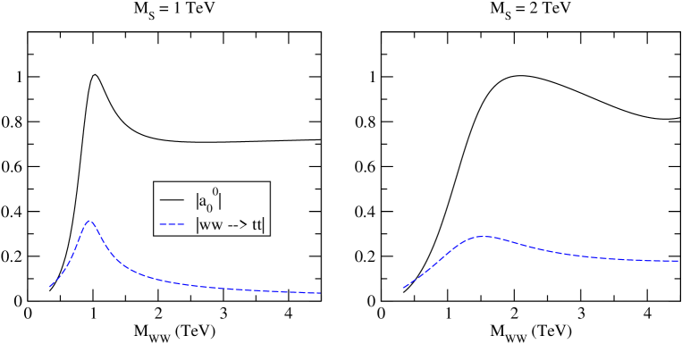
Figure 1.: Unitarity constraints for heavy Scalars. In (a) we show a Higgs-like 1 TeV scalar with $\Gamma(S\rightarrow WW)=493$ GeV and $\Gamma(S\rightarrow t\bar{t})=50$ GeV, whereas in (b) we show a model with a broad enhancement in the $I=J=0$ channel corresponding to parameters $M_{S}=2$ TeV, $g_{S}=0.9$ and $\kappa=1.35$. In both cases perturbative unitarity is satisfied up to 4 TeV.

For the vector resonance the inelastic process $ww\to t\bar{t}$ satisfies the unitarity constraint in all cases once we impose the low energy constraint, Eq. (9). However, there are two partial waves in $ww$ scattering that could be problematic [22] in this case. We demand that $|a^{0}_{0}|\leq 1$ and that $|a^{1}_{1}|\leq 1$, which using the Equivalence Theorem correspond to:

$$|a^{0}_{0}(s)|=\left|{s\over 16\pi v^{2}}+6{\Gamma_{W}\over M_{V}}\left[\left(2+{M_{V}^{2}\over s}\right)\log\left(1+{s\over M_{V}^{2}}\right)-1-{3s\over 2M_{V}^{2}}\right]\right|\;<\;1\;,$$ (13)

and

$$|a^{1}_{1}(s)| = \left|{s\over 96\pi v^{2}}+i\,{\Gamma_{W}^{2}s\over(s-M_{V}^{2})+\Gamma_{W}^{2}M_{V}^{2}}+3{\Gamma_{W}\over M_{V}}\left(1+2{M_{V}^{2}\over s}\right)\left(2+{M_{V}^{2}\over s}\right)\log\left(1+{s\over M_{V}^{2}}\right)\right.$$ (14)

$$- \left.{{\Gamma_{W}\over M_{V}}\over(s-M_{V}^{2})+\Gamma_{W}^{2}M_{V}^{2}}\left[6{M_{V}^{6}\over s}+{3s^{3}\over 2M_{V}^{2}}+10s^{2}-{35\over 2}sM_{V}^{2}\right]+\cdots\right|\;<\;1.$$ (15)

In this second expression we have not written down terms of higher order in $\Gamma_{W}/M_{V}$, which we have denoted by the ellipses. Examples of parameters satisfying both conditions for a 1 and 2 TeV vector resonance are shown in Fig. 2. For the 1 TeV resonance we use $\tilde{g}=3$ and $g_{V}=-g_{A}=0.09$ which correspond to $\Gamma(V\rightarrow WW)=50$ GeV and $\Gamma(V\rightarrow t\bar{t})=1.3$ GeV. For the case $M_{V}=2$ TeV we choose $\tilde{g}=5.38$ and $g_{V}=-g_{A}=0.16$, corresponding to $\Gamma(V\rightarrow WW)=500$ GeV and $\Gamma(V\rightarrow t\bar{t})=8.2$ GeV respectively. We have chosen both of these resonances to be relatively narrow. Notice also that the width into $t\bar{t}$ induced by the direct coupling is almost two orders of magnitude larger than the one induced by mixing. Finally we point out that the vector is sufficiently narrow to simply use a constant width for the $s$-channel vector propagator.

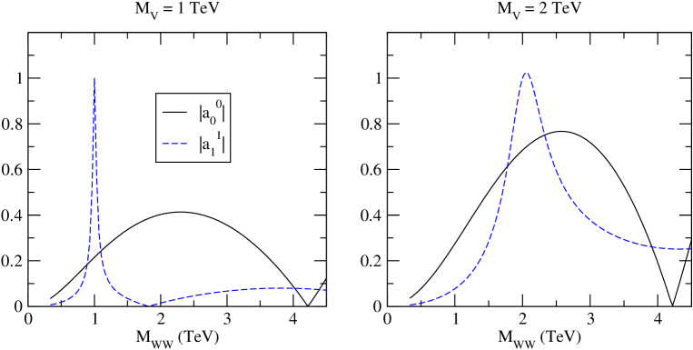
Figure 2.: Unitarity constraints for heavy Vectors. In (a) we show a 1 TeV vector with $\Gamma(V\rightarrow WW)=50$ GeV and $\Gamma(V\rightarrow t\bar{t})=1.3$ GeV, whereas in (b) we show a 2 TeV vector with $\Gamma(V\rightarrow WW)=500$ GeV and $\Gamma(V\rightarrow t\bar{t})=8.2$ GeV. In both cases perturbative unitarity is satisfied up to 4 TeV.

As argued above, it is not possible to have a heavy and narrow scalar unless there are additional ingredients in the model. Simple models that can be constructed may include additional light scalars or additional resonances. Here we present two simple examples including only one scalar and one vector resonance. In Fig. 3 we illustrate two choices of parameters that satisfy all the unitarity conditions that we have discussed. The first one has a 2 TeV scalar with a 1 TeV vector and couplings $g_{S}=0.3$, $\tilde{g}=3$, $\kappa=1$ and $g_{V}=0.09$. This translates into $\Gamma(S\rightarrow WW)=355$ GeV, $\Gamma(V\rightarrow WW)=50$ GeV, $\Gamma(S\rightarrow t\bar{t})=114$ GeV, and $\Gamma(V\rightarrow t\bar{t})=1.3$ GeV. In the second example we chose $M_{S}=1$ TeV and $M_{V}=2$ TeV with $g_{S}=0.8$, $\tilde{g}=15.5$, $\kappa=1$ and $g_{V}=0.43$. This leads to $\Gamma(S\rightarrow WW)=315$ GeV, $\Gamma(V\rightarrow WW)=60$ GeV, $\Gamma(S\rightarrow t\bar{t})=50$ GeV, and $\Gamma(V\rightarrow t\bar{t})=60$ GeV.

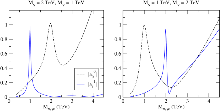
Figure 3.: Models with two resonances that satisfy the perturbative unitarity constraints with parameters described in the text.

IV Sensitivity to the Top-SEWS Signal at the LHC

Clearly, one direct way of probing enhanced electroweak couplings to the top quark at the LHC is $t\bar{t}$ production via weak boson fusion. Although gluon fusion via heavy quark loops typically leads to a larger production rate for a scalar resonance, the gauge boson fusion processes may be more advantageous because of the enhanced gauge boson coupling to new physics, as well as advantages of the final state kinematics, which have been used previously in studies of intermediate mass and heavy Higgs bosons at hadron colliders [13, 23, 6]. In fact, there is no viable technique to make use of the gluon-fusion channel for a heavy Higgs signal $H\to t\bar{t}$ due to the overwhelming background $gg,q\bar{q}\to t\bar{t}$. We thus concentrate on the $W$-fusion channel and explore its observability. For a careful study of the background we must include all EW Feynman graphs for pair production of two top quarks and two additional light partons, $qq^{\prime}\to q^{\prime\prime}q^{\prime\prime\prime}t\bar{t}$.

We first consider SM heavy Higgs production and decay to a top quark pair, for Higgs boson mass values $M_{H}=360,800$ GeV. This provides a baseline for comparison of non-SM scenarios with SM expectations. Next we consider two different heavy non-SM scalar resonances, $M_{S}=1.0,2.0$ TeV, for which the Feynman diagrams mentioned above apply, but with enhanced couplings (magnitude) of the scalar to weak bosons and top quarks as discussed in Sec. II. We then consider production of vector states for $M_{V}=1.0,2.0$ TeV, for which the Feynman diagrams still contain a Higgs scalar with $M_{H}\to\infty$ (set to $10^{8}$ GeV in practice) in addition to the new vector resonance graphs, and finally the 2 TeV vector case of the last model considered, consisting of both a heavy non-SM scalar and vector. The $M_{H}\to\infty$ terms are used to reproduce the low energy theorems of the effective theory and are only needed in the case of the heavy vector. Our formulation of the heavy scalar already includes those terms (also applied to the last model).

The major background to any of these potential signals is SM QCD production of $t\bar{t}$ plus two partons, “$t\bar{t}jj$”, which has been described elsewhere [13] as one of the dominant SM backgrounds that LHC Higgs searches will face. Before stronger cuts are imposed on the forward partons, a total cross section for this background is not easy to obtain, as the calculation experiences soft and collinear singularities of the additional partons. The limiting case would of course be the total $t\bar{t}$ cross section, where the emission of additional soft or collinear partons is not observed.

Table I shows the model parameters used for each resonance considered, their resulting total widths, LHC production cross sections without kinematic cuts or decays, and cross sections with decays and cuts required for detector observation (discussed in detail below). Notice that the widths in this Table do not agree exactly with what we say in Sec. II. The differences arise from the additional electroweak strength terms in the numerical implementation as compared to the widths calculated in Sec. II with the aid of the Equivalence Theorem. Our numerical estimates do not use the equivalence theorem. For the scalar resonance they correspond to an exact tree-level calculation with the model defined by Eqs. 1 and 3. For the vector resonance we assume that the direct $s$-channel exchange of the new resonance dominates, and that the direct coupling of the resonance to $t\bar{t}$ is larger than the mixing-induced coupling. For the cross section without decays or cuts, we restrict the kinematic range of the two forward scattered quarks to $p_{T}>10$ GeV, to avoid collinear singularities in the background calculations.

TABLE I.: Model parameters, total widths and resultant total cross sections for the SM Higgs boson, non-SM scalar and non-SM vector resonances considered. Parameters are chosen to maximize the cross section without violating the unitarity constraints derived in Sec. II. In addition we show the QCD $t\bar{t}jj$ continuum. All cross sections are without decay of the top quarks. We include kinematic cuts on the two scattered far forward scattered partons as described in the text, to make the calculations stable against soft and collinear singularities. The QCD top quark background is uncertain to a factor of several at this stage, due to the scattered partons being well into the non-perturbative region of QCD for this level of cuts.

state	$M$ (GeV)	$g_{S},\kappa$	$\tilde{g},g_{V}$	$\Gamma$ (GeV)	$\sigma_{``tot^{\prime\prime}}$ (fb)	$\sigma_{dec/cuts}$ (fb)
SM $H$	360	-,-	-,-	17.6	29.0	1.40
SM $H$	800	-,-	-,-	308	25.3	1.56
$S$	1000	1.0 ,1.0	-,-	519	21.2	1.25
$S$	2000	0.9 ,1.35	-,-	3339	16.5	0.86
$V$	1000	-,-	3.0 ,0.09	51.6	18.0	0.97
$V$	2000	-,-	5.38,0.16	507	13.2	0.84
$S+V$	1000,2000	0.8,1.0	15.5,0.43	349,119	20.5	1.33
QCD $t\bar{t}jj$	-	-,-	-,-	-	few $\times 10^{5}$	7200

Unfortunately, the background cross section is several orders of magnitude larger than any of the signal processes we consider. To determine if there is any hope of extracting a signal from this extremely large QCD continuum, we must consider specific final state signatures. Dual hadronic decay of the top quarks constitutes the largest branching ratio, about $45\%$, and yields an eight jet final state, of which two (typically central) jets are bottom quarks, and two light jets are required to be found very far forward. Unfortunately there is a question as to whether such all-jet final states can be accepted by the trigger due to their large rate, so we do not consider this channel. Instead, we analyze semi-leptonic decay of the top quark pair, which has a $29\%$ branching ratio and yields two far forward/backward light jets, two central $b$ jets, two central light jets which could be reconstructed to a $W$ boson, a central lepton (only $e$ or $\mu$ is considered), and significant missing transverse energy. To make the simulation more realistic we impose Gaussian smearing to the final state particles’ momenta according to CMS expectations [24].

For this final state we impose first the minimum set of kinematic cuts that will be required for detector acceptance and identification of the final state:

$$p_{T}(j)>20~{}{\rm GeV},\qquad p_{T}(b)>20~{}{\rm GeV},\qquad p_{T}(\ell)>15~{}{\rm GeV},$$ (16)

$$|\eta(j)|<4.5\;,\qquad\qquad|\eta(b)|<2.5\;,\qquad\qquad|\eta(\ell)|<2.5\;,$$ (17)

$$\Delta R(jj,jb,bb)>0.4\;,\qquad\Delta R(j\ell)>0.4\;,\qquad\Delta R(\ell\ell)>0.2\;,$$ (18)

$$/\!\!\!p_{T}>30~{}{\rm GeV}.$$ (19)

We also immediately apply the basic “rapidity gap” cuts well established in [13], which reduces the various signals by a typical factor 4, and the background in this case by about an order of magnitude:

$$\eta_{j,min}+0.6<\eta_{\ell_{1,2}}<\eta_{j,max}-0.6\,,$$ (20)

$$\eta_{j_{1}}\cdot\eta_{j_{2}}<0\,,\qquad\triangle\eta_{tags}=|\eta_{j_{1}}-\eta_{j_{2}}|\geq 4.2\,,$$ (21)

leaving a gap of at least 3 units of pseudo-rapidity in which the charged lepton, $b$ jets and $W$ boson decay jets can be observed. Given four jets in the final state, not counting additional QCD radiation, there must be some criteria to select which two will be the forward tagging jets. We find that to a very high efficiency, typically on the order of $90\%$ or better, selection of the two most energetic jets fulfills this requirement. If instead the two highest $p_{T}$ jets are chosen, the cross section drops by a factor of four, due to one of the jets from the hadronic $W$ boson being chosen as a tagging jet candidate. The event in those cases rarely satisfies the requirement that all other final state particles lie in the rapidity region between the tagging jets. With these cuts imposed, the various signals have resulting cross sections all at around the 1 fb level, as shown in Table I. However, the QCD background is a factor 7000 larger. Clearly this is far too much to have any hope of observing any of the signals.

An estimate of the reduction factor necessary for signal observation can be obtained by calculating the maximum number of background events allowable for, say, a $5\sigma$ statistical significance, given the likely number of signal events in 300 fb^-1 of data. To be realistic we apply two factors of 0.5 for the probability to tag the two $b$ quark jets, two factors of $68\%$ for the expected efficiency to identify the forward tagging jets, and a $90\%$ lepton ID efficiency. We ignore the loss of signal that comes from reconstructing the hadronic $W$ boson, or its parent top quark (one might argue this is not necessary given the complex final state signature). This leaves us with on the order of 30 signal events, or an allowable background of about 40 events – a factor 6000 reduction of the QCD background.

Figure 4.: Invariant mass of the forward tagging jets at the LHC, selected as the two highest energy jets in the event. The SM Higgs boson signals for $M_{H}=360,800$ GeV are shown by the dashed curves, the two non-SM scalar cases by the solid curves, the non-SM heavy vectors by the dashed curves, and the QCD continuum by the dot-dashed curve.

Figure 5.: Transverse mass (a) and generated invariant mass (b) of the top quark pair at the LHC. The SM Higgs boson signals for $M_{H}=360,800$ GeV are shown by the dashed curves, the two non-SM scalar cases by the solid curves, and the QCD continuum by the dot-dashed curve. Note that panel (b) does not represent a realistic observable.

Figure 6.: Transverse mass (a) and generated invariant mass (b) of the top quark pair at the LHC. The non-SM heavy vectors are shown by the dashed curves, the non-SM scalar+vector case by the dashed curve, and the QCD continuum by the dot-dashed curve. Note that panel (b) does not represent a realistic observable.

There are a few obvious possibilities to pursue. The first is to cut on the invariant mass of the forward tagging jets, a standard technique [13]. We show the various signal and QCD background $m_{jj}^{\rm tags}$ in Fig. 4. For example, a cut of $m_{jj}^{\rm tags}>1$ TeV would reduce any of the signals by about $1/4$, but the QCD background by only about $3/4$, clearly not a significant gain. Another possibility is to look for the resonance peak of the top quark pair due to the new scalar or vector state. Unfortunately, because of the single leptonic top quark decay and resulting neutrino that escapes the detector, the top quark pair cannot be completely reconstructed. But one can determine the transverse mass of the top quark pair, which is almost as good.

We plot $m_{T}(t\bar{t})$ in Figs. 5(a), 6(a) for the various signals and QCD background. It becomes immediately apparent that a peak beyond the electroweak continuum exists only for a relatively light state, close to $2m_{t}$, and the comparatively very narrow 1 TeV vector resonance. The reasons for this are a combination of effects. First, the very large widths of the states smear out the resonances into the EW continuum. Second, detector effects cause mismeasurement of the events which smear out the transverse mass peaks to the point of indistinguishability. We verify this by plotting the generated top quark pair invariant mass in Figs. 5(b) and 6(b), which would be the ideal variable for the signal search if it were reconstructible. There are no visible resonance peaks for the heavy, wide states in this distribution, although the heavy narrow states do have a peak above the EW continuum. Third, for the 2 TeV narrow state considered in the last model, jet separation cuts remove almost all the events, as the highly boosted top quark decay into very narrow, massive jets. More detailed Monte Carlo simulations and different techniques need to be developed in order to discriminate these kinds of new physics events from SM backgrounds, which is beyond the scope of the current study.

One might hope to use the upper end of a distribution, if not an actual peak, for the more massive states. Unfortunately, the QCD background has an extremely broad continuum distribution in $m_{T}(t\bar{t})$, similar to the EW continuum, and there is almost no event rate left in this tail, so this does not appear to be possible at the LHC. Even for the case where some vestige of a peak exists, the signal cannot stand out against the overwhelming QCD continuum. One is simply at the mercy of QCD production of the same massive final state.

Figure 7.: Transverse mass (a) and generated invariant mass (b) of the top quark pair at a VLHC. The SM Higgs boson signals for $M_{H}=360,800$ GeV are shown by the dashed curves, the two non-SM scalar cases by the solid curves, and the QCD continuum by the dot-dashed curve. Note that panel (b) does not represent a realistic observable.

Figure 8.: Transverse mass (a) and generated invariant mass (b) of the top quark pair at a VLHC. The non-SM heavy vectors are shown by the dashed curves, the non-SM scalar+vector case by the dashed curve, and the QCD continuum by the dot-dashed curve. Note that panel (b) does not represent a realistic observable.

One could consider the opportunity of a VLHC instead, $pp$ collisions at $\sqrt{s}=200$ TeV. For these energies we increase the kinematic cut thresholds to avoid an expected large jet multiplicity at low $p_{T}$: we require $p_{T}(j,tag)>40$ GeV and $p_{T}(b,j)>30$ GeV. At 200 TeV the QCD continuum increases by a factor 30, to 230 pb in the semi-leptonic decay channel. However, the SM Higgs boson signal for example increases by only a factor 10 for $M_{H}=360$ GeV, to 14.4 fb, and a factor 14 for $M_{H}=800$ GeV, to 22.0 fb. The non-SM heavy resonances have similar cross sections, eliminating the possibility of any gain there as well. We again show the transverse mass of the top quark pair in Figs. 7(a), 8(a). As this continuum will exhibit the same broad distribution at a much higher energy VLHC, we conclude that the massive TOP-SEWS states and their subsequent decay to top quarks are not likely to be a viable channel to observe at the VLHC.

V Conclusion

Given the high energy and luminosity achievable at future hadron colliders, and the fact that the LHC will be in its mission in the near future, it would be important to quantify to what extent the physics of a novel electroweak symmetry breaking sector that strongly couples to the top-quark sector can be explored. We constructed models for heavy scalar and vector resonances with large couplings to top quarks and electroweak gauge bosons that respect unitarity in the energy region probed by the LHC. We computed the rates for the processes $qq^{\prime}\to q^{\prime\prime}q^{\prime\prime\prime}t\bar{t}$ via gauge-boson fusion mediated by these resonances without making approximation for the gauge bosons, and studied whether these processes would be observable at the LHC or the VLHC. We find that in all cases the signals are completely swamped by QCD backgrounds. A simple way to understand this is that our models produced in all cases event rates of the same order of magnitude of that one obtains by simply using a heavy SM Higgs boson. Unfortunately, the QCD background gives rates that are larger by more than three orders of magnitude, making it impossible to extract the signal. No sharp peak in any reconstructible distribution can be observed as a result of smearing out from missing energy and detector effects.

We have also considered the possible production of a vector state via the direct $q\bar{q}$ annihilation. Since the direct coupling of such a vector state to light fermions is constrained to be negligibly small [15], we considered production through the $\gamma/Z-V$ mixing induced couplings as given in Ref. [15]. Unfortunately, the signal cross sections turn out to be very small. For the two cases under our consideration, we obtained the production cross section via $q\bar{q}\rightarrow\gamma/Z-V\rightarrow t\bar{t}$ to be about 3 (130) fb for $M_{V}=1$ TeV, and about 0.02 (2.3) fb for $M_{V}=2$ TeV at the LHC (VLHC) energies, which are too small to be significant.

As a final note, the TOP-SEWS models under consideration often have charged heavy scalar or vector states in addition to the heavy neutral states. It would be desirable to observe these states via decay to a single top quark. In this case the most obvious background is single top quark production, which is an electroweak process. However, the leading cross section comes from $Wb\to t$ fusion and the rate is smaller than QCD $t\bar{t}$ production only by about a factor of three at LHC energy [25]. Even the $t\bar{t}+jets$ production will be a background, when some of the decay products are lost. The signal for charged (color singlet) resonances at the TeV region does not look more promising than that for the neutral resonant states as studied in this paper. We therefore have not considered the charged states in more detail.

Future hadron colliders such as the LHC or VLHC are truly top-quark factories, with $\approx 250$ million $t\bar{t}$ events produced for instance at the LHC per 300 fb^-1 luminosity. Ironically, this large top-quark cross section from QCD becomes the major obstacle for studying the possible novel electroweak symmetry-breaking physics associated with the top quark. In contrast, lepton colliders with a c.m. energy of 1.5 TeV or higher would have the potential to explore this class of electroweak physics, and to determine the leading partial decay widths of the new states (which characterize the coupling strengths) statistically to about $10\%$ [12].

Acknowledgments: The work of T.H. was supported in part by the US DOE under contract No. DE-FG02-95ER40896 and in part by the Wisconsin Alumni Research Foundation. The work of G.V. was supported in part by DOE under contact number DE-FG02-01ER41155. We would also like to thanks the organizers of the Snowmass 2001 workshop, where part of this work was conducted.

Bibliography

- [1] M. S. Chanowitz, Ann. Rev. Nucl. Part. Sci. 38, 323 (1988); For a recent review on dynamical models, see e. g., C. Hill and E. Simmons, arXiv:hep-ph/0203079.
- [2] M. S. Chanowitz, Phys. Rev. Lett. 87, 231802 (2001).
- [3] M. S. Chanowitz, Phys. Rev. D 66, 073002 (2002) [arXiv:hep-ph/0207123].
- [4] M. E. Peskin and J. D. Wells, Phys. Rev. D64, 093003 (2001).
- [5] R. S. Chivukula, C. Hoelbling and N. Evans, Phys. Rev. Lett. 85, 511 (2000) [arXiv:hep-ph/0002022].
- [6] J. Bagger et al., Phys. Rev. D49, 1246 (1994); ibid. D52, 3878 (1995).
- [7] C. T. Hill, Phys. Lett. B266, 419 (1991); ibid. B345, 483 (1995); C. T. Hill and S. J. Parke, Phys. Rev. D 49, 4454 (1994); E. Eichten and K. Lane, Phys. Lett. B352, 382 (1995).
- [8] B. Dobrescu and C. Hill, Phys. Rev. Lett. 81, 2634 (1998); R. S. Chivukula, B. Dobrescu, H. Georgi, and C. T. Hill, Phys. Rev. D59, 075003 (1999); G. Burdman and N. Evans, Phys. Rev. D59, 115005 (1999); H.-J. He, T. Tait and C.-P. Yuan, Phys. Rev. D62, 011702R (2000); H. J. He, C. T. Hill and T. M. Tait, Phys. Rev. D 65, 055006 (2002).
- [9] E. H. Simmons, hep-ph/9908488.
- [10] F. Larios, E. Malkawi, and C.P. Yuan, Acta Phys. Polon. B27, 3741 (1996); F. Larios, E. Malkawi, and C.P. Yuan, Phys. Rev. D55, 7218 (1997).
- [11] T.L. Barklow, in Proc. of New Directions for High-Energy Physics (Snowmass 96), Snowmass, June 25 – July 12, 1996; F. Larios, Tim Tait, and C.P. Yuan, Phys. Rev. D57 3106 (1998).
- [12] T. Han, Y. J. Kim, A. Likhoded and G. Valencia, Nucl. Phys. B593, 415 (2001).
- [13] D. Rainwater and D. Zeppenfeld, Phys. Rev. D60, 113004 (1999); and references therein.
- [14] Several reviews exist in the literature, for example, M. Golden, T. Han and G. Valencia, arXiv:hep-ph/9511206; R. S. Chivukula, M. J. Dugan, M. Golden and E. H. Simmons, Ann. Rev. Nucl. Part. Sci. 45, 255 (1995) [arXiv:hep-ph/9503230];.
- [15] D. Dominici, Riv. Nuovo Cim. 20, 1 (1997).
- [16] B. W. Lee, C. Quigg, and H. B. Thacker, Phys. Rev. D16, 1519 (1977); M. S. Chanowitz and M. K. Gaillard, Nucl. Phys. B261, 379 (1985).
- [17] J. Bagger, S. Dawson and G. Valencia, JHU-TIPAC-91-002, Snowmass Summer Study 1990, p. 216; J. Bagger, S. Dawson and G. Valencia, Nucl. Phys. B399, 364 (1993).
- [18] J. Bagger, T. Han and R. Rosenfeld, FERMILAB-CONF-90-253-T, published in Snowmass Summer Study 1990, p. 208.
- [19] R. Casalbuoni et al., Phys. Lett. B155, 95 (1985); Nucl. Phys. B282, 235 (1987); B310, 181 (1988); Phys. Lett. B249, 130 (1990); B253, 275 (1991).
- [20] W. Marciano, G. Valencia and S. Willenbrock, Phys. Rev. D40, 1725 (1989).
- [21] M. H. Seymour, Phys. Lett. B354, 409 (1995).
- [22] J. F. Donoghue, C. Ramirez and G. Valencia, Phys. Rev. D 38, 2195 (1988); J. F. Donoghue, C. Ramirez and G. Valencia, Phys. Rev. D 39, 1947 (1989).
- [23] V. Barger, K. Cheung, T. Han and R.J.N. Phillips, Phys. Rev. D42, 3052 (1990).
- [24] CMS TP, report CERN/LHCC/94-38 (1994).
- [25] T. Stelzer, Z. Sullivan, and S. Willenbrock, Phys. Rev. D56, 5919 (1997); M. Beneke et al., arXiv:hep-ph/0003033.