Renormalization of Coupling Constants in the Minimal SUSY Models

Abstract

The considerable part of the parameter space in the MSSM corresponding to the infrared quasi fixed point scenario is excluded by LEP II bounds on the lightest Higgs boson mass. In the NMSSM the mass of the lightest Higgs boson reaches its maximum value in the strong Yukawa coupling limit when Yukawa couplings are essentially larger than gauge ones at the Grand Unification scale. In this case the renormalization group flow of Yukawa couplings and soft SUSY breaking terms is investigated. The quasi–fixed and invariant lines and surfaces are briefly discussed. The coordinates of the quasi–fixed points, where all solutions are concentrated, are given.

Abstract

We review our recent development of family replicated gauge group model, which generates the Large Mixing Angle MSW solution. The model is based on each family of quarks and leptons having its own set of gauge fields, each containing a replica of the Standard Model gauge fields plus a $(B-L)$-coupled gauge field. A fit of all the seventeen quark-lepton mass and mixing angle observables, using just six new Higgs field vacuum expectation values, agrees with the experimental data order of magnitudewise. However, this model can not predict the baryogenesis in right order, therefore, we discuss further modification of our model and present a preliminary result of baryon number to entropy ratio.

Abstract

In our model with a Standard Model gauge group extended with a baryon number minus lepton number charge for each family of quarks and leptons, we calculate the baryon number relative to entropy produced in early Big Bang by the Fukugita-Yanagida mechanism. With the parameters, i.e., the Higgs VEVs already fitted in a very successful way to quark and lepton masses and mixing angles we obtain the order of magnitude pure prediction $Y_{B}=2.59{+17.0\atop-2.25}\times 10^{-11}$ which according to a theoretical estimate should mean in this case an uncertainty of the order of a factor 7 up or down (to be compared to $Y_{B}=(1.7-8.1)\times 10^{-11}$) using a relatively crude approximation for the dilution factor, while using another estimate based on Buchmüller and Plümacher a factor $500$ less, but this should rather be considered a lower limit. With a realistic uncertainty due to wash-out of a factor $100$ up or down we even with the low estimate only deviate by $1.5\sigma$.

Abstract

Vacuum neutrino oscillations for three generations are considered. The influence of the leptonic CP-violating phase (similar to the quarks CP-phase) on neutrino oscillations is taken into account in the matrix of leptons mixing. The dependence of probabilities of a transition of one kind neutrino to another kind on three mixing angles and on the CP-phase is obtained in a general form. It is pointed that one can reconstruct the value of the leptonic CP-phase by measuring probabilities for a transition of one kind neutrino to another kind averaging over all oscillations. Also it is noted that the manifestation of the CP-phase in deviations of probabilities of forward neutrino transitions from probabilities of backward neutrino transitions is an effect practically slipping from an observation.

Abstract

We show that neutral fermions may have an additional source of time reversal violation by associating time reversal with gauge group representations of fermions through the method of group extensions as in the case of parity. This provides a new source of time reversal violation for neutral particles.

1 Introduction

The search for the Higgs boson remains one of the top priorities for existing accelerators as well as for those still at the design stage. This is because this boson plays a key role in the Standard Model which describes all currently available experimental data with a high degree of accuracy. As a result of the spontaneous symmetry breaking $SU(2)\otimes U(1)$ the Higgs scalar acquires a nonzero vacuum expectation value without destroying the Lorentz invariance, and generates the masses of all fermions and vector bosons. An analysis of the experimental data using the Standard Model has shown that there is a $95\%$ probability that its mass will not exceed $210\text{~{}GeV}$ A1 . At the same time, assuming that there are no new fields and interactions and also no Landau pole in the solution of the renormalization group equations for the self-action constant of Higgs fields up to the scale $M_{\text{Pl}}\approx 2.4\cdot 10^{18}\text{~{}GeV}$, we can show that $m_{h}<180\text{~{}GeV}$ A2 ,A3 . In this case, physical vacuum is only stable provided that the mass of the Higgs boson is greater than $135\text{~{}GeV}$ A2 -A6 . However, it should be noted that this simplified model does not lead to unification of the gauge constants A7 and a solution of the hierarchy problem A8 . As a result, the construction of a realistic theory which combines all the fields and interactions is extremely difficult in this case.

Unification of the gauge constants occurs naturally on the scale $M_{X}\approx 3\cdot 10^{16}\text{~{}GeV}$ within the supersymmetric generalisation of the Standard Model, i.e., the Minimal Supersymmetric Standard Model (MSSM) A7 . In order that all the fundamental fermions acquire mass in the MSSM, not one but two Higgs doublets $H_{1}$ and $H_{2}$ must be introduced in the theory, each acquiring the nonzero vacuum expectation value $v_{1}$ and $v_{2}$ where $v^{2}=v_{1}^{2}+v_{2}^{2}=(246\text{~{}GeV})^{2}$. The spectrum of the Higgs sector of the MSSM contains four massive states: two CP–even, one CP–odd, and one charged. An important distinguishing feature of the supersymmetric model is the existing of a light Higgs boson in the CP–even sector. The upper bound on its mass is determined to a considerable extent by the value $\tan\beta=v_{2}/v_{1}$. In the tree-level approximation the mass of the lightest Higgs boson in the MSSM does not exceed the mass of the Z-boson ($M_{Z}\approx 91.2\text{~{}GeV}$): $m_{h}\leq M_{Z}|\cos 2\beta|$ A9 . Allowance for the contribution of loop corrections to the effective interaction potential of the Higgs fields from a $t$–quark and its superpartners significantly raises the upper bound on its mass:

$$m_{h}\leq\sqrt{M_{Z}^{2}\cos^{2}2\beta+\Delta}\,.$$ (1)

Here $\Delta$ are the loop corrections A10 ,A11 . The values of these corrections are proportional to $m_{t}^{4}$, where $m_{t}$ is the running mass of $t$–quark which depends logarithmically on the supersymmetry breaking scale $M_{S}$ and is almost independent of the choice of $\tan\beta$. In A3 ,A5 ,A6 bounds on the mass of the Higgs boson were compared in the Minimal Standard and Supersymmetric models. The upper bound on the mass of the light CP–even Higgs boson in the MSSM increases with increasing $\tan\beta$ and for $\tan\beta\gg 1$ in realistic supersymmetric models with $M_{S}\leq 1000\text{~{}GeV}$ reaches $125-128\text{~{}GeV}$.

However, a considerable fraction of the solutions of the system of MSSM renormalization group equations is focused near the infrared quasi-fixed point at $\tan\beta\sim 1$. In the region of parameter space of interest to us ($\tan\beta\ll 50$) the Yukawa constants of a $b$–quark ($h_{b}$) and a $\tau$–lepton ($h_{\tau}$) are negligible so that an exact analytic solution can be obtained for the one–loop renormalization group equations A12 . For the Yukawa constants of a $t$–quark $h_{t}(t)$ and the gauge constants $g_{i}(t)$ its solution has the following form:

$$\begin{gathered}Y_{t}(t)=\frac{\dfrac{E(t)}{6F(t)}}{1+\dfrac{1}{6Y_{t}(0)F(t)}},\quad\tilde{\alpha}_{i}(t)=\frac{\tilde{\alpha}_{i}(0)}{1+b_{i}\tilde{\alpha}_{i}(0)t},\\ E(t)=\left[\frac{\tilde{\alpha}_{3}(t)}{\tilde{\alpha}_{3}(0)}\right]^{16/9}\left[\frac{\tilde{\alpha}_{2}(t)}{\tilde{\alpha}_{2}(0)}\right]^{-3}\left[\frac{\tilde{\alpha}_{1}(t)}{\tilde{\alpha}_{1}(0)}\right]^{-13/99},\quad F(t)=\int\limits_{0}^{t}E(t^{\prime})dt^{\prime},\end{gathered}$$ (2)

where the index $i$ has values between 1 and 3,

$$b_{1}=33/5,\quad b_{2}=1,\quad b_{3}=-3$$

$$\tilde{\alpha}_{i}(t)=\left(\frac{g_{i}(t)}{4\pi}\right)^{2},\quad Y_{i}(t)=\left(\frac{h_{t}(t)}{4\pi}\right)^{2}.$$

The variable $t$ is determined by a standard method $t=\ln(M_{X}^{2}/q^{2})$. The boundary conditions for the renormalization group equations are usually set at the grand unification scale $M_{X}$ ($t=0$) where the values of all three Yukawa constants are the same: $\tilde{\alpha}_{1}(0)=\tilde{\alpha}_{2}(0)=\tilde{\alpha}_{3}(0)=\tilde{\alpha}_{0}.$ On the electroweak scale where $h_{t}^{2}(0)\gg 1$ the second term in the denominator of the expression describing the evolution of $Y_{t}(t)$ is much smaller than unity and all the solutions are concentrated in a narrow interval near the quasi-fixed point $Y_{\text{QFP}}(t)=E(t)/6F(t)$ A13 . In other words in the low-energy range the dependence of $Y_{t}(t)$ on the initial conditions on the scale $M_{X}$ disappears. In addition to the Yukawa constant of the $t$–quark, the corresponding trilinear interaction constant of the scalar fields $A_{t}$ and the combination of the scalar masses $\mathfrak{M}^{2}_{t}=m_{Q}^{2}+m_{U}^{2}+m_{2}^{2}$ also cease to depend on $A_{t}(0)$ and $\mathfrak{M}_{t}^{2}(0)$ as $Y_{t}(0)$ increases. Then on the electroweak scale near the infrared quasi–fixed point $A_{t}(t)$ and $\mathfrak{M}_{t}^{2}(t)$ are only expressed in terms of the gaugino mass on the Grand Unification scale. Formally this type of solution can be obtained if $Y_{t}(0)$ is made to go to infinity. Deviations from this solution are determined by ratio $1/6F(t)Y_{t}(0)$ which is of the order of $1/10h_{t}^{2}(0)$ on the electroweak scale.

The properties of the solutions of the system of MSSM renormalization group equations and also the particle spectrum near the infrared quasi-fixed point for $\tan\beta\sim 1$ have been studied by many authors A14 ,A15 . Recent investigations A15 -A17 have shown that for solutions $Y_{t}(t)$ corresponding to the quasi-fixed point regime the value of $\tan\beta$ is between $1.3$ and $1.8$. These comparatively low values of $\tan\beta$ yield significantly more stringent bounds on the mass of the lightest Higgs boson. The weak dependence of the soft supersymmetry breaking parameters $A_{t}(t)$ and $\mathfrak{M}_{t}^{2}(t)$ on the boundary conditions near the quasi-fixed point means that the upper bound on its mass can be calculated fairly accurately. A theoretical analysis made in A15 ,A16 showed that $m_{h}$ does not exceed $94\pm 5\text{~{}GeV}$. This bound is $25-30\text{~{}GeV}$ below the absolute upper bound in the Minimal Supersymmetric Model. Since the lower bound on the mass of the Higgs boson from LEP II data is $113\text{~{}GeV}$ A1 , which for the spectrum of heavy supersymmetric particles is the same as the corresponding bound on the mass of the Higgs boson in the Standard Model, a considerable fraction of the solutions which come out to a quasi–fixed point in the MSSM, are almost eliminated by existing experimental data. This provides the stimulus for theoretical analyses of the Higgs sector in more complex supersymmetric models.

The simplest expansion of the MSSM which can conserve the unification of the gauge constants and raise the upper bound on the mass of the lightest Higgs boson is the Next–to–Minimal Supersymmetric Standard Model (NMSSM) A18 -A20 . By definition the superpotential of the NMSSM is invariant with respect to the discrete transformations $y^{\prime}_{\alpha}=e^{2\pi i/3}y_{\alpha}$ of the $Z_{3}$ group A19 which means that we can avoid the problem of the $\mu$-term in supergravity models. The thing is that the fundamental parameter $\mu$ should be of the order of $M_{\text{Pl}}$ since this scale is the only dimensional parameter characterising the hidden (gravity) sector of the theory. In this case, however, the Higgs bosons $H_{1}$ and $H_{2}$ acquire an enormous mass $m^{2}_{H_{1},H_{2}}\sim\mu^{2}\sim M^{2}_{\text{Pl}}$ and no breaking of $SU(2)\otimes U(1)$ symmetry occurs. In the NMSSM the term $\mu(\hat{H}_{1}\hat{H}_{2})$ in the superpotential is not invariant with respect to discrete transformations of the $Z_{3}$ group and for this reason should be eliminated from the analysis ($\mu=0$). As a result of the multiplicative nature of the renormalization of this parameter, the term $\mu(q)$ remains zero on any scale $q\leq M_{X}\div M_{\text{Pl}}$. However, the absence of mixing of the Higgs doublets on electroweak scale has the result that $H_{1}$ acquires no vacuum expectation value as a result of the spontaneous symmetry breaking and $d$–type quarks and charged leptons remain massless. In order to ensure that all quarks and charged leptons acquire nonzero masses, an additional singlet superfield $\hat{Y}$ with respect to gauge $SU(2)\otimes U(1)$ transformations is introduced in the NMSSM. The superpotential of the Higgs sector of the Nonminimal Supersymmetric Model A18 -A20 has the following form:

$$W_{h}=\lambda\hat{Y}(\hat{H}_{1}\hat{H}_{2})+\frac{\varkappa}{3}\hat{Y}^{3}.$$ (3)

As a result of the spontaneous breaking of $SU(2)\otimes U(1)$ symmetry, the field $Y$ acquires a vacuum expectation value ($\langle Y\rangle=y/\sqrt{2}$) and the effective $\mu$-term ($\mu=\lambda y/\sqrt{2}$) is generated.

In addition to the Yukawa constants $\lambda$ and $\varkappa$, and also the Standard Model constants, the Nonminimal Supersymmetric Model contains a large number of unknown parameters. These are the so-called soft supersymmetry breaking parameters which are required to obtain an acceptable spectrum of superpartners of observable particles form the phenomenological point of view. The hypothesis on the universal nature of these constants on the Grand Unification scale allows us to reduce their number in the NMSSM to three: the mass of all the scalar particles $m_{0}$, the gaugino mass $M_{1/2}$, and the trilinear interaction constant of the scalar fields $A$. In order to avoid strong CP–violation and also spontaneous breaking of gauge symmetry at high energies ($M_{\text{Pl}}\gg E\gg m_{t}$) as a result of which the scalar superpartners of leptons and quarks would require nonzero vacuum expectation values, the complex phases of the soft supersymmetry breaking parameters are assumed to be zero and only positive values of $m_{0}^{2}$ are considered. Naturally universal supersymmetry breaking parameters appear in the minimal supergravity model A31 and also in various string models A29 ,A32 . In the low-energy region the hypothesis of universal fundamental parameters allows to avoid the appearance of neutral currents with flavour changes and can simplify the analysis of the particle spectrum as far as possible. The fundamental parameters thus determined on the Grand Unification scale should be considered as boundary conditions for the system of renormalization group equations which describes the evolution of these constants as far as the electroweak scale or the supersymmetry breaking scale. The complete system of the renormalization group equations of the Nonminimal Supersymmetric Model can be found in A33 , A34 . These experimental data impose various constraints on the NMSSM parameter space which were analysed in A35 ,A36 .

The introduction of the neutral field $Y$ in the NMSSM potential leads to the appearance of a corresponding $F$–term in the interaction potential of the Higgs fields. As a consequence, the upper bound on the mass of the lightest Higgs boson is increased:

$$m_{h}\leq\sqrt{\frac{\lambda^{2}}{2}v^{2}\sin^{2}2\beta+M_{Z}^{2}\cos^{2}2\beta+\Delta^{(1)}_{11}+\Delta^{(2)}_{11}}.$$ (4)

The relationship (4) was obtained in the tree-level approximation ($\Delta_{11}=0$) in A20 . However, loop corrections to the effective interaction potential of the Higgs fields from the $t$–quark and its superpartners play a very significant role. In terms of absolute value their contribution to the upper bound on the mass of the Higgs boson remains approximately the same as in the Minimal Supersymmetric Model. When calculating the corrections $\Delta_{11}^{(1)}$ and $\Delta_{11}^{(2)}$ we need to replace the parameter $\mu$ by $\lambda y/\sqrt{2}$. Studies of the Higgs sector in the Nonminimal Supersymmetric model and the one–loop corrections to it were reported in A24 ,A33 ,A36 -A39 . In A6 the upper bound on the mass of the lightest Higgs boson in the NMSSM was compared with the corresponding bounds on $m_{h}$ in the Minimal Standard and Supersymmetric Models. The possibility of a spontaneous CP–violation in the Higgs sector of the NMSSM was studied in A39 ,A40 .

It follows from condition (4) that the upper bound on $m_{h}$ increases as $\lambda$ increases. Moreover, it only differs substantially from the corresponding bound in the MSSM in the range of small $\tan\beta$. For high values ($\tan\beta\gg 1$) the value of $\sin 2\beta$ tends to zero and the upper bounds on the mass of the lightest Higgs boson in the MSSM and NMSSM are almost the same. The case of small $\tan\beta$ is only achieved for fairly high values of the Yukawa constant of a $t$–quark $h_{t}$ on the electroweak scale ($h_{t}(t_{0})\geq 1$ where $t_{0}=\ln(M_{X}^{2}/m_{t}^{2})$), and $\tan\beta$ decreases with increasing $h_{t}(t_{0})$. However, an analysis of the renormalization group equations in the NMSSM shows that an increase of the Yukawa constants on the electroweak scale is accompanied by an increase of $h_{t}(0)$ and $\lambda(0)$ on the Grand Unification scale. It thus becomes obvious that the upper bound on the mass of the lightest Higgs boson in the Nonminimal Supersymmetric model reaches its maximum on the strong Yukawa coupling limit, i.e., when $h_{t}(0)\gg g_{i}(0)$ and $\lambda(0)\gg g_{i}(0)$.

2 Renormalization of the Yukawa couplings

From the point of view of a renormalization group analysis, investigation of the NMSSM presents a much more complicated problem than investigation of the minimal SUSY model. The full set of renormalization group equations within the NMSSM can be found in A33 ,A34 . Even in the one–loop approximation, this set of equations is nonlinear and its analytic solution does not exist. All equations forming this set can be partitioned into two groups. The first one contains equations that describe the evolution of gauge and Yukawa coupling constants, while the second one includes equations for the parameters of a soft breakdown of SUSY, which are necessary for obtaining a phenomenologically acceptable spectrum of superpartners of observable particles. Since boundary conditions for three Yukawa coupling constants are unknown, it is very difficult to perform a numerical analysis of the equations belonging to the first group and of the full set of the equations given above. In the regime of strong Yukawa coupling, however, solutions to the renormalization group equations are concentrated in a narrow region of the parameter space near the electroweak scale, and this considerably simplifies the analysis of the set of equations being considered.

In analysing the nonlinear differential equations entering into the first group, it is convenient to use the quantities $\rho_{t}$, $\rho_{\lambda}$, $\rho_{\varkappa}$, $\rho_{1}$, and $\rho_{2}$, defined as follows:

$$\rho_{t}(t)=\frac{Y_{t}(t)}{\tilde{\alpha}_{3}(t)},\quad\rho_{\lambda}(t)=\frac{Y_{\lambda}(t)}{\tilde{\alpha}_{3}(t)},\quad\rho_{\varkappa}(t)=\frac{Y_{\varkappa}(t)}{\tilde{\alpha}_{3}(t)},$$

$$\rho_{1}(t)=\frac{\tilde{\alpha}_{1}(t)}{\tilde{\alpha}_{3}(t)},\quad\rho_{2}(t)=\frac{\tilde{\alpha}_{2}(t)}{\tilde{\alpha}_{3}(t)},$$

where $\tilde{\alpha}_{i}(t)=g^{2}_{i}(t)/(4\pi)^{2}$, $Y_{t}(t)=h^{2}_{t}(t)/(4\pi)^{2}$, $Y_{\lambda}(t)=\lambda^{2}(t)/(4\pi)^{2}$, and $Y_{\varkappa}(t)=\varkappa^{2}(t)/(4\pi)^{2}$.

Figure 1: The values of the Yukawa couplings at the electroweak scale corresponding to the initial values at the GUT scale uniformly distributed in a square $2\leq h_{t}^{2}(0),\lambda^{2}(0)\leq 10$. The thick and thin curves represent, respectively, the invariant and the Hill line. The dashed line is a fit of the values $(\rho_{t}(t_{0}),\rho_{\lambda}(t_{0}))$ for $20\leq h_{t}^{2}(0),\lambda^{2}(0)\leq 100$.

Figure 2: The values of the Yukawa couplings at the electroweak scale corresponding to the initial values at the GUT scale uniformly distributed in a square $20\leq h_{t}^{2}(0),\lambda^{2}(0)\leq 100$. The dashed line is a fit of the values $(\rho_{t}(t_{0}),\rho_{\lambda}(t_{0}))$ for $20\leq h_{t}^{2}(0),\lambda^{2}(0)\leq 100$.

Let us first consider the simplest case of $\varkappa=0$. The growth of the Yukawa coupling constant $\lambda(t_{0})$ at a fixed value of $h_{t}(t_{0})$ results in that the Landau pole in solutions to the renormalization group equations approaches the Grand Unification scale from above. At a specific value $\lambda(t_{0})=\lambda_{\text{max}}$, perturbation theory at $q\sim M_{X}$ cease to be applicable. With increasing (decreasing) Yukawa coupling constant for the $b$–quark, $\lambda_{\text{max}}$ decreases (increases). In the $(\rho_{t},\rho_{\lambda})$ plane, the dependence $\lambda^{2}_{\text{max}}(h_{t}^{2})$ is represented by a curve bounding the region of admissible values of the parameters $\rho_{t}(t_{0})$ and $\rho_{\lambda}(t_{0})$. At $\rho_{\lambda}=0$, this curve intersects the abscissa at the point $\rho_{t}=\rho_{t}^{\text{QFP}}(t_{0})$. This is the way in which there arises, in the $(\rho_{t},\rho_{\lambda})$ plane, the quasi–fixed (or Hill) line near which solutions to the renormalization group equations are grouped (see Fig. 1). With increasing $\lambda^{2}(0)$ and $h_{t}^{2}(0)$, the region where the solutions in questions are concentrated sharply shrinks, and for rather large initial values of the Yukawa coupling constants they are grouped in a narrow stripe near the straight line

$$\rho_{t}(t_{0})+0.506\rho_{\lambda}(t_{0})=0.91,$$ (5)

which can be obtained by fitting the results of numerical calculations (these results are presented in Fig. 2). Moreover, the combination $h_{t}^{2}(t_{0})+0.506\lambda^{2}(t_{0})$ of the Yukawa coupling constants depends much more weakly on $\lambda^{2}(0)$ and $h_{t}^{2}(0)$ than $\lambda^{2}(t_{0})$ and $h_{t}^{2}(t_{0})$ individually NTB . In other words, a decrease in $\lambda^{2}(t_{0})$ compensates for an increase in $h_{t}^{2}(t_{0})$, and vice versa. The results in Fig. 3, which illustrate the evolution of the above combinations of the Yukawa coupling constants, also confirm that this combination is virtually independent of the initial conditions.

(a)

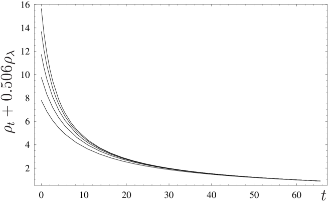
(b)

Figure 3: Evolution of the combination $\rho_{t}(t)+0.506\rho_{\lambda}(t)$ of the Yukawa couplings from the GUT scale ($t=0$) to the electroweak scale ($t=t_{0}$) for $\varkappa^{2}=0$ and for various initial values $h_{t}^{2}(0)$ – Fig. 3a, $\lambda^{2}(0)$ – Fig. 3b.

In analysing the results of numerical calculations, our attention is engaged by a pronounced nonuniformity in the distribution of solutions to the renormalization group equations along the infrared quasi–fixed line. The main reason for this is that, in the regime of strong Yukawa coupling, the solutions in question are attracted not only to the quasi–fixed but also to the infrared fixed (or invariant) line. The latter connects two fixed points. Of these, one is an infrared fixed point of the set of renormalization group equations within the NMSSM ($\rho_{t}=7/18$, $\rho_{\lambda}=0$, $\rho_{1}=0$, $\rho_{2}=0$) B6 , while the other fixed point $(\rho_{\lambda}/\rho_{t}=1)$ corresponds to values of the Yukawa coupling constants in the region $Y_{t},Y_{\lambda}\gg\tilde{\alpha}_{i}$, in which case the gauge coupling constants on the right–hand sides of the renormalization group equations can be disregarded B35 . For the asymptotic behaviour of the infrared fixed line at $\rho_{t},\rho_{\lambda}\gg 1$ we have

$$\rho_{\lambda}=\rho_{t}-\frac{8}{15}-\frac{2}{75}\rho_{1},$$

while in the vicinity of the point $\rho_{t}=7/18$, $\rho_{\lambda}=0$ we have

$$\rho_{\lambda}\sim(\rho_{t}-7/18)^{25/14}.$$

The infrared fixed line is invariant under renormalization group transformations – that is, it is independent of the scale at which the boundary values $Y_{t}(0)$ and $Y_{\lambda}(0)$ are specified and of the boundary values themselves. If the boundary conditions are such that $Y_{t}(0)$ and $Y_{\lambda}(0)$ belong to the fixed line, the evolution of the Yukawa coupling constants proceeds further along this line toward the infrared fixed point of the set of renormalization group equations within the NMSSM. With increasing $t$, all other solutions to the renormalization group equations are attracted to the infrared fixed line and, for $t/(4\pi)\gg 1$, approach the stable infrared fixed point. From the data in Figs. 1 and 2, it follows that, with increasing $Y_{t}(0)$ and $Y_{\lambda}(0)$, all solutions to the renormalization group equations are concentrated in the vicinity of the point of intersection of the infrared fixed and the quasi–fixed line:

$$\rho^{\text{QFP}}_{t}(t_{0})=0.803,\qquad\rho^{\text{QFP}}_{\lambda}(t_{0})=0.224.$$

Hence, this point can be considered as the quasi–fixed point of the set of renormalization group equations within the NMSSM at $\varkappa=0$.

In a more complicated case where all three Yukawa coupling constants in the NMSSM are nonzero, analysis of the set of renormalization group equations presents a much more difficult problem. In particular, invariant (infrared fixed) and Hill surfaces come to the fore instead of the infrared fixed and quasi–fixed lines. For each fixed set of values of the coupling constants $Y_{t}(t_{0})$ and $Y_{\varkappa}(t_{0})$, an upper limit on $Y_{\lambda}(t_{0})$ can be obtained from the requirement that perturbation theory be applicable up to the Grand Unification scale $M_{X}$. A change in the values of the Yukawa coupling constants $h_{t}$ and $\varkappa$ at the electroweak scale leads to a growth or a reduction of the upper limit on $Y_{\lambda}(t_{0})$. The resulting surface in the $(\rho_{t},\rho_{\varkappa},\rho_{\lambda})$ space is shown in Fig. 4. In the regime of strong Yukawa coupling, solutions to the renormalization group equations are concentrated near this surface. In just the same way as in the case of $Y_{\varkappa}=0$, a specific linear combination of $Y_{t}$, $Y_{\lambda}$, and $Y_{\varkappa}$ is virtually independent of the initial conditions for $Y_{i}(0)\to\infty$:

$$\rho_{t}(t_{0})+0.72\rho_{\lambda}(t_{0})+0.33\rho_{\varkappa}(t_{0})=0.98.$$ (6)

The evolution of this combination of Yukawa couplings at various initial values of the Yukawa coupling constants is illustrated in Fig. 5.

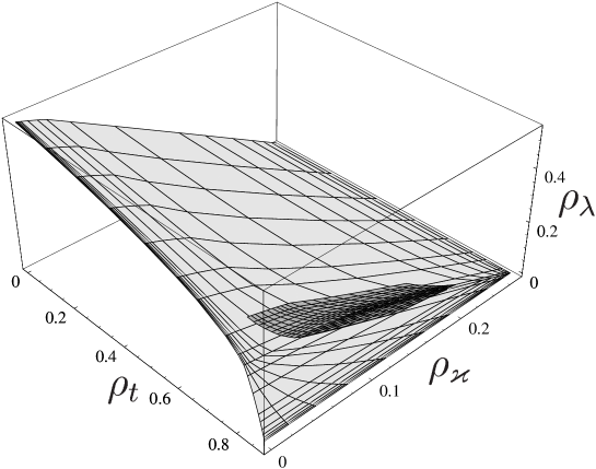
(a)

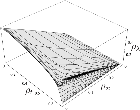
(b)

Figure 4: Quasi–fixed surface in the $(\rho_{t},\rho_{\varkappa},\rho_{\lambda})$ space. The shaded part of the surface represents the region near which the solutions corresponding to the initial values $2\leq h_{t}^{2}(0),\varkappa^{2}(0),\lambda^{2}(0)\leq 10$ – Fig. 4a, $20\leq h_{t}^{2}(0),\varkappa^{2}(0),\lambda^{2}(0)\leq 100$ – Fig. 4b are concentrated.

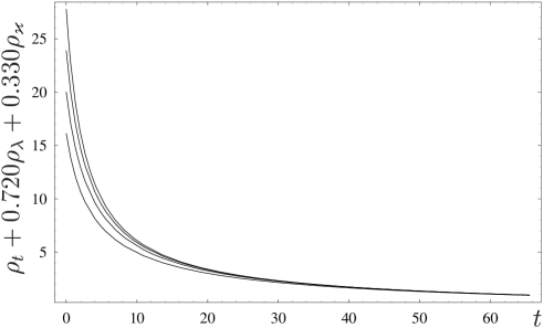
(a)

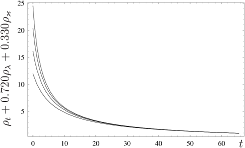
(b)

(c)

Figure 5: Evolution of the combination $\rho_{t}+0.720\rho_{\lambda}+0.3330\rho_{\varkappa}$ of the Yukawa couplings from the GUT scale ($t=0$) to the electroweak scale ($t=t_{0}$) for various initial values $h_{t}^{2}(0)$ – Fig. 5a, $\lambda^{2}(0)$ – Fig. 5b, $\varkappa^{2}(0)$ – Fig. 5c.

On the Hill surface, the region that is depicted in Fig. 4 and near which the solutions in question are grouped shrinks in one direction with increasing initial values of the Yukawa coupling constants, with the result that, at $Y_{t}(0)$, $Y_{\varkappa}(0)$, and $Y_{\lambda}(0)\sim 1$, all solutions are grouped around the line that appears as the result of intersection of the quasi–fixed surface and the infrared fixed surface, which includes the invariant lines lying in the $\rho_{\varkappa}=0$ and $\rho_{\lambda}=0$ planes and connecting the stable infrared point with, respectively, the fixed point $\rho_{\lambda}/\rho_{t}=1$ and the fixed point $\rho_{\varkappa}/\rho_{t}=1$ in the regime of strong Yukawa coupling. In the limit $\rho_{t},\rho_{\lambda},\rho_{\varkappa}\gg 1$, in which case the gauge coupling constants can be disregarded, the fixed points $\rho_{\lambda}/\rho_{t}=1,~{}\rho_{\varkappa}/\rho_{t}=0$ and $\rho_{\varkappa}\rho_{t}=1,~{}\rho_{\lambda}/\rho_{t}=0$ cease to be stable. Instead of them, the stable fixed point $R_{\lambda}=3/4,~{}R_{\varkappa}=3/8$ B35 appears in the $(R_{\lambda},R_{\varkappa})$ plane, where $R_{\lambda}=\rho_{\lambda}/\rho_{t}$ and $R_{\varkappa}=\rho_{\varkappa}/\rho_{t}$. In order to investigate the behaviour of the solutions to the renormalization group equations within the NMSSM, it is necessary to linearise the set of these equations in its vicinity and set $\alpha_{i}=0$. As a result, we obtain

$$\begin{split}R_{\lambda}(t)=&\frac{3}{4}+\left(\frac{1}{2}R_{\lambda 0}+\frac{1}{\sqrt{5}}R_{\varkappa 0}-\frac{3(\sqrt{5}+1)}{8\sqrt{5}}\right)\left(\frac{\rho_{t}(t)}{\rho_{t0}}\right)^{\lambda_{1}}\\ &{}+\left(\frac{1}{2}R_{\lambda 0}-\frac{1}{\sqrt{5}}R_{\varkappa 0}-\frac{3(\sqrt{5}-1)}{8\sqrt{5}}\right)\left(\frac{\rho_{t}(t)}{\rho_{t0}}\right)^{\lambda_{2}},\\ R_{\varkappa}(t)=&\frac{3}{8}+\frac{\sqrt{5}}{2}\left(\frac{1}{2}R_{\lambda 0}+\frac{1}{\sqrt{5}}R_{\varkappa 0}-\frac{3(\sqrt{5}+1)}{8\sqrt{5}}\right)\left(\frac{\rho_{t}(t)}{\rho_{t0}}\right)^{\lambda_{1}}\\ &{}-\frac{\sqrt{5}}{2}\left(\frac{1}{2}R_{\lambda 0}-\frac{1}{\sqrt{5}}R_{\varkappa 0}-\frac{3(\sqrt{5}-1)}{8\sqrt{5}}\right)\left(\frac{\rho_{t}(t)}{\rho_{t0}}\right)^{\lambda_{2}},\\ \end{split}$$ (7)

where $R_{\lambda 0}=R_{\lambda}(0)$, $R_{\varkappa 0}=R_{\varkappa}(0)$, $\rho_{t0}=\rho_{t}(0)$, $\lambda_{1}=\dfrac{3+\sqrt{5}}{9}$, $\lambda_{2}=\dfrac{3-\sqrt{5}}{9}$, and $\rho_{t}(t)=\dfrac{\rho_{t0}}{1+7\rho_{t0}t}$. From (7), it follows that the fixed point $R_{\lambda}=3/4,~{}R_{\varkappa}=3/8$ arises as the result of intersection of two fixed lines in the $(R_{\lambda},R_{\varkappa})$ plane. The solutions are attracted most strongly to the line $\dfrac{1}{2}R_{\lambda}+\dfrac{1}{\sqrt{5}}R_{\varkappa}=\dfrac{3}{8}\left(1+\dfrac{1}{\sqrt{5}}\right)$, since $\lambda_{1}\gg\lambda_{2}$. This line passes through three fixed points in the $(R_{\lambda},R_{\varkappa})$ plane: $(1,0)$, $(3/4,3/8)$, and $(0,1)$. In the regime of strong Yukawa coupling, the fixed line that corresponds, in the $(\rho_{t},\rho_{\varkappa},\rho_{\lambda})$ space, to the line mentioned immediately above is that which lies on the invariant surface containing a stable infrared fixed point. The line of intersection of the Hill and the invariant surface can be obtained by mapping this fixed line into the quasi–fixed surface with the aid of the set of renormalization group equations. For the boundary conditions, one must than use the values $\lambda^{2}(0)$, $\varkappa^{2}(0)$, and $h_{t}^{2}(0)\gg 1$ belonging to the aforementioned fixed line.

In just the same way as infrared fixed lines, the infrared fixed surface is invariant under renormalization group transformations. In the evolution process, solutions to the set of renormalization group equations within the NMSSM are attracted to this surface. If boundary conditions are specified n the fixed surface, the ensuing evolution of the coupling constants proceeds within this surface. To add further details, we not that, near the surface being studied and on it, the solutions are attracted to the invariant line connecting the stable fixed point $(\rho_{\lambda}/\rho_{t}=3/4,~{}\rho_{\varkappa}/\rho_{t}=3/8)$ in the regime of strong Yukawa coupling with the stable infrared fixed point within the NMSSM. In the limit $\rho_{t},\rho_{\varkappa},\rho_{\lambda}\gg 1$, the equation for this line has the form

$$\begin{split}\rho_{\lambda}&=\frac{3}{4}\rho_{t}-\frac{176}{417}+\frac{3}{139}\rho_{2}-\frac{7}{417}\rho_{1},\\ \rho_{\varkappa}&=\frac{3}{8}\rho_{t}-\frac{56}{417}-\frac{18}{139}\rho_{2}-\frac{68}{2085}\rho_{1}.\end{split}$$ (8)

As one approaches the infrared fixed point, the quantities $\rho_{\lambda}$ and $\rho_{\varkappa}$ tend to zero: $\rho_{\lambda}\sim(\rho_{t}-7/18)^{25/14}$ and $\rho_{\varkappa}\sim(\rho_{t}-7/18)^{9/7}$. This line intersects the quasi–fixed surface at the point

$$\rho^{\text{QFP}}_{t}(t_{0})=0.82,\quad\rho^{\text{QFP}}_{\varkappa}(t_{0})=0.087,\quad\rho^{\text{QFP}}_{\lambda}(t_{0})=0.178.$$

Since all solutions are concentrated in the vicinity of this point for $Y_{t}(0),Y_{\lambda}(0)$, $Y_{\varkappa}(0)\to\infty$, it should be considered as a quasi–fixed point for the set of renormalization group equations within the NMSSM. We note, however, that the solutions are attracted to the invariant line (8) and to the quasi–fixed line on the Hill surface. This conclusion can be drawn from the an analysis of the behaviour of the solutions near the fixed point $(R_{\lambda}=3/4,~{}R_{\varkappa}=3/8)$ (see (7)). Once the solutions have approached the invariant line $\dfrac{1}{2}R_{\lambda}+\dfrac{1}{\sqrt{5}}R_{\varkappa}=\dfrac{3}{8}\left(1+\dfrac{1}{\sqrt{5}}\right)$, their evolution is governed by the expression $(\epsilon(t))^{0.085}$, where $\epsilon(t)=\rho_{t}(t)/\rho_{t0}$. This means that the solutions begin to be attracted to the quasi–fixed point and to the invariant line (8) with a sizable strength only when $Y_{i}(0)$ reaches a value of $10^{2}$, at which perturbation theory is obviously inapplicable. Thus, it is not the infrared quasi–fixed point but the quasi–fixed line on the Hill surface (see Fig. 4) that, within the NMSSM, plays a key role in analysing the behaviour of the solutions to the renormalization group equations in the regime of strong Yukawa coupling, where all $Y_{i}(0)$ are much greater than $\tilde{\alpha}_{0}$.

3 Renormalization of the soft SUSY breaking parameters

If the evolution of gauge and Yukawa coupling constants is known, the remaining subset of renormalization group equations within the MNSSM can be treated as a set of linear differential equations for the parameters of a soft breakdown of supersymmetry. For universal boundary conditions, a general solution for the trilinear coupling constants $A_{i}(t)$ and for the masses of scalar fields $m_{i}^{2}(t)$ has the form

$$A_{i}(t)=e_{i}(t)A+f_{i}(t)M_{1/2}\,,$$ (9)

$$m_{i}^{2}(t)=a_{i}(t)m_{0}^{2}+b_{i}(t)M_{1/2}^{2}+c_{i}(t)AM_{1/2}+d_{i}(t)A^{2}\,.$$ (10)

The functions $e_{i}(t)$, $f_{i}(t)$, $a_{i}(t)$, $b_{i}(t)$, $c_{i}(t)$, and $d_{i}(t)$, which determine the evolution of $A_{i}(t)$ and $m_{i}^{2}(t)$, remain unknown, since an analytic solution to the full set of renormalization group equations within the NMSSM is unavailable. These functions greatly depend on the choice of values for the Yukawa coupling constants at the Grand Unification scale $M_{X}$. At the electroweak scale $t=t_{0}$, relations (9) and (10) specify the parameters $A_{i}^{2}(t_{0})$ and $m_{i}^{2}(t_{0})$ of a soft breaking of supersymmetry as functions of their initial values at the Grand Unification scale.

The results of our numerical analysis indicate that, with increasing $Y_{i}(0)$, where $Y_{t}(t)=\dfrac{h_{t}^{2}(t)}{(4\pi)^{2}}$, $Y_{\lambda}(t)=\dfrac{\lambda^{2}(t)}{(4\pi)^{2}}$, and $Y_{\varkappa}(t)=\dfrac{\varkappa^{2}(t)}{(4\pi)^{2}}$, the functions $e_{i}(t_{0})$, $c_{i}(t_{0})$, and $d_{i}(t_{0})$ decrease and tend to zero in the limit $Y_{i}(0)\to\infty$, relations (9) and (10) becoming much simpler in this limit. Instead of the squares of the scalar particle masses, it is convenient to consider their linear combinations

$$\begin{split}\mathfrak{M}_{t}^{2}(t)&=m_{2}^{2}(t)+m_{Q}^{2}(t)+m_{U}^{2}(t),\\ \mathfrak{M}_{\lambda}^{2}(t)&=m_{1}^{2}(t)+m_{2}^{2}(t)+m_{y}^{2}(t),\\ \mathfrak{M}_{\varkappa}^{2}(t)&=3m_{y}^{2}(t)\end{split}$$ (11)

in analysing the set of renormalization group equations. In the case of universal boundary conditions, the solutions to the differential equations for $\mathfrak{M}_{i}^{2}(t)$ can be represented in the same form as the solutions for $m_{i}^{2}(t)$ (see (10)); that is

$$\mathfrak{M}_{i}^{2}(t)=3\tilde{a}_{i}(t)m_{0}^{2}+\tilde{b}_{i}(t)M_{1/2}^{2}+\tilde{c}_{i}(t)AM_{1/2}+\tilde{d}_{i}(t)A^{2}.$$ (12)

Since the homogeneous equations for $A_{i}(t)$ and $\mathfrak{M}_{i}^{2}(t)$ have the same form, the functions $\tilde{a}_{i}(t)$ and $e_{i}(t)$ coincide; in the limit of strong Yukawa coupling, the $m_{0}^{2}$ dependence disappears in the combinations (11) of the scalar particle masses as the solutions to the renormalization group equations for the Yukawa coupling constants approach quasi–fixed points. This behaviour of the solutions implies that $A_{i}(t)$ and $\mathfrak{M}_{i}^{2}(t)$ corresponding to $Y_{i}(0)\gg\tilde{\alpha}_{i}(0)$ also approach quasi–fixed points. As we see in the previous section, two quasi–fixed points of the renormalization group equations within the NMSSM are of greatest interest from the physical point of view. Of these, one corresponds to the boundary conditions $Y_{t}(0)=Y_{\lambda}(0)\gg\tilde{\alpha}_{i}(0)$ and $Y_{\varkappa}(0)=0$ for the Yukawa coupling constants. The fixed points calculated for the parameters of a soft breaking of supersymmetry by using these values of the Yukawa coupling constants are

$$\rho_{A_{t}}^{\text{QFP}}(t_{0}) \approx 1.77, \rho_{\mathfrak{M}^{2}_{t}}^{\text{QFP}}(t_{0}) \approx 6.09,$$ (13)

$$\rho_{A_{\lambda}}^{\text{QFP}}(t_{0}) \approx-0.42,\qquad \rho_{\mathfrak{M}^{2}_{\lambda}}^{\text{QFP}}(t_{0}) \approx-2.28,$$

where $\rho_{A_{i}}(t)=A_{i}(t)/M_{1/2}$ and $\rho_{\mathfrak{M}_{i}^{2}}(t)=\mathfrak{M}_{i}^{2}/M_{1/2}^{2}$. Since the coupling constant $\varkappa$ for the self–interaction of neutral scalar fields is small in the case being considered, $A_{\varkappa}(t)$ and $\mathfrak{M}_{\varkappa}^{2}(t)$ do not approach the quasi–fixed point. Nonetheless, the spectrum of SUSY particles is virtually independent of the trilinear coupling constant $A_{\varkappa}$ since $\varkappa\to 0$.

In just the same way, one can determine the position of the other quasi–fixed point for $A_{i}(t)$ and $\mathfrak{M}_{i}^{2}(t)$, that which corresponds to $R_{\lambda 0}=3/4,~{}R_{\varkappa 0}=3/8$. The results are

$$\rho_{A_{t}}^{\text{QFP}}(t_{0}) \approx 1.73, \rho_{A_{\lambda}}^{\text{QFP}}(t_{0}) \approx-0.43, \rho_{A_{\varkappa}}^{\text{QFP}}(t_{0}) \approx 0.033,$$ (14)

$$\rho_{\mathfrak{M}^{2}_{t}}^{\text{QFP}}(t_{0}) \approx 6.02,\quad \rho_{\mathfrak{M}^{2}_{\lambda}}^{\text{QFP}}(t_{0}) \approx-2.34,\quad \rho_{\mathfrak{M}^{2}_{\varkappa}}^{\text{QFP}}(t_{0}) \approx 0.29,$$

where $R_{\lambda 0}=Y_{\lambda}(0)/Y_{t}(0)$ and $R_{\varkappa 0}=Y_{\varkappa}(0)/Y_{t}(0)$. It should be noted that, in the vicinities of quasi–fixed points, we have $\rho_{\mathfrak{M}^{2}_{\lambda}}^{\text{QFP}}(t_{0})<0$. Negative values of $\mathfrak{M}_{\lambda}^{2}(t_{0})$ lead to a negative value of the parameter $m_{2}^{2}(t_{0})$ in the potential of interaction of Higgs fields. In other words, an elegant mechanism that is responsible for a radiative violation of $SU(2)\otimes U(1)$ symmetry and which does not require introducing tachyons in the spectrum of the theory from the outset survives in the regime of strong Yukawa coupling within the NMSSM. This mechanism of gauge symmetry breaking was first discussed in C30 by considering the example of the minimal SUSY model.

By using the fact that $\mathfrak{M}_{i}^{2}(t)$ as determined for the case of universal boundary conditions is virtually independent of $m_{0}^{2}$, we can predict $a_{i}(t_{0})$ values near the quasi–fixed points (see NTC ). The results are

$$\begin{split}1)~{}&R_{\lambda 0}=1,~{}R_{\varkappa 0}=0,\\ &a_{y}(t_{0})=a_{u}(t_{0})=\frac{1}{7},~{}a_{1}(t_{0})=a_{q}(t_{0})=\frac{4}{7},~{}a_{2}(t_{0})=-\frac{5}{7}\,;\\ 2)~{}&R_{\lambda 0}=3/4,~{}R_{\varkappa 0}=3/8,\\ &a_{y}(t_{0})=0,~{}a_{1}(t_{0})=-a_{2}(t_{0})=\frac{2}{3},~{}a_{q}(t_{0})=\frac{5}{9},~{}a_{u}(t_{0})=\frac{1}{9}\,.\end{split}$$ (15)

To do this, it was necessary to consider specific combinations of the scalar particle masses, such as $m_{U}^{2}-2m_{Q}^{2}$, $m_{Q}^{2}+m_{U}^{2}-m_{2}^{2}+m_{1}^{2}$, and $m_{y}^{2}-2m_{1}^{2}$ (at $\varkappa=0$), that are not renormalized by Yukawa interactions. As a result, the dependence of the above combinations of the scalar particle masses on $m_{0}^{2}$ at the electroweak scale is identical to that at the Grand Unification scale. The predictions in (15) agree fairly well with the results of numerical calculations.

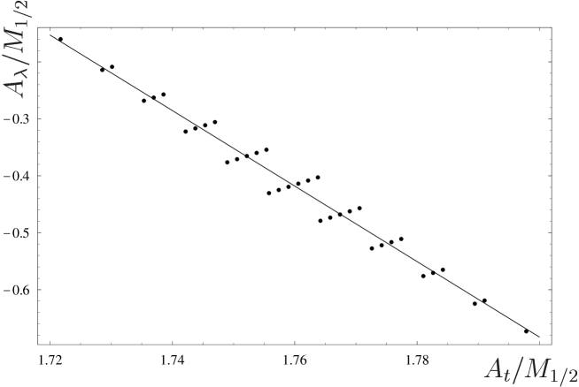
Figure 6: The values of the trilinear couplings $A_{t}$ and $A_{\lambda}$ at the electroweak scale corresponding to the initial values uniformly distributed in the $(A_{t},A_{\lambda})$ plane, calculated at $\varkappa^{2}=0$ and $h_{t}^{2}(0)=\lambda^{2}(0)=20$. The straight line is a fit of the values $(A_{t}(t_{0}),A_{\lambda}(t_{0}))$.

Figure 7: The values of the combinations of masses $\mathfrak{M}_{t}^{2}$ and $\mathfrak{M}_{\lambda}^{2}$ at the electroweak scale corresponding to the initial values uniformly distributed in the $(\mathfrak{M}_{t}^{2}/M_{1/2}^{2},\mathfrak{M}_{\lambda}^{2}/M_{1/2}^{2})$ plane, calculated at $\varkappa^{2}=0$, $h_{t}^{2}(0)=\lambda^{2}(0)=20$, and $A_{t}(0)=A_{\lambda}(0)=0$. The straight line is a fit of the values $(\mathfrak{M}_{t}^{2}(t_{0}),\mathfrak{M}_{\lambda}^{2}(t_{0}))$.

Let us now consider the case of nonuniversal boundary conditions for the soft SUSY breaking parameters. The results of our numerical analysis, which are illustrated in Figs. 6 and 7, indicate that, in the vicinity of the infrared fixed point at $Y_{\varkappa}=0$, solutions to the renormalization group equations at the electroweak scale are concentrated near some straight lines for the case where the simulation was performed by using boundary conditions uniformly distributed in the $(A_{t},A_{\lambda})$ and the $(\mathfrak{M}_{t}^{2},\mathfrak{M}_{\lambda}^{2})$ plane. The strength with which these solutions are attracted to them grows with increasing $Y_{i}(0)$. The equations for the lines being considered can be obtained by fitting the numerical results displayed in Figs. 6 and 7. This yields

$$\begin{gathered}A_{t}+0.147A_{\lambda}=1.70M_{1/2},\\ \mathfrak{M}^{2}_{t}+0.147\mathfrak{M}^{2}_{\lambda}=5.76M_{1/2}^{2}.\end{gathered}$$ (16)

For $Y_{\varkappa}(0)\gg\tilde{\alpha}_{0}$ solutions to the renormalization group equations are grouped near planes in the space of the parameters of a soft breaking of supersymmetry $(A_{t},A_{\lambda},A_{\varkappa})$ and $(\mathfrak{M}_{t}^{2},\mathfrak{M}_{\lambda}^{2},\mathfrak{M}_{\varkappa}^{2})$ (see Figs. 8-10):

$$\begin{gathered}A_{t}+0.128A_{\lambda}+0.022A_{\varkappa}=1.68M_{1/2},\\ \mathfrak{M}^{2}_{t}+0.128\mathfrak{M}^{2}_{\lambda}+0.022\mathfrak{M}^{2}_{\varkappa}=5.77M_{1/2}^{2}.\end{gathered}$$ (17)

It can be seen from Figs. 8 and 9 that, as the values of the Yukawa coupling constants at the Grand Unification scale are increased, the areas of the surfaces near which the solutions $A_{i}(t)$ and $\mathfrak{M}_{i}^{2}(t)$ are concentrated shrink in one of the directions, with the result that, at $Y_{i}(0)\sim 1$, the solutions to the renormalization group equations are attracted to one of the straight lines belonging to these surfaces.

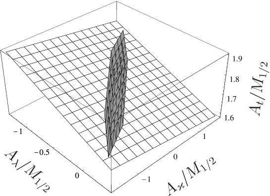
(a)

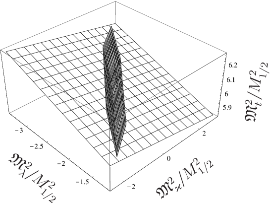
(b)

Figure 8: Planes in the parameter spaces $(A_{t}/M_{1/2},A_{\lambda}/M_{1/2},A_{\varkappa}/M_{1/2})$ – Fig. 8a, and $(\mathfrak{M}_{t}^{2}/M_{1/2}^{2},\mathfrak{M}_{\lambda}^{2}/M_{1/2}^{2},\mathfrak{M}_{\varkappa}^{2}/M_{1/2}^{2})$ – Fig. 8b. The shaded parts of the planes correspond to the regions near which the solutions at $h_{t}^{2}(0)=16$, $\lambda^{2}(0)=12$, and $\varkappa^{2}(0)=6$ are concentrated. The initial values $A_{i}(0)$ and $\mathfrak{M}_{i}^{2}(0)$ vary in the ranges $-M_{1/2}\leq A\leq M_{1/2}$ and $0\leq\mathfrak{M}_{i}^{2}(0)\leq 3M_{1/2}^{2}$, respectively.

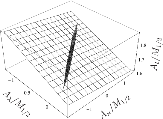
(a)

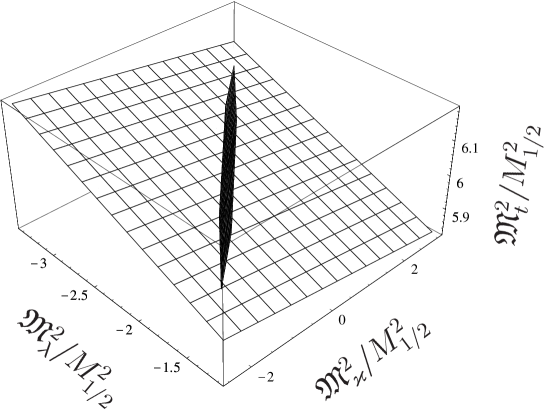
(b)

Figure 9: Planes in the parameter spaces $(A_{t}/M_{1/2},A_{\lambda}/M_{1/2},A_{\varkappa}/M_{1/2})$ – Fig. 9a, and $(\mathfrak{M}_{t}^{2}/M_{1/2}^{2},\mathfrak{M}_{\lambda}^{2}/M_{1/2}^{2},\mathfrak{M}_{\varkappa}^{2}/M_{1/2}^{2})$ – Fig. 9b. The shaded parts of the planes correspond to the regions near which the solutions at $h_{t}^{2}(0)=32$, $\lambda^{2}(0)=24$, and $\varkappa^{2}(0)=12$ are concentrated. The initial values $A_{i}(0)$ and $\mathfrak{M}_{i}^{2}(0)$ vary in the ranges $-M_{1/2}\leq A\leq M_{1/2}$ and $0\leq\mathfrak{M}_{i}^{2}(0)\leq 3M_{1/2}^{2}$, respectively.

The numerical calculations also showed that, with increasing $Y_{i}(0)$, only in the regime of infrared quasi–fixed points (that is, at $R_{\lambda 0}=1,~{}R_{\varkappa 0}=0$ or at $R_{\lambda 0}=3/4,~{}R_{\varkappa 0}=3/8$) $e_{i}(t_{0})$ and $\tilde{a}_{i}(t_{0})$ decrease quite fast, in proportion to $1/Y_{i}(0)$. Otherwise, the dependence on $A$ and $m_{0}^{2}$ disappears much more slowly with increasing values of the Yukawa coupling constants at the Grand Unification scale – specifically, in proportion to $(Y_{i}(0))^{-\delta}$, where $\delta<1$ (for example, $\delta=0.35-0.40$ at $\varkappa=0$). In the case of nonuniversal boundary conditions, only when solutions to the renormalization group equations approach quasi–fixed points are these solutions attracted to the fixed lines and surfaces in the space of the parameters of a soft breaking of supersymmetry, and in the limit $Y_{i}(0)\to\infty$, the parameters $A_{i}(t)$ and $\mathfrak{M}_{i}^{2}(t)$ cease to be dependent on the boundary conditions.

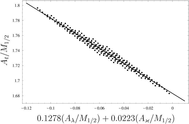
(a)

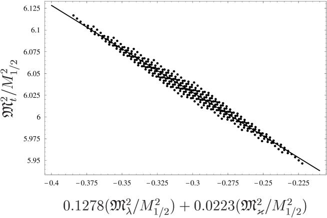
(b)

Figure 10: Set of points in planes $(0.0223(A_{\varkappa}/M_{1/2})+0.1278(A_{\lambda}/M_{1/2}),~{}A_{t}/M_{1/2})$ – Fig. 10a, and $(0.0223(\mathfrak{M}^{2}_{\varkappa}/M_{1/2}^{2})+0.1278(\mathfrak{M}^{2}_{\lambda}/M_{1/2}^{2}),~{}\mathfrak{M}^{2}_{t}/M^{2}_{1/2})$ – Fig. 10b, corresponding to the values of parameters of soft SUSY breaking for $h_{t}^{2}(0)=32$, $\lambda^{2}(0)=24$, $\varkappa^{2}(0)=12$, and for a uniform distribution of the boundary conditions in the parameter spaces $(A_{t},A_{\lambda},A_{\varkappa})$ and $(\mathfrak{M}^{2}_{t},\mathfrak{M}^{2}_{\lambda},\mathfrak{M}^{2}_{\varkappa})$. The initial values $A_{i}(0)$ and $\mathfrak{M}_{i}^{2}(0)$ vary in the ranges $-M_{1/2}\leq A\leq M_{1/2}$ and $0\leq\mathfrak{M}_{i}^{2}(0)\leq 3M_{1/2}^{2}$, respectively. The straight lines in Figs. 10a and 10b correspond to the planes in Figs. 9a and 9b, respectively.

For the solutions of the renormalization group equations for the soft SUSY breaking parameters near the electroweak scale in the strong Yukawa coupling regime one can construct an expansion in powers of the small parameter $\epsilon_{t}(t)=Y_{t}(t)/Y_{t}(0)$:

$$\binom{A_{i}(t)}{\mathfrak{M}^{2}_{i}(t)}=\sum_{k}u_{ik}v_{ik}(t)\binom{\alpha_{k}}{\beta_{k}}(\epsilon_{t}(t))^{\lambda_{k}}+\dots,$$ (18)

where $\alpha_{i}$ and $\beta_{i}$ are constants of integration that can be expressed in terms of $A_{i}(0)$ and $\mathfrak{M}^{2}_{i}(0)$. The functions $v_{ij}(t)$ are weakly dependent on the Yukawa coupling constants at the scale $M_{X}$, and $v_{ij}(0)=1$. They appear upon renormalizing the parameters of a soft breaking of supersymmetry from $q\sim 10^{12}-10^{13}\text{~{}GeV}$ to $q\sim m_{t}$. In equations (18), we have omitted terms proportional to $M_{1/2}$, $M_{1/2}^{2}$, $A_{i}(0)M_{1/2}$, and $A_{i}(0)A_{j}(0)$.

At $\varkappa=0$, we have two eigenvalues and two corresponding eigenvectors:

$$\lambda=\begin{pmatrix}1\\ 3/7\end{pmatrix},\qquad u=\begin{pmatrix}1&1\\ 1&-3\end{pmatrix},$$

whose components specify $(A_{t},A_{\lambda})$ and $(\mathfrak{M}_{t}^{2},\mathfrak{M}_{\lambda}^{2})$. With increasing $Y_{t}(0)\simeq Y_{\lambda}(0)$, the dependence on $\alpha_{0}$ and $\beta_{0}$ becomes weaker and the solutions at $t=t_{0}$ are concentrated near the straight lines $(A_{t}(\alpha_{1}),A_{\lambda}(\alpha_{1}))$ and $(\mathfrak{M}_{t}^{2}(\beta_{1}),\mathfrak{M}_{\lambda}^{2}(\beta_{1}))$. In order to obtain the equations for these straight lines, it is necessary to set $A_{\lambda}(0)=-3A_{t}(0)$ and $\mathfrak{M}_{\lambda}^{2}(0)=-3\mathfrak{M}_{t}^{2}(0)$ at the Grand Unification scale. At the electroweak scale, there then arise a relation between $A_{t}(t_{0})$ and $A_{\lambda}(t_{0})$ and a relation between $\mathfrak{M}_{t}^{2}(t_{0})$ and $\mathfrak{M}_{\lambda}^{2}(t_{0})$:

$$\begin{gathered}A_{t}+0.137A_{\lambda}=1.70M_{1/2},\\ \mathfrak{M}^{2}_{t}+0.137\mathfrak{M}^{2}_{\lambda}=5.76M^{2}_{1/2}.\end{gathered}$$ (19)

These relations agree well with the equations deduced for the straight lines at $Y_{i}(0)\sim 1$ by fitting the results of the numerical calculations (16).

When the Yukawa coupling constant $\varkappa$ is nonzero, we have three eigenvalues and three corresponding eigenvectors:

$$\lambda=\begin{pmatrix}1\\ \frac{3+\sqrt{5}}{9}\\ \frac{3-\sqrt{5}}{9}\end{pmatrix},\qquad u=\begin{pmatrix}1&-\frac{1+\sqrt{5}}{24}&\frac{\sqrt{5}-1}{24}\\ 1&\frac{\sqrt{5}}{6}&-\frac{\sqrt{5}}{6}\\ 1&1&1\end{pmatrix},$$

whose components specify $(A_{t},A_{\lambda},A_{\varkappa})$ and $(\mathfrak{M}_{t}^{2},\mathfrak{M}_{\lambda}^{2},\mathfrak{M}_{\varkappa}^{2})$. An increase in $Y_{\lambda}(0)\simeq 2Y_{\varkappa}(0)\simeq\dfrac{3}{4}Y_{t}(0)$ leads to the following: first, the dependence of $A_{i}(t)$ and $\mathfrak{M}_{i}^{2}(t)$ on $\alpha_{0}$ and $\beta_{0}$ disappears, which leads to the emergence of planes in the space spanned by the parameters of a soft breaking of supersymmetry:

$$\begin{gathered}A_{t}+0.103A_{\lambda}+0.0124A_{\varkappa}=1.69M_{1/2},\\ \mathfrak{M}^{2}_{t}+0.103\mathfrak{M}^{2}_{\lambda}+0.0124\mathfrak{M}^{2}_{\varkappa}=5.78M^{2}_{1/2}.\end{gathered}$$ (20)

After that, the dependence on $\alpha_{1}$ and $\beta_{1}$ becomes weaker at $Y_{i}(0)\sim 1$. This means that, with increasing initial values of the Yukawa coupling constants, solutions to the renormalization group equations are grouped near some straight lines and we can indeed see precisely this pattern in Figs. 8-10. All equations presented here for the straight lines and planes in the $\mathfrak{M}_{i}^{2}$ space were obtained at $A_{i}(0)=0$.

From relations (19) and (20), it follows that $A_{t}(t_{0})$ and $\mathfrak{M}_{t}^{2}(t_{0})$ are virtually independent of the initial conditions; that is, the straight lines and planes are orthogonal to the $A_{t}$ and $\mathfrak{M}_{t}^{2}$ axes. On the other hand, the $A_{\varkappa}(t_{0})$ and $\mathfrak{M}_{\varkappa}^{2}(t_{0})$ values that correspond to the Yukawa self–interaction constant $Y_{\varkappa}$ for the neutral fields are fully determined by the boundary conditions for the parameters of a soft breaking of supersymmetry. For this reason, the planes in the $(A_{t},A_{\lambda},A_{\varkappa})$ and $(\mathfrak{M}_{t}^{2},\mathfrak{M}_{\lambda}^{2},\mathfrak{M}_{\varkappa}^{2})$ spaces are virtually parallel to the $A_{\varkappa}$ and $\mathfrak{M}_{\varkappa}^{2}$ axes.

4 Conclusions

In the strong Yukawa coupling regime in the NMSSM, solutions to the renormalization group equations for $Y_{i}(t)$ are attracted to quasi–fixed lines and surfaces in the space of Yukawa coupling constants and specific combinations of $\rho_{i}(t)$ are virtually independent of their initial values at the Grand Unification scale. For $Y_{i}(0)\to\infty$, all solutions to the renormalization group equations are concentrated near quasi–fixed points. These points emerge as the result of intersection of Hill lines or surfaces with the invariant line that connects the stable fixed point for $Y_{i}\gg\tilde{\alpha}_{i}$ with the stable infrared fixed point. For the renormalization group equations within the NMSSM, we have listed all the most important invariant lines and surfaces and studied their asymptotic behaviour for $Y_{i}\gg\tilde{\alpha}_{i}$ and in the vicinity of the infrared fixed point.

With increasing $Y_{i}(0)$, the solutions in question approach quasi–fixed points quite slowly; that is, the deviation is proportional to $(\epsilon_{t}(t))^{\delta}$, where $\epsilon_{t}(t)=Y_{t}(t)/Y_{t}(0)$ and $\delta$ is calculated by analysing the set of the renormalization group equations in the regime of strong Yukawa coupling. As a rule, $\delta$ is positive and much less than unity. By way of example, we indicate that, in the case where all three Yukawa coupling constants differ from zero, $\delta\approx 0.085$. Of greatest importance in analysing the behaviour of solutions to the renormalization group equations within the NMSSM at $Y_{t}(0),Y_{\lambda}(0),Y_{\varkappa}(0)\sim 1$ is therefore not the infrared quasi–fixed point but the line lying on the Hill surface and emerging as the intersection of the Hill and invariant surface. This line can be obtained by mapping the fixed points $(1,0)$, $(3/4,3/8)$, and $(0,1)$ in the $(R_{\lambda},R_{\varkappa})$ plane for $Y_{i}\gg\tilde{\alpha}_{i}$ into the quasi–fixed surface by means of renormalization group equations.

While $Y_{i}(t)$ approach quasi–fixed points, the corresponding solutions for the trilinear coupling constants $A_{i}(t)$ characterising scalar fields and for the combinations $\mathfrak{M}_{i}^{2}(t)$ of the scalar particle masses (see (11)) cease to be dependent on their initial values at the scale $M_{X}$ and, in the limit $Y_{i}(0)\to\infty$, also approach the fixed points in the space spanned by the parameters of a soft breaking of supersymmetry. Since the set of differential equations for $A_{i}(t)$ and $m_{i}^{2}(t)$ is linear, the $A$, $M_{1/2}$, and $m_{0}^{2}$ dependence of the parameters of a soft breaking of supersymmetry at the electroweak scale can be explicitly obtained for universal boundary conditions. It turns out that, near the quasi–fixed points, all $A_{i}(t)$ and all $\mathfrak{M}_{i}^{2}(t)$ are proportional to $M_{1/2}$ and $M_{1/2}^{2}$, respectively. Thus, we have shown that, in the parameter space region considered here, the solutions to the renormalization group equations for the trilinear coupling constants and for some combinations of the scalar particle masses are focused in a narrow interval within the infrared region. Since the neutral scalar field $Y$ is not renormalized by gauge interactions, $A_{\varkappa}(t)$ and $\mathfrak{M}_{\varkappa}^{2}(t)$ are concentrated near zero; therefore they are still dependent on the initial conditions. The parameters $A_{t}(t_{0})$ and $\mathfrak{M}_{t}^{2}(t_{0})$ show the weakest dependence on $A$ and $m_{0}^{2}$ because these parameters are renormalized by strong interactions. By considering that the quantities $\mathfrak{M}_{i}^{2}(t_{0})$ are virtually independent of the boundary conditions, we have calculated, near the quasi–fixed points, the values of the scalar particle masses at the electroweak scale.

In the general case of nonuniversal boundary conditions, the solutions to the renormalization group equations within the NMSSM for $A_{i}(t)$ and $\mathfrak{M}_{i}^{2}(t)$ are grouped near some straight lines and planes in the space spanned by the parameters of a soft breaking of supersymmetry. Moving along these lines and surfaces as $Y_{i}(0)$ is increased, the trilinear coupling constants and the above combinations of the scalar particle masses approach quasi–fixed points. However, the dependence of these couplings on $A_{i}(0)$ and $\mathfrak{M}_{i}^{2}(0)$ dies out quite slowly, in proportion to $(\epsilon_{t}(t))^{\lambda}$, where $\lambda$ is a small positive number; as a rule, $\lambda\ll 1$. For example, $\lambda=3/7$ at $Y_{\varkappa}=0$ and $\lambda\approx 0.0085$ at $Y_{\varkappa}\neq 0$. The above is invalid only for the solutions $A_{i}(t)$ and $\mathfrak{M}_{i}^{2}(t)$ that correspond to universal boundary conditions for the parameters of a soft breaking of supersymmetry and to the initial values of $R_{\lambda 0}=1,~{}R_{\varkappa 0}=0$ and $R_{\lambda 0}=3/4,~{}R_{\varkappa 0}=3/8$ for the Yukawa coupling constants at the Grand Unification scale. They correspond to quasi–fixed points of the renormalization group equations for $Y_{i}(t)$. As the Yukawa coupling constants are increased, such solutions are attracted to infrared quasi–fixed points in proportion to $\epsilon_{t}(t)$.

Straight lines in the $(A_{t},A_{\lambda},A_{\varkappa})$ and $(\mathfrak{M}_{t}^{2},\mathfrak{M}_{\lambda}^{2},\mathfrak{M}_{\varkappa}^{2})$ spaces play a key role in the analysis of the behaviour of solutions for $A_{i}(t)$ and $\mathfrak{M}_{i}^{2}(t)$ in the case where $Y_{t}(0),Y_{\lambda}(0),Y_{\varkappa}(0)\sim 1$. In the space spanned by the parameters of a soft breaking of supersymmetry, these straight lines lie in the planes near which $A_{i}(t)$ and $\mathfrak{M}_{i}^{2}(t)$ are grouped in the regime of strong Yukawa coupling at the electroweak scale. The straight lines and planes that were obtained by fitting the results of numerical calculations are nearly orthogonal to the $A_{t}$ and $\mathfrak{M}_{t}^{2}$ axes. This is because the constants $A_{t}(t_{0})$ and $\mathfrak{M}_{t}^{2}(t_{0})$ are virtually independent of the initial conditions at the scale $M_{X}$. On the other hand, the parameters $A_{\varkappa}(t_{0})$ and $\mathfrak{M}_{\varkappa}^{2}(t_{0})$ are determined, to a considerable extent, by the boundary conditions at the scale $M_{X}$. At $R_{\lambda 0}=3/4$ and $R_{\varkappa 0}=3/8$, the planes in the $(A_{t},A_{\lambda},A_{\varkappa})$ and $(\mathfrak{M}_{t}^{2},\mathfrak{M}_{\lambda}^{2},\mathfrak{M}_{\varkappa}^{2})$ spaces are therefore parallel to the $A_{\varkappa}$ and $\mathfrak{M}_{\varkappa}^{2}$ axes.

*Multiple Point Model and Phase Transition Couplings in the Two-Loop Approximation of Dual Scalar Electrodynamics L.V. Laperashvili^a, D.A. Ryzhikh^a and H.B. Nielsen^b

The simplest effective dynamics describing the confinement mechanism in the pure gauge lattice U(1) theory is the dual Abelian Higgs model of scalar monopoles [1-3].

In the previous papers [4-6] the calculations of the U(1) phase transition (critical) coupling constant were connected with the existence of artifact monopoles in the lattice gauge theory and also in the Wilson loop action model 6 . In Ref.6 we (L.V.L. and H.B.N.) have put forward the speculations of Refs.[4,5] suggesting that the modifications of the form of the lattice action might not change too much the phase transition value of the effective continuum coupling constant. In 6 the Wilson loop action was considered in the approximation of circular loops of radii $R\geq a$. It was shown that the phase transition coupling constant is indeed approximately independent of the regularization method: ${\alpha}_{crit}\approx{0.204}$, in correspondence with the Monte Carlo simulation result on lattice 7 : ${\alpha}_{crit}\approx{0.20\pm 0.015}$.

But in Refs.[2,3] instead of using the lattice or Wilson loop cut–off we have considered the Higgs Monopole Model (HMM) approximating the lattice artifact monopoles as fundamental pointlike particles described by the Higgs scalar field.

5 The Coleman-Weinberg effective potential for the Higgs monopole model

The dual Abelian Higgs model of scalar monopoles (shortly HMM), describing the dynamics of confinement in lattice theories, was first suggested in Ref.1 , and considers the following Lagrangian:

$$L=-\frac{1}{4g^{2}}F_{\mu\nu}^{2}(B)+\frac{1}{2}|(\partial_{\mu}-iB_{\mu})\Phi|^{2}-U(\Phi),\quad{\mbox{where}}\quad U(\Phi)=\frac{1}{2}\mu^{2}{|\Phi|}^{2}+\frac{\lambda}{4}{|\Phi|}^{4}$$ (21)

is the Higgs potential of scalar monopoles with magnetic charge $g$, and $B_{\mu}$ is the dual gauge (photon) field interacting with the scalar monopole field $\Phi$. In this model $\lambda$ is the self–interaction constant of scalar fields, and the mass parameter $\mu^{2}$ is negative. In Eq.(21) the complex scalar field $\Phi$ contains the Higgs ($\phi$) and Goldstone ($\chi$) boson fields:

$$\Phi=\phi+i\chi.$$ (22)

The effective potential in the Higgs Scalar ElectroDynamics (HSED) was first calculated by Coleman and Weinberg 9 in the one–loop approximation. The general method of its calculation is given in the review 10 . Using this method, we can construct the effective potential for HMM. In this case the total field system of the gauge ($B_{\mu}$) and magnetically charged ($\Phi$) fields is described by the partition function which has the following form in Euclidean space:

$$Z=\int[DB][D\Phi][D\Phi^{+}]\,e^{-S},$$ (23)

where the action $S=\int d^{4}xL(x)+S_{gf}$ contains the Lagrangian (21) written in Euclidean space and gauge fixing action $S_{gf}$. Let us consider now a shift: $\Phi(x)=\Phi_{b}+{\hat{\Phi}}(x)$ with $\Phi_{b}$ as a background field and calculate the following expression for the partition function in the one-loop approximation:

$$Z=\int[DB][D\hat{\Phi}][D{\hat{\Phi}}^{+}]\exp\{-S(B,\Phi_{b})-\int d^{4}x[\frac{\delta S(\Phi)}{\delta\Phi(x)}|_{\Phi=\Phi_{b}}{\hat{\Phi}}(x)+h.c.]\}\\$$

$$=\exp\{-F(\Phi_{b},g^{2},\mu^{2},\lambda)\}.$$ (24)

Using the representation (22), we obtain the effective potential:

$$V_{eff}=F(\phi_{b},g^{2},\mu^{2},\lambda)$$ (25)

given by the function $F$ of Eq.(24) for the constant background field $\Phi_{b}=\phi_{b}=\mbox{const}$. In this case the one–loop effective potential for monopoles coincides with the expression of the effective potential calculated by the authors of Ref.9 for scalar electrodynamics and extended to the massive theory (see review 10 ). As it was shown in Ref.9 , the effective potential can be improved by consideration of the renormalization group equation (RGE).

6 Renormalization group equations in the Higgs monopole model

The RGE for the effective potential means that the potential cannot depend on a change in the arbitrary parameter — renormalization scale $M$:

$$\frac{dV_{eff}}{dM}=0.$$ (26)

The effects of changing it are absorbed into changes in the coupling constants, masses and fields, giving so–called running quantities.

Considering the RG improvement of the effective potential [8,9] and choosing the evolution variable as

$$t=\log(\phi^{2}/M^{2}),$$ (27)

we have the following RGE for the improved $V_{eff}(\phi^{2})$ with $\phi^{2}\equiv\phi^{2}_{b}$ 11 :

$$(M^{2}\frac{\partial}{\partial M^{2}}+\beta_{\lambda}\frac{\partial}{\partial\lambda}+\beta_{g}\frac{\partial}{\partial g^{2}}+\beta_{(\mu^{2})}\mu^{2}\frac{\partial}{\partial\mu^{2}}-\gamma\phi^{2}\frac{\partial}{\partial\phi^{2}})V_{eff}(\phi^{2})=0,$$ (28)

where $\gamma$ is the anomalous dimension and $\beta_{(\mu^{2})}$, $\beta_{\lambda}$ and $\beta_{g}$ are the RG $\beta$–functions for mass, scalar and gauge couplings, respectively. RGE (28) leads to the following form of the improved effective potential 9 :

$$V_{eff}=\frac{1}{2}\mu^{2}_{run}(t)G^{2}(t)\phi^{2}+\frac{1}{4}\lambda_{run}(t)G^{4}(t)\phi^{4}.$$ (29)

In our case:

$$G(t)=\exp[-\frac{1}{2}\int_{0}^{t}dt^{\prime}\,\gamma\left(g_{run}(t^{\prime}),\lambda_{run}(t^{\prime})\right)].$$ (30)

A set of ordinary differential equations (RGE) corresponds to Eq.(28):

$$\frac{d\lambda_{run}}{dt}=\beta_{\lambda}\left(g_{run}(t),\,\lambda_{run}(t)\right),$$ (31)

$$\frac{d\mu^{2}_{run}}{dt}=\mu^{2}_{run}(t)\beta_{(\mu^{2})}\left(g_{run}(t),\,\lambda_{run}(t)\right),$$ (32)

$$\frac{dg^{2}_{run}}{dt}=\beta_{g}\left(g_{run}(t),\,\lambda_{run}(t)\right).$$ (33)

So far as the mathematical structure of HMM is equivalent to HSED, we can use all results of the scalar electrodynamics in our calculations, replacing the electric charge $e$ and photon field $A_{\mu}$ by magnetic charge $g$ and dual gauge field $B_{\mu}$.

The one–loop results for $\beta_{\lambda}^{(1)}$, $\beta_{\mu^{2}}^{(1)}$ and $\gamma$ are given in Ref.9 for scalar field with electric charge $e$, but it is easy to rewrite them for monopoles with charge $g=g_{run}$:

$$\gamma^{(1)}=-\frac{3g_{run}^{2}}{16\pi^{2}},$$ (34)

$$\frac{d\lambda_{run}}{dt}\approx\beta_{\lambda}^{(1)}=\frac{1}{16\pi^{2}}(3g^{4}_{run}+10\lambda^{2}_{run}-6\lambda_{run}g^{2}_{run}),$$ (35)

$$\frac{d\mu^{2}_{run}}{dt}\approx\beta_{(\mu^{2})}^{(1)}=\frac{\mu^{2}_{run}}{16\pi^{2}}(4\lambda_{run}-3g^{2}_{run}),$$ (36)

$$\frac{dg^{2}_{run}}{dt}\approx\beta_{g}^{(1)}=\frac{g^{4}_{run}}{48\pi^{2}}.$$ (37)

The RG $\beta$–functions for different renormalizable gauge theories with semisimple group have been calculated in the two–loop approximation and even beyond. But in this paper we made use the results of Refs.12 and 13 for calculation of $\beta$–functions and anomalous dimension in the two–loop approximation, applied to the HMM with scalar monopole fields. The higher approximations essentially depend on the renormalization scheme. Thus, on the level of two–loop approximation we have for all $\beta$–functions:

$$\beta=\beta^{(1)}+\beta^{(2)},$$ (38)

where

$$\beta_{\lambda}^{(2)}=\frac{1}{(16\pi^{2})^{2}}(-25\lambda^{3}+\frac{15}{2}g^{2}{\lambda}^{2}-\frac{229}{12}g^{4}\lambda-\frac{59}{6}g^{6}),$$ (39)

and

$$\beta_{(\mu^{2})}^{(2)}=\frac{1}{(16\pi^{2})^{2}}(\frac{31}{12}g^{4}+3\lambda^{2}).$$ (40)

The gauge coupling $\beta_{g}^{(2)}$–function is given by Ref.12 :

$$\beta_{g}^{(2)}=\frac{g^{6}}{(16\pi^{2})^{2}}.$$ (41)

Anomalous dimension follows from calculations made in Ref.13 :

$$\gamma^{(2)}=\frac{1}{(16\pi^{2})^{2}}\frac{31}{12}g^{4}.$$ (42)

In Eqs.(38)–(42) and below, for simplicity, we have used the following notations: $\lambda\equiv\lambda_{run}$, $g\equiv g_{run}$ and $\mu\equiv\mu_{run}$.

7 The phase diagram in the Higgs monopole model

Now we want to apply the effective potential calculation as a technique for the getting phase diagram information for the condensation of monopoles in HMM. If the first local minimum occurs at $\phi=0$ and $V_{eff}(0)=0$, it corresponds to the Coulomb–like phase. In the case when the effective potential has the second local minimum at $\phi=\phi_{min}\neq 0\,$ with $\,V_{eff}^{min}(\phi_{min}^{2})<0$, we have the confinement phase. The phase transition between the Coulomb–like and confinement phases is given by the condition when the first local minimum at $\phi=0$ is degenerate with the second minimum at $\phi=\phi_{0}$. These degenerate minima are shown in Fig.1 by the curve 1. They correspond to the different vacua arising in this model. And the dashed curve 2 describes the appearance of two minima corresponding to the confinement phases.

The conditions of the existence of degenerate vacua are given by the following equations:

$$V_{eff}(0)=V_{eff}(\phi_{0}^{2})=0,$$ (43)

$$\frac{\partial V_{eff}}{\partial\phi}|_{\phi=0}=\frac{\partial V_{eff}}{\partial\phi}|_{\phi=\phi_{0}}=0,\quad{\mbox{or}}\quad V^{\prime}_{eff}(\phi_{0}^{2})\equiv\frac{\partial V_{eff}}{\partial\phi^{2}}|_{\phi=\phi_{0}}=0,$$ (44)

and inequalities

$$\frac{\partial^{2}V_{eff}}{\partial\phi^{2}}|_{\phi=0}>0,\qquad\frac{\partial^{2}V_{eff}}{\partial\phi^{2}}|_{\phi=\phi_{0}}>0.$$ (45)

The first equation (43) applied to Eq.(29) gives:

$$\mu^{2}_{run}=-\frac{1}{2}\lambda_{run}(t_{0})\,\phi_{0}^{2}\,G^{2}(t_{0}),\quad{\mbox{where}}\quad t_{0}=\log(\phi_{0}^{2}/M^{2}).$$ (46)

It is easy to find the joint solution of equations

$$V_{eff}(\phi_{0}^{2})=V^{\prime}_{eff}(\phi_{0}^{2})=0.$$ (47)

Using RGE (31), (32) and Eqs.(44)–(47), we obtain:

$$V^{\prime}_{eff}(\phi_{0}^{2})=\frac{1}{4}(-\lambda_{run}\beta_{(\mu^{2})}+\lambda_{run}+\beta_{\lambda}-\gamma\lambda_{run})G^{4}(t_{0})\phi_{0}^{2}=0,$$ (48)

or

$$\beta_{\lambda}+\lambda_{run}(1-\gamma-\beta_{(\mu^{2})})=0.$$ (49)

Substituting in Eq.(49) the functions $\beta_{\lambda}^{(1)},\,\beta_{(\mu^{2})}^{(1)}$ and $\gamma^{(1)}$ given by Eqs.(34)—(37), we obtain in the one–loop approximation the following equation for the phase transition border:

$$g^{4}_{PT}=-2\lambda_{run}(\frac{8\pi^{2}}{3}+\lambda_{run}).$$ (50)

The curve (50) is represented on the phase diagram $(\lambda_{run};g^{2}_{run})$ of Fig.2 by the curve ”1” which describes the border between the Coulomb–like phase with $V_{eff}\geq 0$ and the confinement one with $V_{eff}^{min}<0$. This border corresponds to the one–loop approximation.

Using Eqs.(34)-(42), we are able to construct the phase transition border in the two–loop approximation. Substituting these equations into Eq.(49), we obtain the following phase transition border curve equation in the two–loop approximation:

$$3y^{2}-16\pi^{2}+6x^{2}+\frac{1}{16\pi^{2}}(28x^{3}+\frac{15}{2}x^{2}y+\frac{97}{4}xy^{2}-\frac{59}{6}y^{3})=0,$$ (51)

where $x=-\lambda_{PT}$ and $y=g^{2}_{PT}$ are the phase transition values of $-\lambda_{run}$ and $g^{2}_{run}$. Choosing the physical branch corresponding to $g^{2}\geq 0$ and $g^{2}\to 0$, when $\lambda\to 0$, we have received curve 2 on the phase diagram $(\lambda_{run};g^{2}_{run})$ shown in Fig.2. This curve corresponds to the two–loop approximation and can be compared with the curve 1 of Fig.2, which describes the same phase transition border calculated in the one–loop approximation. It is easy to see that the accuracy of the 1–loop approximation is not excellent and can commit errors of order 30%.

According to the phase diagram drawn in Fig.2, the confinement phase begins at $g^{2}=g^{2}_{max}$ and exists under the phase transition border line in the region $g^{2}\leq g^{2}_{max}$, where $e^{2}$ is large: $e^{2}\geq(2\pi/g_{max})^{2}$ due to the Dirac relation:

$$eg=2\pi,\quad{\mbox{or}}\quad\alpha\tilde{\alpha}=\frac{1}{4}.$$ (52)

Therefore, we have:

• in the one–loop approximation:

  $$g^{2}_{crit}=g^{2}_{max1}\approx 18.61,\quad\tilde{\alpha}_{crit}=\frac{g^{2}_{crit}}{4\pi}\approx 1.48,\quad\alpha_{crit}=\frac{1}{4{\tilde{\alpha}}_{crit}}\approx 0.17$$

• in the two–loop approximation:

  $$g^{2}_{crit}=g^{2}_{max2}\approx 15.11,\quad\tilde{\alpha}_{crit}=\frac{g^{2}_{crit}}{4\pi}\approx 1.20,\quad\alpha_{crit}=\frac{1}{4{\tilde{\alpha}}_{crit}}\approx 0.208$$ (53)

Comparing these results, we obtain the accuracy of deviation between them of order 20%.

The last result (53) coincides with the lattice values obtained for the compact QED by Monte Carlo method 7 :

$${\alpha}_{crit}\approx{0.20\pm 0.015},\quad\quad{\tilde{\alpha}}_{crit}\approx{1.25\pm 0.10}.$$ (54)

Writing Eq.(33) with $\beta_{g}$ function given by Eqs.(37), (38), and (41), we have the following RGE for the monopole charge in the two–loop approximation:

$$\frac{dg^{2}_{run}}{dt}\approx\frac{g^{4}_{run}}{48\pi^{2}}+\frac{g^{6}_{run}}{(16\pi^{2})^{2}},\quad{\mbox{or}}\quad\frac{d\log{\tilde{\alpha}}}{dt}\approx\frac{\tilde{\alpha}}{12\pi}(1+3\frac{\tilde{\alpha}}{4\pi}).$$ (55)

The values (53) for $g^{2}_{crit}=g^{2}_{{max}1,2}$ indicate that the contribution of two loops described by the second term of Eq.(55) is about 0.3, confirming the validity of perturbation theory.

In general, we are able to estimate the validity of two–loop approximation for all $\beta$–functions and $\gamma$, calculating the corresponding ratios of two–loop contributions to one–loop contributions at the maxima of curves 1 and 2:

$$\begin{array}[]{|l|l|}\hline\cr&\\[-5.69046pt] \lambda_{crit}=\lambda_{run}^{max1}\approx{-13.16}&\lambda_{crit}=\lambda_{run}^{max2}\approx{-7.13}\\[14.22636pt] g^{2}_{crit}=g^{2}_{max1}\approx{18.61}&g^{2}_{crit}=g^{2}_{max2}\approx{15.11}\\[14.22636pt] \frac{\displaystyle\gamma^{(2)}}{\displaystyle\gamma^{(1)}}\approx{-0.0080}&\frac{\displaystyle\gamma^{(2)}}{\displaystyle\gamma^{(1)}}\approx{-0.0065}\\[14.22636pt] \frac{\displaystyle\beta_{\mu^{2}}^{(2)}}{\displaystyle\beta_{\mu^{2}}^{(1)}}\approx{-0.0826}&\frac{\displaystyle\beta_{\mu^{2}}^{(2)}}{\displaystyle\beta_{\mu^{2}}^{(1)}}\approx{-0.0637}\\[22.76228pt] \frac{\displaystyle\beta_{\lambda}^{(2)}}{\displaystyle\beta_{\lambda}^{(1)}}\approx{0.1564}&\frac{\displaystyle\beta_{\lambda}^{(2)}}{\displaystyle\beta_{\lambda}^{(1)}}\approx{0.0412}\\[22.76228pt] \frac{\displaystyle\beta_{g}^{(2)}}{\displaystyle\beta_{g}^{(1)}}\approx{0.3536}&\frac{\displaystyle\beta_{g}^{(2)}}{\displaystyle\beta_{g}^{(1)}}\approx{0.2871}\\[14.22636pt] \hline\cr\end{array}$$ (56)

Here we see that all ratios are sufficiently small, i.e. all two–loop contributions are small in comparison with one–loop contributions, confirming the validity of perturbation theory in the 2–loop approximation. The accuracy of deviation is worse ($\sim 30\%$) for $\beta_{g}$–function. But it is necessary to emphasize that calculating the border curves 1 and 2 of Fig.2, we have not used RGE (33) for monopole charge: $\beta_{g}$–function is absent in Eq.(49). Therefore, the calculation of $g^{2}_{crit}$ according to Eq.(51) does not depend on the approximation of $\beta_{g}$ function. The above–mentioned $\beta_{g}$–function appears only in the second order derivative of $V_{eff}$ which is related with the monopole mass $m$ (see Refs.[2,3]).

Eqs.(53) give the following result:

$$\alpha_{crit}^{-1}\approx 5,$$ (57)

which is important for the phase transition at the Planck scale predicted by the Multiple Point Model (MPM).

8 Multiple Point Model and Critical Values of the U(1) and SU(N) Fine Structure Constants

Investigating the phase transition in HMM, we had pursued two objects: from one side, we had an aim to explain the lattice results, from the other side, we were interested in the predictions of MPM.

8.1 Anti-grand unification theory

Most efforts to explain the Standard Model (SM) describing well all experimental results known today are devoted to Grand Unification Theories (GUTs). The supersymmetric extension of the SM consists of taking the SM and adding the corresponding supersymmetric partners. Unfortunately, at present time experiment does not indicate any manifestation of the supersymmetry. In this connection, the Anti–Grand Unification Theory (AGUT) was developed in Refs.[13-17, 4] as a realistic alternative to SUSY GUTs. According to this theory, supersymmetry does not come into the existence up to the Planck energy scale: $M_{Pl}=1.22\cdot 10^{19}$ GeV.

The Standard Model (SM) is based on the group SMG:

$$SMG=SU(3)_{c}\times SU(2)_{L}\times U(1)_{Y}.$$ (58)

AGUT suggests that at the energy scale $\mu_{G}\sim\mu_{Pl}=M_{Pl}$ there exists the more fundamental group $G$ containing $N_{gen}$ copies of the Standard Model Group SMG:

$$G=SMG_{1}\times SMG_{2}\times...\times SMG_{N_{gen}}\equiv(SMG)^{N_{gen}},$$ (59)

where $N_{gen}$ designates the number of quark and lepton generations (families).

If $N_{gen}=3$ (as AGUT predicts), then the fundamental gauge group G is:

$$G=(SMG)^{3}=SMG_{1st\,gen.}\times SMG_{2nd\,gen.}\times SMG_{3rd\,gen.},$$ (60)

or the generalized ones:

$$G_{f}=(SMG)^{3}\times U(1)_{f},\quad{\mbox{or}}\quad G_{\mbox{ext}}=(SMG\times U(1)_{B-L})^{3},$$ (61)

which were suggested by the fitting of fermion masses of the SM (see Refs.17 ), or by the see–saw mechanism with right-handed neutrinos 19 .

8.2 Multiple Point Principle

AGUT approach is used in conjuction with the Multiple Point Principle proposed in Ref.4 . According to this principle Nature seeks a special point — the Multiple Critical Point (MCP) — which is a point on the phase diagram of the fundamental regulirized gauge theory G (or $G_{f}$, or $G_{ext}$), where the vacua of all fields existing in Nature are degenerate having the same vacuum energy density. Such a phase diagram has axes given by all coupling constants considered in theory. Then all (or just many) numbers of phases meet at the MCP. MPM assumes the existence of MCP at the Planck scale, insofar as gravity may be ”critical” at the Planck scale.

The philosophy of MPM leads to the necessity to investigate the phase transition in different gauge theories. A lattice model of gauge theories is the most convenient formalism for the realization of the MPM ideas. As it was mentioned above, in the simplest case we can imagine our space–time as a regular hypercubic (3+1)–lattice with the parameter $a$ equal to the fundamental (Planck) scale: $a=\lambda_{P}=1/M_{Pl}$.

8.3 AGUT-MPM prediction of the Planck scale values of the U(1), SU(2) and SU(3) fine structure constants

The usual definition of the SM coupling constants:

$$\alpha_{1}=\frac{5}{3}\frac{\alpha}{\cos^{2}\theta_{\overline{MS}}},\quad\alpha_{2}=\frac{\alpha}{\sin^{2}\theta_{\overline{MS}}},\quad\alpha_{3}\equiv\alpha_{s}=\frac{g^{2}_{s}}{4\pi},$$ (62)

where $\alpha$ and $\alpha_{s}$ are the electromagnetic and strong fine structure constants, respectively, is given in the Modified minimal subtraction scheme ($\overline{MS}$). Here $\theta_{\overline{MS}}$ is the Weinberg weak angle in $\overline{MS}$ scheme. Using RGE with experimentally established parameters, it is possible to extrapolate the experimental values of three inverse running constants $\alpha_{i}^{-1}(\mu)$ (here $\mu$ is an energy scale and i=1,2,3 correspond to U(1), SU(2) and SU(3) groups of the SM) from the Electroweak scale to the Planck scale. The precision of the LEP data allows to make this extrapolation with small errors (see 20 ). Assuming that these RGEs for $\alpha_{i}^{-1}(\mu)$ contain only the contributions of the SM particles up to $\mu\approx\mu_{Pl}$ and doing the extrapolation with one Higgs doublet under the assumption of a ”desert”, the following results for the inverses $\alpha_{Y,2,3}^{-1}$ (here $\alpha_{Y}\equiv\frac{3}{5}\alpha_{1}$) were obtained in Ref.4 (compare with 20 ):

$$\alpha_{Y}^{-1}(\mu_{Pl})\approx 55.5;\quad\alpha_{2}^{-1}(\mu_{Pl})\approx 49.5;\quad\alpha_{3}^{-1}(\mu_{Pl})\approx 54.0.$$ (63)

The extrapolation of $\alpha_{Y,2,3}^{-1}(\mu)$ up to the point $\mu=\mu_{Pl}$ is shown in Fig.3.

According to AGUT, at some point $\mu=\mu_{G}<\mu_{Pl}$ (but near $\mu_{Pl}$) the fundamental group $G$ (or $G_{f}$, or $G_{\mbox{ext}}$) undergoes spontaneous breakdown to its diagonal subgroup:

$$G\longrightarrow G_{diag.subgr.}=\{g,g,g||g\in SMG\},$$ (64)

which is identified with the usual (low–energy) group SMG.

The AGUT prediction of the values of $\alpha_{i}(\mu)$ at $\mu=\mu_{Pl}$ is based on the MPM assumptions, and gives these values in terms of the corresponding critical couplings $\alpha_{i,crit}$ [13-15,4]:

$$\alpha_{i}(\mu_{Pl})=\frac{\alpha_{i,crit}}{N_{gen}}=\frac{\alpha_{i,crit}}{3}\quad{\mbox{for}}\quad i=2,3,$$ (65)

and

$$\alpha_{1}(\mu_{Pl})=\frac{\alpha_{1,crit}}{\frac{1}{2}N_{gen}(N_{gen}+1)}=\frac{\alpha_{1,crit}}{6}\quad{\mbox{for}}\quad U(1).$$ (66)

It was assumed in Ref.4 that the MCP values $\alpha_{i,crit}$ in Eqs.(65) and (66) coincide with the triple point values of the effective fine structure constants given by the lattice SU(3)–, SU(2)– and U(1)–gauge theories.

If the point $\mu=\mu_{G}$ is very close to the Planck scale $\mu=\mu_{Pl}$, then according to Eqs.(63) and (66), we have:

$$\alpha_{1st\,gen.}^{-1}\approx\alpha_{2nd\,gen.}^{-1}\approx\alpha_{3rd\,gen.}^{-1}\approx\frac{\alpha_{Y}^{-1}(\mu_{G})}{6}\approx 9,$$ (67)

what is almost equal to the value:

$$\alpha_{crit.,theor}^{-1}\approx 8$$ (68)

obtained theoretically by Parisi improvement method for the Coulomb-like phase [4,6]. The critical value (68) is close to the lattice and HMM ones: see Eq.(57). This means that in the U(1) sector of AGUT we have $\alpha$ near the critical point, and we can expect the existence of MCP at the Planck scale.

*Family Replicated Fit of All Quark and Lepton Masses and Mixings H. B. NielsenE-mail: hbech@mail.desy.de and Y. TakanishiE-mail: yasutaka@mail.desy.de

9 Introduction

We have previously attempted to fit all the fermion masses and their mixing angles FNT ; NT1 including baryogenesis NT2 in a model without supersymmetry or grand unification. This model has the maximum number of gauge fields consistent with maintaining the irreduciblity of the usual Standard Model fermion representations, added three right-handed neutrinos. The predictions of this previous model are in order of magnitude agreement with all existing experimental data, however, only provided we use the Small Mixing Angle MSW MSW (SMA-MSW) solution. But, for the reasons given below, the SMA-MSW solution is now disfavoured by experiments. So here we review a modified version of the previous model, which manages to accommodate the Large Mixing Angle MSW (LMA-MSW) solution for solar neutrino oscillations using 6 additional Higgs fields (relative to the Standard Model) vacuum expectation values (VEVs) as adjustable parameters.

A neutrino oscillation solution to the solar neutrino problem and a favouring of the LMA-MSW solution is supported by SNO results SNO : The measurement of the ⁸B and $hep$ solar neutrino fluxes shows no significant energy dependence of the electron neutrino survival probability in the Super-Kamiokande and SNO energy ranges.

Moreover, the important result which also supports LMA-MSW solution on the solar neutrino problem, reported by the Super-Kamiokande collaboration SKDN , that the day-night asymmetry data disfavour the SMA-MSW solution at the $95\%$ C.L..

In fact, global analyses fogli ; cc1 ; goswami ; smirnov of all solar neutrino data have confirmed that the LMA-MSW solution gives the best fit to the data and that the SMA-MSW solution is very strongly disfavoured and only acceptable at the $3\sigma$ level. Typical best fit values of the mass squared difference and mixing angle parameters in the two flavour LMA-MSW solution are $\Delta m^{2}_{\odot}\approx 4.5\times 10^{-5}~{}\mbox{\rm eV}^{2}$ and $\tan^{2}\theta_{\odot}\approx 0.35$.

This paper is organised as follows: In the next section, we present our gauge group – the family replicated gauge group – and the quantum numbers of fermion and Higgs fields. Then, in section $3$ we discuss our philosophy of all gauge- and Yukawa couplings at Planck scale being of order unity. In section $4$ we address how the family replicated gauge group breaks down to Standard Model gauge group, and we add a small review of see-saw mechanism. The mass matrices of all sectors are presented in section $5$, the renormalisation group equations – renormalisable and also 5 dimensional non-renormalisable ones – are shown in section $6$. The calculation is described in section $7$ and the results are presented in section $8$. We discuss further modification of our model and present a preliminary results of baryon number to entropy ratio in section $9$. Finally, section $10$ contains our conclusion.

10 Quantum numbers of model

Our model has, as its back-bone, the property that there are generations (or families) not only for fermions but also for the gauge bosons, i.e., we have a generation (family) replicated gauge group namely

$${}\;\;\raisebox{3.87495pt}{$\times$}\raisebox{-2.15277pt}{$\!\!\!\!\!\!\!\!\scriptscriptstyle i=1,2,3$}\,(SMG_{i}\times U(1)_{\scriptscriptstyle B-L,i})\hskip 5.69054pt,$$ (69)

where $SMG$ denotes the Standard Model gauge group $\equiv SU(3)\times SU(2)\times U(1)$, $\times$ denotes the Cartesian product and $i$ runs through the generations, $i=1,2,3$.

Note that this family replicated gauge group, eq. (69), is the maximal gauge group under the following assumptions:

• It should only contain transformations which change the known 45 (= 3 generations of 15 Weyl particles each) Weyl fermions of the Standard Model and the additional three heavy see-saw (right-handed) neutrinos. That is our gauge group is assumed to be a subgroup of $U(48)$.

• We avoid any new gauge transformation that would transform a Weyl state from one irreducible representation of the Standard Model group into another irreducible representation: there is no gauge coupling unification.

• The gauge group does not contain any anomalies in the gauge symmetry – neither gauge nor mixed anomalies even without using the Green-Schwarz anomaly cancelation mechanism.

• It should be as big as possible under the foregoing assumptions.

Table 1: All $U(1)$ quantum charges in the family replicated model. The symbols for the fermions shall be considered to mean “proto”-particles. Non-abelian representations are given by a rule from the abelian ones (see Eq. (70)).

	$SMG_{1}$	$SMG_{2}$	$SMG_{3}$	$U_{\scriptscriptstyle B-L,1}$	$U_{\scriptscriptstyle B-L,2}$	$U_{\scriptscriptstyle B-L,3}$
$u_{L},d_{L}$	$\frac{1}{6}$	$0$	$0$	$\frac{1}{3}$	$0$	$0$
$u_{R}$	$\frac{2}{3}$	$0$	$0$	$\frac{1}{3}$	$0$	$0$
$d_{R}$	$-\frac{1}{3}$	$0$	$0$	$\frac{1}{3}$	$0$	$0$
$e_{L},\nu_{e_{\scriptscriptstyle L}}$	$-\frac{1}{2}$	$0$	$0$	$-1$	$0$	$0$
$e_{R}$	$-1$	$0$	$0$	$-1$	$0$	$0$
$\nu_{e_{\scriptscriptstyle R}}$	$0$	$0$	$0$	$-1$	$0$	$0$
$c_{L},s_{L}$	$0$	$\frac{1}{6}$	$0$	$0$	$\frac{1}{3}$	$0$
$c_{R}$	$0$	$\frac{2}{3}$	$0$	$0$	$\frac{1}{3}$	$0$
$s_{R}$	$0$	$-\frac{1}{3}$	$0$	$0$	$\frac{1}{3}$	$0$
$\mu_{L},\nu_{\mu_{\scriptscriptstyle L}}$	$0$	$-\frac{1}{2}$	$0$	$0$	$-1$	$0$
$\mu_{R}$	$0$	$-1$	$0$	$0$	$-1$	$0$
$\nu_{\mu_{\scriptscriptstyle R}}$	$0$	$0$	$0$	$0$	$-1$	$0$
$t_{L},b_{L}$	$0$	$0$	$\frac{1}{6}$	$0$	$0$	$\frac{1}{3}$
$t_{R}$	$0$	$0$	$\frac{2}{3}$	$0$	$0$	$\frac{1}{3}$
$b_{R}$	$0$	$0$	$-\frac{1}{3}$	$0$	$0$	$\frac{1}{3}$
$\tau_{L},\nu_{\tau_{\scriptscriptstyle L}}$	$0$	$0$	$-\frac{1}{2}$	$0$	$0$	$-1$
$\tau_{R}$	$0$	$0$	$-1$	$0$	$0$	$-1$
$\nu_{\tau_{\scriptscriptstyle R}}$	$0$	$0$	$0$	$0$	$0$	$-1$
$\phi_{\scriptscriptstyle WS}$	$0$	$\frac{2}{3}$	$-\frac{1}{6}$	$0$	$\frac{1}{3}$	$-\frac{1}{3}$
$\omega$	$\frac{1}{6}$	$-\frac{1}{6}$	$0$	$0$	$0$	$0$
$\rho$	$0$	$0$	$0$	$-\frac{1}{3}$	$\frac{1}{3}$	$0$
$W$	$0$	$-\frac{1}{2}$	$\frac{1}{2}$	$0$	$-\frac{1}{3}$	$\frac{1}{3}$
$T$	$0$	$-\frac{1}{6}$	$\frac{1}{6}$	$0$	$0$	$0$
$\chi$	$0$	$0$	$0$	$0$	$-1$	$1$
$\phi_{\scriptscriptstyle B-L}$	$0$	$0$	$0$	$0$	$0$	$2$

The quantum numbers of the particles/fields in our model are found in table 1 and use of the following procedure: In table 1 one finds the charges under the six $U(1)$ groups in the gauge group 69. Then for each particle one should take the representation under the $SU(2)_{i}$ and $SU(3)_{i}$ groups ($i=1,2,3$) with lowest dimension matching to $y_{i}/2$ according to the requirement

$$\frac{t_{i}}{3}+\frac{d_{i}}{2}+\frac{y_{i}}{2}=0~{}~{}{\rm(mod~{}1)}\hskip 5.69054pt,$$ (70)

where $t_{i}$ and $d_{i}$ are the triality and duality for the $i$’th proto-generation gauge groups $SU(3)_{i}$ and $SU(2)_{i}$ respectively.

11 The philosophy of all couplings being order unity

Any realistic model and at least certainly our model tends to get far more fundamental couplings than we have parameters in the Standard Model and thus pieces of data to fit. This is especially so for our model based on many $U(1)$ charges FN because we take it to have practically any not mass protected particles one may propose at the fundamental mass scale, taken to be the Planck mass. Especially we assume the existence of Dirac fermions with order of fundamental scale masses needed to allow the quark and lepton Weyl particles to take up successively gauge charges from the Higgs fields VEVs. So unless we make assumptions about the many coupling constants and fundamental masses we have no chance to predict anything. Almost the only chance of making an assumption about all these couplings, which is not very model dependent, is to assume that they are all of order unity in the fundamental unit. This is the same type of assumption that is really behind use of dimensional arguments to estimate sizes of quantities. A procedure very often used successfully. If we really assumed every coupling and mass of order unity we would get the effective Yukawa couplings of the quarks and leptons to the Weinberg-Salam Higgs field to be also of order unity what is phenomenologically not true. To avoid this prediction we then blame the smallness of all but the top-Yukawa coupling on smallness in fundamental Higgs VEVs. That is to say we assume that the VEVs of the Higgs fields in Table 1, $\rho$, $\omega$, $T$, $W$, $\chi$, $\phi_{B-L}$ and $\phi_{WS}$ are (possibly) very small compared to the fundamental/Planck unit, and these are the quantities we have to fit.

Technically we implement these unknown – but of order unity according to our assumption – couplings and masses by a Monte Carlo technique: we put them equal to random numbers with a distribution dominated by numbers of order unity and then perform the calculation of the observable quantities such as quark or lepton masses and mixing angles again and again. At the end we average the logarithmic of these quantities and exponentiate them. In this way we expect to get the typical order of magnitude predicted for the observable quantities. In praxis we do not have to put random numbers in for all the many couplings in the fundamental model, but can instead just provide each mass matrix element with a single random number factors.

After all a product of several of order unity factors is just an order unity factor again. To resume our model philosophy: Only Higgs field VEVs are not of order unity. We must be satisfied with order of magnitude results.

12 Breaking of the family replicated gauge group to the Standard Model

The family replicated gauge group broken down to its diagonal subgroup at scales about one or half order of magnitude under the Planck scale by Higgs fields – $W$, $T$, $\omega$, $\rho$ and $\chi$ (in Table 1):

$${}\;\;\raisebox{3.87495pt}{$\times$}\raisebox{-2.15277pt}{$\!\!\!\!\!\!\!\!\scriptscriptstyle i=1,2,3$}\,(SMG_{i}\times U(1)_{\scriptscriptstyle B-L,i})\rightarrow SMG\times U(1)_{B-L}\,.$$ (71)

This diagonal subgroup is further broken down by yet two more Higgs fields — the Weinberg-Salam Higgs field $\phi_{WS}$ and another Higgs field $\phi_{B-L}$ — to $SU(3)\times U(1)_{em}$.

12.1 See-saw mechanism

See-saw mechanics is build into our model to fit the scale of the neutrino oscillations, i.e., we use the right-handed neutrinos with heavy Majorana masses ($10^{11}$ GeV).

In order to mass-protect the right-handed neutrino from getting Planck scale masses, we have to introduce $\phi_{\scriptscriptstyle B-L}$ which breaks the $B-L$ quantum charge spontaneously, and using this new Higgs filed we are able to deal the neutrino oscillations, i.e., to fit the scale of the see-saw particle masses. However, due to mass-protection by the Standard Model gauge symmetry, the left-handed Majorana mass terms should be negligible in our model. Then, naturally, the light neutrino mass matrix – effective left-left transition Majorana mass matrix – can be obtained via the see-saw mechanism seesaw :

$$M_{\rm eff}\!\approx\!M^{D}_{\nu}\,M_{R}^{-1}\,(M^{D}_{\nu})^{T}\,.$$ (72)

13 Mass matrices

Using the $U(1)$ fermion quantum charges and Higgs field (presented in Table 1) we can calculate the degrees of suppressions of the left-right transition – Dirac mass – matrices and also Majorana mass matrix (right-right transition).

Note that the random complex order of unity numbers which are supposed to multiply all the mass matrix elements are not represented in following matrices: the up-type quarks:

$$M_{\scriptscriptstyle U}\simeq\frac{\left\langle(\phi_{\scriptscriptstyle\rm WS})^{\dagger}\right\rangle}{\sqrt{2}}\left(\!\begin{array}[]{ccc}(\omega^{\dagger})^{3}W^{\dagger}T^{2}&\omega\rho^{\dagger}W^{\dagger}T^{2}&\omega\rho^{\dagger}(W^{\dagger})^{2}T\\ (\omega^{\dagger})^{4}\rho W^{\dagger}T^{2}&W^{\dagger}T^{2}&(W^{\dagger})^{2}T\\ (\omega^{\dagger})^{4}\rho&1&W^{\dagger}T^{\dagger}\end{array}\!\right)$$ (76)

the down-type quarks:

$$M_{\scriptscriptstyle D}\simeq\frac{\left\langle\phi_{\scriptscriptstyle\rm WS}\right\rangle}{\sqrt{2}}\left(\!\begin{array}[]{ccc}\omega^{3}W(T^{\dagger})^{2}&\omega\rho^{\dagger}W(T^{\dagger})^{2}&\omega\rho^{\dagger}T^{3}\\ \omega^{2}\rho W(T^{\dagger})^{2}&W(T^{\dagger})^{2}&T^{3}\\ \omega^{2}\rho W^{2}(T^{\dagger})^{4}&W^{2}(T^{\dagger})^{4}&WT\end{array}\!\right)$$ (80)

the charged leptons:

$$M_{\scriptscriptstyle E}\simeq\frac{\left\langle\phi_{\scriptscriptstyle\rm WS}\right\rangle}{\sqrt{2}}\left(\begin{array}[]{ccc}\omega^{3}W(T^{\dagger})^{2}&(\omega^{\dagger})^{3}\rho^{3}W(T^{\dagger})^{2}&(\omega^{\dagger})^{3}\rho^{3}WT^{4}\chi\\ \omega^{6}(\rho^{\dagger})^{3}W(T^{\dagger})^{2}&W(T^{\dagger})^{2}&WT^{4}\chi\\ \omega^{6}(\rho^{\dagger})^{3}(W^{\dagger})^{2}T^{4}&(W^{\dagger})^{2}T^{4}&WT\end{array}\right)$$ (84)

the Dirac neutrinos:

$$M^{D}_{\nu}\simeq\frac{\left\langle(\phi_{\scriptscriptstyle\rm WS})^{\dagger}\right\rangle}{\sqrt{2}}\left(\begin{array}[]{ccc}(\omega^{\dagger})^{3}W^{\dagger}T^{2}&(\omega^{\dagger})^{3}\rho^{3}W^{\dagger}T^{2}&(\omega^{\dagger})^{3}\rho^{3}W^{\dagger}T^{2}\chi\\ (\rho^{\dagger})^{3}W^{\dagger}T^{2}&W^{\dagger}T^{2}&W^{\dagger}T^{2}\chi\\ (\rho^{\dagger})^{3}W^{\dagger}T^{\dagger}\chi^{\dagger}&W^{\dagger}T^{\dagger}\chi^{\dagger}&W^{\dagger}T^{\dagger}\end{array}\right)$$ (88)

and the Majorana (right-handed) neutrinos:

$$M_{R}\simeq\left\langle\phi_{\scriptscriptstyle\rm B-L}\right\rangle\left(\begin{array}[]{ccc}(\rho^{\dagger})^{6}(\chi^{\dagger})^{2}&(\rho^{\dagger})^{3}(\chi^{\dagger})^{2}&(\rho^{\dagger})^{3}\chi^{\dagger}\\ (\rho^{\dagger})^{3}(\chi^{\dagger})^{2}&(\chi^{\dagger})^{2}&\chi^{\dagger}\\ (\rho^{\dagger})^{3}\chi^{\dagger}&\chi^{\dagger}&1\end{array}\right)$$ (92)

14 Renormalisation group equations from Planck scale to week scale via see-saw scale

It should be kept in mind that the effective Yukawa couplings for the Weinberg-Salam Higgs field, which are given by the Higgs field factors in the above mass matrices multiplied by order unity factors, are the running Yukawa couplings at a scale near the Planck scale. In this way, we had to use the renormalisation group (one-loop) $\beta$-functions to run these couplings down to the experimentally observable scale which we took for the charged fermion masses to be compared to “measurements” at the scale of $1~{}\mbox{\rm GeV}$, except for the top quark mass prediction. We define the top quark pole mass:

$$M_{t}=m_{t}(M)\left(1+\frac{4}{3}\frac{\alpha_{s}(M)}{\pi}\right)\hskip 5.69054pt,$$ (93)

where we put $M=180~{}\mbox{\rm GeV}$ for simplicity.

We use the one-loop $\beta$ functions for the gauge couplings and the charged fermion Yukawa matrices pierre as follows:

$$16\pi^{2}{dg_{1}\over dt} \!=\! \frac{41}{10}\,g_{1}^{3}$$

$$16\pi^{2}{dg_{2}\over dt} \!=\! -\frac{19}{16}\,g_{2}^{3}$$

$$16\pi^{2}{dg_{3}\over dt} \!=\! -7\,g_{3}^{3}$$

$$16\pi^{2}{dY_{\scriptscriptstyle U}\over dt} \!=\! \frac{3}{2}\,\left(Y_{\scriptscriptstyle U}(Y_{\scriptscriptstyle U})^{\dagger}-Y_{\scriptscriptstyle D}(Y_{\scriptscriptstyle D})^{\dagger}\right)\,Y_{\scriptscriptstyle U}$$ (94)

$$+\left\{\,Y_{\scriptscriptstyle S}-\left(\frac{17}{20}g_{1}^{2}+\frac{9}{4}g_{2}^{2}+8g_{3}^{2}\right)\right\}\,Y_{\scriptscriptstyle U}$$

$$16\pi^{2}{dY_{\scriptscriptstyle D}\over dt} \!=\! \frac{3}{2}\,\left(Y_{\scriptscriptstyle D}(Y_{\scriptscriptstyle D})^{\dagger}-Y_{\scriptscriptstyle U}(Y_{\scriptscriptstyle U})^{\dagger}\right)\,Y_{\scriptscriptstyle D}$$

$$+\left\{\,Y_{\scriptscriptstyle S}-\left(\frac{1}{4}g_{1}^{2}+\frac{9}{4}g_{2}^{2}+8g_{3}^{2}\right)\right\}\,Y_{\scriptscriptstyle D}$$

$$16\pi^{2}{dY_{\scriptscriptstyle E}\over dt} \!=\! \frac{3}{2}\,\left(Y_{\scriptscriptstyle E}(Y_{\scriptscriptstyle E})^{\dagger}\right)\,Y_{\scriptscriptstyle E}$$

$$+\left\{\,Y_{\scriptscriptstyle S}-\left(\frac{9}{4}g_{1}^{2}+\frac{9}{4}g_{2}^{2}\right)\right\}\,Y_{\scriptscriptstyle E}$$

$$Y_{\scriptscriptstyle S} \!=\! {{\rm Tr}{}}(\,3\,Y_{\scriptscriptstyle U}^{\dagger}\,Y_{\scriptscriptstyle U}+3\,Y_{\scriptscriptstyle D}^{\dagger}\,Y_{\scriptscriptstyle D}+Y_{\scriptscriptstyle E}^{\dagger}\,Y_{\scriptscriptstyle E}\,)\hskip 5.69054pt,$$

where $t=\ln\mu$.

By calculation we use the following initial values of gauge coupling constants:

$$U(1):\quad g_{1}(M_{Z})=0.462\hskip 5.69054pt,\quad g_{1}(M_{\rm Planck})=0.614$$ (95)

$$SU(2):\quad g_{2}(M_{Z})=0.651\hskip 5.69054pt,\quad g_{2}(M_{\rm Planck})=0.504$$ (96)

$$SU(3):\quad g_{3}(M_{Z})=1.22\hskip 5.69054pt,\quad g_{3}(M_{\rm Planck})=0.491$$ (97)

14.1 The renormalisation group equations for the effective neutrino mass matrix

The effective light neutrino masses are given by an irrelevant, nonrenormalisable (5 dimensional term) – effective mass matrix $M_{\rm eff}$ – for which the running formula is Meffrun :

$$16\pi^{2}{dM_{\rm eff}\over dt}=(-3g_{2}^{2}+2\lambda+2Y_{\scriptscriptstyle S})\,M_{\rm eff}-{3\over 2}\left(M_{\rm eff}\,(Y_{\scriptscriptstyle E}Y_{\scriptscriptstyle E}^{\dagger})^{T}+(Y_{\scriptscriptstyle E}Y_{\scriptscriptstyle E}^{\dagger})\,M_{\rm eff}\right)\hskip 5.69054pt,$$ (98)

where $\lambda$ is the Weinberg-Salam Higgs self-coupling constant and the mass of the Standard Model Higgs boson is given by $M_{H}^{2}=\lambda\left\langle\phi_{WS}\right\rangle^{2}$. We just for simplicity take $M_{H}=115~{}\mbox{\rm GeV}$ thereby we ignore the running of the Higgs self-coupling and fixed as $\lambda=0.2185$.

Note that the renormalisation group equations are used to evolve the effective neutrino mass matrix from the see-saw sale, set by $\left\langle\phi_{B-L}\right\rangle$ in our model, to $1~{}\mbox{\rm GeV}$.

15 Method of numerical computation

In the philosophy of order unity numbers spelled out in section 11 we evaluate the product of mass-protecting Higgs VEVs required for each mass matrix element and provide it with a random complex number, $\lambda_{ij}$, of order one as a factor taken to have Gaussian distribution with mean value zero. But we hope the exact form of distribution does not matter much provided we have $\left\langle\ln\left|\lambda_{ij}\right|\right\rangle=0$. In this way, we simulate a long chain of fundamental Yukawa couplings and propagators making the transition corresponding to an effective Yukawa coupling in the Standard Model and the parameters in neutrino sector. In the numerical computation we then calculate the masses and mixing angles time after time, using different sets of random numbers and, in the end, we take the logarithmic average of the calculated quantities according to the following formula:

$$\left\langle m\right\rangle=\exp\left(\sum_{i=1}^{N}\frac{\ln m_{i}}{N}\right)\,.$$ (99)

Here $\left\langle m\right\rangle$ is what we take to be the prediction for one of the masses or mixing angles, $m_{i}$ is the result of the calculation done with one set of random number combinations and $N$ is the total number of random number combinations used.

Since we only expect to make order of magnitude fits, we should of course not use ordinary $\chi^{2}$ defined form the experimental uncertainties by rather the $\chi^{2}$ that would correspond to a relative uncertainly – an uncertain factor of order unity. Since the normalisation of such a $\chi^{2}$ is not so easy to choose exactly we define instead a quantity which we call the goodness of fit (g.o.f.). Since our model can only make predictions order of magnitudewise, this quantity g.o.f. should only depend on the ratios of the fitted masses and mixing angles to the experimentally determined masses and mixing angles:

$$\mbox{\rm g.o.f.}\equiv\sum\left[\ln\left(\frac{\left\langle m\right\rangle}{m_{\rm exp}}\right)\right]^{2}\,,$$ (100)

where $m_{\rm exp}$ are the corresponding experimental values presented in Table 2.

We should emphasise that we do not adjust the order of one numbers by selection, i.e., the complex random numbers are needed for only calculational purposes. That means that we have only six adjustable parameters – VEVs of Higgs fields – and, on the other hand, that the averages of the predicted quantities, $\left\langle m\right\rangle$, are just results of integration over the “dummy” variables – random numbers – therefore, the random numbers are not at all parameters!

Strictly speaking, however, one could consider the choice of the distribution of the random order unity numbers as parameters. But we hope that provided we impose on the distribution the conditions that the average be zero and the average of the logarithm of the numerical value be zero, too, any reasonably smooth distribution would give similar results for the $\left\langle m\right\rangle$ values at the end. In our early work NT1 we did see that a couple of different proposals did not make too much difference.

16 Results

We averaged over $N=10,000$ complex order unity random number combinations. These complex numbers are chosen to be a number picked from a Gaussian distribution, with mean value zero and standard deviation one, multiplied by a random phase factor. We put them as factors into the mass matrices (eqs. 76-92). Then we computed averages according to eq. (99) and used eq. (100) as a $\chi^{2}$ to fit the $6$ free parameters and found:

$$\left\langle\phi_{\scriptscriptstyle WS}\right\rangle=246~{}\mbox{\rm GeV}\,,\,\left\langle\phi_{\scriptscriptstyle B-L}\right\rangle=1.64\times 10^{11}~{}\mbox{\rm GeV}\,,\,\left\langle\omega\right\rangle=0.233\,,$$

$$\,\left\langle\rho\right\rangle=0.246\,,\,\left\langle W\right\rangle=0.134\,,\,\left\langle T\right\rangle=0.0758\,,\,\left\langle\chi\right\rangle=0.0737\,,$$ (101)

where, except for the Weinberg-Salam Higgs field and $\left\langle\phi_{\scriptscriptstyle B-L}\right\rangle$, the VEVs are expressed in Planck units. Hereby we have considered that the Weinberg-Salam Higgs field VEV is already fixed by the Fermi constant. The results of the best fit, with the VEVs in eq. (16), are shown in Table 2 and the fit has $\mbox{\rm g.o.f.}=3.63$.

We have $11=17-6$ degrees of freedom – predictions – leaving each of them with a logarithmic error of $\sqrt{3.63/11}\simeq 0.57$, which is very close to the theoretically expected value $64\%$ FF . This means that we can fit all quantities within a factor $\exp\left(\sqrt{3.63/11}\right)\simeq 1.78$ of the experimental values.

Table 2: Best fit to conventional experimental data. All masses are running masses at $1~{}\mbox{\rm GeV}$ except the top quark mass which is the pole mass. Note that we use the square roots of the neutrino data in this Table, as the fitted neutrino mass and mixing parameters $\left\langle m\right\rangle$, in our goodness of fit (g.o.f.) definition, eq. (100).

$$\begin{array}[]{|c|c|c|}\hline\cr\hline\cr&{\rm Fitted}&{\rm Experimental}\\ \hline\cr m_{u}&4.4~{}\mbox{\rm MeV}&4~{}\mbox{\rm MeV}\\ m_{d}&4.3~{}\mbox{\rm MeV}&9~{}\mbox{\rm MeV}\\ m_{e}&1.0~{}\mbox{\rm MeV}&0.5~{}\mbox{\rm MeV}\\ m_{c}&0.63~{}\mbox{\rm GeV}&1.4~{}\mbox{\rm GeV}\\ m_{s}&340~{}\mbox{\rm MeV}&200~{}\mbox{\rm MeV}\\ m_{\mu}&80~{}\mbox{\rm MeV}&105~{}\mbox{\rm MeV}\\ M_{t}&208~{}\mbox{\rm GeV}&180~{}\mbox{\rm GeV}\\ m_{b}&7.2~{}\mbox{\rm GeV}&6.3~{}\mbox{\rm GeV}\\ m_{\tau}&1.1~{}\mbox{\rm GeV}&1.78~{}\mbox{\rm GeV}\\ V_{us}&0.093&0.22\\ V_{cb}&0.027&0.041\\ V_{ub}&0.0025&0.0035\\ \hline\cr\Delta m^{2}_{\odot}&9.5\times 10^{-5}~{}\mbox{\rm eV}^{2}&4.5\times 10^{-5}~{}\mbox{\rm eV}^{2}\\ \Delta m^{2}_{\rm atm}&2.6\times 10^{-3}~{}\mbox{\rm eV}^{2}&3.0\times 10^{-3}~{}\mbox{\rm eV}^{2}\\ \tan^{2}\theta_{\odot}&0.23&0.35\\ \tan^{2}\theta_{\rm atm}&0.65&1.0\\ \tan^{2}\theta_{13}&4.8\times 10^{-2}&\raisebox{-2.58334pt}{${\textstyle\stackrel{{\scriptstyle<}}{{\sim}}}$}~{}2.6\times 10^{-2}\\ \hline\cr\hline\cr\mbox{\rm g.o.f.}&3.63&-\\ \hline\cr\hline\cr\end{array}$$

From the table 2 the experimental mass values are a factor two higher than predicted for down, charm and for the Cabibbo angle $V_{us}$ while they are smaller by a factor for strange and electron. Thinking only on the angles and masses (not squared) the agreement is in other cases better than a factor two.

Experimental results for the values of neutrino mixing angles are often presented in terms of the function $\sin^{2}2\theta$ rather than $\tan^{2}\theta$ (which, contrary to $\sin^{2}2\theta$, does not have a maximum at $\theta=\pi/4$ and thus still varies in this region). Transforming from $\tan^{2}\theta$ variables to $\sin^{2}2\theta$ variables, our predictions for the neutrino mixing angles become:

$$\sin^{2}2\theta_{\odot} \!=\! 0.61\,,$$ (102)

$$\sin^{2}2\theta_{\rm atm} \!=\! 0.96\,,$$ (103)

$$\sin^{2}2\theta_{13} \!=\! 0.17\,.$$ (104)

We also give here our predicted hierarchical neutrino mass spectrum:

$$m_{1} \!=\! 4.9\times 10^{-4}~{}~{}\mbox{\rm eV}\,,$$ (105)

$$m_{2} \!=\! 9.7\times 10^{-3}~{}~{}\mbox{\rm eV}\,,$$ (106)

$$m_{3} \!=\! 5.2\times 10^{-2}~{}~{}\mbox{\rm eV}\,.$$ (107)

Our agreement with experiment is excellent: all of our order of magnitude neutrino predictions lie inside the $99\%$ C.L. border determined from phenomenological fits to the neutrino data, even including the CHOOZ upper bound. Our prediction of the solar mass squared difference is about a factor of $2$ larger than the global data fit even though the prediction is inside of the LMA-MSW region, giving a contribution to our goodness of fit of g.o.f. $\approx 0.14$. Our CHOOZ angle also turns out to be about a factor of $2$ larger than the experimental limit at $90\%$ C.L., delivering another contribution of g.o.f. $\approx 0.14$. In summary our predictions for the neutrino sector agree extremely well with the data, giving a contribution of only 0.34 to g.o.f. while the charged fermion sector contributes 3.29 to g.o.f..

16.1 $CP$ violation

Since we have taken our random couplings to be – whenever allowed – complex we have order of unity or essentially maximal $CP$-violation so a unitary triangle with angles of order one is a success of our model. After our fitting of masses and of mixings we can simply predict order of magnitudewise of $CP$-violation in e.g. $K^{0}\!-\!\bar{K^{0}}$ decay or in CKM and MNS mixing matrices in general.

The Jarlskog area $J_{\scriptscriptstyle CP}$ provides a measure of the amount of $CP$ violation in the quark sector cecilia and, in the approximation of setting cosines of mixing angles to unity, is just twice the area of the unitarity triangle:

$$J_{\scriptscriptstyle CP}=V_{us}\,V_{cb}\,V_{ub}\,\sin\delta\,,$$ (108)

where $\delta$ is the $CP$ violation phase in the CKM matrix. In our model the quark mass matrix elements have random phases, so we expect $\delta$ (and also the three angles $\alpha$, $\beta$ and $\gamma$ of the unitarity triangle) to be of order unity and, taking an average value of $|\sin\delta|\approx 1/2$, the area of the unitarity triangle becomes

$$J_{\scriptscriptstyle CP}\approx\frac{1}{2}\,V_{us}\,V_{cb}\,V_{ub}\,.$$ (109)

Using the best fit values for the CKM elements from Table 2, we predict $J_{\scriptscriptstyle CP}\approx 3.1\times 10^{-6}$ to be compared with the experimental value $(2-3.5)\times 10^{-5}$. Since our result for the Jarlskog area is the product of four quantities, we do not expect the usual $\pm 64\%$ logarithmic uncertainty but rather $\pm\sqrt{4}\cdot 64\%=128\%$ logarithmic uncertainty. This means our result deviates from the experimental value by $\ln(\frac{2.7\times 10^{-5}}{3.1\times 10^{-6}})/1.28$ = 1.7 “standard deviations”.

The Jarlskog area has been calculated from the best fit parameters in Table 2, it is also possible to calculate them directly while making the fit. So we have calculated $J_{\scriptscriptstyle CP}$ for $N=10,000$ complex order unity random number combinations. Then we took the logarithmic average of these $10,000$ samples of $J_{\scriptscriptstyle CP}$ and obtained the following result:

$$J_{\scriptscriptstyle CP} = 3.1\times 10^{-6}\,,$$ (110)

in good agreement with the values given above.

16.2 Neutrinoless double beta decay

Another prediction, which can also be made from this model, is the electron “effective Majorana mass” – the parameter in neutrinoless beta decay – defined by:

$$\left|\left\langle m\right\rangle\right|\equiv\left|\sum_{i=1}^{3}U_{ei}^{2}\,m_{i}\right|\,,$$ (111)

where $m_{i}$ are the masses of the neutrinos $\nu_{i}$ and $U_{ei}$ are the MNS mixing matrix elements for the electron flavour to the mass eigenstates $i$. We can substitute values for the neutrino masses $m_{i}$ from eqs. (105-107) and for the fitted neutrino mixing angles from Table 2 into the left hand side of eq. (111). As already mentioned, the $CP$ violating phases in the MNS mixing matrix are essentially random in our model. So we combine the three terms in eq. (111) by taking the square root of the sum of the modulus squared of each term, which gives our prediction:

$$\left|\left\langle m\right\rangle\right|\approx 3.1\times 10^{-3}~{}~{}\mbox{\rm eV}\,.$$ (112)

In the same way as being calculated the Jarlskog area we can compute using $N=10,000$ complex order unity random number combinations to get the $\left|\left\langle m\right\rangle\right|$. Then we took the logarithmic average of these $10,000$ samples of $\left|\left\langle m\right\rangle\right|$ as usual:

$$\left|\left\langle m\right\rangle\right| = 4.4\times 10^{-3}~{}~{}\mbox{\rm eV}\,.$$ (113)

This result does not agree with the central value of recent result – “evidence” – from the Heidelberg-Moscow collaboration evidence .

17 Baryogenesis via Lepton Number Violation

Having now a well fitted model giving orders of magnitude for all the Yukawa couplings and having the see-saw mechanism, it is obvious that we ought to calculate the amount of baryons $Y_{B}$ relative to entropy being produced via the Fukugita-Yanagida mechanism FY . According to this mechanism the decay of the right-handed neutrinos by $CP$-violating couplings lead to an excess of the $B-L$ charge (meaning baryon number minus lepton number), the relative excess in the decay from Majorana neutrino generation number $i$ being called $\epsilon_{i}$. This excess is then immediately – and continuously back and forth – being converted partially to a baryon number excess, although it starts out as being a lepton number $L$ asymmetry, since the right-handed neutrinos decay to leptons and Weinberg-Salam Higgs particles. It is a complicated discussion to estimate to what extend the $B-L$ asymmetry is washed out later in the cosmological development, but our estimates goes that there is not enough baryon number excess left to fit the Big Bang development at the stage of formation of the light elements primordially (nuclearsynthesis).

Recently we have, however, developed a modified version NTfur of our model – only deviating in the right-handed sector – characterized by changing the quantum numbers assumed for the see-saw scale producing Higgs field $\phi_{B-L}$ in such a way that the biggest matrix elements in the right-handed mass matrix (eq. 92) becomes the pair of – because of the symmetry – identical off diagonal elements (row, column)=(2,3) and (3,2). Thereby we obtain two almost degenerate right-handed neutrinos and that helps for making the $B-L$ asymmetry in the decay bigger. In this modified model that turns out to fit the rest of our predictions approximately equally well or even better we then get a very satisfactory baryon number relative to entropy prediction

$$Y_{B}\approx 2.5\times 10^{-11}\,.$$ (114)

In the same time as making this modification of the $\phi_{B-L}$ quantum numbers we also made some improvements in the calculation by taking into account the running of the Dirac neutrino Yukawa couplings from the Planck scale to the corresponding right-handed neutrino scales. Also, we calculated more accurate dilution factors than previous our work NT2 . However, foregoing work was based on the mass matrices which predicted the SMA-MSW, so we must investigate the baryogenesis using the present mass matrices, of course, with the modified right-handed Majorana mass matrix.

18 Conclusion

We have reviewed our model which is able to predict the experimentally favored LMA-MSW solution rather than the SMA-MSW solution for solar neutrino oscillations after careful choice of the $U(1)$ charges for the Higgs fields causing transitions between 1st and 2nd generations. However, the fits of charged lepton quantities become worse compare to our “old” model that can predict SMA-MSW solar neutrino solution. On the other hand, we now can fit the neutrino quantities very well: the price paid for the greatly improved neutrino mass matrix fit – the neutrino parameters now contribute only very little to the g.o.f. – is a slight deterioration in the fit to the charged fermion mass matrices. In particular the predicted values of the quark masses $m_{d}$ and $m_{c}$ and the Cabibbo angle $V_{us}$ are reduced compared to our previous fits. However the overall fit agrees with the seventeen measured quark-lepton mass and mixing angle parameters in Table 2 within the theoretically expected uncertainty FF of about $64\%$; it is a perfect fit order of magnitudewise. It should be remarked that our model provides an order of magnitude fit/understanding of all the effective Yukawa couplings of the Standard Model and the neutrino oscillation parameters in terms of only $6$ parameters – the Higgs field vacuum expectation values!

*Family Replicated Calculation of Baryogenesis H. B. NielsenE-mail: hbech@mail.desy.de and Y. TakanishiE-mail: yasutaka@mail.desy.de

19 Introduction

Using the model for mass matrices presented by us in an other contribution Dub at this conference we want to compute the amount of baryons produced in the early universe. This model works by having the mass matrix elements being suppressed by approximately conserved quantum numbers from a gauge group repeated for each family of quarks and leptons and also having a $(B-L)$ charge for each family.

The baryon number density relative to entropy density, $Y_{B}$, is one of the rather few quantities that can give us information about the laws of nature beyond the Standard Model and luckily we have from the understanding of the production of light isotopes at the minute scale in Big Bang fits to this quantity KT . The “experimental” data of the ratio of baryon number density to the entropy density is

$$Y_{B}~{}\Big{|}_{\rm exp}=\left(1.7-8.1\right)\times 10^{-11}\hskip 5.69054pt.$$ (115)

We already had a good fit of all the masses and mixings NT1 ; FNT for both quarks and leptons measured so far and agreeing with all the bounds such as neutrinoless beta decay and proton decay not being seen and matching on the borderline but consistent with the accuracy of our model and of the experiment of CHOOZ the electron to heaviest left-handed neutrino mixing, and that in a version of our model in which the dominant matrix element in the right-handed neutrino mass matrix is the diagonal one for the “third” (i.e. with same $(B-L)_{i}$ as the third family) family $\nu_{R3}$ right-handed neutrino. This version of our model which fits otherwise very well does not give sufficient $(B-L)$ excess, that survives, but the by now the best model in our series should have the right-handed mass matrix dominated by the off-diagonal elements $(2,3)$ and $(3,2)$, so that there appears two almost mass degenerate see-saw neutrinos, in addition to the third one (first family) which is much lighter.

20 Mass matrices and results for masses and mixing angles

Our model produces mass matrix elements – or effective Yukawa couplings – which are suppressed from being of the order of the top-mass because they are forbidden by the conservation of the gauge charges of our model and can only become different from zero using the $6$ Higgs fields FNT ; NT2 which we have in addition to the field replacing the Weinberg-Salam one. In the neutrino sector according to the see-saw mechanism hbnseesaw we have to calculate Dirac- and Majorana-mass matrices, $M_{\rm eff}\!\approx\!M^{D}_{\nu}\,M_{R}^{-1}\,(M^{D}_{\nu})^{T}$, to obtain the effective mass matrix $M_{\rm eff}$ for the left handed neutrinos we in practice can “see”. Here we present all mass matrices as they follow from our choice of quantum numbers for the $7$ Higgs fields in our model and for the quarks and leptons (as they can be found in the other contribution). Only the quantum numbers for the field called $\phi_{B-L}$ is – in order to get degenerate see-saw neutrinos – changed into having the $B-L$ quantum numbers of family $2$ and $3$ equal to $1$, i.e., $(B-L)_{2}=(B-L)_{3}=1$, while the other family quantum numbers are just zero:

the up-type quarks:

$$M_{\scriptscriptstyle U}\simeq\frac{\left\langle(\phi_{\scriptscriptstyle\rm WS})^{\dagger}\right\rangle}{\sqrt{2}}\left(\!\begin{array}[]{ccc}(\omega^{\dagger})^{3}W^{\dagger}T^{2}&\omega\rho^{\dagger}W^{\dagger}T^{2}&\omega\rho^{\dagger}(W^{\dagger})^{2}T\\ (\omega^{\dagger})^{4}\rho W^{\dagger}T^{2}&W^{\dagger}T^{2}&(W^{\dagger})^{2}T\\ (\omega^{\dagger})^{4}\rho&1&W^{\dagger}T^{\dagger}\end{array}\!\right)$$ (119)

the down-type quarks:

$$M_{\scriptscriptstyle D}\simeq\frac{\left\langle\phi_{\scriptscriptstyle\rm WS}\right\rangle}{\sqrt{2}}\left(\!\begin{array}[]{ccc}\omega^{3}W(T^{\dagger})^{2}&\omega\rho^{\dagger}W(T^{\dagger})^{2}&\omega\rho^{\dagger}T^{3}\\ \omega^{2}\rho W(T^{\dagger})^{2}&W(T^{\dagger})^{2}&T^{3}\\ \omega^{2}\rho W^{2}(T^{\dagger})^{4}&W^{2}(T^{\dagger})^{4}&WT\end{array}\!\right)$$ (123)

the charged leptons:

$$M_{\scriptscriptstyle E}\simeq\frac{\left\langle\phi_{\scriptscriptstyle\rm WS}\right\rangle}{\sqrt{2}}\left(\begin{array}[]{ccc}\omega^{3}W(T^{\dagger})^{2}&(\omega^{\dagger})^{3}\rho^{3}W(T^{\dagger})^{2}&(\omega^{\dagger})^{3}\rho^{3}WT^{4}\chi\\ \omega^{6}(\rho^{\dagger})^{3}W(T^{\dagger})^{2}&W(T^{\dagger})^{2}&WT^{4}\chi\\ \omega^{6}(\rho^{\dagger})^{3}(W^{\dagger})^{2}T^{4}&(W^{\dagger})^{2}T^{4}&WT\end{array}\right)$$ (127)

the Dirac neutrinos:

$$M^{D}_{\nu}\simeq\frac{\left\langle(\phi_{\scriptscriptstyle\rm WS})^{\dagger}\right\rangle}{\sqrt{2}}\left(\begin{array}[]{ccc}(\omega^{\dagger})^{3}W^{\dagger}T^{2}&(\omega^{\dagger})^{3}\rho^{3}W^{\dagger}T^{2}&(\omega^{\dagger})^{3}\rho^{3}W^{\dagger}T^{2}\chi\\ (\rho^{\dagger})^{3}W^{\dagger}T^{2}&W^{\dagger}T^{2}&W^{\dagger}T^{2}\chi\\ (\rho^{\dagger})^{3}W^{\dagger}T^{\dagger}\chi^{\dagger}&W^{\dagger}T^{\dagger}\chi^{\dagger}&W^{\dagger}T^{\dagger}\end{array}\right)$$ (131)

and the Majorana (right-handed) neutrinos:

$$M_{R}\simeq\left\langle\phi_{\scriptscriptstyle\rm B-L}\right\rangle\left(\begin{array}[]{ccc}(\rho^{\dagger})^{6}\chi^{\dagger}&(\rho^{\dagger})^{3}\chi^{\dagger}/2&(\rho^{\dagger})^{3}/2\\ (\rho^{\dagger})^{3}\chi^{\dagger}/2&\chi^{\dagger}&1\\ (\rho^{\dagger})^{3}/2&1&\chi\end{array}\right)$$ (135)

We shall remember that it is here understood that all the matrix elements are to be provided with order of unity factors which we do not know and in practice have treated by inserting random order of unity factors over which we then average at the end (in a logarithmic way).

21 Renormalisation group equations

The model for the Yukawa couplings we use gives, in principle, these couplings at the fundamental scale, taken to be the Planck scale, at first, and we then use the renormalisation group to run them down to the scales where they are to be confronted with experiment. From the Planck scale down to the see-saw scale or rather from where our gauge group is broken down to $SMG\times U(1)_{B-L}$ we use the one-loop renormalisation group running of the Yukawa coupling constant matrices and the gauge couplings hbnNT1 in GUT notation including the running of Dirac neutrino Yukawa coupling:

$$16\pi^{2}{dg_{1}\over dt} \!=\! \frac{41}{10}\,g_{1}^{3}\hskip 5.69054pt,\hskip 5.69054pt\hskip 5.69054pt\hskip 5.69054pt16\pi^{2}{dg_{2}\over dt}\!\!=\!\!-\frac{19}{16}\,g_{2}^{3}\hskip 5.69054pt,\hskip 5.69054pt\hskip 5.69054pt\hskip 5.69054pt16\pi^{2}{dg_{3}\over dt}\!\!=\!\!-7\,g_{3}^{3}\hskip 5.69054pt,$$

$$16\pi^{2}{dY_{\scriptscriptstyle U}\over dt} \!=\! \frac{3}{2}\left(Y_{\scriptscriptstyle U}(Y_{\scriptscriptstyle U})^{\dagger}\!-\!Y_{\scriptscriptstyle D}(Y_{\scriptscriptstyle D})^{\dagger}\right)Y_{\scriptscriptstyle U}\!+\!\left\{Y_{\scriptscriptstyle S}\!-\!\left(\frac{17}{20}g_{1}^{2}+\frac{9}{4}g_{2}^{2}+8g_{3}^{2}\right)\right\}Y_{\scriptscriptstyle U},$$

$$16\pi^{2}{dY_{\scriptscriptstyle D}\over dt} \!=\! \frac{3}{2}\left(Y_{\scriptscriptstyle D}(Y_{\scriptscriptstyle D})^{\dagger}\!-\!Y_{\scriptscriptstyle U}(Y_{\scriptscriptstyle U})^{\dagger}\right)Y_{\scriptscriptstyle D}\!+\!\left\{Y_{\scriptscriptstyle S}\!-\!\left(\frac{1}{4}g_{1}^{2}+\frac{9}{4}g_{2}^{2}+8g_{3}^{2}\right)\right\}Y_{\scriptscriptstyle D},$$

$$16\pi^{2}{dY_{\scriptscriptstyle E}\over dt} \!=\! \frac{3}{2}\,\left(Y_{\scriptscriptstyle E}(Y_{\scriptscriptstyle E})^{\dagger}-Y_{\scriptscriptstyle\nu}(Y_{\scriptscriptstyle\nu})^{\dagger}\right)\,Y_{\scriptscriptstyle E}+\left\{\,Y_{\scriptscriptstyle S}-\left(\frac{9}{4}g_{1}^{2}+\frac{9}{4}g_{2}^{2}\right)\right\}\,Y_{\scriptscriptstyle E}\hskip 5.69054pt,$$

$$16\pi^{2}{dY_{\scriptscriptstyle\nu}\over dt} \!=\! \frac{3}{2}\,\left(Y_{\scriptscriptstyle\nu}(Y_{\scriptscriptstyle\nu})^{\dagger}-Y_{\scriptscriptstyle E}(Y_{\scriptscriptstyle E})^{\dagger}\right)\,Y_{\scriptscriptstyle\nu}+\left\{\,Y_{\scriptscriptstyle S}-\left(\frac{9}{20}g_{1}^{2}+\frac{9}{4}g_{2}^{2}\right)\right\}\,Y_{\scriptscriptstyle\nu}\hskip 5.69054pt,$$

$$Y_{\scriptscriptstyle S} \!=\! {{\rm Tr}{}}(\,3\,Y_{\scriptscriptstyle U}^{\dagger}\,Y_{\scriptscriptstyle U}+3\,Y_{\scriptscriptstyle D}^{\dagger}\,Y_{\scriptscriptstyle D}+Y_{\scriptscriptstyle E}^{\dagger}\,Y_{\scriptscriptstyle E}+Y_{\scriptscriptstyle\nu}^{\dagger}\,Y_{\scriptscriptstyle\nu}\,)\hskip 5.69054pt,$$

where $t=\ln\mu$ and $\mu$ is the renormalisation point.

In order to run the renormalisation group equations down to $1~{}\mbox{\rm GeV}$, we use the following initial values:

$$U(1):\quad g_{1}(M_{Z})=0.462\hskip 5.69054pt,\quad g_{1}(M_{\rm Planck})=0.614\,,$$ (136)

$$SU(2):\quad g_{2}(M_{Z})=0.651\hskip 5.69054pt,\quad g_{2}(M_{\rm Planck})=0.504\,,$$ (137)

$$SU(3):\quad g_{3}(M_{Z})=1.22\hskip 5.69054pt,\quad g_{3}(M_{\rm Planck})=0.491\,.$$ (138)

We varied the $6$ free parameters and found the best fit, corresponding to the lowest value for the quantity $\mbox{\rm g.o.f.}\equiv\sum\left[\ln\left(\frac{\left\langle m\right\rangle_{\rm pred}}{m_{\rm exp}}\right)\right]^{2}=3.38$, with the following values for the VEVs:

$$\left\langle\phi_{\scriptscriptstyle WS}\right\rangle=246~{}\mbox{\rm GeV}\hskip 5.69054pt,\hskip 5.69054pt\left\langle\phi_{\scriptscriptstyle B-L}\right\rangle=1.23\times 10^{10}~{}\mbox{\rm GeV}\hskip 5.69054pt,\hskip 5.69054pt\left\langle\omega\right\rangle=0.245\hskip 5.69054pt,$$

$$\hskip 5.69054pt\left\langle\rho\right\rangle=0.256\hskip 5.69054pt,\hskip 5.69054pt\left\langle W\right\rangle=0.143\hskip 5.69054pt,\hskip 5.69054pt\left\langle T\right\rangle=0.0742\hskip 5.69054pt,\hskip 5.69054pt\left\langle\chi\right\rangle=0.0408\hskip 5.69054pt,$$ (139)

where, except for the Weinberg-Salam Higgs field and $\left\langle\phi_{\scriptscriptstyle B-L}\right\rangle$, the VEVs are expressed in Planck units. Hereby we have considered that the Weinberg-Salam Higgs field VEV is already fixed by the Fermi constant. The results of the best fit, with the VEVs in eq. (21), are shown in Table 3.

$$\begin{array}[]{|c|c|c|}\hline\cr\hline\cr&{\rm Fitted}&{\rm Experimental}\\ \hline\cr m_{u}&5.2~{}\mbox{\rm MeV}&4~{}\mbox{\rm MeV}\\ m_{d}&5.0~{}\mbox{\rm MeV}&9~{}\mbox{\rm MeV}\\ m_{e}&1.1~{}\mbox{\rm MeV}&0.5~{}\mbox{\rm MeV}\\ m_{c}&0.70~{}\mbox{\rm GeV}&1.4~{}\mbox{\rm GeV}\\ m_{s}&340~{}\mbox{\rm MeV}&200~{}\mbox{\rm MeV}\\ m_{\mu}&81~{}\mbox{\rm MeV}&105~{}\mbox{\rm MeV}\\ M_{t}&208~{}\mbox{\rm GeV}&180~{}\mbox{\rm GeV}\\ m_{b}&7.4~{}\mbox{\rm GeV}&6.3~{}\mbox{\rm GeV}\\ m_{\tau}&1.11~{}\mbox{\rm GeV}&1.78~{}\mbox{\rm GeV}\\ V_{us}&0.10&0.22\\ V_{cb}&0.024&0.041\\ V_{ub}&0.0025&0.0035\\ \hline\cr\Delta m^{2}_{\odot}&9.0\times 10^{-5}~{}\mbox{\rm eV}^{2}&4.5\times 10^{-5}~{}\mbox{\rm eV}^{2}\\ \Delta m^{2}_{\rm atm}&1.8\times 10^{-3}~{}\mbox{\rm eV}^{2}&3.0\times 10^{-3}~{}\mbox{\rm eV}^{2}\\ \tan^{2}\theta_{\odot}&0.23&0.35\\ \tan^{2}\theta_{\rm atm}&0.83&1.0\\ \tan^{2}\theta_{\rm chooz}&3.3\times 10^{-2}&\raisebox{-2.58334pt}{${\textstyle\stackrel{{\scriptstyle<}}{{\sim}}}$}~{}2.6\times 10^{-2}\\ \hline\cr\hline\cr\mbox{\rm g.o.f.}&3.38&-\\ \hline\cr\hline\cr\end{array}$$

Table 3: Best fit to conventional experimental data. All masses are running masses at $1~{}\mbox{\rm GeV}$ except the top quark mass which is the pole mass. Note that we use the square roots of the neutrino data in this Table, as the fitted neutrino mass and mixing parameters $\left\langle m\right\rangle$, in our goodness of fit (g.o.f.) definition.

22 Quantities to use for baryogenesis calculation

Since the baryogenesis in the Fukugita-Yanagida scheme hbnFY arises from a negative excess of lepton number being converted by Sphalerons to a positive baryon number excess partly and this negative excess comes from the $CP$ violating decay of the see-saw neutrinos we shall introduce the parameters $\epsilon_{i}$ giving the measure of the relative asymmetry under $C$ or $CP$ in the decay of neutrino number $i$:  Defining the measure $\epsilon_{i}$ for the $CP$ violation

$$\epsilon_{i}\equiv\frac{\sum_{\alpha,\beta}\Gamma(N_{{\scriptscriptstyle R}\,i}\to\ell^{\alpha}\phi_{\scriptscriptstyle WS}^{\beta})-\sum_{\alpha,\beta}\Gamma(N_{{\scriptscriptstyle R}\,i}\to\bar{\ell}^{\alpha}\phi_{\scriptscriptstyle WS}^{\beta\dagger})}{\sum_{\alpha,\beta}\Gamma(N_{{\scriptscriptstyle R}\,i}\to\ell^{\alpha}\phi_{\scriptscriptstyle WS}^{\beta})+\sum_{\alpha,\beta}\Gamma(N_{{\scriptscriptstyle R}\,i}\to\bar{\ell}^{\alpha}\phi_{\scriptscriptstyle WS}^{\beta\dagger})}\hskip 5.69054pt,$$ (140)

where $\Gamma$ are $N_{{\scriptscriptstyle R}\,i}$ decay rates (in the $N_{{\scriptscriptstyle R}\,i}$ rest frame), summed over the neutral and charged leptons (and Weinberg-Salam Higgs fields) which appear as final states in the $N_{{\scriptscriptstyle R}\,i}$ decays one sees that the excess of leptons over anti-leptons produced in the decay of one $N_{{\scriptscriptstyle R}\,i}$ is just $\epsilon_{i}$. The total decay rate at the tree level is given by

$$\Gamma_{N_{i}}=\Gamma_{N_{i}\ell}+\Gamma_{N_{i}\bar{\ell}}={((\widetilde{M_{\nu}^{D}})^{\dagger}\widetilde{M_{\nu}^{D})}_{ii}\over 4\pi\left\langle\phi_{\scriptscriptstyle WS}\right\rangle^{2}}\,M_{i}\hskip 5.69054pt,$$ (141)

where $\widetilde{M_{\nu}^{D}}$ can be expressed through the unitary matrix diagonalising the right-handed neutrino mass matrix $V_{R}$:

$$\widetilde{M_{\nu}^{D}}\! \equiv \!M_{\nu}^{D}\,V_{R}\hskip 5.69054pt,$$ (142)

$$V_{R}^{\dagger}\,M_{R}\,M_{R}^{\dagger}\,V_{R}\! = \!{\rm diag}\left(\,M^{2}_{1},M^{2}_{2},M^{2}_{3}\,\right)\hskip 5.69054pt.$$ (143)

The $CP$ violation rateis computed according to CRV ; BuPlu

$$\epsilon_{i}=\frac{\sum_{j\not=i}{\rm Im}[((\widetilde{M_{\nu}^{D}})^{\dagger}\widetilde{M_{\nu}^{D}})^{2}_{ji}]\left[\,f\left(\frac{M_{j}^{2}}{M_{i}^{2}}\right)+g\left(\frac{M_{j}^{2}}{M_{i}^{2}}\right)\,\right]}{4\pi\left\langle\phi_{\scriptscriptstyle WS}\right\rangle^{2}((\widetilde{M_{\nu}^{D}})^{\dagger}\widetilde{M_{\nu}^{D}})_{ii}}$$ (144)

where the function, $f(x)$, comes from the one-loop vertex contribution and the other function, $g(x)$, comes from the self-energy contribution. These $\epsilon$’s can be calculated in perturbation theory only for differences between Majorana neutrino masses which are sufficiently large compare to their decay widths, i.e., the mass splittings satisfy the condition, $\left|M_{i}-M_{j}\right|\gg\left|\Gamma_{i}-\Gamma_{j}\right|$:

$$f(x)=\sqrt{x}\left[1-(1+x)\ln\frac{1+x}{x}\right]\hskip 5.69054pt,\hskip 5.69054pt\hskip 5.69054ptg(x)=\frac{\sqrt{x}}{1-x}\hskip 5.69054pt.$$ (145)

We as usual KT introduce the dacay rate relative to

$$K_{i}\equiv\frac{\Gamma_{i}}{2H}\,\Big{|}_{T=M_{i}}=\frac{M_{\rm Planck}}{1.66\left\langle\phi_{\scriptscriptstyle WS}\right\rangle^{2}8\pi g_{*\,i}^{1/2}}\frac{((\widetilde{M_{\nu}^{D}})^{\dagger}\widetilde{M_{\nu}^{D}})_{ii}}{M_{i}}\qquad(i=1,2,3)\hskip 5.69054pt,$$ (146)

where $\Gamma_{i}$ is the width of the flavour $i$ Majorana neutrino, $M_{i}$ is its mass and $g_{*\,i}$ is the number of degrees of freedom at the temperature $M_{i}$ (in our model $\sim 100$).

In order to estimate the effective $K$ factors we first introduce some normalized state vectors for the decay products:

$$\left|i\right\rangle\equiv\!\! \left(\sum_{k=1}^{3}\left|\,\left[\widetilde{M_{\nu}^{D}}(M_{i})\right]_{ki}\right|^{2}\right)^{-\frac{1}{2}}$$

$$\times\left(\,\left[\widetilde{M_{\nu}^{D}}(M_{i})\right]_{1i}\,,\left[\widetilde{M_{\nu}^{D}}(M_{i})\right]_{2i}\,,\left[\widetilde{M_{\nu}^{D}}(M_{i})\right]_{3i}\,\right)\hskip 5.69054pt,$$

Then we may take an approximation for the effective $K$ factors:

$${K_{\scriptscriptstyle\rm eff}}_{1} = K_{1}(M_{1})\hskip 5.69054pt,$$ (147)

$${K_{\scriptscriptstyle\rm eff}}_{2} = K_{2}(M_{2})+\left|\left\langle 2|3\right\rangle\right|^{2}\,K_{3}(M_{3})+\left|\left\langle 2|1\right\rangle\right|^{2}\,K_{1}(M_{1})\hskip 5.69054pt,$$ (148)

$${K_{\scriptscriptstyle\rm eff}}_{3} = K_{3}(M_{3})+\left|\left\langle 3|2\right\rangle\right|^{2}\,K_{2}(M_{2})+\left|\left\langle 3|1\right\rangle\right|^{2}\,K_{1}(M_{1})\hskip 5.69054pt.$$ (149)

23 Result for baryogenesis

Using the Yukawa couplings – as coming from the VEVs of our seven different Higgs fields – the numerical calculation of baryogenesis were performed using our random order unity factor method. In order to get baryogenesis in Fukugita-Yanagida scheme, we calculated the see-saw neutrino masses, ${K_{\scriptscriptstyle\rm eff}}_{i}$ factors and $CP$ violation parameters using $N=10,000$ random number combinations and logarithmic average method:

$$\begin{array}[]{l l l}M_{1}=2.1\times 10^{5}~{}\mbox{\rm GeV}\hskip 5.69054pt,&{K_{\scriptscriptstyle\rm eff}}_{1}=31.6\hskip 5.69054pt,&\left|\epsilon_{1}\right|=4.62\times 10^{-12}\\[5.69046pt] M_{2}=8.8\times 10^{9}~{}\mbox{\rm GeV}\hskip 5.69054pt,&{K_{\scriptscriptstyle\rm eff}}_{2}=116.2\hskip 5.69054pt,&\left|\epsilon_{2}\right|=4.00\times 10^{-6}\\[5.69046pt] M_{3}=9.9\times 10^{9}~{}\mbox{\rm GeV}\hskip 5.69054pt,&{K_{\scriptscriptstyle\rm eff}}_{3}=114.7\hskip 5.69054pt,&\left|\epsilon_{3}\right|=3.27\times 10^{-6}\end{array}$$

The sign of $\epsilon_{i}$ is unpredictable due to the complex random number coefficients in mass matrices, therefore we are not in the position to say the sign of $\epsilon$’s. Using the complex order unity random numbers being given by a Gaussian distribution we get after logarithmic averaging using the dilution factors as presented by KT ; NT1

$$Y_{B}=2.59{+17.0\atop-2.25}\times 10^{-11}\hskip 5.69054pt,$$ (151)

where we have estimated the uncertainty in the natural exponent according to the ref. hbnFF to be $64~{}\%\cdot\sqrt{10}\approx 200~{}\%$.

The understanding of how this baryon to entropy prediction $Y_{B}$ comes about in the model may be seen from the following (analytical) estimate

$$Y_{B}\approx\frac{1}{3}\cdot\frac{\chi}{\sqrt{g_{*}}\,T^{2}}\cdot\frac{M_{3}}{M_{\rm Planck}}\approx\frac{1}{3}\cdot 10^{-9}$$ (152)

where we left out for simplicity the $\ln K$ factor in the denominator of the dilution factor $\kappa$ and where $M_{3}$ is the mass of one of the heavy right-handed neutrinos in our model $M_{3}\approx\left\langle\phi_{B-L}\right\rangle$. Since the atmospheric mass square difference square root $\sqrt{\Delta m^{2}_{\rm atm}}\approx 0.05~{}\mbox{\rm eV}\approx\left\langle\phi_{WS}\right\rangle^{2}(WT)^{2}/M_{3}$ we see that keeping it leaves us with the dependence

$$Y_{B}\approx\frac{\left\langle\phi_{WS}\right\rangle^{2}\chi}{3\sqrt{0.05~{}\mbox{\rm eV}\cdot\,g_{*}\,M_{\rm Planck}\,W^{2}T^{4}}}\approx\frac{1}{5}\times 10^{-4}\cdot\frac{\chi}{\sqrt{g_{*}}\,W^{2}T^{4}}$$ (153)

24 Problem with wash-out effects?

To make a better estimate of the wash-out effect we may make use of the calculations by BP by putting effective values for the see-saw neutrino mass $M$ and $\widetilde{m}$. The most important wash-out is due to “on-shell” formation of right-handed neutrinos and only depends on $K$ or the thereto proportional $\widetilde{m}$, but next there are wash-out effects going rather than by $K$ or $\widetilde{m}$ as $M\widetilde{m}^{2}$. In the presentation of the results by BP fixed ratios between right-handed neutrino masses were assumed. However, in reality a very important wash-out comes form the off-shell inverse decay and that goes as

$$M_{1}\sum_{j}\frac{M_{j}^{2}}{M_{1}^{2}}\,\widetilde{m}_{j}^{2}\hskip 5.69054pt\hskip 5.69054pt{\rm with}\hskip 5.69054pt\hskip 5.69054pt\widetilde{m}_{j}\equiv\frac{[(\widetilde{M_{\nu}^{D}})^{\dagger}\widetilde{M_{\nu}^{D}}]_{jj}}{M_{j}}$$ (154)

Here we use the notation with $\widetilde{m}_{j}$ from BP : $\widetilde{m}_{j}\approx K_{j}\cdot 2.2\cdot 10^{-3}\mbox{\rm eV}$.

Using such a term (see eq. 154) with the ansatz ratios used in BP , $M_{3}^{2}=10^{6}~{}M_{1}^{2}$ and $M_{2}^{2}=10^{3}~{}M_{1}^{2}$ one gets for eq. (154) $\approx 10^{6}~{}M_{1}~{}\widetilde{m}_{3}^{2}$, while we would with our mass ratios (eq. 23) $M_{3}^{2}\approx 1/4\cdot 10^{10}~{}M_{1}^{2}$ and $M_{2}^{2}\approx 1/4\cdot 10^{10}~{}M_{1}^{2}$ obtain correspondingly $2\cdot 10^{5}~{}\mbox{\rm GeV}\cdot 1/4\cdot 10^{10}~{}\widetilde{m}_{3}^{2}\approx 1/2\cdot 10^{15}~{}\mbox{\rm GeV}~{}\widetilde{m}_{3}^{2}$, which then being identified with $10^{6}~{}M_{1\,{\rm use}}~{}\widetilde{m}_{3}^{2}$ would lead to that we should effectively use for simulating our model the mass of the right handed neutrino – which is a parameter in the presentation of the dilution effects in BP – $M_{1\,{\rm use}}=1/2\cdot 10^{15}~{}\mbox{\rm GeV}/10^{6}=1/2\cdot 10^{9}~{}\mbox{\rm GeV}$. Inserting this $M_{1\,{\rm use}}$ value for our estimate $\widetilde{m}_{2}\approx\widetilde{m}_{3}\approx 0.1~{}\mbox{\rm eV}$ gives a dilution factor $\kappa\approx 10^{-4}$, i.e., a factor $500$ less than what we used with our estimate using the $K_{{\rm eff}}$’s. (Our $\widetilde{m}_{3}=\widetilde{m}_{2}$ are surprisingly large compared to the $\sqrt{\Delta m^{2}_{\rm atm}}$ because of renormalzation running .) Using the better calculation of  BP which has a very steep dependence – a fourth power say – as function of $\widetilde{m}$ our uncertainty should also be corrected to a factor 100 up or down. So then we have one and a half standard deviations of getting too little baryon number.

25 Conclusion

We calculated the baryon density relative to the entropy density – baryogenesis – from our model order of magnitudewise. This model already fits to quark and lepton masses and mixing angles using only six parameters, vacuum expectation values. We got a result for the baryon number predicting about a factor only three less than the fitting to microwave background fluctuations obtained by Buchmüller et al. BB , when we used our crude $K_{\rm eff}$’s approximation. However, using the estimate extracted from the calculations of  BP we got three orders of magnitude too low prediction of the baryon number. This estimate must though be considered a possibly too low estimate because there is one scattering effect that is strongly suppressed with our masses but which were included in that calculation. But even the latter estimate should because of the steep dependence of the result on the parameters be considered more uncertain and considering the deviation of our prediction only $1.56\sigma$ is not unreasonable.

Since we used the Fukugita-Yanagida mechanism of obtaining first a lepton number excess being converted (successively by Sphalerons) into the baryon number, our success in this prediction should be considered not only a victory for our model for mass matrices but also for this mechanism. Since our model would be hard to combine with supersymmetry – it would loose much of its predictive power by having to double the Higgs fields – we should consider it in a non SUSY scenario and thus we can without problems take the energy scale to inflation/reheating to be so high that the plasma had already had time to go roughly to thermal equilibrium before the right-handed neutrinos go out-of-equilibrium due to their masses. We namely simply have no problem with getting too many gravitinos because gravitinos do not exist at all in our scheme.

Another “unusual” feature of our model is that the dominant contribution to the baryogenesis comes from the heavier right-handed neutrinos. In our model it could be arranged without any troubles that the two heaviest right-handed neutrinos have masses only deviating by $10\%$ namely given by our VEV parameters $\chi$. This leads to significant enhancement of the $\epsilon_{2}$ and $\epsilon_{3}$ which is crucial for the success of our prediction. There is namely a significant wash-our taking place, by a factor of the order of $\kappa=10^{-3}~{}\hbox{\rm to}~{}10^{-6}$. It is remarkable that we have here worked with a model that order of magnitudewise has with only six adjustable parameters been able to fit all the masses and mixings angles for quarks and leptons measured so far, including the Jarlskog $CP$ violation area and most importantly and interestingly the baryogenesis in the early Universe. To confirm further our model we are in strong need for further data – which is not already predicted by the Standard Model, or we would have to improve it to give in principle accurate results rather than only orders of magnitudes. The latter would, however, be against the hall mark of our model, which precisely makes use of that we can guess that the huge amount of unknown coupling constants in our scheme with lots of particles can be counted as being of order unity.

*Neutrino Oscillations in Vacuum on the Large Distance: Influence of the Leptonic CP-phase. D.A. Ryzhikhryzhikh@heron.itep.ru and K.A. Ter-Martirosyantermarti@heron.itep.ru

26 Introduction.

It is unclear up to now in spite of great number of papers devoted to the investigation of neutrino oscillations, what is the real precision of experimental values of three mixing angles and masses of neutrino from different generations? And consequently do neutrino really oscillate? The central values of these angles and values of errors obtained in different papers and given in our paper change from author to author and from paper to paper. Therefore these data are very suspicious. Below in this paper we gave the value of this precision approximately because it is defined very roughly. Nevertheless the investigations of neutrino look rather encouraging since the set of large perspective devices (K2K in Japan SK2 ; SK4 , CERN-GRAND Sacco (CNGS) CHOOZ in Europe and Fermilab-Soudan in USA) and some small but also perspective devices in another regions of the Earth began to work recently or will begin to work in the near future. In particular, the precision of defining of the values of $\nu_{\tau}$ and $\nu_{\mu}$ masses and also the values of sines of the neutrino mixing angles will be appreciably improved in the nearest future (in one or two years). Furthermore, we believe that attempts to obtain the value of the CP-phase from experimental data will be made in the future in spite of apparent present-day hopelessness.

The present work is devoted to neutrino oscillations and, in particular, to a possible manifestation of the leptonic CP-phase in neutrino oscillations. At the second section of this paper we consider the standard theory of the neutrino oscillations with regard for the leptonic CP-violating phase. Then we give the formulas for the probabilities of the conservation of the neutrino kind and for the probabilities of the neutrino transition to another neutrino kind with some examples of the possible manifestation of the leptonic CP-phase using modern experimental data. And then we investigate the difference between the $\nu_{\alpha}\to\nu_{\beta}$ transitions probability and the $\nu_{\beta}\to\nu_{\alpha}$ transitions probability and the possible influence of the leptonic CP-phase on this difference.

27 Standard theory of neutrino oscillations with regard for leptonic CP-violating phase.

In this section we describe the standard theory of neutrino oscillations including the leptonic CP-phase. So, neutrino $(\nu_{e})_{L},(\nu_{\mu})_{L},(\nu_{\tau})_{L}$ which were born in the decay reactions or in collisions do not have definite masses. They are superpositions of neutrino states $\nu_{1},\nu_{2},\nu_{3}$ with definite masses, and their wave functions are:

$$\nu_{\beta}(\mathchoice{\mbox{\boldmath$\displaystyle x$}}{\mbox{\boldmath$\textstyle x$}}{\mbox{\boldmath$\scriptstyle x$}}{\mbox{\boldmath$\scriptscriptstyle x$}},t)=\sum_{k=1}^{3}(\hat{V}^{l})_{\beta k}\nu_{k}(\mathchoice{\mbox{\boldmath$\displaystyle x$}}{\mbox{\boldmath$\textstyle x$}}{\mbox{\boldmath$\scriptstyle x$}}{\mbox{\boldmath$\scriptscriptstyle x$}},t),\quad\beta=e,\mu,\tau;\quad k=1,2,3.$$ (155)

Here it is supposed that $\nu_{k}=(\nu_{1},\nu_{2},\nu_{3})$ are the wave functions of the neutrino with definite masses moved in a beam along the axis $OX$ with not small momentum $|\mathchoice{\mbox{\boldmath$\displaystyle p$}}{\mbox{\boldmath$\textstyle p$}}{\mbox{\boldmath$\scriptstyle p$}}{\mbox{\boldmath$\scriptscriptstyle p$}}_{\nu}|\gg m_{\nu}$ and ultrarelativistic energy $E_{k}=\sqrt{\mathchoice{\mbox{\boldmath$\displaystyle p$}}{\mbox{\boldmath$\textstyle p$}}{\mbox{\boldmath$\scriptstyle p$}}{\mbox{\boldmath$\scriptscriptstyle p$}}_{\nu}^{2}+m_{k}^{2}}\simeq$ $|\mathchoice{\mbox{\boldmath$\displaystyle p$}}{\mbox{\boldmath$\textstyle p$}}{\mbox{\boldmath$\scriptstyle p$}}{\mbox{\boldmath$\scriptscriptstyle p$}}_{\nu}|+m_{k}^{2}/2p_{\nu}$, $k=1,2,3$. Thus their wave functions look like:

$$\nu_{k}(\mathchoice{\mbox{\boldmath$\displaystyle x$}}{\mbox{\boldmath$\textstyle x$}}{\mbox{\boldmath$\scriptstyle x$}}{\mbox{\boldmath$\scriptscriptstyle x$}},t)=e^{i\mathchoice{\mbox{\boldmath$\displaystyle p$}}{\mbox{\boldmath$\textstyle p$}}{\mbox{\boldmath$\scriptstyle p$}}{\mbox{\boldmath$\scriptscriptstyle p$}}_{\nu}\mathchoice{\mbox{\boldmath$\displaystyle x$}}{\mbox{\boldmath$\textstyle x$}}{\mbox{\boldmath$\scriptstyle x$}}{\mbox{\boldmath$\scriptscriptstyle x$}}}e^{-iE_{k}t}\nu_{k}(0)=e^{-i\frac{m_{k}^{2}}{2p_{\nu}}t}\nu_{k}(0)$$ (156)

Mixing of leptons, i.e. mixing of neutrino when the mass matrix of ”electrons” of three-generations is diagonal, is defined by a unitary $3\times 3$ matrix $\hat{V}^{l}=\hat{V}^{l}_{MNS}$ Maki–Nakagava–Sakata. This matrix depends on three mixing angles of the leptons $\vartheta_{12},\vartheta_{13}$ and $\vartheta_{23}$. It is similar to CKM matrix of quarks mixing and has a well-known form:

$$\hat{V}^{l}=\left(\begin{array}[]{ccl}c_{12}c_{13}&s_{12}c_{13}&s_{13}e^{-i\delta_{l}}\\ -s_{12}c_{13}-c_{12}s_{23}s_{13}e^{i\delta_{l}}&c_{12}c_{23}-s_{12}s_{23}s_{13}e^{i\delta_{l}}&s_{23}c_{13}\\ s_{12}s_{23}-c_{12}c_{23}s_{13}e^{i\delta_{l}}&-c_{12}s_{23}-s_{12}c_{23}s_{13}e^{i\delta_{l}}&c_{23}c_{13}\\ \end{array}\right)$$ (157)

Note that the $\hat{V}^{l}$ can be represented in the form of the product of three matrices of rotations (or of mixing of two generations in pairs) $\hat{O}_{12},\hat{O}_{13}(\delta_{l})$ and $\hat{O}_{23}$. It is easy to verify that $\hat{V}^{l}\equiv\hat{O}_{12}\hat{O}_{13}(\delta_{l})\hat{O}_{23}$, where:

$$\hat{O}_{12} = \left(\begin{array}[]{rrc}c_{12}&s_{12}&0\\ -s_{12}&c_{12}&0\\ 0&0&1\end{array}\right),\hat{O}_{13}(\delta_{l})=\left(\begin{array}[]{ccc}c_{13}&0&s_{13}e^{-i\delta_{l}}\\ 0&1&0\\ -s_{13}e^{i\delta_{l}}&0&c_{13}\end{array}\right),$$ (164)

$$\hat{O}_{23} = \left(\begin{array}[]{lrc}1&0&0\\ 0&c_{23}&s_{23}\\ 0&-s_{23}&c_{23}\end{array}\right);$$ (169)

here and in (157) $\delta_{l}$ is the leptonic CP-violating phase. Its value is not known up to now, sometimes, for example, it is considered to be equal to $0$ whereas its analogue – the quark CP-phase $\delta_{q}$ seems to be close to $\pi/2$ CPq . Acting by matrix (157) on column $\hat{\nu}=\left(\begin{array}[]{c}\nu_{1}\\ \nu_{2}\\ \nu_{3}\end{array}\right)$ we obtain according to (155):

$$\begin{array}[]{c}\left(\begin{array}[]{c}\nu_{e}\\ \nu_{\mu}\\ \nu_{\tau}\end{array}\right)(t)=\hat{V}_{l}\left(\begin{array}[]{c}\nu_{1}\\ \nu_{2}\\ \nu_{3}\end{array}\right)\\ \\ \left\{\begin{array}[]{lll}\nu_{e}(t)&=&[c_{12}c_{13}\nu_{1}(0)+s_{12}c_{13}\nu_{2}(0)e^{-i\varphi_{21}}\\ &&\qquad{}+s_{13}\nu_{3}(0)e^{-i\varphi_{31}-i\delta_{l}}]e^{-i\frac{m_{1}^{2}}{2p_{\nu}}t}\\ \nu_{\mu}(t)&=&[-(s_{12}c_{23}+c_{12}s_{23}s_{13}e^{i\delta_{l}})\nu_{1}(0)\\ &&\qquad{}+(c_{12}c_{23}-s_{12}s_{23}s_{13}e^{i\delta_{l}})\nu_{2}(0)e^{-i\varphi_{21}}\\ &&\qquad{}+c_{13}s_{23}\nu_{3}(0)e^{-i\varphi_{31}}]e^{-i\frac{m_{1}^{2}}{2p_{\nu}}t}\\ \nu_{\tau}(t)&=&[(s_{12}s_{23}-c_{12}c_{23}s_{13}e^{i\delta_{l}})\nu_{1}(0)\\ &&\qquad{}-(c_{12}s_{23}+s_{12}c_{23}s_{13}e^{i\delta_{l}})\nu_{2}(0)e^{-i\varphi_{21}}\\ &&\qquad{}+c_{13}c_{23}\nu_{3}(0)e^{-i\varphi_{31}}]e^{-i\frac{m_{1}^{2}}{2p_{\nu}}t}\end{array}\right.\end{array}$$ (170)

where, using dependence (156) of neutrino states on the time $t=L/c$ we have:

$$\varphi_{ij}=\frac{(m_{i}^{2}-m_{j}^{2})}{2p_{\nu}}t=1.27\frac{(m_{i}^{2}-m_{j}^{2})\mbox{(eV${}^{2}$)}}{E_{\nu}\mbox{(MeV)}}L\mbox{(m)}$$ (171)

where $E_{\nu}\simeq cp_{\nu}$ is an energy of the neutrino beam: $E_{\nu}\gg m_{3}>m_{2}>m_{1}$. Neutrino states with definite masses are mutually orthogonal and are normalized to unity. Using these statements we can easy obtain expressions for probabilities of a transition in vacuum of one kind neutrino to neutrino of another kind during the time $t$.

For probabilities of conservation of $e,\mu,\tau$–neutrino kind we have, respectively:

$$\left\{\begin{array}[]{rrl}P(\nu_{e}\nu_{e})&=&|c^{2}_{12}c^{2}_{13}+s^{2}_{12}c^{2}_{13}e^{i\varphi_{21}}+s^{2}_{13}e^{i\varphi_{31}}|^{2}\\ P(\nu_{\mu}\nu_{\mu})&=&||c_{13}s_{12}+c_{12}s_{13}s_{23}e^{i\delta_{l}}|^{2}+|c_{12}c_{23}-s_{12}s_{23}s_{13}e^{i\delta_{l}}|^{2}e^{i\varphi_{21}}\\ &&{}+c^{2}_{13}s^{2}_{23}e^{i\varphi_{31}}|^{2}\\ P(\nu_{\tau}\nu_{\tau})&=&||s_{12}s_{23}-c_{12}c_{23}s_{13}e^{i\delta_{l}}|^{2}+|c_{12}s_{23}+s_{12}c_{23}s_{13}e^{i\delta_{l}}|^{2}e^{i\varphi_{21}}\\ &&{}+c^{2}_{13}c^{2}_{23}e^{i\varphi_{31}}|^{2}\\ \end{array}\right.$$ (172)

And for probabilities of transitions of $\nu_{\alpha}$ neutrino to neutrino of another kind $\nu_{\beta}$ we obtain:

$$\left\{\begin{array}[]{lll}P(\nu_{e}\nu_{\mu})&=&|c_{12}c_{13}(c_{13}s_{12}+c_{12}s_{23}s_{13}e^{i\delta_{l}})\\ &&{}-c_{13}s_{12}(c_{12}c_{23}-s_{12}s_{23}s_{13}e^{i\delta_{l}})e^{i\varphi_{21}}\\ &&{}-s_{13}c_{13}s_{23}e^{i(\delta_{l}+\varphi_{31})}|^{2}\\ P(\nu_{e}\nu_{\tau})&=&|c_{12}c_{13}(s_{23}s_{12}-c_{12}c_{23}s_{13}e^{i\delta_{l}})\\ &&{}-c_{13}s_{12}(c_{12}s_{23}+c_{23}s_{12}s_{13}e^{i\delta_{l}})e^{i\varphi_{21}}\\ &&{}+s_{13}c_{13}c_{23}e^{i(\delta_{l}+\varphi_{31})}|^{2}\\ P(\nu_{\mu}\nu_{\tau})&=&|(c_{13}s_{12}+c_{12}s_{13}s_{23}e^{i\delta_{l}})(s_{12}s_{23}-c_{12}c_{23}s_{13}e^{-i\delta_{l}})\\ &&{}+(c_{12}c_{23}-s_{12}s_{13}s_{23}e^{i\delta})(c_{12}s_{23}+c_{23}s_{12}s_{13}e^{i\delta})e^{i\varphi_{21}}\\ &&{}-c_{23}c^{2}_{13}s_{23}e^{i\varphi_{31}}|^{2}\end{array}\right.$$ (173)

28 Probabilities of the change of the neutrino kind $\boldsymbol{1-P(\nu_{\alpha}\nu_{\alpha})}$ and of neutrino $\boldsymbol{\nu_{\alpha}}$ transition to neutrino $\boldsymbol{\nu_{\beta}}$ of another kind: $\boldsymbol{P(\nu_{\alpha}\nu_{\beta})}$.

After not complicated, but cumbersome transformations of the formulas (172),(173) we have complete expressions for the probability of the change of neutrino kind $1-P(\nu_{\alpha}\nu_{\alpha})$ and for the probabilities of transition of one kind neutrino to neutrino of another kind. But these formulas are very complex for an analysis and because of experimental peculiarities of the neutrino registration it is more convenient to use probabilities averaging over oscillations, i.e. over phases (171) of neutrino of the continuous spectra. Therefore we adduce these complete formulas only for references.

$$\begin{array}[]{lll}1-P(\nu_{e}\nu_{e})&=&c_{12}^{2}\sin^{2}(2\vartheta_{13})\sin^{2}(\varphi_{31}/2)+c^{4}_{13}\sin^{2}(2\vartheta_{12})\sin^{2}(\varphi_{21}/2)\\ &&{}+s_{12}^{2}\sin^{2}(2\vartheta_{13})\sin^{2}(\varphi_{32}/2)\end{array}$$

$$\begin{array}[]{lll}1-P(\nu_{\mu}\nu_{\mu})&=&\{c^{4}_{23}\sin^{2}(2\vartheta_{12})+s^{4}_{12}s^{2}_{13}\sin^{2}(2\vartheta_{23})+s^{4}_{23}s^{4}_{13}\sin^{2}(2\vartheta_{12})\\ &&{}+c^{4}_{12}s^{2}_{13}\sin^{2}(2\vartheta_{23})+\cos\delta_{l}\sin(4\vartheta_{12})\sin(2\vartheta_{23})(s_{13}c_{23}^{2}-s^{3}_{13}s^{2}_{23})\\ &&{}-\cos^{2}\delta_{l}s^{2}_{13}\sin^{2}(2\vartheta_{23})\sin^{2}(2\vartheta_{12})\}\sin^{2}(\varphi_{21}/2)\\ &&{}+\{s^{2}_{12}c^{2}_{13}\sin^{2}(2\vartheta_{23})+c^{2}_{12}s^{4}_{23}\sin^{2}(2\vartheta_{13})\\ &&{}+\cos\delta_{l}s^{2}_{23}c_{13}\sin(2\vartheta_{12})\sin(2\vartheta_{23})\sin(2\vartheta_{13})\}\sin^{2}(\varphi_{31}/2)\\ &&{}+\{c^{2}_{12}c^{2}_{13}\sin^{2}(2\vartheta_{23})+s^{2}_{12}s^{4}_{23}\sin^{2}(2\vartheta_{13})\\ &&{}-\cos\delta_{l}s^{2}_{23}c_{13}\sin(2\vartheta_{12})\sin(2\vartheta_{23})\sin(2\vartheta_{13})\}\sin^{2}(\varphi_{32}/2)\end{array}$$

$$\begin{array}[]{lll}1-P(\nu_{\tau}\nu_{\tau})&=&\{s^{4}_{23}\sin^{2}(2\vartheta_{12})+s^{4}_{12}s^{2}_{13}\sin^{2}(2\vartheta_{23})\\ &&{}+c^{4}_{23}s^{4}_{13}\sin^{2}(2\vartheta_{12})+c^{4}_{12}s^{2}_{13}\sin^{2}(2\vartheta_{23})\\ &&{}+\cos\delta_{l}\sin(4\vartheta_{12})\sin(2\vartheta_{23})(s^{3}_{13}c^{2}_{23}-s^{2}_{13}s_{23}^{2})\\ &&{}-\cos^{2}\delta_{l}s^{2}_{13}\sin^{2}(2\vartheta_{23})\sin^{2}(2\vartheta_{12})\}\sin^{2}(\varphi_{21}/2)\\ &&{}+\{s^{2}_{12}c^{2}_{13}\sin^{2}(2\vartheta_{23})+c^{2}_{12}c^{4}_{23}\sin^{2}(2\vartheta_{13})\\ &&{}-\cos\delta_{l}c^{2}_{23}c_{13}\sin(2\vartheta_{12})\sin(2\vartheta_{23})\sin(2\vartheta_{13})\}\sin^{2}(\varphi_{31}/2)\\ &&{}+\{c^{2}_{12}c^{2}_{13}\sin^{2}(2\vartheta_{23})+s^{2}_{12}c^{4}_{23}\sin^{2}(2\vartheta_{13})\\ &&{}+\cos\delta_{l}c^{2}_{23}c_{13}\sin(2\vartheta_{12})\sin(2\vartheta_{23})\sin(2\vartheta_{13})\}\sin^{2}(\varphi_{32}/2)\end{array}$$

$$\begin{array}[]{lll}P(\nu_{e}\nu_{\mu})&=&\frac{\displaystyle 1}{\displaystyle 4}\{\sin^{2}(2\vartheta_{13})(s^{2}_{23}+c^{4}_{12}s^{2}_{23}+s^{4}_{12}s^{2}_{23})\\ &&{}+\frac{\displaystyle 1}{\displaystyle 2}c_{13}\sin(2\vartheta_{13})\sin(2\vartheta_{23})\sin(4\vartheta_{12})\cos\delta_{l})\\ &&{}-2c^{2}_{13}\sin^{2}(2\vartheta_{12})(c^{2}_{23}-s^{2}_{13}s^{2}_{23})\cos(\varphi_{21})\\ &&{}-2s^{2}_{23}\sin^{2}(2\vartheta_{13})(c^{2}_{12}\cos(\varphi_{31})+s^{2}_{12}\cos(\varphi_{32}))\\ &&{}+c_{13}\sin(2\vartheta_{12})\sin(2\vartheta_{13})\sin(2\vartheta_{23})\\ &&\quad{}\cdot(s^{2}_{12}\cos(\delta_{l}+\varphi_{21})-c^{2}_{12}\cos(\delta_{l}-\varphi_{21}))\\ &&{}+c_{13}\sin(2\vartheta_{12})\sin(2\vartheta_{13})\sin(2\vartheta_{23})\\ &&\quad{}\cdot(\cos(\delta_{l}+\varphi_{32})-\cos(\delta_{l}-\varphi_{31}))\\ &&{}+2c^{2}_{13}c^{2}_{23}\sin^{2}(2\vartheta_{12})\}\end{array}$$

$$\begin{array}[]{lll}P(\nu_{e}\nu_{\tau})&=&\frac{\displaystyle 1}{\displaystyle 4}\{\sin^{2}(2\vartheta_{13})(c^{2}_{23}+c^{4}_{12}c^{2}_{23}+s^{4}_{12}c^{2}_{23})\\ &&{}-\frac{\displaystyle 1}{\displaystyle 2}c_{13}\sin(2\vartheta_{13})\sin(2\vartheta_{23})\sin(4\vartheta_{12})\cos\delta_{l})\\ &&{}+2c^{2}_{13}\sin^{2}(2\vartheta_{12})(s^{2}_{23}-c^{2}_{13}s^{2}_{23})\cos(\varphi_{21})\\ &&\quad{}-2c^{2}_{23}\sin^{2}(2\vartheta_{13})(c^{2}_{12}\cos(\varphi_{31})+s^{2}_{12}\cos(\varphi_{32}))\\ &&{}+c_{13}\sin(2\vartheta_{12})\sin(2\vartheta_{13})\sin(2\vartheta_{23})\\ &&\quad{}\cdot(c^{2}_{12}\cos(\delta_{l}-\varphi_{21})-s^{2}_{12}\cos(\delta_{l}+\varphi_{21}))\\ &&{}+c_{13}\sin(2\vartheta_{12})\sin(2\vartheta_{13})\sin(2\vartheta_{23})\\ &&\quad{}\cdot(\cos(\delta_{l}+\varphi_{31})-\cos(\delta_{l}+\varphi_{32}))\\ &&{}+2c^{2}_{13}s^{2}_{23}\sin^{2}(2\vartheta_{12})\}\end{array}$$

$$\begin{array}[]{lll}P(\nu_{\mu}\nu_{\tau})&=&\frac{\displaystyle 1}{\displaystyle 4}\{2s^{2}_{13}\sin^{2}(2\vartheta_{12})\cos^{2}(2\vartheta_{23})\\ &&{}+(c^{4}_{13}+c^{4}_{12}+s^{4}_{12}+(c^{4}_{12}+s^{4}_{12})s^{4}_{13})\sin^{2}(2\vartheta_{23})\\ &&{}-[2s^{2}_{13}(c^{4}_{23}+s^{4}_{23})\sin^{2}(2\vartheta_{12})+[2s^{2}_{13}(c^{4}_{12}+s^{4}_{12})\\ &&\quad{}-(1+s^{4}_{13})\sin^{2}(2\vartheta_{12})]\sin^{2}(2\vartheta_{23})]\cos(\varphi_{21})\\ &&{}-[2c^{2}_{13}(s^{2}_{12}+c^{2}_{12}s^{2}_{13})\sin^{2}(2\vartheta_{23})\\ &&\quad{}-\frac{\displaystyle 1}{\displaystyle 2}c_{13}\sin(2\vartheta_{12})\sin(2\vartheta_{13})\sin(4\vartheta_{23})\cos\delta_{l}]\cos(\varphi_{31})\\ &&{}+[2c^{2}_{13}\sin^{2}(2\vartheta_{23})(s^{2}_{12}s^{2}_{13}-c^{2}_{12})\\ &&\quad{}-\frac{\displaystyle 1}{\displaystyle 2}c_{13}\sin(2\vartheta_{12})\sin(2\vartheta_{13})\sin(4\vartheta_{23})\cos\delta_{l}]\cos(\varphi_{32})\\ &&{}+2c_{13}\sin(2\vartheta_{12})\sin(2\vartheta_{13})\sin(2\vartheta_{23})\\ &&\quad{}\cdot\sin\delta_{l}\sin(\varphi_{21}/2)\cos(\frac{\displaystyle\varphi_{31}+\varphi_{32}}{\displaystyle 2})\\ &&{}+s_{13}\sin(4\vartheta_{12})\sin(4\vartheta_{23})\cos\delta_{l}[1+s^{2}_{13}]\sin^{2}(\varphi_{21}/2)\\ &&{}-c_{13}\sin(2\vartheta_{12})\sin(2\vartheta_{13})\sin(2\vartheta_{23})\sin\delta_{l}\sin(\varphi_{21})\\ &&{}-2s_{13}^{2}\sin^{2}(2\vartheta_{12})\sin^{2}(2\vartheta_{23})\cos(2\delta_{l})\sin^{2}(\varphi_{21}/2)\}\\ \end{array}$$

Note that the probability of $\nu_{e}\nu_{e}$ oscillations does not depend on the leptonic CP-phase in contrast to another probabilities of the neutrino oscillations. After averaging these formulas over all phases $\varphi_{ij}$ and taking into account $\langle\cos(\varphi_{ij}\pm\delta_{l})\rangle=0,\;\langle\sin^{2}\varphi_{ij}\rangle=\langle\cos^{2}\varphi_{ij}\rangle=1/2$ we have:

$$\left\{\begin{array}[]{rll}\langle 1-P(\nu_{e}\nu_{e})\rangle&=&A_{ee}\\ \langle 1-P(\nu_{\mu}\nu_{\mu})\rangle&=&A_{\mu\mu}+B_{\mu\mu}\cos\delta_{l}+C_{\mu\mu}\cos^{2}\delta_{l}\\ \langle 1-P(\nu_{\tau}\nu_{\tau})\rangle&=&A_{\tau\tau}+B_{\tau\tau}\cos\delta_{l}+C_{\tau\tau}\cos^{2}\delta_{l}\\ \langle P(\nu_{e}\nu_{\mu})\rangle&=&A_{e\mu}+B_{e\mu}\cos\delta_{l}\\ \langle P(\nu_{e}\nu_{\tau})\rangle&=&A_{e\tau}+B_{e\tau}\cos\delta_{l}\\ \langle P(\nu_{\mu}\nu_{\tau})\rangle&=&A_{\mu\tau}+B_{\mu\tau}\cos\delta_{l}+C_{\mu\tau}\cos(2\delta_{l})\end{array}\right.$$ (174)

$$\left\{\begin{array}[]{rl}A_{ee}=\frac{\displaystyle 1}{\displaystyle 2}[c^{4}_{13}\sin^{2}(2\vartheta_{12})+\sin^{2}(2\vartheta_{13})]&\\ \vspace{0.5cm}\begin{array}[]{r}A_{\mu\mu}=\frac{1}{2}[(c^{2}_{13}+(c^{4}_{12}+s^{4}_{12})s^{2}_{13})\sin^{2}(2\vartheta_{23})\\ +(s^{4}_{13}\sin^{2}(2\vartheta_{12})+\sin^{2}(2\vartheta_{13}))s^{4}_{23}\\ +c^{4}_{23}\sin^{2}(2\vartheta_{12})]\\ \end{array}&\begin{array}[]{lll}B_{\mu\mu}&=&\frac{1}{2}(c^{2}_{23}-s^{2}_{23}s^{2}_{13})s_{13}\\ &&{}\cdot\sin(2\vartheta_{23})\sin(4\vartheta_{12})\\ C_{\mu\mu}&=&-\frac{1}{2}s^{2}_{13}\sin^{2}(2\vartheta_{23})\\ &&\quad{}\cdot\sin^{2}(2\vartheta_{12})\end{array}\\ \vspace{0.5cm}\begin{array}[]{r}A_{\tau\tau}=\frac{1}{2}[(c^{2}_{13}+(c^{4}_{12}+s^{4}_{12})s^{2}_{13})\sin^{2}(2\vartheta_{23})\\ +(s^{4}_{13}\sin^{2}(2\vartheta_{12})+\sin^{2}(2\vartheta_{13}))c^{4}_{23}\\ +s^{4}_{23}\sin^{2}(2\vartheta_{12})]\\ \end{array}&\begin{array}[]{lll}B_{\tau\tau}&=&-\frac{1}{2}s_{13}\sin(2\vartheta_{23})\\ &&{}\cdot(s^{2}_{23}-c^{2}_{23}s^{2}_{13})\sin(4\vartheta_{12})\\ C_{\tau\tau}&=&{}-\frac{1}{2}s^{2}_{13}\sin^{2}(2\vartheta_{23})\\ &&\cdot\sin^{2}(2\vartheta_{12})\end{array}\\ \begin{array}[]{r}A_{e\mu}=\frac{1}{4}[(1+c^{4}_{12}+s^{4}_{12})s^{2}_{23}\sin^{2}(2\vartheta_{13})]\\ +2c^{2}_{13}c^{2}_{23}\sin^{2}(2\vartheta_{12})]\end{array}&\begin{array}[]{lll}B_{e\mu}&=&\frac{1}{8}c_{13}\sin(2\vartheta_{13})\sin(2\vartheta_{23})\\ &&{}\cdot\sin(4\vartheta_{12})\end{array}\\ \begin{array}[]{r}A_{e\tau}=\frac{1}{4}[(1+c^{4}_{12}+s^{4}_{12})c^{2}_{23}\sin^{2}(2\vartheta_{13})]\\ +2c^{2}_{13}s^{2}_{23}\sin^{2}(2\vartheta_{12})]\end{array}&\begin{array}[]{lll}B_{e\tau}&=&-\frac{1}{8}c_{13}\sin(2\vartheta_{13})\\ &&{}\cdot\sin(2\vartheta_{23})\sin(4\vartheta_{12})\end{array}\\ \begin{array}[]{r}A_{\mu\tau}=\frac{1}{4}[2s^{2}_{13}\sin^{2}(2\vartheta_{12})\cos^{2}(2\vartheta_{23})\\ +\sin^{2}(2\vartheta_{23})\{(c^{4}_{12}+s^{4}_{12})s^{4}_{13}\\ +c^{4}_{13}+c^{4}_{12}+s^{4}_{12}\}]\end{array}&\begin{array}[]{lll}B_{\mu\tau}&=&\frac{1}{8}(1+s^{2}_{13})s_{13}\sin(4\vartheta_{12})\\ &&{}\cdot\sin(4\vartheta_{23})\\ C_{\mu\tau}&=&{}-\frac{1}{4}s^{2}_{13}\sin^{2}(2\vartheta_{12})\\ &&{}\cdot\sin^{2}(2\vartheta_{23})\\ \end{array}\end{array}\right.$$ (175)

These expressions are organized in such a way for to emphasize the influence of the leptonic CP-phase on the averaging probabilities of the neutrino oscillations.

Note that the probabilities of the change of neutrino kind and the probabilities of transitions to another two neutrino states obviously obey the following rules:

$$1-P(\nu_{\alpha}\nu_{\alpha})=P(\nu_{\alpha}\nu_{\beta})+P(\nu_{\alpha}\nu_{\gamma}),\mbox{ where }\alpha,\beta,\gamma=e,\mu,\tau.$$

29 Some examples of the manifestation of the leptonic CP-phase

In this section we give some examples demonstrating a possible dependence of the probabilities (174) on CP-phase. But first, for the convenience we introduce new designations:

$$b_{ik}=B_{ik}/A_{ik},\;c_{ik}=C_{ik}/A_{ik}$$

The first set of possible values for mixing angles taken from experimental data ispan is:
example a)

$$\vartheta_{12}=(42\pm 2)^{\circ},\;\vartheta_{13}=(4.0\pm 0.5)^{\circ},\;\vartheta_{23}=(43.6\pm 0.5)^{\circ}$$ (176)

(small mixing of 1,3 generations was obtained from experimental data of nuclear reactor CHOOZ CHOOZ ). Here and below in our paper an average error is taken from tables adduced in papers ispan ; camp . These values are preliminary and are used below for our estimations. In this case all coefficients $b_{ik}$, $c_{ik}$ in formulas (174) have very small values, in particular because of smallness of mixing angle $s_{13}=\sin\vartheta_{13}$. The table of all coefficients of formulas (174) for this case is:

$$\left\{\begin{array}[]{l}A_{ee}=0.499;\\ A_{\mu\mu}=0.636,\;b_{\mu\mu}=0.0058,\;c_{\mu\mu}=-0.0038;\\ A_{\tau\tau}=0.613,\;b_{\tau\tau}=0.0055,\;c_{\tau\tau}=-0.0040;\\ A_{e\mu}=0.261,\;b_{e\mu}=0.014;\\ A_{e\tau}=0.238,\;b_{e\tau}=-0.015;\\ A_{\mu\tau}=0.373,\;b_{\mu\tau}=0.0005,\;c_{\mu\tau}=-0.0032.\end{array}\right.$$ (177)

As we can see, the ratio of the number of the $\mu$-neutrino to the number of the $\tau$-neutrino produced in the initial beam of electron neutrino $\nu_{e}$ at a large distance from the source is:

$$\frac{\displaystyle\langle P(\nu_{e}\nu_{\mu})\rangle}{\displaystyle\langle P(\nu_{e}\nu_{\tau})\rangle}=\frac{\displaystyle A_{e\mu}}{\displaystyle A_{e\tau}}\cdot\frac{\displaystyle(1+b_{e\mu}\cos\delta_{l})}{\displaystyle(1+b_{e\tau}\cos\delta_{l})}\simeq\frac{\displaystyle A_{e\mu}}{\displaystyle A_{e\tau}}(1+(b_{e\mu}-b_{e\tau})\cos\delta_{l})$$ (178)

where $b_{e\mu}-b_{e\tau}\simeq 2b_{e\mu}\simeq 2.8\%$, (as $b_{e\tau}\simeq-b_{e\mu}$), with $\frac{\displaystyle A_{e\mu}}{\displaystyle A_{e\tau}}\simeq 1.1$. Thus, the contribution of terms containing $\cos\delta_{l}$ to the ratio of probabilities $\langle P(\nu_{e}\nu_{\mu})\rangle$ and $\langle P(\nu_{e}\nu_{\tau})\rangle$ is of order of $3\%$. Therefore an experimental observation of the CP-violating phase manifestation is very difficult for this set of mixing angles (see Fig.1).

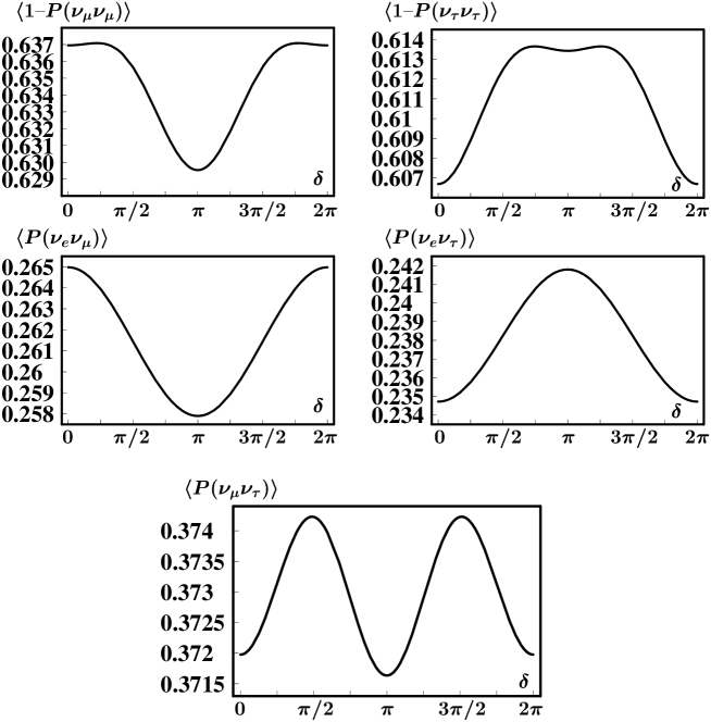
Figure 11: In this figure the dependences of the probabilities averaging over neutrino oscillations on the leptonic CP-phase are shown. These dependences are small and difference between maximal and minimal values of probabilities equals approximately $0.7\%$ in the $\nu_{\mu}\nu_{\mu}$ and $\nu_{\tau}\nu_{\tau}$ cases, $0.8\%$ in the $\nu_{e}\nu_{\mu}$ and $\nu_{e}\nu_{\tau}$ transitions and $0.03\%$ in the $\nu_{\mu}\nu_{\tau}$ transitions.

The second set of possible values for mixing angles taken from experimental data is:
example b)

$$\vartheta_{12}=(42.0\pm 2.0)^{\circ},\;\vartheta_{13}=(14.0\pm 1.0)^{\circ},\;\vartheta_{23}=(43.6\pm 0.5)^{\circ},$$ (179)

(this example is not in a good agreement with experimental data CHOOZ because, although it gives appropriate values for $\vartheta_{12}$ and $\vartheta_{23}$ (176), the value of $\vartheta_{13}$ is rather large here yap ).

In this case, i.e. at $\sin\vartheta_{13}=0.24$, coefficients $b_{ik},\,c_{ik}$ have larger values in comparison with the previous case. The values of these coefficients are of the order of several percent, in particular, $b_{e\mu}-b_{e\tau}\simeq 2b_{e\mu}\simeq 8.4\%$. So, we have in this case:

$$\left\{\begin{array}[]{l}A_{ee}=0.548;\\ A_{\mu\mu}=0.645,\;b_{\mu\mu}=0.019,\;c_{\mu\mu}=-0.044;\\ A_{\tau\tau}=0.627,\;b_{\tau\tau}=0.017,\;c_{\tau\tau}=-0.045;\\ A_{e\mu}=0.283,\;b_{e\mu}=0.041;\\ A_{e\tau}=0.265,\;b_{e\tau}=-0.043;\\ A_{\mu\tau}=0.348,\;b_{\mu\tau}=0.0077,\;c_{\mu\tau}=-0.0409.\end{array}\right.$$ (180)

Since $b_{e\mu}-b_{e\tau}\simeq 8.4\%$, the contribution of terms containing $\cos\delta_{l}$ to the ratio of probabilities $\langle P(\nu_{e}\nu_{\mu})\rangle$ and $\langle P(\nu_{e}\nu_{\tau})\rangle$ is of order of $8.4\%$. The results of corresponding measurements seem to be very interesting (see Fig.2).

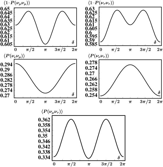
Figure 12: In this figure the dependences of the probabilities averaging over neutrino oscillations on the leptonic CP-phase are not so small as in the previous case (Fig.1.) because $\vartheta_{13}$ is not small and difference between maximal and minimal values of probabilities equals approximately $4\%$ in the $\nu_{\mu}\nu_{\mu}$ and $\nu_{\tau}\nu_{\tau}$ cases, $2.5\%$ in the $\nu_{e}\nu_{\mu}$ and $\nu_{e}\nu_{\tau}$ transitions and $2.8\%$ in the $\nu_{\mu}\nu_{\tau}$ transitions. Thus the role of $\vartheta_{13}$ in the manifestation of leptonic CP-phase in neutrino oscillations is very important.

30 The difference between the $\boldsymbol{\nu_{\alpha}\to\nu_{\beta}}$ transitions probability and the $\boldsymbol{\nu_{\beta}\to\nu_{\alpha}}$ transitions probability and leptonic CP-phase

Let us consider $\nu_{\alpha}\to\nu_{\beta}$ transitions in neutrino oscillations (denote them ”forward” transitions) and compare them with $\nu_{\beta}\to\nu_{\alpha}$ transitions (denote them ”backward” transitions). At $\delta_{l}\neq 0$ the probabilities of forward transitions differ from probabilities of backward transitions. Note right away that the probability of the forward transition coincides with the probability of the backward transition after averaging over all oscillations, while before averaging these probabilities are different provided CP-violating, i.e. at $\delta_{l}\neq 0$. And the difference between these probabilities is proportional to $\sin\delta_{l}$. These statements are direct consequences of general formulas for $P(\nu_{e}\nu_{\mu}),P(\nu_{e}\nu_{\tau})$ and $P(\nu_{\mu}\nu_{\tau})$ which given above. So, on obtaining probabilities of backward transitions by replacement $\delta_{l}\to-\delta_{l}$ we subtract probabilities of forward transitions from them. As a result we have:

$$\left\{\begin{array}[]{l}P(\nu_{\mu}\nu_{e})-P(\nu_{e}\nu_{\mu})=a_{0}(\sin\varphi_{21}+\sin\varphi_{32}-\sin\varphi_{31})\sin\delta_{l}\\ P(\nu_{\tau}\nu_{e})-P(\nu_{e}\nu_{\tau})=-a_{0}(\sin\varphi_{21}+\sin\varphi_{32}-\sin\varphi_{31})\sin\delta_{l}\\ P(\nu_{\tau}\nu_{\mu})-P(\nu_{\mu}\nu_{\tau})=a_{0}(\sin\varphi_{21}-2\sin\frac{\varphi_{21}}{2}\cos\frac{\displaystyle(\varphi_{31}+\varphi_{32})}{\displaystyle 2})\sin\delta_{l}\end{array}\right.$$ (181)

where $a_{0}=\frac{\displaystyle 1}{\displaystyle 2}c_{13}\sin 2\vartheta_{12}\sin 2\vartheta_{13}\sin 2\vartheta_{23}$. Here phases $\varphi_{21},\varphi_{32},\varphi_{31}$ depend on the time of neutrino flight in vacuum $t$ (see (171)) or, in other words, on distance (base-line) $L$ between points of neutrino birth and neutrino absorption and also on difference of squared masses $\Delta m_{ij}^{2}=m_{i}^{2}-m_{j}^{2}$. For the most possible values of neutrino masses and theirs average errors taken from experiment ispan ; camp :

$$m_{3}=(1/17\pm 1/50)eV,\;m_{2}=(1/175\pm 1/300)eV,\;m_{1}\ll m_{2}$$ (182)

We can see that the distance of the neutrino oscillations, i.e. the base-line for the experimental devices must not be less $10^{3}$m. The experimental definition of the CP-phase based on the correlation (181) would be the most natural, however now it is practically impossible because beams of different types (for example $\nu_{e}$ and $\nu_{\mu}$) of neutrino (that is, obtained in different reactions) but with the same energy are required for the experiment. This problem possibly will be solved in the future, but until now all experimental data were obtained only for beams of the neutrino with the continuous energy spectra. The cause of this problem consists, in particular, in very small cross-sections of neutrino interactions.

In current experiments we deal only with probabilities of transitions of neutrino with continuous energy spectra in the initial beam, i.e. with all phases (171) averaging over oscillations (174),(175) which also depend on the CP-violating phase $\delta_{l}$. The main idea of my talk consists in a suggestion to find the value of the CP-phase using data of experiments with large base-line and formulas (174),(175).

Note that coefficient $a_{0}$ defining the value of the effect of $t-$symmetry violating (181) is not too small in both $a)-$ and $b)-$cases:

$$a)\;a_{0}=0.07\qquad b)\;a_{0}=0.23$$

Moreover in b-case it is large. Therefore measurements of this effect are possible although they are difficult.

31 Conclusions.

So, the main results of our work are the following:

• The expressions for the probabilities of neutrino oscillations were obtained in the explicit form with regard for the leptonic CP-phase.

• The manifestation of the leptonic CP-phase in neutrino oscillations was investigated by the example of the probabilities averaging over oscillations. Using modern experimental data the model calculations and numerical estimates were done.

• The question of the $t-$symmetry violation for neutrino oscillation was analyzed. And there was established that the difference between the ”forward” probabilities and the ”backward” probabilities was proportional to sine of the leptonic CP-phase.

*Possibility of an Additional Source of Time Reversal Violation for Neutrinos R. ErdemE-mail:erdem@likya.iyte.edu.tr

32 Introduction

Topic of time reversal violation in neutrino processes (especially in oscillations) has gained much theoretical attention ref1 and there are proposals to study these effects experimentally ref2 . The main interest in these studies is to use T-violation as the measure of CP violation through fermion mixing matrices. In this study we show that the only source of time reversal violation in neutral fermion (hence in neutrino) processes is not the one which is related (through CPT theorem) to CP violation from complex phases in fermion mass matrices. There is an additional possible source of time reversal violation for neutral fermions arising from another kind of fermion mixing other than the Dirac and Majarona ones as we shall see below.

33 Four-component fermions and parity

Let us consider two 2-component fermions; $\chi_{1}$, $\chi_{2}$ which transform under the same representation of SL(2,C)

$$\chi_{1}\to e^{\frac{i}{2}\cdot(\mathchoice{\mbox{\boldmath$\displaystyle\theta$}}{\mbox{\boldmath$\textstyle\theta$}}{\mbox{\boldmath$\scriptstyle\theta$}}{\mbox{\boldmath$\scriptscriptstyle\theta$}}-i\mathchoice{\mbox{\boldmath$\displaystyle\nu$}}{\mbox{\boldmath$\textstyle\nu$}}{\mbox{\boldmath$\scriptstyle\nu$}}{\mbox{\boldmath$\scriptscriptstyle\nu$}})}\chi_{1},\qquad\chi_{2}\to e^{\frac{i}{2}\cdot(\mathchoice{\mbox{\boldmath$\displaystyle\theta$}}{\mbox{\boldmath$\textstyle\theta$}}{\mbox{\boldmath$\scriptstyle\theta$}}{\mbox{\boldmath$\scriptscriptstyle\theta$}}-i\mathchoice{\mbox{\boldmath$\displaystyle\nu$}}{\mbox{\boldmath$\textstyle\nu$}}{\mbox{\boldmath$\scriptstyle\nu$}}{\mbox{\boldmath$\scriptscriptstyle\nu$}})}\chi_{2}.$$ (183)

Assume that $\chi_{1}$, $\chi_{2}$ belong to different gauge groups or to different representations of the same gauge group. The simplest Lagrangian which can be constructed out of $\chi_{1}$, $\chi_{2}$ with related kinetic terms and quadratic interaction terms is

$${\cal L}=i\chi_{1}^{\dagger}\sigma_{\mu}D_{\mu}^{(1)}\chi_{1}+i\chi_{2}^{\dagger}\bar{\sigma}_{\mu}D_{\mu}^{(2)}\chi_{2}+m(\chi_{1}^{\dagger}i\sigma_{2}\chi_{2}^{*}+\chi_{2}^{\dagger}i\sigma_{2}\chi_{1}^{*})+h.c.$$ (184)

where h.c. stands for taking the complex conjugate of the terms preceeding it and $\sigma_{\mu}D_{\mu}=D_{0}\ \mathchoice{\mbox{\boldmath$\displaystyle\sigma$}}{\mbox{\boldmath$\textstyle\sigma$}}{\mbox{\boldmath$\scriptstyle\sigma$}}{\mbox{\boldmath$\scriptscriptstyle\sigma$}}\cdot\mathchoice{\mbox{\boldmath$\displaystyle D$}}{\mbox{\boldmath$\textstyle D$}}{\mbox{\boldmath$\scriptstyle D$}}{\mbox{\boldmath$\scriptscriptstyle D$}}$, $D_{\mu}^{(1)}=\partial_{\mu}+ig_{1}B_{\mu}^{(1)}$, $D_{\mu}^{(2)}=\partial_{\mu}+ig_{2}B_{\mu}^{(2)}$ with $B_{\mu}^{(1)}$, $B_{\mu}^{(2)}$ being the gauge fields coupling to $\chi_{1}$ and $\chi_{2}$, respectively. We assume an unbroken electromagnetic gauge group $U(1)_{em}$ . So $\chi_{1}$ , $\chi_{2}$ have opposite electric charges. Instead of identifying Eq.(184) as a Lagrangian of two (two-component) fermions interacting through a quadratic interaction term one may pass to a $4$-component formulation so that Eq.(184) becomes

$${\cal L}=i\bar{\psi}\not{D}^{(1)}P_{L}\psi+i\bar{\psi}\not{D}^{(2)}P_{R}\psi+m\bar{\psi}\psi+h.c.$$ (185)

Here

$$\psi=\begin{pmatrix}\chi_{1}\\ i\sigma_{2}\chi_{2}^{*}\end{pmatrix}=\begin{pmatrix}\chi_{L}\\ \chi_{R}\end{pmatrix},\quad\bar{\psi}=\psi^{\dagger}\gamma^{0},\quad P_{L}=\frac{1}{2}(1+\gamma_{5}),\quad P_{R}=\frac{1}{2}(1-\gamma_{5})$$ (186)

where in the chiral representation employed

$$\gamma_{5}=\begin{pmatrix}I&0\\ 0&-I\end{pmatrix}$$ (187)

The difference between Eq.(184) and Eq.(185) is that, in Eq.(185) there is a single $4$-component massive fermion while in Eq.(184) there are two interacting $2$-component massless fermions. So the $4$-component formulation simplifies the field theoretic calculations but the price to be paid is that the upper and lower two components transform under different gauge interactions. In fact this is one of the basic observations behind the parity violation in the standard model of electroweak interactions. Mathematically speaking the procedure given above where space reflection is associated with a $Z_{2}$ group corresponding to the exchange of the gauge group representations of left-handed and right-handed fermions is known as the method of group extensions ref3 . In particular here the procedure corresponds to the pullback of two $Z_{2}$ groups, one associated with space reflection and the other one associated with the exchange of the gauge group representations of the left-handed and right-handed fermions via the isomorphism relating the two $Z_{2}$ groups ref4 . In the next section we shall employ a similar procedure for time reversal.

A field theoretic formulation of these observations will make the picture clearer and more precise. First we take two $2$-component fermion fields, $\chi_{1}$ and $\chi_{2}$ (coupling through a quadratic interaction), with ref5

$$\chi_{1}=\int\frac{d^{3}p}{(2\pi)^{3/2}}\frac{1}{\sqrt{2E_{p}}}[u_{1}(\mathchoice{\mbox{\boldmath$\displaystyle p$}}{\mbox{\boldmath$\textstyle p$}}{\mbox{\boldmath$\scriptstyle p$}}{\mbox{\boldmath$\scriptscriptstyle p$}})b_{1}(\mathchoice{\mbox{\boldmath$\displaystyle p$}}{\mbox{\boldmath$\textstyle p$}}{\mbox{\boldmath$\scriptstyle p$}}{\mbox{\boldmath$\scriptscriptstyle p$}})e^{-ip\cdot x}+v_{1}(\mathchoice{\mbox{\boldmath$\displaystyle p$}}{\mbox{\boldmath$\textstyle p$}}{\mbox{\boldmath$\scriptstyle p$}}{\mbox{\boldmath$\scriptscriptstyle p$}})d_{1}^{\dagger}(\mathchoice{\mbox{\boldmath$\displaystyle p$}}{\mbox{\boldmath$\textstyle p$}}{\mbox{\boldmath$\scriptstyle p$}}{\mbox{\boldmath$\scriptscriptstyle p$}})e^{ip\cdot x}]$$

$$\chi_{2}=\int\frac{d^{3}p}{(2\pi)^{3/2}}\frac{1}{\sqrt{2E_{p}}}[u_{2}(\mathchoice{\mbox{\boldmath$\displaystyle p$}}{\mbox{\boldmath$\textstyle p$}}{\mbox{\boldmath$\scriptstyle p$}}{\mbox{\boldmath$\scriptscriptstyle p$}})b_{2}(\mathchoice{\mbox{\boldmath$\displaystyle p$}}{\mbox{\boldmath$\textstyle p$}}{\mbox{\boldmath$\scriptstyle p$}}{\mbox{\boldmath$\scriptscriptstyle p$}})e^{-ip\cdot x}+v_{2}(\mathchoice{\mbox{\boldmath$\displaystyle p$}}{\mbox{\boldmath$\textstyle p$}}{\mbox{\boldmath$\scriptstyle p$}}{\mbox{\boldmath$\scriptscriptstyle p$}})d_{2}^{\dagger}(\mathchoice{\mbox{\boldmath$\displaystyle p$}}{\mbox{\boldmath$\textstyle p$}}{\mbox{\boldmath$\scriptstyle p$}}{\mbox{\boldmath$\scriptscriptstyle p$}})e^{ip\cdot x}]$$ (188)

where $u_{1}$, $u_{2}$, $v_{1}$, $v_{2}$ are $2$-component spinors with $v_{1}\sim i\sigma_{2}u_{1}^{*}$, $v_{2}\sim i\sigma_{2}u_{2}^{*}$, $u_{2}\sim i\sigma_{2}u_{1}^{*}$, $v_{2}\sim i\sigma_{2}u_{2}^{*}$ and $b_{1}$, $b_{2}$, $d_{1}^{\dagger}$, $d_{2}^{\dagger}$ are the annihilation, creation operators for $\chi_{1}$ ,$\chi_{2}$ and $p\cdot x=E\cdot t-\mathchoice{\mbox{\boldmath$\displaystyle p$}}{\mbox{\boldmath$\textstyle p$}}{\mbox{\boldmath$\scriptstyle p$}}{\mbox{\boldmath$\scriptscriptstyle p$}}\cdot\mathchoice{\mbox{\boldmath$\displaystyle x$}}{\mbox{\boldmath$\textstyle x$}}{\mbox{\boldmath$\scriptstyle x$}}{\mbox{\boldmath$\scriptscriptstyle x$}}$. In the $4$-component formulation $\chi_{1}$ ,$\chi_{2}$ are replaced by a single $4$-component fermion with

$$\psi=\int\frac{d^{3}p}{(2\pi)^{3/2}}\frac{m}{\sqrt{E_{p}}}[u(\mathchoice{\mbox{\boldmath$\displaystyle p$}}{\mbox{\boldmath$\textstyle p$}}{\mbox{\boldmath$\scriptstyle p$}}{\mbox{\boldmath$\scriptscriptstyle p$}},\sigma)b(\mathchoice{\mbox{\boldmath$\displaystyle p$}}{\mbox{\boldmath$\textstyle p$}}{\mbox{\boldmath$\scriptstyle p$}}{\mbox{\boldmath$\scriptscriptstyle p$}},\sigma)e^{-ip\cdot x}+v(\mathchoice{\mbox{\boldmath$\displaystyle p$}}{\mbox{\boldmath$\textstyle p$}}{\mbox{\boldmath$\scriptstyle p$}}{\mbox{\boldmath$\scriptscriptstyle p$}},\sigma)d^{\dagger}(\mathchoice{\mbox{\boldmath$\displaystyle p$}}{\mbox{\boldmath$\textstyle p$}}{\mbox{\boldmath$\scriptstyle p$}}{\mbox{\boldmath$\scriptscriptstyle p$}},\sigma)e^{ip\cdot x}]$$ (189)

where $\sigma$ stands for either of helicity or spin. In the chiral basis ref5 ; ref6 ; ref7

$$u(\mathchoice{\mbox{\boldmath$\displaystyle p$}}{\mbox{\boldmath$\textstyle p$}}{\mbox{\boldmath$\scriptstyle p$}}{\mbox{\boldmath$\scriptscriptstyle p$}},1/2)=\begin{pmatrix}u_{1}\\ 0\end{pmatrix},\quad u(\mathchoice{\mbox{\boldmath$\displaystyle p$}}{\mbox{\boldmath$\textstyle p$}}{\mbox{\boldmath$\scriptstyle p$}}{\mbox{\boldmath$\scriptscriptstyle p$}},-1/2)=\begin{pmatrix}0\\ i\sigma_{2}v_{2}^{*}\end{pmatrix},$$

$$v(\mathchoice{\mbox{\boldmath$\displaystyle p$}}{\mbox{\boldmath$\textstyle p$}}{\mbox{\boldmath$\scriptstyle p$}}{\mbox{\boldmath$\scriptscriptstyle p$}},1/2)=\begin{pmatrix}v_{1}\\ 0\end{pmatrix},\quad v(\mathchoice{\mbox{\boldmath$\displaystyle p$}}{\mbox{\boldmath$\textstyle p$}}{\mbox{\boldmath$\scriptstyle p$}}{\mbox{\boldmath$\scriptscriptstyle p$}},-1/2)=\begin{pmatrix}0\\ i\sigma_{2}u_{2}^{*}\end{pmatrix}$$ (190)

$$b(\mathchoice{\mbox{\boldmath$\displaystyle p$}}{\mbox{\boldmath$\textstyle p$}}{\mbox{\boldmath$\scriptstyle p$}}{\mbox{\boldmath$\scriptscriptstyle p$}},1/2)=b_{1}(\mathchoice{\mbox{\boldmath$\displaystyle p$}}{\mbox{\boldmath$\textstyle p$}}{\mbox{\boldmath$\scriptstyle p$}}{\mbox{\boldmath$\scriptscriptstyle p$}}),\quad b(\mathchoice{\mbox{\boldmath$\displaystyle p$}}{\mbox{\boldmath$\textstyle p$}}{\mbox{\boldmath$\scriptstyle p$}}{\mbox{\boldmath$\scriptscriptstyle p$}},-1/2)=d_{2}(\mathchoice{\mbox{\boldmath$\displaystyle p$}}{\mbox{\boldmath$\textstyle p$}}{\mbox{\boldmath$\scriptstyle p$}}{\mbox{\boldmath$\scriptscriptstyle p$}}),$$

$$d(\mathchoice{\mbox{\boldmath$\displaystyle p$}}{\mbox{\boldmath$\textstyle p$}}{\mbox{\boldmath$\scriptstyle p$}}{\mbox{\boldmath$\scriptscriptstyle p$}},1/2)=d_{1}(\mathchoice{\mbox{\boldmath$\displaystyle p$}}{\mbox{\boldmath$\textstyle p$}}{\mbox{\boldmath$\scriptstyle p$}}{\mbox{\boldmath$\scriptscriptstyle p$}}),\quad d(\mathchoice{\mbox{\boldmath$\displaystyle p$}}{\mbox{\boldmath$\textstyle p$}}{\mbox{\boldmath$\scriptstyle p$}}{\mbox{\boldmath$\scriptscriptstyle p$}},-1/2)=b_{2}(\mathchoice{\mbox{\boldmath$\displaystyle p$}}{\mbox{\boldmath$\textstyle p$}}{\mbox{\boldmath$\scriptstyle p$}}{\mbox{\boldmath$\scriptscriptstyle p$}})$$

where $\pm 1/2$ stands for different helicity states. In the mass basis (which is the solution basis for the Dirac equation) ref8 one may write

$$[u(\mathchoice{\mbox{\boldmath$\displaystyle p$}}{\mbox{\boldmath$\textstyle p$}}{\mbox{\boldmath$\scriptstyle p$}}{\mbox{\boldmath$\scriptscriptstyle p$}},\sigma)b(\mathchoice{\mbox{\boldmath$\displaystyle p$}}{\mbox{\boldmath$\textstyle p$}}{\mbox{\boldmath$\scriptstyle p$}}{\mbox{\boldmath$\scriptscriptstyle p$}},\sigma)e^{-ip\cdot x}+v(\mathchoice{\mbox{\boldmath$\displaystyle p$}}{\mbox{\boldmath$\textstyle p$}}{\mbox{\boldmath$\scriptstyle p$}}{\mbox{\boldmath$\scriptscriptstyle p$}},\sigma)d^{\dagger}(\mathchoice{\mbox{\boldmath$\displaystyle p$}}{\mbox{\boldmath$\textstyle p$}}{\mbox{\boldmath$\scriptstyle p$}}{\mbox{\boldmath$\scriptscriptstyle p$}},\sigma)e^{ip\cdot x}]$$

$$=\begin{pmatrix}(u_{1}+i\sigma_{2}u_{1}^{*})b_{1}+(v_{2}+i\sigma_{2}v_{2}^{*})d_{2}\\ (i\sigma_{2}v_{2}^{*}-v_{2})d_{2}+(i\sigma_{2}u_{1}^{*}-u_{1})b_{1}\end{pmatrix}e^{-ip\cdot x}$$ (191)

$$+\begin{pmatrix}(-v_{1}+i\sigma_{2}v_{1})d_{1}^{\dagger}+(u_{2}-i\sigma_{2}u_{2}^{*})b_{2}^{\dagger}\\ (u_{2}+i\sigma_{2}u_{2}^{*})b_{2}^{\dagger}+(v_{1}+i\sigma_{2}v_{1}^{*})d_{1}^{\dagger}\end{pmatrix}e^{ip\cdot x}$$

which is a sum of two independent spin states.

The lower and upper two components of $\psi$ in the chiral representation, $\chi_{L}$ and $\chi_{R}$ are related by space reflection and interchange of $\chi_{L}$ and $\chi_{R}$ amounts to a space reflection operation plus interchange of the gauge group representations of $\chi_{L}$ and $\chi_{R}$ ref9 . This is the case because in the $4$-component formulation $\chi_{L}$ and $\chi_{R}$ form a single system $\psi$ so their interchanges are mutually related to each other. In the next section we shall investigate such a possibility for time reversal. We shall couple two $4$-component fermions (with different gauge group representations) through a quadratic coupling where each $4$-component fermion in the coupling can be redefined so that each is the time reversal of the other. Then the result is a single system i.e. an $8$-component fermion consisting of the original $4$-component fermions. In this way time reversal is associated with the interchange of the gauge group representations of the original two $4$-component fermions. This, in turn, enables one to break the time reversal invariance in a way other than the complex phases in the fermion mixing matrices.

34 $8$-component fermions and time reversal

In the previous section we have seen that one can interprete a quadratic interaction term between two $2$-component massless fermions as a fermion mass term by passing to $4$-component fermion formulation. In this section we raise the question if one can find a Lorentz invariant quadratic term, other than the mass term for $4$-component fermions, between two $4$-component fermions, which can be interpreted as a mass term for $8$-component fermions. We shall see that this possible provided the fermion is neutral and massless ( or almost massless) and the upper and lower two components of these $8$-component fermions are related by time reversal. This observation opens up the possibility of an additional source of time reversal violation for neutral fermions in a way similar to the case of parity for $4$-component formulation.

We consider two $4$-component fermions given by

$$\psi_{1} = \sum_{\sigma}\int\frac{d^{3}p}{(2\pi)^{3/2}}\frac{1}{\sqrt{2E_{p}}}[u_{1}(\mathchoice{\mbox{\boldmath$\displaystyle p$}}{\mbox{\boldmath$\textstyle p$}}{\mbox{\boldmath$\scriptstyle p$}}{\mbox{\boldmath$\scriptscriptstyle p$}})b_{1}(\mathchoice{\mbox{\boldmath$\displaystyle p$}}{\mbox{\boldmath$\textstyle p$}}{\mbox{\boldmath$\scriptstyle p$}}{\mbox{\boldmath$\scriptscriptstyle p$}})e^{-ip\cdot x}+v_{1}(\mathchoice{\mbox{\boldmath$\displaystyle p$}}{\mbox{\boldmath$\textstyle p$}}{\mbox{\boldmath$\scriptstyle p$}}{\mbox{\boldmath$\scriptscriptstyle p$}})d_{1}^{\dagger}(\mathchoice{\mbox{\boldmath$\displaystyle p$}}{\mbox{\boldmath$\textstyle p$}}{\mbox{\boldmath$\scriptstyle p$}}{\mbox{\boldmath$\scriptscriptstyle p$}})e^{ip\cdot x}]$$

$$\psi_{2} = \sum_{\sigma}\int\frac{d^{3}p}{(2\pi)^{3/2}}\frac{1}{\sqrt{2E_{p}}}[u_{2}(\mathchoice{\mbox{\boldmath$\displaystyle p$}}{\mbox{\boldmath$\textstyle p$}}{\mbox{\boldmath$\scriptstyle p$}}{\mbox{\boldmath$\scriptscriptstyle p$}})b_{2}(\mathchoice{\mbox{\boldmath$\displaystyle p$}}{\mbox{\boldmath$\textstyle p$}}{\mbox{\boldmath$\scriptstyle p$}}{\mbox{\boldmath$\scriptscriptstyle p$}})e^{-ip\cdot x}+v_{2}(\mathchoice{\mbox{\boldmath$\displaystyle p$}}{\mbox{\boldmath$\textstyle p$}}{\mbox{\boldmath$\scriptstyle p$}}{\mbox{\boldmath$\scriptscriptstyle p$}})d_{2}^{\dagger}(\mathchoice{\mbox{\boldmath$\displaystyle p$}}{\mbox{\boldmath$\textstyle p$}}{\mbox{\boldmath$\scriptstyle p$}}{\mbox{\boldmath$\scriptscriptstyle p$}})e^{ip\cdot x}]$$ (192)

$u_{1}$, $u_{2}$, $v_{1}$, $v_{2}$ are, this time, $4$-component spinors with the spinor parts of $\psi_{1}$, $\psi_{2}$ being each others time reversals i.e.

$$u_{2}(\mathchoice{\mbox{\boldmath$\displaystyle p$}}{\mbox{\boldmath$\textstyle p$}}{\mbox{\boldmath$\scriptstyle p$}}{\mbox{\boldmath$\scriptscriptstyle p$}},\sigma)\sim i\gamma^{1}\gamma^{3}u_{1}^{*}(\mathchoice{\mbox{\boldmath$\displaystyle p$}}{\mbox{\boldmath$\textstyle p$}}{\mbox{\boldmath$\scriptstyle p$}}{\mbox{\boldmath$\scriptscriptstyle p$}},\sigma),\quad v_{2}(\mathchoice{\mbox{\boldmath$\displaystyle p$}}{\mbox{\boldmath$\textstyle p$}}{\mbox{\boldmath$\scriptstyle p$}}{\mbox{\boldmath$\scriptscriptstyle p$}},\sigma)\sim i\gamma^{1}\gamma^{3}v_{1}^{*}(\mathchoice{\mbox{\boldmath$\displaystyle p$}}{\mbox{\boldmath$\textstyle p$}}{\mbox{\boldmath$\scriptstyle p$}}{\mbox{\boldmath$\scriptscriptstyle p$}},\sigma)$$ (193)

The only possible Lorentz invariant quadratic interaction term between $\psi_{1}$ and $\psi_{2}$ is ref10

$$M(\psi_{1}^{\dagger}\psi_{2}+\psi_{2}^{\dagger}\psi_{1})$$ (194)

The simplest possible Lagrangian reads

$${\cal L}=i\bar{\psi}_{1}\not{D}^{(1)}\psi_{1}-i\bar{\psi}_{2}\gamma^{0}\psi_{2}+m\bar{\psi}_{1}\bar{\psi}_{1}+m\bar{\psi}_{2}\bar{\psi}_{2}+M(\psi_{1}^{\dagger}\psi_{2}+\psi_{2}^{\dagger}\psi_{1})+h.c.$$ (195)

where $\not{D}^{(1)}=\gamma^{\mu}(\partial_{\mu}-ig_{1}B_{\mu}^{(1)})$, $\not{D}^{(2)}=\gamma^{\mu}(\partial_{\mu}-ig_{2}B_{\mu}^{(2)})$. We take both $\psi_{1}$ and $\psi_{2}$ be massless (for example through a chiral symmetry). Then (195) can be put into a simple $8$-component form

$${\cal L}=i\bar{\Psi}\not{\cal D}^{(1)}P_{U}\Psi+i\bar{\Psi}\not{\cal D}^{(2)}P_{D}\Psi+M\bar{\Psi}\Psi+h.c.$$ (196)

where

$${\cal D}=\begin{pmatrix}0&-\not{D}\gamma^{0}\\ \gamma^{0}\not{D}&0\end{pmatrix},\quad P_{U}=\begin{pmatrix}I_{4}&0\\ 0&0\end{pmatrix},\quad P_{D}=\begin{pmatrix}0&0\\ 0&I_{4}\end{pmatrix},$$

$$\Psi=\begin{pmatrix}\psi_{1}\\ \psi_{2}\end{pmatrix},\qquad\bar{\Psi}=\Psi^{\dagger}\tilde{\Gamma},\qquad\tilde{\Gamma}=\begin{pmatrix}0&I_{4}\\ i_{4}&0\end{pmatrix}$$ (197)

So $\Psi$ acts as a single fermion whose upper and lower $4$-components couple to different gauge groups, and the spinor parts of the lower and the upper components are related by time reversal. Because the spinor parts of $\psi_{1}$ , $\psi_{2}$ are related by time reversal $\psi_{2}$ has the same electric charge as $\psi_{1}$ . However because time reversal is violated (for example through weak interactions) there will be an effective charge asymmetry induced between $\chi_{1}$ and $\chi_{2}$ which forbids $\psi_{1}^{\dagger}\psi_{2}$ type of terms. This requires that $\Psi$ should be a neutral particle in order to allow $\psi_{1}^{\dagger}\psi_{2}$ type of terms (provided the electric charge is a conserved quantity). In summary the Lagrangian (196) is applicable only for neutral particles and in that case there is an additional source of time reversal violation other than the one due to the complex phases in the fermion mixing matrix. If one assigns one of the $\psi_{1}$, $\psi_{2}$ to the singlet and the other to a nontrivial representation of the gauge group then the time reversal becomes maximal in the same way as in the standard model of electroweak interactions. The propagator of $\Psi$ corresponding to Eq. (196) is

$$\frac{i}{\Gamma^{\mu}p_{\mu}-M}\qquad\mbox{where}\qquad\Gamma^{\mu}=\begin{pmatrix}0&-\gamma^{\mu}\gamma^{0}\\ \gamma^{0}\gamma^{\mu}&0\end{pmatrix}$$ (198)

If we take $m_{1}=m_{2}=m\simeq 0$ then the mass terms of $\psi_{1}$, $\psi_{2}$ behave as quadratic interaction terms which modify the propagator self energy contribution which changes $MI_{8}$ to $MI_{8}+\gamma^{0}m\tilde{\Gamma}$ where $I_{8}$ stands for $8\times 8$ unit matrix. In this case $\Psi$ can be still considered as a single fermionic system with some perturbative self interaction term.

The parity and time reversal operators in this case can be infered more easily by considering the Dirac and the Dirac-like equations corresponding to the Lagrangians (185) and (196)

$$i\not{D}^{(1)}P_{L}\psi+mP_{R}\psi=0,\qquad i\not{D}^{(2)}P_{R}\psi+mP_{L}\psi=0$$ (199)

$$i\not{D}^{(1)}P_{U}\psi+MP_{D}\psi=0,\qquad i\not{D}^{(2)}P_{D}\psi+MP_{U}\psi=0$$ (200)

One can determine the parity and time reversal operators by letting $\mathchoice{\mbox{\boldmath$\displaystyle x$}}{\mbox{\boldmath$\textstyle x$}}{\mbox{\boldmath$\scriptstyle x$}}{\mbox{\boldmath$\scriptscriptstyle x$}}\to-\mathchoice{\mbox{\boldmath$\displaystyle x$}}{\mbox{\boldmath$\textstyle x$}}{\mbox{\boldmath$\scriptstyle x$}}{\mbox{\boldmath$\scriptscriptstyle x$}}$ and $t\to-t$, respectively, in the equations given above. One notices that there are more than one operator acting on the fields corresponding to each of these transformations. For example, for parity one may take either of

$$\begin{pmatrix}\gamma^{0}&0\\ 0&\gamma^{0}\end{pmatrix},\qquad\Gamma^{0}=\begin{pmatrix}0&-I\\ I&0\end{pmatrix}$$ (201)

for time reversal either of

$$\begin{pmatrix}i\gamma^{1}\gamma^{3}\;K&0\\ 0&i\gamma^{1}\gamma^{3}\;K\end{pmatrix},\qquad\tilde{\Gamma}=\begin{pmatrix}0&I\\ I&0\end{pmatrix}$$ (202)

where $K$ stands for complex conjugation of c-numbers on its right hand side. Here the first operators in (201) and (202) correspond to the direct extension of the usual parity and time reversal operators for the $8$-component case. One notices that the second time reversal operator in (202) is unitary. At first sight this seems to contradict with the Wigner’s requirement that time reversal is a symmetry of the physical systems so it should be anti-unitary ref11 . However Wigner’s argument assumes that the time reversal of an operator corresponding to a physical observable $Q$ at time $t$, $Q(t)=exp(iHt)Qexp(-iHt)$ is given by $exp(-iHt)Qexp(iHt)$. In other words he implicitly assumes that the Hamiltonian $H$ is invariant under time reversal. Because the additional time reversal operator in (202) only applies to neutrinos (whose time reversal properties are not well known) and it does not leave the Hamiltonian invariant in general (its violation may be even maximal) so the Wigner’s argument does not apply to the present case.

While both operators in (201) or (202) correspond to the same space-time reflection the physical operations to perform these transformations are different. In other words the experiments designed to study parity or time reversal in a physical process are different in each case. The parity transformation corresponding to the first operator in (201) is accomplished by interchange of the left-handed and right-handed components of the $4$-component fermions. Because this interchange is associated with space reflection and each of left-handed and right-handed components are associated with opposite helicities one can check parity invariance under this operation by checking the space reflection in a given fermionic process. However the second operation in (201) does not correspond to a simple exchange of the left-handed and right-handed components so it corresponds to preparing a different experiment where the state vectors for the fermions are transformed accordingly. In other words it is not possible to test the invariance of parity due to the second transformation in (201) by checking space reflection invariance in the same fermionic process, i.e. in this case one should first study the original process and then the process corresponding to the parity transformed one. A similar argument is true for the time reversal operators in Eq.(202). The first (the one which corresponds to the usual time reversal) corresponds to preparing a different process which corresponds to the time reversed of the original process while the test of time reversal for the second operator can be achieved, in principle, in the same process by comparing the intensity of the events in the direction forward in time and the events in the direction backward in time. While this is not applicable in practice one may test the time reversal in the same process in this case in indirect ways. The spinor part of $\Psi$, $U$ can be written in the following way

$$U=\begin{pmatrix}U_{1}\\ U_{2}\end{pmatrix},\qquad U_{1}=\begin{pmatrix}u_{1}^{(1)}\\ u_{2}^{(1)}\end{pmatrix},\qquad U_{2}=\begin{pmatrix}u_{1}^{(2)}\\ u_{2}^{(2)}\end{pmatrix},$$ (203)

In the chiral basis the components of $U$ may be related as ref9 ; ref12

$$u_{1}^{(1)}=\frac{1}{m}(p_{0}+\mathchoice{\mbox{\boldmath$\displaystyle\sigma$}}{\mbox{\boldmath$\textstyle\sigma$}}{\mbox{\boldmath$\scriptstyle\sigma$}}{\mbox{\boldmath$\scriptscriptstyle\sigma$}}\cdot\mathchoice{\mbox{\boldmath$\displaystyle p$}}{\mbox{\boldmath$\textstyle p$}}{\mbox{\boldmath$\scriptstyle p$}}{\mbox{\boldmath$\scriptscriptstyle p$}})u_{2}^{(1)},\qquad u_{1}^{(2)}=\frac{1}{m}(p_{0}-\mathchoice{\mbox{\boldmath$\displaystyle\sigma$}}{\mbox{\boldmath$\textstyle\sigma$}}{\mbox{\boldmath$\scriptstyle\sigma$}}{\mbox{\boldmath$\scriptscriptstyle\sigma$}}\cdot\mathchoice{\mbox{\boldmath$\displaystyle p$}}{\mbox{\boldmath$\textstyle p$}}{\mbox{\boldmath$\scriptstyle p$}}{\mbox{\boldmath$\scriptscriptstyle p$}})u_{2}^{(2)}$$

$$u_{1}^{(1)}=\frac{1}{m}(-p_{0}+\mathchoice{\mbox{\boldmath$\displaystyle\sigma$}}{\mbox{\boldmath$\textstyle\sigma$}}{\mbox{\boldmath$\scriptstyle\sigma$}}{\mbox{\boldmath$\scriptscriptstyle\sigma$}}\cdot\mathchoice{\mbox{\boldmath$\displaystyle p$}}{\mbox{\boldmath$\textstyle p$}}{\mbox{\boldmath$\scriptstyle p$}}{\mbox{\boldmath$\scriptscriptstyle p$}})u_{1}^{(2)},\qquad u_{2}^{(1)}=\frac{1}{m}(-p_{0}-\mathchoice{\mbox{\boldmath$\displaystyle\sigma$}}{\mbox{\boldmath$\textstyle\sigma$}}{\mbox{\boldmath$\scriptstyle\sigma$}}{\mbox{\boldmath$\scriptscriptstyle\sigma$}}\cdot\mathchoice{\mbox{\boldmath$\displaystyle p$}}{\mbox{\boldmath$\textstyle p$}}{\mbox{\boldmath$\scriptstyle p$}}{\mbox{\boldmath$\scriptscriptstyle p$}})u_{2}^{(2)}$$ (204)

We notice that both $\psi_{1}$ and $\psi_{2}$ have exactly the same helicities. So if two kinds of neutrinos are produced which have the same helicities and which do not interact with one another through gauge interactions (due to Lorentz invariance) one may suspect if these additional neutrinos are $\psi_{2}$’s (provided $\psi_{1}$’s are identified by the usual neutrinos). If the interaction of $\Psi$’s is time reversal invariant under electroweak interactions then the presence of additional neutrinos (i.e. $\psi_{2}$’s) are seen as an extra factor of $2$ in the production cross sections of neutrinos when compared with their interaction with $Z$ bosons. If there is a time reversal violation then this may either be due to the usual source of time reversal violation arising from complex phase(s) in fermion mixing matrices or it may be due to non-invariance under the interchanges of $\psi_{1}$ and $\psi_{2}$. Seeking for any asymmetry between the gauge interactions of $\psi_{1}$’s and $\psi_{2}$’s in the same process amounts to seeking a time reversal violation due to the second operator in Eq(202). However it may not be easy to disentagle these two types of time reversal violation.

35 Conclusion

We have seen that as in the case of parity one may extend time reversal operator by a $Z_{2}$ group associated with the interchange of the gauge group representations of two coupled fermions whose spinor parts are time reversals of each other. In this way one gets the possibility of an additional source of time reversal violation for neutral fermions (e.g for neutrinos). This time reversal violation is similiar to the parity violation and it may be even maximal as in the case of parity. If this additional time reversal has a comparable magnitude as the usual time reversal violation resulting from complex phase(s) in fermion mass matrices then the mixing phase can not be direcly derived from the magnitude of time reversal violation and vica versa. The presence of the extra time reversal violation can be infered by comparing the magnitudes of the time reversal and the usual CP violation in a neutrino process (for example in neutrino oscillations) in future experiments.

*Quark-Lepton Masses and the Neutrino Puzzle in the AGUT Model C.D. Froggatt

36 Introduction

I reviewed the general problem of the quark-lepton mass spectrum at the first Bled workshop on “What comes beyond the Standard Model” bled1 . So, in this talk, I will mainly concentrate on two topics: the Lightest Flavour Mass Generation model and the Neutrino Mass and Mixing problem in the Anti-Grand Unification Theory (AGUT).

37 Lightest Flavour Mass Generation Model

A commonly accepted framework for discussing the flavour problem is based on the picture that, in the absence of flavour mixing, only the particles belonging to the third generation $t$, $b$ and $\tau$ have non-zero masses. All other masses and the mixing angles then appear as a result of the tree-level mixings of families, related to some underlying family symmetry breaking. Recently, a new mechanism of flavour mixing, which we call Lightest Family Mass Generation (LFMG), was proposed lfm . According to LFMG the whole of flavour mixing for quarks is basically determined by the mechanism responsible for generating the physical masses of the up and down quarks, $m_{u}$ and $m_{d}$ respectively. So, in the chiral symmetry limit, when $m_{u}$ and $m_{d}$ vanish, all the quark mixing angles vanish. Therefore, the masses (more precisely any of the diagonal elements of the quark and charged lepton mass matrices) of the second and third families are practically the same in the gauge (unrotated) and physical bases. The proposed flavour mixing mechanism, driven solely by the generation of the lightest family mass, could actually be realized in two generic ways.

The first basic alternative (I) is when the lightest family mass ($m_{u}$ or $m_{d}$) appears as a result of the complex flavour mixing of all three families. It “runs along the main diagonal” of the corresponding $3\times 3$ mass matrix $M$, from the basic dominant element $M_{33}$ to the element $M_{22}$ (via a rotation in the 2-3 sub-block of $M$) and then to the primordially texture zero element $M_{11}$ (via a rotation in the 1-2 sub-block). The direct flavour mixing of the first and third quark and lepton families is supposed to be absent or negligibly small in $M$.

The second alternative (II), on the contrary, presupposes direct flavour mixing of just the first and third families. There is no involvement of the second family in the mixing. In this case, the lightest mass appears in the primordially texture zero $M_{11}$ element “walking round the corner” (via a rotation in the 1-3 sub-block of the mass matrix $M$). Certainly, this second version of the LFMG mechanism cannot be used for both the up and the down quark families simultaneously, since mixing with the second family members is a basic part of the CKM quark mixing phenomenology (Cabibbo mixing, non-zero $V_{cb}$ element, CP violation). However, the alternative II could work for the up quark family provided that the down quarks follow the alternative I.

Here we will just consider the latter scenario.

37.1 Quark Sector

We propose that the mass matrix for the down quarks ($D$ = $d$, $s$, $b$) is Hermitian with three texture zeros of the following alternative I form:

$$M_{D}=\begin{pmatrix}0&a_{D}&0\\ a_{D}^{\ast}&A_{D}&b_{D}\\ 0&b_{D}^{\ast}&B_{D}\end{pmatrix}$$ (205)

It is, of course, necessary to assume some hierarchy between the elements, which we take to be: $B_{D}\gg A_{D}\sim\left|b_{D}\right|\gg\left|a_{D}\right|$. The zero in the $\left(M_{D}\right)_{11}$ element corresponds to the commonly accepted conjecture that the lightest family masses appear as a direct result of flavour mixings. The zero in $\left(M_{D}\right)_{13}$ means that only minimal “nearest neighbour” interactions occur, giving a tridiagonal matrix structure.

Now our main hypothesis, that the second and third family diagonal mass matrix elements are practically the same in the gauge and physical quark-lepton bases, means that :

$$B_{D}=m_{b}+\delta_{D}\qquad A_{D}=m_{s}+\delta_{D}^{\prime}$$ (206)

The components $\delta_{D}$ and $\delta_{D}^{\prime}$ are supposed to be much less than the masses of the particles in the next lightest family, meaning:

$$|\delta_{D}|\ll m_{s}\qquad|\delta_{D}^{\prime}|\ll m_{d}$$ (207)

Since the trace and determinant of the Hermitian matrix $M_{D}$ gives the sum and product of its eigenvalues, it follows that

$$\delta_{D}\simeq-m_{d}$$ (208)

while $\delta_{D}^{\prime}$ is vanishingly small and can be neglected in further considerations.

It may easily be shown that our hypothesis and related equations (206 - 208) are entirely equivalent to the condition that the diagonal elements ($A_{D}$, $B_{D}$) of $M_{D}$ are proportional to the modulus square of the off-diagonal elements ($a_{D}$, $b_{D}$):

$$\frac{A_{D}}{B_{D}}=\left|\frac{a_{D}}{b_{D}}\right|^{2}$$ (209)

Using the conservation of the trace, determinant and sum of principal minors of the Hermitian matrices $M_{D}$ under unitary transformations, we are led to a complete determination of the moduli of all their elements, which can be expressed to high accuracy as follows:

$$\left|M_{D}\right|=\begin{pmatrix}0&\sqrt{m_{d}m_{s}}&0\\ \sqrt{m_{d}m_{s}}&m_{s}&\sqrt{m_{d}m_{b}}\\ 0&\sqrt{m_{d}m_{b}}&m_{b}-m_{d}\end{pmatrix}$$ (210)

Now the Hermitian mass matrix for the up quarks is taken to be of the following alternative II form:

$$M_{U}=\begin{pmatrix}0&0&c_{U}\\ 0&A_{U}&0\\ c_{U}^{\ast}&0&B_{U}\end{pmatrix}$$ (211)

The moduli of all the elements of $M_{U}$ can also be readily determined in terms of the physical masses as follows:

$$\left|M_{U}\right|=\begin{pmatrix}0&0&\sqrt{m_{u}m_{t}}\\ 0&m_{c}&0\\ \sqrt{m_{u}m_{t}}&0&m_{t}-m_{u}\end{pmatrix}$$ (212)

The CKM quark mixing matrix elements can now be readily calculated by diagonalising the mass matrices $M_{D}$ and $M_{U}$. They are given by the following simple and compact formulae in terms of quark mass ratios:

$$\left|V_{us}\right|=\sqrt{\frac{m_{d}}{m_{s}}}=0.222\pm 0.004\qquad\left|V_{us}\right|_{exp}=0.221\pm 0.003$$ (213)

$$\left|V_{cb}\right|=\sqrt{\frac{m_{d}}{m_{b}}}=0.038\pm 0.004\qquad\left|V_{cb}\right|_{exp}=0.039\pm 0.003$$ (214)

$$\left|V_{ub}\right|=\sqrt{\frac{m_{u}}{m_{t}}}=0.0036\pm 0.0006\qquad\left|V_{ub}\right|_{exp}=0.0036\pm 0.0006$$ (215)

As can be seen, they are in impressive agreement with the experimental values.

37.2 Lepton Sector

The MNS lepton mixing matrix is defined analogously to the CKM quark mixing matrix:

$$U=U_{\nu}U{{}_{E}}^{\dagger}$$ (216)

Here $U_{E}$ and $U_{\nu}$ are the unitary matrices which diagonalise the charged lepton mass matrix $M_{E}$ and the effective neutrino mass matrix $M_{\nu}$ respectively. Assuming the charged lepton masses follow alternative I, like the down quarks, the LFMG model predicts the charged lepton mixing angles in the matrix $U_{E}$ to be:

$$\sin\theta_{e\mu}=\sqrt{\frac{m_{e}}{m_{\mu}}}\qquad\sin\theta_{\mu\tau}=\sqrt{\frac{m_{e}}{m_{\tau}}}\qquad\sin\theta_{e\tau}\simeq 0$$ (217)

These small charged lepton mixing angles will not markedly effect atmospheric neutrino oscillations, which appear to require maximal mixing $\sin^{2}2\theta_{atm}\simeq 1$. Similarly, in the case of the large mixing angle (LMA) MSW solution of the solar neutrino problem, they are essentially negligible. It follows then that the large neutrino mixings should mainly come from the $U_{\nu}$ matrix associated with the neutrino mass matrix.

According to the “see-saw” mechanism, the effective mass-matrix $M_{\nu}$ for physical neutrinos has the form

$$M_{\nu}=-M_{N}^{T}M_{NN}^{-1}M_{N}$$ (218)

where $M_{N}$ is their Dirac mass matrix, while $M_{NN}$ is the Majorana mass matrix of their right-handed components. Matsuda et al refs have extended the alternative I LFMG texture to the Dirac $M_{N}$ and Majorana $M_{NN}$ matrices.

The eigenvalues of the neutrino Dirac mass matrix $M_{N}$ are taken to have a hierarchy similar to that for the charged leptons (and down quarks)

$$M_{N3}:M_{N2}:M_{N1}\simeq 1:y^{2}:y^{4},\quad y\approx 0.1$$ (219)

and the eigenvalues of the Majorana mass matrix $M_{NN}$ are taken to have a stronger hierarchy

$$M_{NN3}:M_{NN2}:M_{NN1}\simeq 1:y^{4}:y^{6}$$ (220)

One then readily determines the general LFMG matrices $M_{N}$ and $M_{NN}$ to be of the type

$$M_{N}\simeq M_{N3}\left(\begin{array}[]{lll}0&\alpha y^{3}&0\\ \alpha y^{3}&y^{2}&\alpha y^{2}\\ 0&\alpha y^{2}&1\end{array}\right)$$ (221)

and

$$M_{NN}\simeq M_{NN3}\left(\begin{array}[]{lll}0&\beta y^{5}&0\\ \beta y^{5}&y^{4}&\beta y^{3}\\ 0&\beta y^{3}&1\end{array}\right).$$ (222)

We further take an extra condition of the type

$$\left|\Delta-1\right|\leq y^{2}\qquad(\Delta\equiv\alpha,\beta)$$ (223)

for both the order-one parameters $\alpha$ and $\beta$ contained in the matrices $M_{N}$ and $M_{NN}$, according to which they are supposed to be equal to unity with a few percent accuracy. Substitution in the seesaw formula (218) generates an effective physical neutrino mass matrix $M_{\nu}$ of the form:

$$M_{\nu}\simeq-\frac{M_{N3}^{2}}{M_{NN3}}\left(\begin{array}[]{lll}0&y&0\\ y&1+(y-y^{2})^{2}&1-(y-y^{2})\\ 0&1-(y-y^{2})&1\end{array}\right)$$ (224)

The physical neutrino masses are then given by:

$$m_{\nu 1} \simeq (\frac{1}{2}-\frac{\sqrt{3}}{2})\frac{M_{N3}^{2}}{M_{NN3}}\cdot y,$$

$$m_{\nu 2} \simeq (\frac{1}{2}+\frac{\sqrt{3}}{2})\frac{M_{N3}^{2}}{M_{NN3}}\cdot y,\quad m_{\nu 3}\simeq(2-y)\frac{M_{N3}^{2}}{M_{NN3}}$$ (225)

The predicted values of the neutrino oscillation parameters are:

$$\sin^{2}2\theta_{atm}\simeq 1,\quad\sin^{2}2\theta_{sun}\simeq\frac{2}{3},\quad U_{e3}\simeq\frac{1}{2\sqrt{2}}y,\quad\frac{\Delta m_{sun}^{2}}{\Delta m_{atm}^{2}}\simeq\frac{\sqrt{3}}{4}y^{2}$$ (226)

in agreement with atmospheric and LMA-MSW solar neutrino oscillation data.

The proportionality condition (209), which leads to the LFMG texture, is not so easy to generate from an underlying symmetry beyond the Standard Model. However Jon Chkareuli, Holger Nielsen and myself have recently shown SU3 that it is possible to give a natural realisation of the LFMG texture in a local chiral $SU(3)$ family symmetry model.

38 Fermion Masses in the AGUT Model

The AGUT model is based on a non-simple extension of the Standard Model (SM) with three copies of the SM gauge group—one for each family—and, in the absence of right-handed neutrinos, one extra abelian factor: $G=SMG^{3}\times U(1)_{f}$, where $SMG\equiv SU(3)\times SU(2)\times U(1)$. This AGUT gauge group is broken down by four Higgs fields $S$, $W$, $T$ and $\xi$ to the usual SM gauge group, identified as the diagonal subgroup of $SMG^{3}$. The Higgs field $S$ has a vacuum expectation value (VEV) taken to be unity in fundamental (Planck) mass units, while $W$, $T$ and $\xi$ have VEVs an order of magnitude smaller. So the pure SM is essentially valid, without supersymmetry, up to energies close to the Planck scale. The AGUT gauge group $SMG^{3}\times U(1)_{f}$ only becomes effective near the Planck scale, where the $i$’th proto-family couples to just the $i$’th $SMG$ factor and $U(1)_{f}$. The $U(1)_{f}$ charges assigned to the quarks and leptons are determined, by anomaly cancellation constraints, to be zero for the first family and all left-handed fermions, and for the remaining right-handed states to be as follows:

$$Q_{f}(\tau_{r})=Q_{f}(b_{R})=Q_{f}(c_{R})=1\qquad Q_{f}(\mu_{r})=Q_{f}(s_{R})=Q_{f}(t_{R})=-1$$ (227)

I refer to the review of the AGUT model by Holger and myself at the first Bled workshop bled2 for more details.

The quarks and leptons are mass protected by the approximately conserved AGUT chiral gauge charges fn . The quantum numbers of the Weinberg-Salam Higgs field $\phi_{WS}$ are chosen so that the $t$ quark mass is not suppressed, whereas the $b$ quark and $\tau$ lepton are suppressed. This is done by taking the four abelian charges, expressed as a charge vector $\mathchoice{\mbox{\boldmath$\displaystyle Q$}}{\mbox{\boldmath$\textstyle Q$}}{\mbox{\boldmath$\scriptstyle Q$}}{\mbox{\boldmath$\scriptscriptstyle Q$}}=(y_{1}/2,y_{2}/2,y_{3}/2,Q_{f})$, for $\phi_{WS}$ to be given by:

$$\mathchoice{\mbox{\boldmath$\displaystyle Q$}}{\mbox{\boldmath$\textstyle Q$}}{\mbox{\boldmath$\scriptstyle Q$}}{\mbox{\boldmath$\scriptscriptstyle Q$}}_{\phi_{WS}}=\mathchoice{\mbox{\boldmath$\displaystyle Q$}}{\mbox{\boldmath$\textstyle Q$}}{\mbox{\boldmath$\scriptstyle Q$}}{\mbox{\boldmath$\scriptscriptstyle Q$}}_{c_{R}}-\mathchoice{\mbox{\boldmath$\displaystyle Q$}}{\mbox{\boldmath$\textstyle Q$}}{\mbox{\boldmath$\scriptstyle Q$}}{\mbox{\boldmath$\scriptscriptstyle Q$}}_{t_{L}}=(0,2/3,0,1)-(0,0,1/6,0)=(0,2/3,-1/6,1)$$ (228)

We assume that, like the quark and lepton fields, the Higgs fields belong to singlet or fundamental representations of all the non-abelian groups. Then, by imposing the usual SM charge quantisation rule for each of the $SMG$ factors, the non-abelian representations are determined from the weak hypercharge quantum numbers $y_{i}$. The abelian quantum numbers of the other Higgs fields are chosen as follows:

$$\mathchoice{\mbox{\boldmath$\displaystyle Q$}}{\mbox{\boldmath$\textstyle Q$}}{\mbox{\boldmath$\scriptstyle Q$}}{\mbox{\boldmath$\scriptscriptstyle Q$}}_{W}=(0,-1/2,1/2,-4/3)\qquad\mathchoice{\mbox{\boldmath$\displaystyle Q$}}{\mbox{\boldmath$\textstyle Q$}}{\mbox{\boldmath$\scriptstyle Q$}}{\mbox{\boldmath$\scriptscriptstyle Q$}}_{T}=(0,-1/6,1/6,-2/3)$$ (229)

$$\mathchoice{\mbox{\boldmath$\displaystyle Q$}}{\mbox{\boldmath$\textstyle Q$}}{\mbox{\boldmath$\scriptstyle Q$}}{\mbox{\boldmath$\scriptscriptstyle Q$}}_{\xi}=(1/6,-1/6,0,0)\qquad\mathchoice{\mbox{\boldmath$\displaystyle Q$}}{\mbox{\boldmath$\textstyle Q$}}{\mbox{\boldmath$\scriptstyle Q$}}{\mbox{\boldmath$\scriptscriptstyle Q$}}_{S}=(1/6,-1/6,0,-1)$$ (230)

Since we have $<S>=1$ in Planck units, the Higgs field $S$ does not suppress the fermion masses and the quantum numbers of the other Higgs fields $W$, $T$, $\xi$ and $\phi_{WS}$ given above are only determined modulo those of $S$.

The effective SM Yukawa coupling matrices in this AGUT model can now be calculated in terms of the VEVs of the fields $W$, $T$ and $\xi$ in Planck units—up to “random“ complex order unity factors multiplying all the matrix elements—for the quarks:

$$Y_{U}\sim\left(\begin{array}[]{ccc}WT^{2}\xi^{2}&WT^{2}\xi&W^{2}T\xi\\ WT^{2}\xi^{3}&WT^{2}&W^{2}T\\ \xi^{3}&1&WT\end{array}\right)$$ (231)

$$Y_{D}\sim\left(\begin{array}[]{ccc}W(T^{2}\xi^{2}&WT^{2}\xi&T^{3}\xi\\ WT^{2}\xi&WT^{2}&T^{3}\\ W^{2}T^{4}\xi&W^{2}T^{4}&WT\end{array}\right)$$ (232)

and the charged leptons:

$$Y_{E}\sim\left(\begin{array}[]{ccc}WT^{2}\xi^{2}&WT^{2}\xi^{3}&WT^{4}\xi\\ WT^{2}\xi^{5}&WT^{2}&WT^{4}\xi^{2}\\ WT^{5}\xi^{3}&W^{2}T^{4}&WT\end{array}\right)$$ (233)

A good order of magnitude fit is then obtained bled2 to the charged fermion masses with the following values for the Higgs field VEVs in Planck units:

$$W=0.179,\qquad T=0.071\qquad\xi=0.099.$$ (234)

We now consider the neutrino mass matrix in the AGUT model.

39 Neutrino Mass and Mixing Problem

Without introducing new physics below the AGUT scale, the effective light neutrino mass matrix $M_{\nu}$ is generated by tree level diagrams involving the exchange of two Weinberg-Salam Higgs tadpoles and the appropriate combination of $W$, $T$, $\xi$ and $S$ Higgs tadpoles. In this way we obtain:

$$M_{\nu}\simeq\frac{\langle{\phi}_{WS}\rangle^{2}}{M_{Pl}}\left(\begin{array}[]{ccc}W^{2}{\xi}^{4}T^{4}&W^{2}{\xi}T^{4}&W^{2}{\xi}^{3}T\\ W^{2}\xi T^{4}&WT^{5}&W^{2}T\\ W^{2}{\xi}^{3}T&W^{2}T&W^{2}T^{2}{\xi}^{2}\end{array}\right),$$ (235)

The off-diagonal element $(M_{\nu})_{23}=(M_{\nu})_{32}$ dominates the matrix, giving large $\nu_{\tau}-\nu_{\mu}$ mixing with the following two neutrino masses and mixing angle:

$$m_{2}\sim m_{3}\sim\frac{\langle{\phi}_{WS}\rangle^{2}}{M_{Planck}}W^{2}T\qquad\sin^{2}2\theta_{\mu\tau}\simeq 1$$ (236)

Although the large mixing angle $\sin^{2}2\theta_{\mu\tau}$ is suitable for atmospheric neutrino oscillations, there are two problems associated with the neutrino masses. Firstly the ratio of neutrino mass squared differences $\Delta m_{23}^{2}/\Delta m_{12}^{2}\sim 2T\xi^{2}\sim 1.4\times 10^{-3}$, whereas the small mixing angle (SMA) MSW solution to the solar neutrino problem requires $\Delta m_{23}^{2}/\Delta m_{12}^{2}\sim 10^{-2}$. Secondly the predicted overall absolute mass scale for the neutrinos $\langle{\phi}_{WS}\rangle^{2}/M_{Planck}\sim 3\times 10^{-6}$ eV is far too small.

We conclude it is necessary to introduce a new mass scale into the AGUT model. Two ways have been suggested of obtaining realistic neutrino masses and mixings in the AGUT model:

1. By extending the AGUT Higgs spectrum to include a weak isotriplet Higgs field $\Delta$ with SM weak hypercharge $y/2=-1$ and a VEV $\langle\Delta^{0}\rangle\sim 1$ eV; also a new Higgs field $\psi$ giving large $\mu-\tau$ mixing in the charged lepton Yukawa coupling matrix $Y_{E}$ is required.

2. By including right-handed neutrinos and extending the AGUT gauge group to $G_{extended}=(SMG\times U(1)_{B-L})^{3}$; also two new Higgs fields $\phi_{B-L}$ and $\chi$ are introduced to provide a see-saw mass scale and structure to the Majorana right-handed neutrino mass matrix.

Yasutaka Takanishi reported on the second approach yasutaka at the workshop; so I will report on the first approach mark here. We must therefore consider the introduction of a new Higgs field $\psi$, which can yield large mixing from the charged lepton mass matrix without adversely affecting the quark mass matrices. With the following choice of charges for the $\psi$ field

$$\mathchoice{\mbox{\boldmath$\displaystyle Q$}}{\mbox{\boldmath$\textstyle Q$}}{\mbox{\boldmath$\scriptstyle Q$}}{\mbox{\boldmath$\scriptscriptstyle Q$}}_{\psi}=3\mathchoice{\mbox{\boldmath$\displaystyle Q$}}{\mbox{\boldmath$\textstyle Q$}}{\mbox{\boldmath$\scriptstyle Q$}}{\mbox{\boldmath$\scriptscriptstyle Q$}}_{\xi}+\mathchoice{\mbox{\boldmath$\displaystyle Q$}}{\mbox{\boldmath$\textstyle Q$}}{\mbox{\boldmath$\scriptstyle Q$}}{\mbox{\boldmath$\scriptscriptstyle Q$}}_{W}+4\mathchoice{\mbox{\boldmath$\displaystyle Q$}}{\mbox{\boldmath$\textstyle Q$}}{\mbox{\boldmath$\scriptstyle Q$}}{\mbox{\boldmath$\scriptscriptstyle Q$}}_{T}=\left(\frac{1}{2},-\frac{5}{3},\frac{7}{6},-4\right),$$ (237)

we obtain new expresssions for the quark Yukawa matrices:

$$Y_{U}=\left(\begin{array}[]{ccc}WT^{2}\xi^{2}&WT^{2}\xi&W^{2}T\xi\\ WT^{2}\xi^{3}&WT^{2}&W^{2}T\\ \xi^{3}&1&WT\end{array}\right)$$ (238)

$$Y_{D}=\left(\begin{array}[]{ccc}WT^{2}\xi^{2}&WT^{2}\xi&T^{3}\xi\\ WT^{2}\xi&WT^{2}&T^{3}\\ W^{2}T\psi&W^{2}T\xi\psi&WT\end{array}\right)$$ (239)

and the charged lepton Yukawa matrix:

$$Y_{E}=\left(\begin{array}[]{ccc}WT^{2}\xi^{2}&W^{2}T^{2}\psi&\xi^{4}\psi\\ W^{4}T\xi\psi^{2}&WT^{2}&\xi\psi\\ W^{3}\xi^{2}\psi&W^{2}T\xi\psi&WT\end{array}\right).$$ (240)

As we can see from the charged lepton matrix we will indeed have large mixing if $\left\langle\psi\right\rangle=O(0.1)$, so that $(Y_{E})_{23}\sim(Y_{E})_{33}$. In the following discussion we shall take $\psi$ to have a vacuum expectation value of $\left\langle\psi\right\rangle=0.1$ for definiteness. The effect of the field $\psi$ on the charged fermion masses is then small, since the elements involving $\psi$ do not make any significant contribution to the determinant, or the sum of the minors, of the mass matrices, or the trace of the squares $YY^{\dagger}$ of the Yukawa matrices. The mixings of the quarks is essentially unaffected by the terms involving $\psi$, and the only significant effect is on the mixing matrix $U_{E}$, which is now given by:

$$U_{E}\sim\left(\begin{array}[]{ccc}1&\frac{\xi\psi^{2}X}{T}&\frac{\xi^{3}}{X}\\ -W\psi&\frac{WT}{\xi\psi X}&\frac{1}{X}\\ \frac{\xi\psi^{2}}{T}&-\frac{1}{X}&\frac{WT}{\xi\psi X}\end{array}\right)\sim\left(\begin{array}[]{ccc}1&0.021&6.4\times 10^{-4}\\ -0.016&0.75&0.66\\ 0.014&-0.66&0.75\end{array}\right)$$ (241)

where $X=\sqrt{1+W^{2}T^{2}/\xi^{2}\psi^{2}}\sim 1.51$ This gives the large mixing required,

$$\sin^{2}2\theta_{atm}\sim 1,$$ (242)

for the atmospheric neutrino oscillations.

We can further obtain a solution with vacuum oscillations for the solar neutrinos by choosing appropriate charges for the isotriplet Higgs field $\Delta$. We require a large off-diagonal $(1,2)$ element for the neutrino mass matrix and hence we choose the charges on $\Delta$ to be

$$\mathchoice{\mbox{\boldmath$\displaystyle Q$}}{\mbox{\boldmath$\textstyle Q$}}{\mbox{\boldmath$\scriptstyle Q$}}{\mbox{\boldmath$\scriptscriptstyle Q$}}_{\Delta}=(-\frac{1}{2},-1,\frac{1}{2},\frac{5}{3})$$ (243)

We then obtain the neutrino mass matrix,

$$M_{\nu}\sim\langle\Delta^{0}\rangle\left(\begin{array}[]{ccc}W\xi^{6}&W\xi^{3}&T\xi^{2}\psi\\ W\xi^{3}&W&T\xi\psi\\ T\xi^{2}\psi&T\xi\psi&T^{2}\xi\psi\end{array}\right).$$ (244)

This has the eigenvalues,

$$m_{1}\sim\langle\Delta^{0}\rangle\left(-T\xi^{2}\psi+\frac{T^{2}\xi\psi}{2}\right),\quad m_{2}\sim\langle\Delta^{0}\rangle W,\quad m_{3}\sim\langle\Delta^{0}\rangle\left(T\xi^{2}\psi+\frac{T^{2}\xi\psi}{2}\right)$$ (245)

where the splitting between $m_{1}$ and $m_{2}$ comes from the mass matrix element $(M_{\nu})_{33}$. The neutrino mixing matrix is then given by,

$$U_{\nu}\sim\left(\begin{array}[]{ccc}\frac{1}{\sqrt{2}}(1+\frac{T}{4\xi})&\xi^{3}&\frac{1}{\sqrt{2}}(1-\frac{T}{4\xi})\\ \frac{T\xi\psi}{\sqrt{2}W}(1-\frac{T}{4\xi})&1&-\frac{T\xi\psi}{\sqrt{2}W}(1+\frac{T}{4\xi})\\ -\frac{1}{\sqrt{2}}(1-\frac{T}{4\xi})&\frac{T\xi\psi}{W}&\frac{1}{\sqrt{2}}(1+\frac{T}{4\xi})\end{array}\right).$$ (246)

Hence, using $U_{E}$ from eqn. 241, we have the lepton mixing matrix $U=U_{E}^{\dagger}U_{\nu}$:

$$U\sim\left(\begin{array}[]{ccc}\frac{1}{\sqrt{2}}(1+\frac{T}{4\xi})&-W\xi&\frac{1}{\sqrt{2}}(1-\frac{T}{4\xi})\\ \frac{1}{\sqrt{2}X}(1-\frac{T}{4\xi})&\frac{WT}{\xi\psi X}&-\frac{1}{\sqrt{2}}(1+\frac{T}{4\xi})\\ -\frac{WT(1-\frac{T}{4\xi})}{\sqrt{2}\xi\psi X}&\frac{1}{X}&\frac{WT(1+\frac{T}{4\xi})}{\sqrt{2}\xi\psi X}\end{array}\right)\sim\left(\begin{array}[]{ccc}0.83&-0.016&0.58\\ 0.38&0.75&-0.55\\ -0.43&0.66&0.62\end{array}\right)$$ (247)

which, as we can see, has large electron neutrino mixing, as we require for a vacuum oscillation solution to the solar neutrino problem.

We also have the mass hierarchy,

$$\frac{\Delta m^{2}_{13}}{\Delta m^{2}_{23}}\sim 2\frac{T^{3}\xi^{3}\psi^{2}}{W^{2}}\sim 3\times 10^{-7}.$$ (248)

Hence, if we then take $\langle\Delta^{0}\rangle\sim 0.2$ eV, so that we have an overall mass scale suitable for the atmospheric neutrino problem, then we will also have,

$$\Delta m^{2}_{13}\sim 2\langle\Delta^{0}\rangle^{2}T^{3}\xi^{3}\psi^{2}\sim 3\times 10^{-10}\mbox{eV}^{2}.$$ (249)

With such a hierarchy of $\Delta m^{2}$s we effectively have two-neutrino oscillations for the solar neutrinos, with the mixing angle given by,

$$\sin^{2}2\theta_{sun}=4U^{2}_{e1}U^{2}_{e3}\sim 0.9.$$ (250)

So, we have the ‘just-so’ vacuum oscillation solution to the solar neutrino problem with large electron neutrino mixing. We remark that $U_{e2}=-0.016$ satisfies the CHOOZ electron neutrino survival probability bound ($U_{e2}$ is the relevant mixing matrix element, since $\Delta m_{12}^{2}\sim\Delta m_{23}^{2}\gg\Delta m_{13}^{2}$).

It is also possible to obtain a small mixing angle SMA-MSW solution to the solar neutrino problem, with a different choice of charges for $\Delta$:

$$\mathchoice{\mbox{\boldmath$\displaystyle Q$}}{\mbox{\boldmath$\textstyle Q$}}{\mbox{\boldmath$\scriptstyle Q$}}{\mbox{\boldmath$\scriptscriptstyle Q$}}_{\Delta}=(-\frac{1}{2},-\frac{2}{3},-\frac{1}{6},0)$$ (251)

which gives the quasi-diagonal neutrino mass matrix

$$M_{\nu}\sim\langle\Delta^{0}\rangle\left(\begin{array}[]{ccc}W^{4}T\xi^{2}\psi^{2}&\>WT^{2}\xi^{3}&\>T^{3}\xi^{2}\psi\\ WT^{2}\xi^{3}&WT^{2}&WT\xi^{2}\\ T^{3}\xi^{2}\psi&WT\xi^{2}&\xi\psi\\ \end{array}\right).$$ (252)

The mixing matrix $U_{\nu}$ for this mass matrix is given by,

$$U_{\nu}\sim\left(\begin{array}[]{ccc}1&\xi^{3}&-T^{3}\xi\\ -\xi^{3}&1&\frac{WT\xi}{\psi}\\ -T^{3}\xi&-\frac{WT\xi}{\psi}&1\\ \end{array}\right).$$ (253)

Thus we obtain the lepton mixing matrix:

$$U=U_{E}^{\dagger}U_{\nu}\sim\left(\begin{array}[]{ccc}1&-W\psi&\frac{\xi\psi^{2}}{T}\\ \frac{\xi\psi^{2}X}{T}&\frac{WT}{\xi\psi X}&-\frac{1}{X}\\ -\frac{\xi^{3}}{X}&\frac{1}{X}&\frac{WT}{\xi\psi X}\end{array}\right)\sim\left(\begin{array}[]{ccc}1&0.016&0.014\\ 0.021&0.75&-0.66\\ 6\times 10^{-4}&0.66&0.75\end{array}\right).$$ (254)

Taking $\langle\Delta^{0}\rangle\sim 3$ eV, we then obtain suitable masses and mixings for the solution of both the solar and atmospheric neutrino problems:

$$\sin^{2}2\theta_{atm}\sim 1\ \Delta m_{23}^{2}\sim 1\times 10^{-3}\mbox{eV}^{2}\quad\sin^{2}2\theta_{sun}\sim 1\ \Delta m_{12}^{2}\sim 6\times 10^{-6}\mbox{eV}^{2}$$ (255)

We did not manage to find an LMA-MSW solution, which is favoured by the latest solar neutrino data from Sudbury and SuperKamiokande, using this approach. However, during this workshop, Holger, Yasutaka and I constructed a promising LMA-MSW solution fnt using the extended version of the AGUT model with right-handed neutrinos and the usual see-saw mechanism.

*Neutrinos in the Family Replicated Gauge Group Model C.D. Froggatt

40 Introduction

In this paper, I will update my report bled2001 on fermion masses in the Anti-Grand Unification Theory (AGUT) at the Bled 2001 workshop. There are two versions of the AGUT model based on three family replicated copies of the Standard Model (SM) gauge group, selected according to whether or not each family is supplemented by a right-handed neutrino. We note that neither model introduces supersymmetry. In the absence of right-handed neutrinos, the AGUT gauge group is $G_{1}=SMG^{3}\times U(1)_{f}$, where $SMG\equiv SU(3)\times SU(2)\times U(1)$. With the inclusion of three right-handed neutrinos, the AGUT gauge group is extended to $G_{2}=(SMG\times U(1)_{B-L})^{3}$, where the three copies of the SM gauge group are supplemented by an abelian $(B-L)$ (= baryon number minus lepton number) gauge group for each family. In each case, the AGUT gauge group $G_{1}$ ($G_{2}$) is the largest anomaly free group trento transforming the known 45 Weyl fermions (and the additional three right-handed neutrinos for $G_{2}$) into each other unitarily, which does NOT unify the irreducible representations under the SM gauge group.

Here we present good order of magnitude fits, with four and five adjustable parameters respectively, to the quark and lepton masses and mixing angles for the two versions of the AGUT model. In each case the fit to the charged fermion masses and quark mixings is arranged to essentially reproduce the original three parameter AGUT fit bled2001 . It is necessary to introduce a new mass scale into the theory, in order to obtain realistic neutrino masses. For the $G_{1}=SMG^{3}\times U(1)_{f}$ model we introduce a weak isotriplet Higgs field and obtain a vacuum oscillation solution to the solar neutrino problem, whereas for the $G_{2}=(SMG\times U(1)_{B-L})^{3}$ model we introduce the usual see-saw mass scale for the right-handed neutrinos and obtain a large mixing angle (LMA) MSW solution. During the last year, further data Sudbury from the Sudbury Neutrino Observatory have confirmed that the LMA-MSW solution is strongly favoured, with the Vacuum Oscillation and LOW solutions now allowed at the $3\sigma$ level while the SMA-MSW solution seems to be completely ruled out. We refer to Nir for a recent review of the phenomenology of neutrino physics.

41 The $SMG^{3}\times U(1)_{f}$ Model

The usual SM gauge group is identified as the diagonal subgroup of $SMG^{3}$ and the AGUT gauge group $SMG^{3}\times U(1)_{f}$ is broken down to this subgroup by four Higgs fields $S$, $W$, $T$ and $\xi$. Thus, for example, the SM weak hypercharge $y/2$ is given by the sum of the weak hypercharge quantum numbers $y_{i}/2$ for the three proto-families:

$$\frac{y}{2}=\frac{y_{1}}{2}+\frac{y_{2}}{2}+\frac{y_{3}}{2}$$ (256)

The spontaneously broken chiral AGUT gauge quantum numbers of the quarks and leptons protect the charged fermion masses and generate a mass hierarchy for them CDFfn in terms of the Higgs field vacuum expectation values (VEVs). However the VEV of the Higgs field $S$ is taken to be unity in fundamental (Planck) mass units. Thus only the VEVs of the other three Higgs fields are used as free parameters, in the order of magnitude fit to the effective SM Yukawa coupling matrices $Y_{U}$, $Y_{D}$ and $Y_{E}$ for the quarks and charged leptons bled2001 .

In this model, the large $\nu_{\mu}-\nu_{\tau}$ mixing required for atmospheric neutrino oscillations is generated by introducing a large off-diagonal element, $(Y_{E})_{23}\sim(Y_{E})_{33}$, in the charged lepton Yukawa coupling matrix. This is achieved by introducing a new Higgs field $\psi$ with a VEV equal to unity in Planck units and the following set of $U(1)$ gauge charges:

$$\mathchoice{\mbox{\boldmath$\displaystyle Q$}}{\mbox{\boldmath$\textstyle Q$}}{\mbox{\boldmath$\scriptstyle Q$}}{\mbox{\boldmath$\scriptscriptstyle Q$}}_{\psi}=3\mathchoice{\mbox{\boldmath$\displaystyle Q$}}{\mbox{\boldmath$\textstyle Q$}}{\mbox{\boldmath$\scriptstyle Q$}}{\mbox{\boldmath$\scriptscriptstyle Q$}}_{\xi}+2\mathchoice{\mbox{\boldmath$\displaystyle Q$}}{\mbox{\boldmath$\textstyle Q$}}{\mbox{\boldmath$\scriptstyle Q$}}{\mbox{\boldmath$\scriptscriptstyle Q$}}_{W}+4\mathchoice{\mbox{\boldmath$\displaystyle Q$}}{\mbox{\boldmath$\textstyle Q$}}{\mbox{\boldmath$\scriptstyle Q$}}{\mbox{\boldmath$\scriptscriptstyle Q$}}_{T}=\left(\frac{1}{2},-\frac{13}{6},\frac{5}{3},-\frac{16}{3}\right),$$ (257)

Here we express the abelian gauge charges in the model as a charge vector $\mathchoice{\mbox{\boldmath$\displaystyle Q$}}{\mbox{\boldmath$\textstyle Q$}}{\mbox{\boldmath$\scriptstyle Q$}}{\mbox{\boldmath$\scriptscriptstyle Q$}}=(y_{1}/2,y_{2}/2,y_{3}/2,Q_{f})$.

We then have the Yukawa matrices for the quarks:

$$Y_{U}=\left(\begin{array}[]{ccc}WT^{2}\xi^{2}&WT^{2}\xi&W^{2}T\xi\\ WT^{2}\xi^{3}&WT^{2}&W^{2}T\\ \xi^{3}&1&WT\end{array}\right),\quad Y_{D}=\left(\begin{array}[]{ccc}WT^{2}\xi^{2}&WT^{2}\xi&T^{3}\xi\\ WT^{2}\xi&WT^{2}&T^{3}\\ W^{3}T&W^{3}T\xi&WT\end{array}\right)$$ (258)

and the charged lepton Yukawa matrix:

$$Y_{E}=\left(\begin{array}[]{ccc}WT^{2}\xi^{2}&W^{3}T^{2}&W^{2}T\xi^{3}\\ WT^{2}\xi^{5}&WT^{2}&W\xi\\ W^{4}\xi^{2}&W^{3}T\xi&WT\end{array}\right).$$ (259)

We still obtain a good order of magnitude phenomenology for the charged fermion masses and quark mixing angles, similar to the original AGUT fit bled2001 , with the following VEVs in Planck units:

$$<W>=0.179,\qquad<T>=0.071\qquad<\xi>=0.099.$$ (260)

The unitary matrix $U_{E}$ which diagonalises $Y_{E}Y_{E}^{\dagger}$ is then given by

$$\left(\begin{array}[]{ccc}1&\frac{W\xi^{4}}{T^{3}}&W\xi^{3}\\ -\frac{W\xi^{4}}{T^{3}\sqrt{1+\frac{\xi^{2}}{T^{2}}}}&\frac{1}{\sqrt{1+\frac{\xi^{2}}{T^{2}}}}&\frac{\xi}{T\sqrt{1+\frac{\xi^{2}}{T^{2}}}}\\ \frac{W\xi^{5}}{T^{4}\sqrt{1+\frac{\xi^{2}}{T^{2}}}}&-\frac{\xi}{T\sqrt{1+\frac{\xi^{2}}{T^{2}}}}&\frac{1}{\sqrt{1+\frac{\xi^{2}}{T^{2}}}}\end{array}\right)\\ \sim\left(\begin{array}[]{ccc}1&0.05&1.7\times 10^{-4}\\ -0.03&0.58&0.81\\ 0.04&-0.81&0.58\end{array}\right)$$ (261)

As we can see from the structure of $U_{E}$, we naturally obtain the large $\mu-\tau$ mixing required for the atmospheric neutrinos. We can now obtain suitable mixing and a suitable hierarchy of neutrino masses for a vacuum oscillation solution to the solar neutrino problem, by making the following choice of charges for a weak iso-triplet Higgs field, $\Delta$.

$$\mathchoice{\mbox{\boldmath$\displaystyle Q$}}{\mbox{\boldmath$\textstyle Q$}}{\mbox{\boldmath$\scriptstyle Q$}}{\mbox{\boldmath$\scriptscriptstyle Q$}}_{\Delta}=(\frac{1}{2},\frac{1}{3},-\frac{5}{6},0).$$ (262)

We then have the neutrino mass matrix,

$$M_{\nu}\sim<\Delta^{0}>\left(\begin{array}[]{ccc}W\xi^{6}&W\xi^{3}&WT\xi^{2}\\ W\xi^{3}&W&WT\xi\\ WT\xi^{2}&WT\xi&WT^{2}\xi\end{array}\right)$$ (263)

This has the hierarchy,

$$\Delta m^{2}_{12} \sim \Delta m^{2}_{23},$$ (264)

$$\frac{\Delta m^{2}_{13}}{\Delta m^{2}_{12}} \sim 2T^{3}\xi^{3}\sim 7\times 10^{-7},$$ (265)

which is just suitable for the atmospheric neutrinos and the vacuum oscillation solution to the solar neutrino problem. The electron neutrino mixing is also large enough for the vacuum oscillation solution to the solar neutrino problem, as we can see from the matrix $U_{\nu}$ which diagonalises $M_{\nu}$:

$$U_{\nu}\sim\left(\begin{array}[]{ccc}\frac{1}{\sqrt{2}}(1+\frac{T}{4\xi})&\xi^{3}&\frac{1}{\sqrt{2}}(1-\frac{T}{4\xi})\\ \frac{T\xi}{\sqrt{2}}(1-\frac{T}{4\xi})&1&-\frac{T\xi}{\sqrt{2}}(1+\frac{T}{4\xi})\\ -\frac{1}{\sqrt{2}}(1-\frac{T}{4\xi})&T\xi&\frac{1}{\sqrt{2}}(1+\frac{T}{4\xi})\end{array}\right).$$ (266)

Hence we have the lepton mixing matrix,

$$U=U_{E}^{\dagger}U_{\nu} \sim \left(\begin{array}[]{ccc}\frac{1}{\sqrt{2}}(1+\frac{T}{4\xi})&\frac{W\xi^{4}}{T^{3}\sqrt{1+\frac{\xi^{2}}{T^{2}}}}&\frac{1}{\sqrt{2}(1-\frac{T}{4\xi})}\\ \frac{\xi(1-\frac{T}{4\xi})}{\sqrt{2}T\sqrt{1+\frac{\xi^{2}}{T^{2}}}}&\frac{1}{\sqrt{1+\frac{\xi^{2}}{T^{2}}}}&-\frac{\xi(1+\frac{T}{4\xi})}{T\sqrt{2(1+\frac{\xi^{2}}{T^{2}})}}\\ -\frac{1-\frac{T}{4\xi}}{\sqrt{2(1+\frac{\xi^{2}}{T^{2}})}}&\frac{\xi}{T\sqrt{1+\frac{\xi^{2}}{T^{2}}}}&\frac{1+\frac{T}{4\xi}}{\sqrt{2(1+\frac{\xi^{2}}{T^{2}})}}\end{array}\right)$$ (270)

$$\sim \left(\begin{array}[]{ccc}0.83&2.8\times 10^{-2}&0.58\\ 0.47&0.58&-0.68\\ -0.34&0.813&0.49\end{array}\right).$$ (274)

If we take $<\Delta^{0}>\sim 0.18\ \mbox{eV}$, then we have

$$m_{1} \sim <\Delta^{0}>\left(-WT\xi^{2}+\frac{T^{2}\xi W}{2}\right)\sim-1.4\times 10^{-5}\ \mbox{eV}$$

$$m_{2} \sim <\Delta^{0}>W\sim 3.2\times 10^{-2}\ \mbox{eV}$$

$$m_{3} \sim <\Delta^{0}>\left(WT\xi^{2}+\frac{T^{2}\xi W}{2}\right)\sim 3\times 10^{-5}\ \mbox{eV}.$$ (275)

The $\Delta m^{2}$ and mixing angle for the solar neutrinos are given by

$$\Delta m^{2}_{13}\sim 7\times 10^{-10}\ \mbox{eV}^{2},\qquad\sin^{2}2\theta_{\odot}\sim 4U_{e1}^{2}U_{e3}^{2}\sim 0.93$$ (276)

which are compatible with vacuum oscillations for the solar neutrinos. Similarly the $\Delta m^{2}$ and mixing angle for atmospheric neutrinos are given by,

$$\Delta m^{2}_{23}\sim 1\times 10^{-3}\ \mbox{eV}^{2},\qquad\sin^{2}2\theta_{atm}\sim 0.93.$$ (277)

Hence we can see that we have large (but not maximal) mixing for both the solar and atmospheric neutrinos. We also note that the CHOOZ electron survival probability bound is readily satisfied by $U_{e2}\sim 0.028<0.16$, which is the relevant mixing matrix element since $\Delta m_{12}^{2}\sim\Delta m_{23}^{2}\gg\Delta m_{13}^{2}$. Thus we obtain a good order of magnitude fit (agreeing with the data to within a factor of 2) to the 17 measured fermion mass and mixing angle variables with just 4 free parameters ($W$, $T$, $\xi$ and $\Delta^{0}$), but assuming a vacuum oscillation solution to the solar neutrino problem.

We note that we have really only used the abelian gauge quantum numbers to generate a realistic spectrum of fermion masses; the non-abelian representations are determined by imposing the usual SM charge quantisation rule for each of the SMG factors in the gauge group. Furthermore two of the $U(1)$s (more precisely two linear combinations of the $U(1)$s) in the gauge group are spontaneously broken by the Higgs fields $S$ and $\psi$, which have VEVs $<S>=<\psi>=1$. Hence these $U(1)$s play essentially no part in obtaining the spectrum of fermion masses and mixings. This means that we can construct a model based on the gauge group $SMG\times U(1)^{\prime}$ with the same fermion spectrum as above. However it turns out mg that some of the quarks and leptons must have extremely large (integer) $U(1)^{\prime}$ charges, making this reduced model rather unattractive. Also three Higgs fields $W$, $T$ and $\xi$ are responsible for the spontaneous breakdown to the SM gauge group, $SMG\times U(1)^{\prime}\rightarrow SMG$, and they have large relatively prime $U(1)^{\prime}$ charges. So we prefer the better motivated $SMG^{3}\times U(1)_{f}$ AGUT model.

42 The $(SMG\times U(1)_{B-L})^{3}$ Model

In this extended AGUT model we introduce a right-handed neutrino and a gauged $B-L$ charge for each family with the associated abelian gauge groups $U(1)_{\scriptscriptstyle B-L,i}$ ($i=1,2,3$). The $U(1)_{f}$ abelian factor of the $SMG\times U(1)_{f}$ model in the previous section gets absorbed as a linear combination of the $B-L$ charge and the weak hypercharge abelian gauge groups for the different families (or generations). It is these 6 abelian gauge charges which are responsible for generating the fermion mass hierarchy and we list their values in Table 4 for the 48 Weyl proto-fermions in the model.

Table 4: All $U(1)$ quantum charges for the proto-fermions in the $(SMG\times U(1)_{B-L})^{3}$ model.

	$SMG_{1}$	$SMG_{2}$	$SMG_{3}$	$U_{\scriptscriptstyle B-L,1}$	$U_{\scriptscriptstyle B-L,2}$	$U_{\scriptscriptstyle B-L,3}$
$u_{L},d_{L}$	$\frac{1}{6}$	$0$	$0$	$\frac{1}{3}$	$0$	$0$
$u_{R}$	$\frac{2}{3}$	$0$	$0$	$\frac{1}{3}$	$0$	$0$
$d_{R}$	$-\frac{1}{3}$	$0$	$0$	$\frac{1}{3}$	$0$	$0$
$e_{L},\nu_{e_{\scriptscriptstyle L}}$	$-\frac{1}{2}$	$0$	$0$	$-1$	$0$	$0$
$e_{R}$	$-1$	$0$	$0$	$-1$	$0$	$0$
$\nu_{e_{\scriptscriptstyle R}}$	$0$	$0$	$0$	$-1$	$0$	$0$
$c_{L},s_{L}$	$0$	$\frac{1}{6}$	$0$	$0$	$\frac{1}{3}$	$0$
$c_{R}$	$0$	$\frac{2}{3}$	$0$	$0$	$\frac{1}{3}$	$0$
$s_{R}$	$0$	$-\frac{1}{3}$	$0$	$0$	$\frac{1}{3}$	$0$
$\mu_{L},\nu_{\mu_{\scriptscriptstyle L}}$	$0$	$-\frac{1}{2}$	$0$	$0$	$-1$	$0$
$\mu_{R}$	$0$	$-1$	$0$	$0$	$-1$	$0$
$\nu_{\mu_{\scriptscriptstyle R}}$	$0$	$0$	$0$	$0$	$-1$	$0$
$t_{L},b_{L}$	$0$	$0$	$\frac{1}{6}$	$0$	$0$	$\frac{1}{3}$
$t_{R}$	$0$	$0$	$\frac{2}{3}$	$0$	$0$	$\frac{1}{3}$
$b_{R}$	$0$	$0$	$-\frac{1}{3}$	$0$	$0$	$\frac{1}{3}$
$\tau_{L},\nu_{\tau_{\scriptscriptstyle L}}$	$0$	$0$	$-\frac{1}{2}$	$0$	$0$	$-1$
$\tau_{R}$	$0$	$0$	$-1$	$0$	$0$	$-1$
$\nu_{\tau_{\scriptscriptstyle R}}$	$0$	$0$	$0$	$0$	$0$	$-1$

The see-saw scale for the right-handed neutrinos is introduced via the VEV of a new Higgs field $\phi_{\scriptscriptstyle SS}$. However, in order to get an LMA-MSW solution to the solar neutrino problem, we have to replace CDFfnt the AGUT Higgs fields $S$ and $\xi$ by two new Higgs fields $\rho$ and $\omega$. The abelian gauge quantum numbers of the new system of Higgs fields for the $(SMG\times U(1)_{B-L})^{3}$ model are given in Table 5.

Table 5: All $U(1)$ quantum charges of the Higgs fields in the $(SMG\times U(1)_{B-L})^{3}$ model.

	$SMG_{1}$	$SMG_{2}$	$SMG_{3}$	$U_{\scriptscriptstyle B-L,1}$	$U_{\scriptscriptstyle B-L,2}$	$U_{\scriptscriptstyle B-L,3}$
$\omega$	$\frac{1}{6}$	$-\frac{1}{6}$	$0$	$0$	$0$	$0$
$\rho$	$0$	$0$	$0$	$-\frac{1}{3}$	$\frac{1}{3}$	$0$
$W$	$0$	$-\frac{1}{2}$	$\frac{1}{2}$	$0$	$-\frac{1}{3}$	$\frac{1}{3}$
$T$	$0$	$-\frac{1}{6}$	$\frac{1}{6}$	$0$	$0$	$0$
$\phi_{\scriptscriptstyle WS}$	$0$	$\frac{2}{3}$	$-\frac{1}{6}$	$0$	$\frac{1}{3}$	$-\frac{1}{3}$
$\phi_{\scriptscriptstyle SS}$	$0$	$1$	$-1$	$0$	$2$	$0$

As can be seen from Table 5, the fields $\omega$ and $\rho$ have only non-trivial quantum numbers with respect to the first and second families. This choice of quantum numbers makes it possible to express a fermion mass matrix element involving the first family in terms of the corresponding element involving the second family, by the inclusion of an appropriate product of powers of $\rho$ and $\omega$. With the system of quantum numbers in Table 5 one can easily evaluate, for a given mass matrix element, the numbers of Higgs field VEVs of the different types needed to perform the transition between the corresponding left- and right-handed Weyl fields. The results of calculating the products of Higgs fields needed, and thereby the order of magnitudes of the mass matrix elements in our model, are presented in the following mass matrices (where, for clarity, we distinguish between Higgs fields and their hermitian conjugates):

the up-type quarks:

$$M_{\scriptscriptstyle U}\simeq\frac{\left\langle(\phi_{\scriptscriptstyle\rm WS})^{\dagger}\right\rangle}{\sqrt{2}}\left(\!\begin{array}[]{ccc}(\omega^{\dagger})^{3}W^{\dagger}T^{2}&\omega\rho^{\dagger}W^{\dagger}T^{2}&\omega\rho^{\dagger}(W^{\dagger})^{2}T\\ (\omega^{\dagger})^{4}\rho W^{\dagger}T^{2}&W^{\dagger}T^{2}&(W^{\dagger})^{2}T\\ (\omega^{\dagger})^{4}\rho&1&W^{\dagger}T^{\dagger}\end{array}\!\right)$$ (281)

the down-type quarks:

$$M_{\scriptscriptstyle D}\simeq\frac{\left\langle\phi_{\scriptscriptstyle\rm WS}\right\rangle}{\sqrt{2}}\left(\!\begin{array}[]{ccc}\omega^{3}W(T^{\dagger})^{2}&\omega\rho^{\dagger}W(T^{\dagger})^{2}&\omega\rho^{\dagger}T^{3}\\ \omega^{2}\rho W(T^{\dagger})^{2}&W(T^{\dagger})^{2}&T^{3}\\ \omega^{2}\rho W^{2}(T^{\dagger})^{4}&W^{2}(T^{\dagger})^{4}&WT\end{array}\!\right)$$ (285)

the charged leptons:

$$M_{\scriptscriptstyle E}\simeq\frac{\left\langle\phi_{\scriptscriptstyle\rm WS}\right\rangle}{\sqrt{2}}\left(\begin{array}[]{ccc}\omega^{3}W(T^{\dagger})^{2}&(\omega^{\dagger})^{3}\rho^{3}W(T^{\dagger})^{2}&(\omega^{\dagger})^{3}\rho^{3}W^{4}(T^{\dagger})^{5}\\ \omega^{6}(\rho^{\dagger})^{3}W(T^{\dagger})^{2}&W(T^{\dagger})^{2}&W^{4}(T^{\dagger})^{5}\\ \omega^{6}(\rho^{\dagger})^{3}(W^{\dagger})^{2}T^{4}&(W^{\dagger})^{2}T^{4}&WT\end{array}\right)$$ (289)

the Dirac neutrinos:

$$M^{D}_{\nu}\simeq\frac{\left\langle(\phi_{\scriptscriptstyle\rm WS})^{\dagger}\right\rangle}{\sqrt{2}}\left(\begin{array}[]{ccc}(\omega^{\dagger})^{3}W^{\dagger}T^{2}&(\omega^{\dagger})^{3}\rho^{3}W^{\dagger}T^{2}&(\omega^{\dagger})^{3}\rho^{3}W^{2}(T^{\dagger})^{7}\\ (\rho^{\dagger})^{3}W^{\dagger}T^{2}&W^{\dagger}T^{2}&W^{2}(T^{\dagger})^{7}\\ (\rho^{\dagger})^{3}(W^{\dagger})^{4}T^{8}&(W^{\dagger})^{4}T^{8}&W^{\dagger}T^{\dagger}\end{array}\right)$$ (293)

and the Majorana (right-handed) neutrinos:

$$M_{R}\simeq\left\langle\phi_{\scriptscriptstyle\rm SS}\right\rangle\left(\begin{array}[]{ccc}(\rho^{\dagger})^{6}T^{6}&(\rho^{\dagger})^{3}T^{6}&(\rho^{\dagger})^{3}W^{3}(T^{\dagger})^{3}\\ (\rho^{\dagger})^{3}T^{6}&T^{6}&W^{3}(T^{\dagger})^{3}\\ (\rho^{\dagger})^{3}W^{3}(T^{\dagger})^{3}&W^{3}(T^{\dagger})^{3}&W^{6}(T^{\dagger})^{12}\end{array}\right)$$ (297)

Then the light neutrino mass matrix – effective left-left transition Majorana mass matrix – can be obtained via the see-saw mechanism CDFseesaw :

$$M_{\rm eff}\!\approx\!M^{D}_{\nu}\,M_{R}^{-1}\,(M^{D}_{\nu})^{T}\hskip 5.69054pt.$$ (298)

with an appropriate renormalisation group running from the Planck scale to the see-saw scale and then to the electroweak scale. The experimental quark and lepton masses and mixing angles in Table 6 can now be fitted, by varying just 5 Higgs field VEVs and averaging over a set of complex order unity random numbers, which multiply all the independent mass matrix elements. The best fit is obtained with the following values for the VEVs:

$$\left\langle\phi_{\scriptscriptstyle SS}\right\rangle=5.25\times 10^{15}~{}\mbox{\rm GeV}\hskip 5.69054pt,\hskip 5.69054pt\left\langle\omega\right\rangle=0.244\hskip 5.69054pt,\hskip 5.69054pt\left\langle\rho\right\rangle=0.265\hskip 5.69054pt,$$

$$\hskip 5.69054pt\left\langle W\right\rangle=0.157\hskip 5.69054pt,\hskip 5.69054pt\left\langle T\right\rangle=0.0766\hskip 5.69054pt,$$ (299)

where, except for the Higgs field $\left\langle\phi_{\scriptscriptstyle SS}\right\rangle$, the VEVs are expressed in Planck units. The resulting 5 parameter order of magnitude fit, with an LMA-MSW solution to the solar neutrino problem, is presented in Table 6.

Table 6: Best fit to conventional experimental data. All masses are running masses at $1~{}\mbox{\rm GeV}$ except the top quark mass which is the pole mass.

$$\begin{array}[]{|c|c|c|}\hline\cr\hline\cr&{\rm Fitted}&{\rm Experimental}\\ \hline\cr m_{u}&4.4~{}\mbox{\rm MeV}&4~{}\mbox{\rm MeV}\\ m_{d}&4.3~{}\mbox{\rm MeV}&9~{}\mbox{\rm MeV}\\ m_{e}&1.6~{}\mbox{\rm MeV}&0.5~{}\mbox{\rm MeV}\\ m_{c}&0.64~{}\mbox{\rm GeV}&1.4~{}\mbox{\rm GeV}\\ m_{s}&295~{}\mbox{\rm MeV}&200~{}\mbox{\rm MeV}\\ m_{\mu}&111~{}\mbox{\rm MeV}&105~{}\mbox{\rm MeV}\\ M_{t}&202~{}\mbox{\rm GeV}&180~{}\mbox{\rm GeV}\\ m_{b}&5.7~{}\mbox{\rm GeV}&6.3~{}\mbox{\rm GeV}\\ m_{\tau}&1.46~{}\mbox{\rm GeV}&1.78~{}\mbox{\rm GeV}\\ V_{us}&0.11&0.22\\ V_{cb}&0.026&0.041\\ V_{ub}&0.0027&0.0035\\ \hline\cr\Delta m^{2}_{\odot}&9.0\times 10^{-5}~{}\mbox{\rm eV}^{2}&5.0\times 10^{-5}~{}\mbox{\rm eV}^{2}\\ \Delta m^{2}_{\rm atm}&1.7\times 10^{-3}~{}\mbox{\rm eV}^{2}&2.5\times 10^{-3}~{}\mbox{\rm eV}^{2}\\ \tan^{2}\theta_{\odot}&0.26&0.34\\ \tan^{2}\theta_{\rm atm}&0.65&1.0\\ \tan^{2}\theta_{\rm chooz}&2.9\times 10^{-2}&\raisebox{-2.58334pt}{${\textstyle\stackrel{{\scriptstyle<}}{{\sim}}}$}~{}2.6\times 10^{-2}\\ \hline\cr\hline\cr\end{array}$$

Transforming from $\tan^{2}\theta$ variables to $\sin^{2}2\theta$ variables, our predictions for the neutrino mixing angles become:

$$\sin^{2}2\theta_{\odot}=0.66\hskip 5.69054pt,\quad\sin^{2}2\theta_{\rm atm}=0.96\hskip 5.69054pt,\quad\sin^{2}2\theta_{\rm chooz}=0.11\hskip 5.69054pt.$$ (300)

Note that our fit to the CHOOZ mixing angle lies close to the $2\sigma$ Confidence Level experimental bound. We also give here our predicted hierarchical left-handed neutrino masses ($m_{i}$) and the right-handed neutrino masses ($M_{i}$) with mass eigenstate indices ($i=1,2,3$):

$$m_{1}=1.4\times 10^{-3}~{}~{}\mbox{\rm eV}\hskip 5.69054pt,\quad M_{1}=1.0\times 10^{6}~{}~{}\mbox{\rm GeV}\hskip 5.69054pt,$$ (301)

$$m_{2}=9.6\times 10^{-3}~{}~{}\mbox{\rm eV}\hskip 5.69054pt,\quad M_{2}=6.1\times 10^{9}~{}~{}\mbox{\rm GeV}\hskip 5.69054pt,$$ (302)

$$m_{3}=4.2\times 10^{-2}~{}~{}\mbox{\rm eV}\hskip 5.69054pt,\quad M_{3}=7.8\times 10^{9}~{}~{}\mbox{\rm GeV}\hskip 5.69054pt.$$ (303)

References

• (1) E. Gross, in Proc. of Int. Europhysics Conference on High Energy Physics (HEP 99), Tampere, Finland (1999), to be published.
• (2) N. Cabibbo, L. Maiani, G. Parisi, and R. Petronzio, Nucl. Phys. B 158, 295 (1979); M. A. Beg, C. Panagiotakopolus, and A. Sirlin, Phys. Rev. Lett. 52, 883 (1984); M. Lindner, Z. Phys. C 31, 295 (1986); B. Schrempp and F. Schrempp, Phys. Lett. B 299, 321 (1993); B. Schrempp and M. Wimmer, Prog. Part. Nucl. Phys. 37, 1 (1996); T. Hambye, K. Reisselmann, Phys. Rev. D 55, 7255 (1997).
• (3) P. Q. Hung, G. Isidori, Phys. Lett. B 402, 122 (1997); D. I. Kazakov, Phys. Rep. 320, 187 (1999).
• (4) M. Sher, Phys. Rep. 179, 273 (1989); M. Lindner, M. Sher, H. W. Zaglauer, Phys. Lett. B 228, 139 (1989); M. Sher, Phys. Lett. B 317, 159 (1993); 331, 448 (1994); C. Ford, D. R. T. Jones, P. W. Stephenson, and M. B. Einhorn, Nucl. Phys. B 395, 17 (1993); G. Altarelli and G. Isidori, Phys. Lett. B 337, 141 (1994).
• (5) N. V. Krasnikov and S. Pokorski, Phys. Lett. B 288, 184 (1991); J. A. Casas, J. R. Espinosa, and M. Quiros, Phys. Lett. B 342, 171 (1995).
• (6) M. A. Diaz, T. A. Ter-Veldius, and T. J. Weiler, Phys. Rev. D 54, 5855 (1996).
• (7) U. Amaldi, W. De Boer, and H. Fürstenau, Phys. Lett. B 260, 447 (1991); P. Langaker and M. Luo, Phys. Rev. D 44, 817 (1991); J. Ellis, S. Kelley, and D. V. Nanopoulos, Nucl. Phys. B 373, 55 (1992).
• (8) E. Gildener and S. Weinberg, Phys. Rev. D 13, 3333 (1976).
• (9) K. Inoue, A. Kakuto, H. Komatsu, and S. Takeshita, Prog. Theor. Phys., 67, 1889 (1982); R. Flores and M. Sher, Ann. Phys. 148, 95 (1983).
• (10) H. E. Haber and R. Hempfling, Phys. Rev. Lett. 66, 1815 (1991); Y. Okada, M. Yamaguchi, and T. Yanagida, Prog. Theor. Phys. 85, 1 (1991); J. Ellis, G. Ridolfi, and F. Zwirner, Phys. Lett. B 257, 83 (1991); J. Ellis, G. Ridolfi, and F. Zwirner, Phys. Lett. B 262, 477 (1991); R. Barbieri, M. Frigeni, and F. Caravaglios, Phys. Lett. B 258, 167 (1991); Y. Okada, M. Yamaguchi, and T. Yanagida, Phys. Lett. B 262, 54 (1991); M. Drees and M. Nojiri, Phys. Rev. D 45, 2482 (1992); D. M. Pierce, A. Papadopoulos, and S. Johnson, Phys. Rev. Lett. 68, 3678 (1992); P. H. Chankowski, S. Pokorski, and J. Rosiek, Phys. Lett. B 274, 191 (1992); H. E. Haber and R. Hempfling, Phys. Rev. D 48, 4280 (1993); P. H. Chankowski, S. Pokorski, and J. Rosiek, Nucl. Phys. B 423, 437 (1994); A. Yamada, Z. Phys. C 61, 247 (1994); A. Dabelstein, Z. Phys. C 67, 495 (1995); D. M. Pierce, J. A. Bagger, K. Matchev, and R. Zhang, Nucl. Phys. B 491, 3 (1997).
• (11) J. R. Espinosa and M. Quiros, Phys. Lett. B 266, 389 (1991); R. Hempfling and A. H. Hoang, Phys. Lett. B 331, 99 (1994); M. Carena, J. R. Espinosa, M. Quiros, and C. E. M. Wagner, Phys. Lett. B 355, 209 (1995); J. A. Casas, J. R. Espinosa, M. Quiros, and A. Riotto, Nucl. Phys. B 436, 3 (1995); M. Carena, M. Quiros, and C. E. M. Wagner, Nucl. Phys. B 461, 407 (1996); H. E. Haber, R. Hempfling, and A. H. Hoang, Z. Phys. C 75, 539 (1997); S. Heinemeyer, W. Hollik, and G. Weiglein, Phys. Rev. D 58, 091701 (1998); S. Heinemeyer, W. Hollik, and G. Weiglein, Phys. Lett. B 440, 296 (1998); R. Zhang, Phys. Lett. B 447, 89 (1999); S. Heinemeyer, W. Hollik, and G. Weiglein, Phys. Lett. B 455, 179 (1999).
• (12) L. E. Ibañez and C. Lopez, Phys. Lett. B 126, 54 (1983); L. E. Ibañez and C. Lopez, Nucl. Phys. B 233, 511 (1984); W. De Boer, R. Ehret, and D. I. Kazakov, Z. Phys. C 67, 647 (1995).
• (13) C. T. Hill, Phys. Rev. D 24, 691 (1981); C. T. Hill, C. N. Leung, and S. Rao, Nucl. Phys. B 262, 517 (1985).
• (14) V. Barger, M. S. Berger, P. Ohmann, and R. J. N. Phillips, Phys. Lett. B 314, 351 (1993); W. A. Bardeen, M. Carena, S. Pokorski, and C. E. M. Wagner, Phys. Lett. B 320, 110 (1994); V. Barger, M. S. Berger, and P. Ohmann, Phys. Rev. D 49, 4908 (1994); M. Carena, M. Olechowski, S. Pokorski, and C. E. M. Wagner, Nucl. Phys. B 419, 213 (1994); M. Carena and C. E. M. Wagner, Nucl. Phys. B 452, 45 (1995); S. A. Abel and B. C. Allanach, Phys. Lett. B 415, 371 (1997); S. A. Abel and B. C. Allanach, Phys. Lett. B 431, 339 (1998).
• (15) G. K. Yeghiyan, M. Jurc̃is̃in, and D. I. Kazakov, Mod. Phys. Lett. A 14, 601 (1999); S. Codoban, M. Jurc̃is̃in, and D. Kazakov, hep-ph/9912504.
• (16) J. A. Casas, J. R. Espinosa, and H. E. Haber, Nucl. Phys. B 526, 3 (1998).
• (17) B. Brahmachari, Mod. Phys. Lett. A 12, 1969 (1997).
• (18) P. Fayet, Nucl. Phys. B 90, 104 (1975); M. I. Vysotsky and K. A. Ter-Martirosyan, Sov. Phys. – JETP 63, 489 (1986).
• (19) J. Ellis, J. F. Gunion, H. E. Haber, L. Roszkowski, and F. Zwirner, Phys. Rev. D 39, 844 (1989).
• (20) L. Durand and J. L. Lopez, Phys. Lett. B 217, 463 (1989); L. Drees, Int. J. Mod. Phys. A 4, 3635 (1989).
• (21) P. A. Kovalenko, R. B. Nevzorov, and K. A. Ter-Martirosyan, Phys. Atom. Nucl. 61, 812 (1998).
• (22) V. S. Kaplunovsky and J. Louis, Phys. Lett. B 306, 269 (1993); A. Brignole, L. E. Ibañez, and C. Muñoz, Nucl. Phys. B 422, 125 (1994); 436, 747 (1995).
• (23) H. P. Nilles, M. Srednicki, and D. Wyler, Phys. Lett. B 120, 345 (1983); R. Barbieri, S. Ferrara, and C. Savoy, Phys. Lett. B 119, 343 (1982); A. H. Chamseddine, R.Arnowitt, and P. Nath, Phys. Rev. Lett. 49, 970 (1982).
• (24) K. Choi, H. B. Kim, and C. Muñoz, Phys. Rev. D 57, 7521 (1998); A. Lukas, B. A. Ovrut, and D. Waldram, Phys. Rev. D 57, 7529 (1998); T. Li, Phys. Rev. D 59, 107902 (1999).
• (25) S. F. King and P. L. White, Phys. Rev. D 52, 4183 (1995).
• (26) J.-P. Derendinger and C. A. Savoy, Nucl. Phys. B 237, 307 (1984).
• (27) F. Franke and H. Fraas, Phys. Lett. B 353, 234 (1995); S. F. King and P. L. White, Phys. Rev. D 53, 4049 (1996).
• (28) S. W. Ham, S. K. Oh, and B. R. Kim, Phys. Lett. B 414, 305 (1997).
• (29) P. N. Pandita, Phys. Lett. B 318, 338 (1993); P. N. Pandita, Z. Phys. C 59, 575 (1993); S. W. Ham, S. K. Oh, and B. R. Kim, J. Phys. G 22, 1575 (1996).
• (30) T. Elliott, S. F. King, and P. L. White, Phys. Lett. B 314, 56 (1993); U. Ellwanger, Phys. Lett. B 303, 271 (1993); U. Ellwanger and M. Lindner, Phys. Lett. B 301, 365 (1993); T. Elliott, S. F. King, and P. L. White, Phys. Rev. D 49, 2435 (1994).
• (31) S. W. Ham, S. K. Oh, and H. S. Song, hep-ph/9910461.
• (32) A. Pomarol, Phys. Rev. D 47, 273 (1993); K. S. Babu and S. M. Barr, Phys. Rev. D 49, 2156 (1994); G. M. Asatrian and G. K. Egiian, Mod. Phys. Lett. A 10, 2943 (1995); G. M. Asatrian and G. K. Egiian, Mod. Phys. Lett. A 11, 2771 (1996); N. Haba, M. Matsuda, and M. Tanimoto, Phys. Rev. D 54, 6928 (1996).
• (33) B. C. Allanach and S. F. King, Phys. Lett. B 407, 124 (1997); I. Jack and D. R. T. Jones, Phys. Lett. B 443, 177 (1998).
• (34) P. Binetruy and C. A. Savoy, Phys. Lett. B 277, 453 (1992).
• (35) L. E. Ibañez and G. G. Ross, Phys. Lett. B 110, 215 (1982); J. Ellis, D. V. Nanopoulos, and K. Tamvakis, Phys. Lett. B 121, 123 (1983); L. E. Ibañez and C. Lopez, Phys. Lett. B 126, 54 (1983); C. Kounnas, A. B. Lahanas, D. V. Nanopoulos, and M. Quiros, Phys. Lett. B 132, 95 (1983).
• (36) R. B. Nevzorov and M. A. Trusov, Phys. Atom. Nucl. 64, 1299 (2001).
• (37) R. B. Nevzorov and M. A. Trusov, Phys. Atom. Nucl. 64, 1513 (2001).

References

• (1) T.Suzuki, Progr.Theor.Phys. 80, 929 (1988).
• (2) L.V.Laperashvili and H.B.Nielsen, Int.J.Mod.Phys. A16, 2365 (2001).
• (3) L.V.Laperashvili, H.B.Nielsen and D.A.Ryzhikh, Int.J.Mod.Phys. A16, 3989 (2001).
• (4) D.L.Bennett and H.B.Nielsen, Int.J.Mod.Phys. A9, 5155 (1994).
• (5) L.V.Laperashvili, Phys. of Atom.Nucl. 57, 471 (1994); ibid, 59, 162 (1996).
• (6) L.V.Laperashvili and H.B.Nielsen, Mod.Phys.Lett. A12, 73 (1997).
• (7) J.Jersak, T.Neuhaus and P.M.Zerwas, Phys.Lett. B133, 103 (1983);
Nucl.Phys. B251, 299 (1985).
• (8) S.Coleman and E.Weinberg, Phys.Rev. D7, 1888 (1973).
• (9) M.Sher, Phys.Rept. 179, 274 (1989).
• (10) C.G.Callan, Phys.Rev. D2, 1541 (1970); K.Symanzik, in: Fundamental Interactions at High Energies, ed. A.Perlmutter (Gordon and Breach, New York, 1970).
• (11) D.R.T.Jones, Nucl.Phys. B75, 531 (1974); Phys.Rev. D25, 581 (1982).
• (12) M.E.Machacek and M.T.Vaughn, Nucl.Phys. B222, 83 (1983); ibid, B249, 70 (1985).
• (13) H.B.Nielsen, ”Dual Strings. Fundamental of Quark Models”, in:
Proceedings of the XYII Scottish University Summer School in Physics, St.Andrews, 1976, p.528.
• (14) D.L.Bennett, H.B.Nielsen, I.Picek, Phys.Lett. B208, 275 (1988).
• (15) C.D.Froggatt, H.B.Nielsen, Origin of Symmetries, Singapore: World Scientific, 1991.
• (16) C.D.Froggatt, G.Lowe, H.B.Nielsen, Phys.Lett. B311, 163 (1993);
Nucl.Phys. B414, 579 (1994); ibid B420, 3 (1994);
C.D.Froggatt, H.B.Nielsen, D.J.Smith, Phys.Lett. B358, 150 (1996);
C.D.Froggatt, M.Gibson, H.B.Nielsen, D.J.Smith, Int.J.Mod.Phys. A13, 5037 (1998).
• (17) H.B.Nielsen, Y.Takanishi, Nucl.Phys. B588, 281 (2000); ibid, B604, 405 (2001); Phys.Lett. B507, 241 (2001); hep-ph/0011168, hep-ph/0101181, hep-ph/0101307.
• (18) P.Langacker, N.Polonsky, Phys.Rev. D47, 4028 (1993); D49, 1454 (1994); D52, 3081 (1995).

References

• (1) C. D. Froggatt, H. B. Nielsen and Y. Takanishi, hep-ph/0201152; to be published in Nuclear Physics B.
• (2) H. B. Nielsen and Y. Takanishi, Nucl. Phys. B 588 (2000) 281; Nucl. Phys. B 604 (2001) 405.
• (3) H. B. Nielsen and Y. Takanishi, Phys. Lett. B 507 (2001) 241.
• (4) L. Wolfenstein, Phys. Rev. D 17 (1978) 2369; Phys. Rev. D 20 (1979) 2634;
S. P. Mikheev and A. Yu. Smirnov, Sov. J. Nucl. Phys.  42 (1985) 913; Nuovo Cim. C 9 (1986) 17.
• (5) Q. R. Ahmad et al., SNO Collaboration, Phys. Rev. Lett.  87 (2001) 071301.
• (6) S. Fukuda et al., Super-Kamiokande Collaboration, Phys. Rev. Lett.  86 (2001) 5656.
• (7) G. L. Fogli, E. Lisi, D. Montanino and A. Palazzo, Phys. Rev. D 64 (2001) 093007.
• (8) J. N. Bahcall, M. C. Gonzalez-Garcia and C. Peña-Garay, JHEP 0108 (2001) 014.
• (9) A. Bandyopadhyay, S. Choubey, S. Goswami and K. Kar, Phys. Lett. B 519 (2001) 83.
• (10) P. I. Krastev and A. Yu. Smirnov, hep-ph/0108177.
• (11) C. D. Froggatt and H. B. Nielsen, Nucl. Phys. B 147 (1979) 277.
• (12) T. Yanagida, in Proceedings of the Workshop on Unified Theories and Baryon Number in the Universe, Tsukuba, Japan (1979), eds. O. Sawada and A. Sugamoto, KEK Report No. 79-18;
M. Gell-Mann, P. Ramond and R. Slansky in Supergravity, Proceedings of the Workshop at Stony Brook, NY (1979), eds. P. van Nieuwenhuizen and D. Freedman (North-Holland, Amsterdam, 1979).
• (13) H. Arason, D. J. Castaño, B. Keszthelyi, S. Mikaelian, E. J. Piard, P. Ramond and B. D. Wright, Phys. Rev. D 46 (1992) 3945.
• (14) S. Antusch, M. Drees, J. Kersten, M. Lindner and M. Ratz, Phys. Lett. B 519 (2001) 238;
P. H. Chankowski and P. Wasowicz, hep-ph/0110237.
• (15) C. D. Froggatt, H. B. Nielsen and D. J. Smith, hep-ph/0108262.
• (16) C. Jarlskog, Phys. Rev. Lett.  55 (1985) 1039.
• (17) H. V. Klapdor-Kleingrothaus, A. Dietz, H. L. Harney and I. V. Krivosheina, Mod. Phys. Lett. A 16 (2002) 2409.
• (18) M. Fukugita and T. Yanagida, Phys. Lett. B 174 (1986) 45.
• (19) H. B. Nielsen and Y. Takanishi, hep-ph/0204027.

References

• (1) H. B. Nielsen and Y. Takanishi, these proceedings; hep-ph/0203147.
• (2) E. W. Kolb and M. S. Turner, The Early Universe, Addison-Wesley, Redwood City, USA, 1990.
• (3) H. B. Nielsen and Y. Takanishi, hep-ph/0204027.
• (4) C. D. Froggatt, H. B. Nielsen and Y. Takanishi, hep-ph/0201152.
• (5) H. B. Nielsen and Y. Takanishi, Nucl. Phys. B 588 (2000) 281; Nucl. Phys. B 604 (2001) 405; Phys. Lett. B 507 (2001) 241.
• (6) T. Yanagida, in Proceedings of the Workshop on Unified Theories and Baryon Number in the Universe, Tsukuba, Japan (1979), eds. O. Sawada and A. Sugamoto, KEK Report No. 79-18; M. Gell-Mann, P. Ramond and R. Slansky in Supergravity, Proceedings of the Workshop at Stony Brook, NY (1979), eds. P. van Nieuwenhuizen and D. Freedman (North-Holland, Amsterdam, 1979).
• (7) M. Fukugita and T. Yanagida, Phys. Lett.  B174 (1986) 45.
• (8) L. Covi, E. Roulet and F. Vissani, Phys. Lett.  B384 (1996) 169.
• (9) W. Buchmüller and M. Plümacher, Phys. Lett.  B431 (1998) 354.
• (10) C. D. Froggatt, H. B. Nielsen and D. J. Smith, hep-ph/0108262.
• (11) W. Buchmüller and M. Plümacher, Int. J. Mod. Phys. A 15 (2000) 5047.
• (12) W. Buchmüller and P. Di Bari, private communication.

References

• (1) Y. Fukuda et al., Phys. Lett. B433(1998)9; Phys. Lett. B436(1998)33;
Y. Fukuda et al., Phys. Lett. B467(1999)185; Phys. Rev. Lett. 82(1999)2644;
H. Sobel, talk at XIX International Conference on Neutrino Physics and Astrophysics, Sudbury, Canada, June 2000 (http://nu2000.sno.laurentian.ca); T. Toshito, talk at the XXXth international Conference on High Energy Physics, July 27 – August 2, 2000 (ICHEP 2000) Osaka, Japan (http://www.ichep2000.rl.ac.uk);
C. Athanassopoulos et al., (LSND Collaboration) Phys. Rev. Lett. 81(1998)1774.
• (2) Y. Suzuki, talk at XIX International Conference on Neutrino Physics and Astrophysics, Sudbury, Canada, June 2000 (http://nu2000.sno.laurentian.ca); T. Takeuchi, talk at the XXXth International Conference on High Energy Physics, July 27 – August 2, 2000 (ICHEP 2000) Osaka, Japan (http://www.ichep2000.rl.ac.uk);
B.T. Cleveland et al., Astrophys. J. 496(1998)505; R. Davis, Prog. Part. Nucl. Phys. 32(1994)13; K. Lande, talk at XIX International Conference on Neutrino Physics and Astrophysics, Sudbury, Canada, June 2000 (http://nu2000.sno.laurentian.ca);
SAGE Collaboration, J.N. Abdurashitov et al.,, Phys. Rev. C60(1999)055801; V. Garvin, talk at XIX International Conference on Neutrino Physics and Astrophysics, Sudbury, Canada, June 2000 (http://nu2000.sno.laurentian.ca);
GALLEX Collaboration, W. Hampel et al., Phys. Lett. B447(1999)127;
E. Belloti, talk at XIX International Conference on Neutrino Physics and Astrophysics, Sudbury, Canada, June 2000 (http://nu2000.sno.laurentian.ca);
F. Ronda, MACRO Collaboration, hep–ex/0001058.
• (3) CHOOZ Collaboration, M. Apollino et al., Phys. Lett. B420(1998)397, F. Boehm et al., hep–ex/9912050.
• (4) A. Ali, D. London, DESY’99–042 and 00–026, or hep–ph/9903535 and hep–ph/0002167.
• (5) M.C. Gonzalez–Garsia, M. Maltoni, C. Peña–Garay and J.W.F. Valle, hep–ph/0009350.
• (6) M. Campanelli, hep–ex/0010006.
• (7) K. Hagivara, N. Okamuta, Nucl. Phys. B548(1999)60;
Z. Berezhiani and A. Rossi, Phys. Lett. B367(1999)219.

References

• (1) N. Cabibbo, Phys.Lett. 72B, 333 (1978); J. Bernabeu and M.C. Banuls, Nucl.Phys.Suppl. 87, 315 (2000); J. Arafune and J. Sato, Phys.Rev. D 55, 1653 (1997)
• (2) C. Bemporad, G. Gratta, and P. Vogel, Preprint, ” Reactor-based Neutrino Oscillation Experiments ”, hep-ph/0107277 and the references therein; M. Koike, J. Sato Phys.Rev. D 62,073006 (2000)
• (3) L. Michel, in Group Theoretical Concepts and Methods in Elementary Particle Physics, Lectures of the İstanbul Summer School on Theoretical Physics, edited by F. Gürsey (Gordon and Breach Science Publishers, New York, 1964)
• (4) J.F. Humphreys, A Course in Group Theory (Oxford Univ. Press, GB, 1996)
• (5) T.D. Lee, Particle Physics and Introduction to Field Theory (Harwood Academic Publishers, USA, 1988)
• (6) S. Weinberg, The Quantum Theory of Fields Vol.I Foundations (Cambridge University Press, 1995)
• (7) M.E. Peskin and D.V. Schroeder, An Introduction to Quantum Field Theory (Addison-Wesley, USA, 1997)
• (8) J.J. Sakurai, Advanced Quantum Mechanics (Addison-Wesley, USA, 1980)
• (9) R. Erdem, Mod.Phys.Lett A 13, 465 (1998)
• (10) R. Erdem, in Photon and Poincare Group, edited by V.V. Dvoeglazov, (Nova Science Publishers, New York, 1999)
• (11) R.M.F. Houtappel, H. Van Dam, E.P. Wigner, Rev.Mod.Phys. 37, 595 (1965)
• (12) L.H. Ryder The Quantum Field Theory (Cambridge University Press, 1996)

References

• (1) C.D. Froggatt, The problem of the quark-lepton mass spectrum, Proceedings of the $1^{st}$ International Workshop on What comes beyond the Standard Model, Bled, July 1998, p. 6, ed. N. Mankoc Borstnik, C.D. Froggatt and H.B. Nielsen DMFA - zaloznistvo, Ljubljana, 1999; hep-ph/9811265.
• (2) J.L. Chkareuli and C.D. Froggatt, Where does flavour mixing come from?, Phys. Lett. B450 (1999) 158.
• (3) K. Matsuda, T. Fukuyama and H. Nishiura, Lepton and quark mass matrices, Phys. Rev. D60 (1999) 013006.
• (4) J.L. Chkareuli, C.D. Froggatt and H.B. Nielsen, Minimal mixing of quarks and leptons in the SU(3) theory of flavour, hep-ph/0109156
• (5) H.B. Nielsen and C.D. Froggatt, Masses and mixing angles and going beyond thye Standard Model, Proceedings of the $1^{st}$ International Workshop on What comes beyond the Standard Model, Bled, July 1998, p. 29, ed. N. Mankoc Borstnik, C.D. Froggatt and H.B. Nielsen DMFA - zaloznistvo, Ljubljana, 1999; hep-ph/9905455
• (6) C.D. Froggatt and H.B. Nielsen, Hierarchy of quark masses, Cabibbo angles and CP violation, Nucl. Phys. B147 (1979) 277.
• (7) H.B. Nielsen and Y. Takanishi, Neutrino mass matrix in Anti-GUT with see-saw mechanism, Nucl. Phys. B604 (2001) 405.
• (8) C.D. Froggatt, M. Gibson and H.B. Nielsen, Neutrino masses and mixing from the AGUT model (in preparation).
• (9) C.D. Froggatt, H.B. Nielsen and Y. Takanishi, Family replicated gauge groups and large mixing angle solar neutrino solution (in preparation).

References

• (1) C.D. Froggatt, Quark-lepton masses and the neutrino puzzle in the AGUT model, These Proceedings.
• (2) C.D. Froggatt and H.B. Nielsen, Agut masses, Trento 98, Lepton and baryon number violation in particle physics, astrophysics and cosmology, p. 33, ed. H.V. Klapdor-Kleingrothaus and I.V. Krivosheina, (IOP Publishing Ltd, 1999); hep-ph/9810388.
• (3) Q.R. Ahmad et al., SNO Collaboration, Direct evidence for neutrino flavor transformation from neutral current interactions in the Sudbury Neutrino Observatory, Phys.Rev. Lett. 89 (2002) 011301;
Q.R. Ahmad et al., SNO Collaboration, Measurement of day and night energy spectra at SNO and constraints on neutrino mixing parameters, Phys.Rev. Lett. 89 (2002) 011302.
• (4) M.C. Gonzales-Garcia and Y. Nir, Neutrino masses and mixing: evidence and implications, hep-ph/0202058.
• (5) C.D. Froggatt and H.B. Nielsen, Hierarchy of quark masses, Cabibbo angles and CP violation, Nucl. Phys. B147 (1979) 277.
• (6) M. Gibson, The scalar and neutrino sectors of the anti-grand unification theory and related abelian models, Ph.D. Thesis, Glasgow University, Scotland (1999).
• (7) T. Yanagida, in Proceedings of the Workshop on Unified Theories and Baryon Number in the Universe, Tsukuba, Japan (1979), eds. O. Sawada and A. Sugamoto, KEK Report No. 79-18;
M. Gell-Mann, P. Ramond and R. Slansky in Supergravity, Proceedings of the Workshop at Stony Brook, NY (1979), eds. P. van Nieuwenhuizen and D. Freedman (North-Holland, Amsterdam, 1979).
• (8) C.D. Froggatt, H.B. Nielsen and Y. Takanishi, Family replicated gauge groups and large mixing angle solar neutrino solution, Nucl. Phys. B631 (2002) 285;
H.B. Nielsen and Y. Takanishi, Five adjustable parameter fit of quark and lepton masses and mixings, Phys. Lett. B543 (2002) 249.
Blejske Delavnice Iz Fizike,   Letnik 3, št. 4,     ISSN 1580–4992
Bled Workshops in Physics,    Vol. 3, No. 4
Zbornik delavnic ‘What comes beyond the Standard model’, 2000, 2001 in 2002
Zvezek 2: Zbornik 5.delavnice ‘What comes beyond the Standard model’, Bled, 13. – 24. julij 2002
Proceedings to the workshops ’What comes beyond the Standard model’, 2000, 2001, 2002
Volume 2: Proceedings to the 5th Workshop ‘What comes beyond the Standard model’, Bled, July 13–24, 2002
Uredili Norma Mankoč Borštnik, Holger Bech Nielsen, Colin D. Froggatt in Dragan Lukman
Publikacijo sofinancira Ministrstvo za šolstvo, znanost in šport
Tehnični urednik Vladimir Bensa
Založilo: DMFA – založništvo, Jadranska 19, 1000 Ljubljana, Slovenija
Natisnila Tiskarna MIGRAF v nakladi 100 izvodov
Publikacija DMFA številka 1517