Preface

C D. Froggatt^† and H. B. Nielsen^‡ E-mail: c.froggatt@physics.gla.ac.ukE-mail: hbech@mail.desy.de; hbech@nbi.dk¹ Department of Physics, University of Ljubljana, Jadranska 19, 1111 Ljubljana, Slovenia
² Primorska Institute for Natural Sciences and Technology, C. Marežganskega upora 2, Koper 6000, Slovenia
³ Department of Physics, Niels Bohr Institute, Blegdamsvej 17, Copenhagen, DK-2100¹ Educational Faculty, University of Ljubljana, Kardeljeva ploščad 17, 1000 Ljubljana
² Primorska Institute for Natural Sciences and Technology, C. Marežganskega upora 2, Koper 6000, Slovenia
³ Department of Physics, University of Ljubljana, Jadranska 19, 1111 LjubljanaBjornvn. 52, 07730 Oslo, NorwayBrookes Institute for Advanced Studies, Bøgevej 6, 2900 Hellerup, Denmark¹ Primorska Institute for Natural Sciences and Technology, C. Marežganskega upora 2, Koper 6000, Slovenia
² Bjornvn. 52, 07730 Oslo, Norway
³ Department of Physics, University of Ljubljana, Jadranska 19, 1111 Ljubljana¹ Department of Physics, University of Ljubljana, Jadranska 19, 1111 Ljubljana
² Primorska Institute for Natural Sciences and Technology, C. Marežganskega upora 2, Koper 6000, Slovenia
³ Department of Physics, Niels Bohr Institute, Blegdamsvej 17, Copenhagen, DK-2100

The series of workshops on ”What Comes Beyond the Standard Model?” started in 1998 with the idea of organizing a real workshop, in which participants would spend most of the time in discussions, confronting different approaches and ideas. The picturesque town of Bled by the lake of the same name, surrounded by beautiful mountains and offering pleasant walks, was chosen to stimulate the discussions.

The idea was successful and has developed into an annual workshop. This year was a kind of small jubilee - the fifth workshop took place. Very open-minded and fruitful discussions have become the trade-mark of our workshop, producing several published works. It takes place in the house of Plemelj, which belongs to the Society of Mathematicians, Physicists and Astronomers of Slovenia.

These workshops have also inspired a series of EUROCONFERENCES, with the same name as the workshop (“WHAT COMES BEYOND THE STANDARD MODEL”). The first meeting in the series entitled “EUROCONFERENCE ON SYMMETRIES BEYOND THE STANDARD MODEL” will take place from 12 of July to 17 of July 2003 at hotel Histrion in Portorož, Slovenia. This series of conferences is also meant to confront the ideas, knowledge and experiences derived from different approaches to describing Nature beyond the Standard models of particle physics and cosmology.

In the fifth workshop, which took place from 13 to 24 of July 2002 at Bled, Slovenia, we have tried to answer some of the open questions which the Standard models leave unanswered, like:

• Why has Nature made a choice of four (noticeable) dimensions while all the others, if existing, are hidden? And what are the properties of space-time in the hidden dimensions?

• How could Nature make the decision about the breaking of symmetries down to the noticeable ones, coming from some higher dimension d?

• Why is the metric of space-time Minkowskian and how is the choice of metric connected with the evolution of our universe(s)?

• Where does the observed asymmetry between matter and antimatter originate from?

• Why do massless fields exist at all? Where does the weak scale come from?

• Why do only left-handed fermions carry the weak charge? Why does the weak charge break parity?

• What is the origin of Higgs fields? Where does the Higgs mass come from?

• Where does the small hierarchy come from? (Or why are some Yukawa couplings so small and where do they come from?)

• Do Majorana-like particles exist?

• Where do the generations come from?

• Can all known elementary particles be understood as different states of only one particle, with a unique internal space of spins and charges?

• How can all gauge fields (including gravity) be unified and quantized?

• Why do we have more matter than antimatter in our universe?

• What is our universe made out of (besides the baryonic matter)?

• What is the role of symmetries in Nature?

• What is the origin of the field which caused inflation?

We have discussed these questions for ten days. Some results of this effort appear in these Proceedings, not only of the last workshop, but also of two earlier workshops. The discussion will continue next year; at the EURESCONFERENCE and in the Workshop, which will take place after the conference, from 17 of July to 28 the of July, again at Bled, again in the house of Josip Plemelj.

The organizers are grateful to all the participants for the lively discussions and the good working atmosphere.

Norma Mankoč Borštnik
Holger Bech Nielsen
Colin Froggatt
Dragan Lukman

Ljubljana, December 2002

Workshops organized at Bled

$\triangleright$

What Comes beyond the Standard Model (June 29–July 9, 1998)

$\triangleright$

Hadrons as Solitons (July 6-17, 1999)

$\triangleright$

What Comes beyond the Standard Model (July 22–31, 1999)

$\triangleright$

Few-Quark Problems (July 8-15, 2000)

$\triangleright$

What Comes Beyond the Standard Model (July 17–31, 2000)

$\triangleright$

Statistical Mechanics of Complex Systems (August 27–September 2, 2000)

$\triangleright$

What Comes beyond the Standard Model (July 17–27, 2001)

$\triangleright$

Studies of Elementary Steps of Radical Reactions in Atmospheric Chemistry (August 25–28, 2001)

$\triangleright$

What Comes Beyond the Standard Model (July 13–24, 2002)

Derivation of Lorentz Invariance and Three Space Dimensions in Generic Field Theory

C D. Froggatt^† and H. B. Nielsen^‡ E-mail: c.froggatt@physics.gla.ac.ukE-mail: hbech@mail.desy.de; hbech@nbi.dk¹ Department of Physics, University of Ljubljana, Jadranska 19, 1111 Ljubljana, Slovenia
² Primorska Institute for Natural Sciences and Technology, C. Marežganskega upora 2, Koper 6000, Slovenia
³ Department of Physics, Niels Bohr Institute, Blegdamsvej 17, Copenhagen, DK-2100¹ Educational Faculty, University of Ljubljana, Kardeljeva ploščad 17, 1000 Ljubljana
² Primorska Institute for Natural Sciences and Technology, C. Marežganskega upora 2, Koper 6000, Slovenia
³ Department of Physics, University of Ljubljana, Jadranska 19, 1111 LjubljanaBjornvn. 52, 07730 Oslo, NorwayBrookes Institute for Advanced Studies, Bøgevej 6, 2900 Hellerup, Denmark¹ Primorska Institute for Natural Sciences and Technology, C. Marežganskega upora 2, Koper 6000, Slovenia
² Bjornvn. 52, 07730 Oslo, Norway
³ Department of Physics, University of Ljubljana, Jadranska 19, 1111 Ljubljana¹ Department of Physics, University of Ljubljana, Jadranska 19, 1111 Ljubljana
² Primorska Institute for Natural Sciences and Technology, C. Marežganskega upora 2, Koper 6000, Slovenia
³ Department of Physics, Niels Bohr Institute, Blegdamsvej 17, Copenhagen, DK-2100

Abstract

A very general quantum field theory, which is not even assumed to be Lorentz invariant, is studied in the limit of very low energy excitations. Fermion and Boson field theories are considered in parallel. Remarkably, in both cases it is argued that, in the free and lowest energy approximation, a relativistic theory with just three space and one time dimension emerges for each particle type separately. In the case of Fermion fields it is in the form of the Weyl equation, while in the case of the Bosons it is essentially in the form of the Maxwell equations.

Abstract

Since the Lorentz group and accordingly the Poincaré group are noncompact groups, the question arises if and under which conditions can one define an inner product of two state vectors of a chosen irreducible representation space of the Lorentz group or accordingly of the Poincaré group for let us say spinors which is invariant under the Lorentz transformations and unitary for any dimension $d$ and any signature $q+(d-q)$ (with $q$ time and $d-q$ space dimensions) and what can one define as a probability density. This contribution is analyzing some aspects of a possible answer to this question.

Abstract

We propose some possible answers to the open questions of the Standard electroweak model, using the approach of one of usnorma92 ; norma93 ; norma97 ; norma01 unifying spins and charges. We demonstrate that one (!) Weyl left handed multiplet of the group $\mathrm{SO}(1,13)$ contains, if represented in a way to demonstrate the $\mathrm{SU}(3),\mathrm{SU}(2)$ and $\mathrm{U}(1)$’s substructure, the spinors (quarks and leptons) and the “antispinors“(antiquarks and antileptons) of the Standard model (with the right handed weak chargeless neutrino and the left handed weak chargeless antineutrino in addition), that the weak charge breaks parity while the colour charge does not, comment on a possible break of the group $\mathrm{SO}(1,13)$ which leads to spins, charges and flavours of leptons and quarks and antileptons and antiquarks, comment on the appearance of spin connections and vielbeins as gauge fields connected with charges and as Yukawa couplings and accordingly as masses of families. We demonstrate the appearance of families, suggesting symmetries of mass matrices and argue for the appearance of the fourth family, with all the properties (besides the masses) of the three known families (all in agreement with ref.okun-sc3 ). We also comment on small charges of observed spinors (and “antispinors“) and on anomaly cancellation.

Abstract

In order to determine the abelian coupling in the context of the Multiple Point Principle, we seek a tight packing in a $N_{gen}$=3-dimensional space where the U(1) coupling is absorbed in the action metric. A face-centered cubic lattice was originally assumed, a tighter packing is however obtained for an identification lattice corresponding to a 3-dimensional tesselation, using rhombic dodecahedra. This suggests a description in terms of a Han-Nambu-like system of charges corresponding to the $2^{3}$-1=7 linearly independent basis vectors of a $Z_{2}^{3}$ projective space.

Abstract

Among open questions, on which the Standard electroweak model gives no answers, is the appearance of families of spinors, their numbers and the spinors masses. We argue for more than three families, following the approach of one of usnorma93fam ; norma2001 ; pikaholgernorma2002 and the ref.okun .

Abstract

We investigate if there could be any contradiction between the measured gauge coupling constants and the relations between them following from the way of breaking down stepwise the SO(10) GUT to $SO(4)\times SO(6)$ suggested by a certain spin-charge unifying model proposed by one of us. This break down way only gives an inequality prediction, telling on which side of SU(5) unification the couplings should fall. It pushes the unification scale up to $10^{17}\;GeV$ with respect to the best fitting of the $SU(5)$ ($SU(5)$), thus providing a - very weak! - support for the model mentioned. The proton decay time is accordingly pushed up, now with a model not having ordinary SUSY.

1 Introduction

Since many years ago RDold , we have worked on the project of “deriving” all the known laws of nature, especially the symmetry laws book , from the assumption of the existence of exceedingly complicated fundamental laws of nature. However the derivations are such that it practically does not matter what these exceedingly complicated laws are in detail, just provided we only study them in some limits such as the low energy limit. This is the project which we have baptized “Random dynamics”, in order to make explicit the idea that we are thinking of the fundamental laws of nature as being given by a particular model pulled out at random from a very large class of models. In this way, one can overcome the immediate reproach to the project that it is easy to invent model-proposals which, indeed, do not deliver the laws of nature as we know them today. We only make the claim that sufficiently complicated and generic models should work, not very special ones that could potentially be constructed so as not to work. Also it should be stressed that there is a lot of interpretation involved, as to which elements in the “random” model are to be identified phenomenologically with what. As a consequence, the project tends to be somewhat phenomenological itself, honestly speaking. However, in principle, we should only use the phenomenology to find out which quantities in the “random dynamics” model are to be identified with which physically defined quantities (concepts).

One of the most promising steps, in developing this random dynamics project, was RDold ; book to start without assuming Lorentz invariance but to assume that we already have several known laws such as quantum mechanics, quantum field theory and momentum conservation. Lorentz invariance was then “derived”, at least for a single species of Weyl particles which emerged at low energy. However this “derivation” of Lorentz invariance might not actually be the most interesting result from this step in random dynamics; it is after all not such an overwhelming success, since it only works for one particle species on its own and does not, immediately at least, lead to Lorentz invariance if several particle species are involved. It may rather be the prediction of the number of space dimensions which is more significant. Actually the fundamental model is assumed to have an arbitrary number of dimensions and has momentum degrees of freedom in all these dimensions, but the velocity components in all but three dimensions turn out to be zero. In this way the extra dimensions are supposedly not accessible. So the prediction is effectively that there are just three spatial dimensions (plus one time)!

In these early studies only a fermionic field theory (without Lorentz symmetry) was considered, while Bosons were left out of consideration; we then sometimes speculated that the Bosons could at least be partly composed from Fermions and thus inherit their Lorentz symmetry. Indeed, even in more recent work, it is the Fermions that play the main role NormaHolger ; RughHolger . For a summary of other recent theoretical models and experimental tests of Lorentz invariance breaking see, for example, reference Kostelecy .

It is the purpose of the present paper to review the work with Fermions stressing a new feature aimed at solving a certain technical problem—the use of the “Homolumo-gap-effect” to be explained below—and to extend the work to the case of bosonic fields, which is a highly non-trivial extension.

In the following section we shall put forward our very general field theory model and then, in section 3, we shall write down in parallel the equations of motion for Bosons and Fermions respectively. It turns out that we obtain a common equation of motion for the “fields” in “momentum” representation—momentum here being really thought of as a rather general parameterisation of the degrees of freedom, on which the Hamiltonian and commutation rules depend smoothly. This equation of motion involves an antisymmetric matrix which depends on the “momenta”. The behaviour of the eigenvalue spectrum of such an antisymmetric real matrix is studied in section 4, with the help of some arguments based on the Homolumo-gap-effect which are postponed till section 5. The conclusions are put into section 6.

2 A random dynamics model

Since it is our main purpose to derive Lorentz symmetry together with $3+1$ dimensions, we must start from a model that does not assume Lorentz invariance nor the precise number of space dimensions from the outset. We would, of course, eventually hope to avoid having to assume momentum conservation or even the existence of the concept of momentum. However this assumption is less crucial than the others, since the derivation of Lorentz invariance is highly non-trivial even if momentum conservation is assumed. Therefore, “for pedagogical reasons”, we shall essentially assume translational symmetry and momentum conservation in our model—in practice though we shall actually allow a small departure from translational symmetry. That is to say we consider the model described in terms of a Fock space, corresponding to having bosonic or fermionic particles that can be put into single particle states which are momentum eigenstates. This gives rise to bosonic and fermionic fields $\phi(\mathchoice{\mbox{\boldmath$\displaystyle p$}}{\mbox{\boldmath$\textstyle p$}}{\mbox{\boldmath$\scriptstyle p$}}{\mbox{\boldmath$\scriptscriptstyle p$}})$ and $\psi(\mathchoice{\mbox{\boldmath$\displaystyle p$}}{\mbox{\boldmath$\textstyle p$}}{\mbox{\boldmath$\scriptstyle p$}}{\mbox{\boldmath$\scriptscriptstyle p$}})$ annihilating these particles. We shall formulate the model in terms of fields that are essentially real or obey some Hermiticity conditions, which mean that we can treat the fields $\phi(\mathchoice{\mbox{\boldmath$\displaystyle p$}}{\mbox{\boldmath$\textstyle p$}}{\mbox{\boldmath$\scriptstyle p$}}{\mbox{\boldmath$\scriptscriptstyle p$}})$ and $\psi(\mathchoice{\mbox{\boldmath$\displaystyle p$}}{\mbox{\boldmath$\textstyle p$}}{\mbox{\boldmath$\scriptstyle p$}}{\mbox{\boldmath$\scriptscriptstyle p$}})$ as Hermitian fields. In any case, one can always split up a non-Hermitian field into its Hermitian and anti-Hermitian parts. This is done since, in the spirit of the random dynamics project, we do not want to assume any charge conservation law from the outset.

2.1 Technicalities in a general momentum description

In the very general type of model we want to set up, without any assumed charge conservation, it is natural to use a formalism which is suitable for neutral particles like, say, $\pi^{0}$ mesons. However, when one constructs a second quantized formalism from a single particle Fock-space description, in which there can be different numbers of particles in the different single particle states, one at first gets “complex” i.e. non-Hermitian second quantized fields. In order to describe say the $\pi^{0}$-field, one must put restrictions on the allowed Fock-space states, so that one cannot just completely freely choose how many particles there should be in each single particle state. Basically one “identifies” particles and antiparticles (= holes), so that they are supposed to be in analogous states (in the Fermion case, it is the Majorana condition that must be arranged). Field creation of a particle with momentum $\textstyle p$ is brought into correspondence with annihilation of a particle with momentum $-\mathchoice{\mbox{\boldmath$\displaystyle p$}}{\mbox{\boldmath$\textstyle p$}}{\mbox{\boldmath$\scriptstyle p$}}{\mbox{\boldmath$\scriptscriptstyle p$}}$.

In our general description of bosonic or fermionic second quantized particles, we want to use a formalism of this $\pi^{0}$ or Majorana type. We can always return to a charged particle description by introducing a doubling of the number of components for such a field; we can simply make a non-Hermitian (i.e. essentially charged) field component from two Hermitian ones, namely the Hermitian (“real”) and anti-Hermitian (“purely imaginary”) parts, each of which are then Majorana or $\pi^{0}$-like. Let us recall here that the $\pi^{0}$ field is Hermitian when written as a field depending on the position variable $\textstyle x$, while it is not Hermitian in momentum space. In fact, after Fourier transformation, the property of Hermiticity or reality in position space becomes the property, in momentum representation, that the fields at $\textstyle p$ and $-\mathchoice{\mbox{\boldmath$\displaystyle p$}}{\mbox{\boldmath$\textstyle p$}}{\mbox{\boldmath$\scriptstyle p$}}{\mbox{\boldmath$\scriptscriptstyle p$}}$ are related by Hermitian/complex conjugation:

$$\phi(\mathchoice{\mbox{\boldmath$\displaystyle p$}}{\mbox{\boldmath$\textstyle p$}}{\mbox{\boldmath$\scriptstyle p$}}{\mbox{\boldmath$\scriptscriptstyle p$}})=\phi^{\dagger}(-\mathchoice{\mbox{\boldmath$\displaystyle p$}}{\mbox{\boldmath$\textstyle p$}}{\mbox{\boldmath$\scriptstyle p$}}{\mbox{\boldmath$\scriptscriptstyle p$}})$$ (1)

For generality, we should also like to have Hermitian momentum dependent fields, which corresponds to having a similar reflection symmetry in position space, saying that the values of the fields at $\textstyle x$ and $-\mathchoice{\mbox{\boldmath$\displaystyle x$}}{\mbox{\boldmath$\textstyle x$}}{\mbox{\boldmath$\scriptstyle x$}}{\mbox{\boldmath$\scriptscriptstyle x$}}$ are related by Hermitian/complex conjugation. To make the “most general” formalism for our study, we should therefore impose Hermiticity both in momentum and in position representation. We then have to accept that we also have a reflection symmetry in both position and momentum space. In this paper, we shall in reality only consider this most general formalism for bosonic fields. For this purpose, let us denote the $\pi^{0}$ field and its momentum conjugate field by $\phi_{0}(\mathchoice{\mbox{\boldmath$\displaystyle p$}}{\mbox{\boldmath$\textstyle p$}}{\mbox{\boldmath$\scriptstyle p$}}{\mbox{\boldmath$\scriptscriptstyle p$}})$ and $\pi_{0}(\mathchoice{\mbox{\boldmath$\displaystyle p$}}{\mbox{\boldmath$\textstyle p$}}{\mbox{\boldmath$\scriptstyle p$}}{\mbox{\boldmath$\scriptscriptstyle p$}})$ respectively. Then, in standard relativistic quantum field theory, the non-vanishing equal time commutation relations between their real and imaginary parts are as follows:

$$\left[\mathrm{Re}\,\phi_{0}(\mathchoice{\mbox{\boldmath$\displaystyle p$}}{\mbox{\boldmath$\textstyle p$}}{\mbox{\boldmath$\scriptstyle p$}}{\mbox{\boldmath$\scriptscriptstyle p$}}),\mathrm{Re}\,\pi_{0}(\mathchoice{\mbox{\boldmath$\displaystyle p^{\prime}$}}{\mbox{\boldmath$\textstyle p^{\prime}$}}{\mbox{\boldmath$\scriptstyle p^{\prime}$}}{\mbox{\boldmath$\scriptscriptstyle p^{\prime}$}})\right]=\frac{i}{2}\left(\delta(\mathchoice{\mbox{\boldmath$\displaystyle p$}}{\mbox{\boldmath$\textstyle p$}}{\mbox{\boldmath$\scriptstyle p$}}{\mbox{\boldmath$\scriptscriptstyle p$}}-\mathchoice{\mbox{\boldmath$\displaystyle p^{\prime}$}}{\mbox{\boldmath$\textstyle p^{\prime}$}}{\mbox{\boldmath$\scriptstyle p^{\prime}$}}{\mbox{\boldmath$\scriptscriptstyle p^{\prime}$}})+\delta(\mathchoice{\mbox{\boldmath$\displaystyle p$}}{\mbox{\boldmath$\textstyle p$}}{\mbox{\boldmath$\scriptstyle p$}}{\mbox{\boldmath$\scriptscriptstyle p$}}+\mathchoice{\mbox{\boldmath$\displaystyle p^{\prime}$}}{\mbox{\boldmath$\textstyle p^{\prime}$}}{\mbox{\boldmath$\scriptstyle p^{\prime}$}}{\mbox{\boldmath$\scriptscriptstyle p^{\prime}$}})\right)$$ (2)

$$\left[\mathrm{Im}\,\phi_{0}(\mathchoice{\mbox{\boldmath$\displaystyle p$}}{\mbox{\boldmath$\textstyle p$}}{\mbox{\boldmath$\scriptstyle p$}}{\mbox{\boldmath$\scriptscriptstyle p$}}),\mathrm{Im}\,\pi_{0}(\mathchoice{\mbox{\boldmath$\displaystyle p^{\prime}$}}{\mbox{\boldmath$\textstyle p^{\prime}$}}{\mbox{\boldmath$\scriptstyle p^{\prime}$}}{\mbox{\boldmath$\scriptscriptstyle p^{\prime}$}})\right]=\frac{i}{2}\left(\delta(\mathchoice{\mbox{\boldmath$\displaystyle p$}}{\mbox{\boldmath$\textstyle p$}}{\mbox{\boldmath$\scriptstyle p$}}{\mbox{\boldmath$\scriptscriptstyle p$}}-\mathchoice{\mbox{\boldmath$\displaystyle p^{\prime}$}}{\mbox{\boldmath$\textstyle p^{\prime}$}}{\mbox{\boldmath$\scriptstyle p^{\prime}$}}{\mbox{\boldmath$\scriptscriptstyle p^{\prime}$}})-\delta(\mathchoice{\mbox{\boldmath$\displaystyle p$}}{\mbox{\boldmath$\textstyle p$}}{\mbox{\boldmath$\scriptstyle p$}}{\mbox{\boldmath$\scriptscriptstyle p$}}+\mathchoice{\mbox{\boldmath$\displaystyle p^{\prime}$}}{\mbox{\boldmath$\textstyle p^{\prime}$}}{\mbox{\boldmath$\scriptstyle p^{\prime}$}}{\mbox{\boldmath$\scriptscriptstyle p^{\prime}$}})\right)$$ (3)

We note that the appearance of the $\delta(\mathchoice{\mbox{\boldmath$\displaystyle p$}}{\mbox{\boldmath$\textstyle p$}}{\mbox{\boldmath$\scriptstyle p$}}{\mbox{\boldmath$\scriptscriptstyle p$}}+\mathchoice{\mbox{\boldmath$\displaystyle p^{\prime}$}}{\mbox{\boldmath$\textstyle p^{\prime}$}}{\mbox{\boldmath$\scriptstyle p^{\prime}$}}{\mbox{\boldmath$\scriptscriptstyle p^{\prime}$}})$ function as well as the $\delta(\mathchoice{\mbox{\boldmath$\displaystyle p$}}{\mbox{\boldmath$\textstyle p$}}{\mbox{\boldmath$\scriptstyle p$}}{\mbox{\boldmath$\scriptscriptstyle p$}}-\mathchoice{\mbox{\boldmath$\displaystyle p^{\prime}$}}{\mbox{\boldmath$\textstyle p^{\prime}$}}{\mbox{\boldmath$\scriptstyle p^{\prime}$}}{\mbox{\boldmath$\scriptscriptstyle p^{\prime}$}})$ function is a consequence of the reflection symmetry (1).

Now the reader should also notice that we are taking the point of view that many of the observed laws of nature are only laws of nature in the limit of “the poor physicist”, who is restricted to work with the lowest energies and only with a small range of momenta compared to the fundamental (Planck) scale. In the very generic and not rotational invariant type of model which we want to consider, it will now typically happen that the small range of momenta to which the physicist has access is not centred around zero momentum—in the presumably rather arbitrary choice of the origin for momentum—but rather around some momentum, $\mathchoice{\mbox{\boldmath$\displaystyle p$}}{\mbox{\boldmath$\textstyle p$}}{\mbox{\boldmath$\scriptstyle p$}}{\mbox{\boldmath$\scriptscriptstyle p$}}_{0}$ say. This momentum $\textstyle p_{0}$ will generically be large compared to the momentum range accessible to the poor physicist; so the reflection symmetry in momentum space and the associated $\delta(\mathchoice{\mbox{\boldmath$\displaystyle p$}}{\mbox{\boldmath$\textstyle p$}}{\mbox{\boldmath$\scriptstyle p$}}{\mbox{\boldmath$\scriptscriptstyle p$}}+\mathchoice{\mbox{\boldmath$\displaystyle p^{\prime}$}}{\mbox{\boldmath$\textstyle p^{\prime}$}}{\mbox{\boldmath$\scriptstyle p^{\prime}$}}{\mbox{\boldmath$\scriptscriptstyle p^{\prime}$}})$ terms in commutators will not be relevant to the poor physicist and can be ignored. However, in our general field theory model, there can be a remnant reflection symmetry in position space. Indeed we shall see below that what may be considered to be a mild case of momentum non-conservation does occur for the Maxwell equations derived in our model: there is the occurrence of a reflection centre somewhere, around which the Maxwell fields should show a parity symmetry in the state of the fields. If we know, say, the electric field in some place, then we should be able to conclude from this symmetry what the electric field is at the mirror point. If, as is most likely, this reflection point is far out in space, it would be an astronomical challenge to see any effect of this lack of translational symmetry. In this sense the breaking of translational symmetry is very “mild”.

2.2 General Field Theory Model

At the present stage in the development of our work, it is assumed that we only work to the free field approximation and thus the Hamiltonian is taken to be bilinear in the Hermitian fields $\psi(\mathchoice{\mbox{\boldmath$\displaystyle p$}}{\mbox{\boldmath$\textstyle p$}}{\mbox{\boldmath$\scriptstyle p$}}{\mbox{\boldmath$\scriptscriptstyle p$}})$ and $\phi(\mathchoice{\mbox{\boldmath$\displaystyle p$}}{\mbox{\boldmath$\textstyle p$}}{\mbox{\boldmath$\scriptstyle p$}}{\mbox{\boldmath$\scriptscriptstyle p$}})$. Also, because of the assumed rudiment of momentum conservation in our model, we only consider products of fields taken for the same momentum $\textstyle p$. In other words our Hamiltonian takes the following form:

$$H_{F}=\frac{1}{2}\int d\mathchoice{\mbox{\boldmath$\displaystyle p$}}{\mbox{\boldmath$\textstyle p$}}{\mbox{\boldmath$\scriptstyle p$}}{\mbox{\boldmath$\scriptscriptstyle p$}}\>\sum_{i,j}\psi_{i}(\mathchoice{\mbox{\boldmath$\displaystyle p$}}{\mbox{\boldmath$\textstyle p$}}{\mbox{\boldmath$\scriptstyle p$}}{\mbox{\boldmath$\scriptscriptstyle p$}})\psi_{j}(\mathchoice{\mbox{\boldmath$\displaystyle p$}}{\mbox{\boldmath$\textstyle p$}}{\mbox{\boldmath$\scriptstyle p$}}{\mbox{\boldmath$\scriptscriptstyle p$}})H_{ij}^{(F)}(\mathchoice{\mbox{\boldmath$\displaystyle p$}}{\mbox{\boldmath$\textstyle p$}}{\mbox{\boldmath$\scriptstyle p$}}{\mbox{\boldmath$\scriptscriptstyle p$}})$$ (4)

and

$$H_{B}=\frac{1}{2}\int d\mathchoice{\mbox{\boldmath$\displaystyle p$}}{\mbox{\boldmath$\textstyle p$}}{\mbox{\boldmath$\scriptstyle p$}}{\mbox{\boldmath$\scriptscriptstyle p$}}\>\sum_{i,j}\phi_{i}(\mathchoice{\mbox{\boldmath$\displaystyle p$}}{\mbox{\boldmath$\textstyle p$}}{\mbox{\boldmath$\scriptstyle p$}}{\mbox{\boldmath$\scriptscriptstyle p$}})\phi_{j}(\mathchoice{\mbox{\boldmath$\displaystyle p$}}{\mbox{\boldmath$\textstyle p$}}{\mbox{\boldmath$\scriptstyle p$}}{\mbox{\boldmath$\scriptscriptstyle p$}})H_{ij}^{(B)}(\mathchoice{\mbox{\boldmath$\displaystyle p$}}{\mbox{\boldmath$\textstyle p$}}{\mbox{\boldmath$\scriptstyle p$}}{\mbox{\boldmath$\scriptscriptstyle p$}}).$$ (5)

for Fermions and Bosons respectively. Here the coefficient functions $H_{ij}^{(F)}(\mathchoice{\mbox{\boldmath$\displaystyle p$}}{\mbox{\boldmath$\textstyle p$}}{\mbox{\boldmath$\scriptstyle p$}}{\mbox{\boldmath$\scriptscriptstyle p$}})$ and $H_{ij}^{(F)}(\mathchoice{\mbox{\boldmath$\displaystyle p$}}{\mbox{\boldmath$\textstyle p$}}{\mbox{\boldmath$\scriptstyle p$}}{\mbox{\boldmath$\scriptscriptstyle p$}})$ are non-dynamical in the free field approximation and just reflect the general features of “random” laws of nature expected in the random dynamics project. That is to say we do not impose Lorentz invariance conditions on these coefficient functions, since that is what is hoped to come out of the model. We should also not assume that the $\textstyle p$ vectors have any sort of Lorentz transformation properties a priori and they should not even be assumed to have, for instance, 3 spatial dimensions. Rather we start out with $D>3$ spatial dimensions; then one of our main achievements will be to show that the velocity components in all but a three dimensional subspace are zero. It is obvious that, in these expressions, the coefficient functions $H_{ij}^{(F)}(\mathchoice{\mbox{\boldmath$\displaystyle p$}}{\mbox{\boldmath$\textstyle p$}}{\mbox{\boldmath$\scriptstyle p$}}{\mbox{\boldmath$\scriptscriptstyle p$}})$ and $H_{ij}^{(F)}(\mathchoice{\mbox{\boldmath$\displaystyle p$}}{\mbox{\boldmath$\textstyle p$}}{\mbox{\boldmath$\scriptstyle p$}}{\mbox{\boldmath$\scriptscriptstyle p$}})$ can be taken to have the symmetry properties:

$$H_{ij}^{(F)}(\mathchoice{\mbox{\boldmath$\displaystyle p$}}{\mbox{\boldmath$\textstyle p$}}{\mbox{\boldmath$\scriptstyle p$}}{\mbox{\boldmath$\scriptscriptstyle p$}})=-H_{ji}^{(F)}(\mathchoice{\mbox{\boldmath$\displaystyle p$}}{\mbox{\boldmath$\textstyle p$}}{\mbox{\boldmath$\scriptstyle p$}}{\mbox{\boldmath$\scriptscriptstyle p$}})\quad\quad\hbox{ and}\quad\quad H_{ij}^{(B)}(\mathchoice{\mbox{\boldmath$\displaystyle p$}}{\mbox{\boldmath$\textstyle p$}}{\mbox{\boldmath$\scriptstyle p$}}{\mbox{\boldmath$\scriptscriptstyle p$}})=H_{ji}^{(B)}(\mathchoice{\mbox{\boldmath$\displaystyle p$}}{\mbox{\boldmath$\textstyle p$}}{\mbox{\boldmath$\scriptstyle p$}}{\mbox{\boldmath$\scriptscriptstyle p$}}).$$ (6)

However, it should be borne in mind that a priori the fields are arbitrarily normalised and that we may use the Hamiltonians to define the normalisation of the fields, if we so choose. In fact an important ingredient in the formulation of the present work is to assume that a linear transformation has been made on the various field components $\phi_{i}(\mathchoice{\mbox{\boldmath$\displaystyle p$}}{\mbox{\boldmath$\textstyle p$}}{\mbox{\boldmath$\scriptstyle p$}}{\mbox{\boldmath$\scriptscriptstyle p$}})$, i.e. a transformation on the component index $i$, such that the symmetric coefficient functions $H_{ij}^{(B)}(\mathchoice{\mbox{\boldmath$\displaystyle p$}}{\mbox{\boldmath$\textstyle p$}}{\mbox{\boldmath$\scriptstyle p$}}{\mbox{\boldmath$\scriptscriptstyle p$}})$ become equal to the unit matrix:

$$H_{ij}^{(B)}(\mathchoice{\mbox{\boldmath$\displaystyle p$}}{\mbox{\boldmath$\textstyle p$}}{\mbox{\boldmath$\scriptstyle p$}}{\mbox{\boldmath$\scriptscriptstyle p$}})=\delta_{ij}\qquad\hbox{(by normalisation for all $\mathchoice{\mbox{\boldmath$\displaystyle p$}}{\mbox{\boldmath$\textstyle p$}}{\mbox{\boldmath$\scriptstyle p$}}{\mbox{\boldmath$\scriptscriptstyle p$}}$)}$$ (7)

Thereby, of course, the commutation relations among these components $\phi_{i}(\mathchoice{\mbox{\boldmath$\displaystyle p$}}{\mbox{\boldmath$\textstyle p$}}{\mbox{\boldmath$\scriptstyle p$}}{\mbox{\boldmath$\scriptscriptstyle p$}})$ are modified and we cannot simultaneously arrange for them to be trivial. So for the Bosons we choose a notation in which the non-trivial behaviour of the equations of motion, as a function of the momentum $\textstyle p$, is put into the commutator expression

$$[\phi_{i}(\mathchoice{\mbox{\boldmath$\displaystyle p$}}{\mbox{\boldmath$\textstyle p$}}{\mbox{\boldmath$\scriptstyle p$}}{\mbox{\boldmath$\scriptscriptstyle p$}}),\phi_{j}(\mathchoice{\mbox{\boldmath$\displaystyle p^{\prime}$}}{\mbox{\boldmath$\textstyle p^{\prime}$}}{\mbox{\boldmath$\scriptstyle p^{\prime}$}}{\mbox{\boldmath$\scriptscriptstyle p^{\prime}$}})]=iA_{ij}(\mathchoice{\mbox{\boldmath$\displaystyle p$}}{\mbox{\boldmath$\textstyle p$}}{\mbox{\boldmath$\scriptstyle p$}}{\mbox{\boldmath$\scriptscriptstyle p$}})\delta(\mathchoice{\mbox{\boldmath$\displaystyle p$}}{\mbox{\boldmath$\textstyle p$}}{\mbox{\boldmath$\scriptstyle p$}}{\mbox{\boldmath$\scriptscriptstyle p$}}-\mathchoice{\mbox{\boldmath$\displaystyle p^{\prime}$}}{\mbox{\boldmath$\textstyle p^{\prime}$}}{\mbox{\boldmath$\scriptstyle p^{\prime}$}}{\mbox{\boldmath$\scriptscriptstyle p^{\prime}$}})$$ (8)

It follows that the information which we would, at first, imagine should be contained in the Hamiltonian is, in fact, now contained in the antisymmetric matrices $A_{ij}(\mathchoice{\mbox{\boldmath$\displaystyle p$}}{\mbox{\boldmath$\textstyle p$}}{\mbox{\boldmath$\scriptstyle p$}}{\mbox{\boldmath$\scriptscriptstyle p$}})$.

For the Fermions, on the other hand, we shall keep to the more usual formulation. So we normalize the anti-commutator to be the unit matrix and let the more nontrivial dependence on $\textstyle p$ sit in the Hamiltonian coefficient functions $H_{ij}^{(F)}(\mathchoice{\mbox{\boldmath$\displaystyle p$}}{\mbox{\boldmath$\textstyle p$}}{\mbox{\boldmath$\scriptstyle p$}}{\mbox{\boldmath$\scriptscriptstyle p$}})$. That is to say that we have the usual equal time anti-commutation relations:

$$\{\psi_{i}(\mathchoice{\mbox{\boldmath$\displaystyle p$}}{\mbox{\boldmath$\textstyle p$}}{\mbox{\boldmath$\scriptstyle p$}}{\mbox{\boldmath$\scriptscriptstyle p$}}),\psi_{j}(\mathchoice{\mbox{\boldmath$\displaystyle p^{\prime}$}}{\mbox{\boldmath$\textstyle p^{\prime}$}}{\mbox{\boldmath$\scriptstyle p^{\prime}$}}{\mbox{\boldmath$\scriptscriptstyle p^{\prime}$}})\}=\delta_{ij}\delta(\mathchoice{\mbox{\boldmath$\displaystyle p$}}{\mbox{\boldmath$\textstyle p$}}{\mbox{\boldmath$\scriptstyle p$}}{\mbox{\boldmath$\scriptscriptstyle p$}}-\mathchoice{\mbox{\boldmath$\displaystyle p^{\prime}$}}{\mbox{\boldmath$\textstyle p^{\prime}$}}{\mbox{\boldmath$\scriptstyle p^{\prime}$}}{\mbox{\boldmath$\scriptscriptstyle p^{\prime}$}}).$$ (9)

The component indices $i$, $j$ enumerate the very general discrete degrees of freedom in the model. These degrees of freedom might, at the end, be identified with Hermitian and anti-Hermitian components, spin components, variables versus conjugate momenta or even totally different types of particle species, such as flavours etc. It is important to realize that this model is so general that it has, in that sense, almost no assumptions built into it—except for our free approximation, the above-mentioned rudimentary momentum conservation and some general features of second quantized models. It follows from the rudimentary momentum conservation in our model that the (anti-)commutation relations have a $\delta(\mathchoice{\mbox{\boldmath$\displaystyle p$}}{\mbox{\boldmath$\textstyle p$}}{\mbox{\boldmath$\scriptstyle p$}}{\mbox{\boldmath$\scriptscriptstyle p$}}-\mathchoice{\mbox{\boldmath$\displaystyle p^{\prime}$}}{\mbox{\boldmath$\textstyle p^{\prime}$}}{\mbox{\boldmath$\scriptstyle p^{\prime}$}}{\mbox{\boldmath$\scriptscriptstyle p^{\prime}$}})$ delta function factor in them.

Obviously the Hermiticity of the Hamiltonians for the second quantized systems means that the matrices $H_{ij}^{(F)}(\mathchoice{\mbox{\boldmath$\displaystyle p$}}{\mbox{\boldmath$\textstyle p$}}{\mbox{\boldmath$\scriptstyle p$}}{\mbox{\boldmath$\scriptscriptstyle p$}})$ and $H_{ij}^{(B)}(\mathchoice{\mbox{\boldmath$\displaystyle p$}}{\mbox{\boldmath$\textstyle p$}}{\mbox{\boldmath$\scriptstyle p$}}{\mbox{\boldmath$\scriptscriptstyle p$}})$ are Hermitian and thus have purely imaginary and real matrix elements respectively. Similarly, after the extraction of the $i$ as a conventional factor in equation (8), the matrix $A_{ij}(\mathchoice{\mbox{\boldmath$\displaystyle p$}}{\mbox{\boldmath$\textstyle p$}}{\mbox{\boldmath$\scriptstyle p$}}{\mbox{\boldmath$\scriptscriptstyle p$}})$ has real matrix elements and is antisymmetric.

3 Equations of motion for the general fields

We can easily write down the equations of motion for the field components in our general quantum field theory, both in the fermionic case:

$$\dot{\psi}_{i}(\mathchoice{\mbox{\boldmath$\displaystyle p$}}{\mbox{\boldmath$\textstyle p$}}{\mbox{\boldmath$\scriptstyle p$}}{\mbox{\boldmath$\scriptscriptstyle p$}})=i[H_{F},\psi_{i}(\mathchoice{\mbox{\boldmath$\displaystyle p$}}{\mbox{\boldmath$\textstyle p$}}{\mbox{\boldmath$\scriptstyle p$}}{\mbox{\boldmath$\scriptscriptstyle p$}})]=i\sum_{k}\psi_{k}(\mathchoice{\mbox{\boldmath$\displaystyle p$}}{\mbox{\boldmath$\textstyle p$}}{\mbox{\boldmath$\scriptstyle p$}}{\mbox{\boldmath$\scriptscriptstyle p$}})H^{(F)}_{ki}(\mathchoice{\mbox{\boldmath$\displaystyle p$}}{\mbox{\boldmath$\textstyle p$}}{\mbox{\boldmath$\scriptstyle p$}}{\mbox{\boldmath$\scriptscriptstyle p$}})$$ (10)

and in the bosonic case:

$$\dot{\phi}_{i}(\mathchoice{\mbox{\boldmath$\displaystyle p$}}{\mbox{\boldmath$\textstyle p$}}{\mbox{\boldmath$\scriptstyle p$}}{\mbox{\boldmath$\scriptscriptstyle p$}})=i[H_{B},\phi_{i}(\mathchoice{\mbox{\boldmath$\displaystyle p$}}{\mbox{\boldmath$\textstyle p$}}{\mbox{\boldmath$\scriptstyle p$}}{\mbox{\boldmath$\scriptscriptstyle p$}})]=-\sum_{k}\phi_{k}(\mathchoice{\mbox{\boldmath$\displaystyle p$}}{\mbox{\boldmath$\textstyle p$}}{\mbox{\boldmath$\scriptstyle p$}}{\mbox{\boldmath$\scriptscriptstyle p$}})A_{ki}(\mathchoice{\mbox{\boldmath$\displaystyle p$}}{\mbox{\boldmath$\textstyle p$}}{\mbox{\boldmath$\scriptstyle p$}}{\mbox{\boldmath$\scriptscriptstyle p$}}).$$ (11)

Since $H^{(F)}_{ij}(\mathchoice{\mbox{\boldmath$\displaystyle p$}}{\mbox{\boldmath$\textstyle p$}}{\mbox{\boldmath$\scriptstyle p$}}{\mbox{\boldmath$\scriptscriptstyle p$}})$ has purely imaginary matrix elements, we see that both the bosonic and the fermionic equations of motion are of the form

$$\dot{\xi_{i}}(\mathchoice{\mbox{\boldmath$\displaystyle p$}}{\mbox{\boldmath$\textstyle p$}}{\mbox{\boldmath$\scriptstyle p$}}{\mbox{\boldmath$\scriptscriptstyle p$}})=\sum_{k}A_{ik}\xi_{k}(\mathchoice{\mbox{\boldmath$\displaystyle p$}}{\mbox{\boldmath$\textstyle p$}}{\mbox{\boldmath$\scriptstyle p$}}{\mbox{\boldmath$\scriptscriptstyle p$}})$$ (12)

In the fermionic case we have extracted a factor of $i$, by making the definition

$$H^{(F)}_{ij}(\mathchoice{\mbox{\boldmath$\displaystyle p$}}{\mbox{\boldmath$\textstyle p$}}{\mbox{\boldmath$\scriptstyle p$}}{\mbox{\boldmath$\scriptscriptstyle p$}})=iA_{ij}(\mathchoice{\mbox{\boldmath$\displaystyle p$}}{\mbox{\boldmath$\textstyle p$}}{\mbox{\boldmath$\scriptstyle p$}}{\mbox{\boldmath$\scriptscriptstyle p$}}).$$ (13)

Also the Boson field $\phi$ and the Fermion field $\psi$ have both been given the neutral name $\xi$ here.

4 Spectrum of an antisymmetric matrix depending on $\textstyle p$

An antisymmetric matrix $A_{ij}(\mathchoice{\mbox{\boldmath$\displaystyle p$}}{\mbox{\boldmath$\textstyle p$}}{\mbox{\boldmath$\scriptstyle p$}}{\mbox{\boldmath$\scriptscriptstyle p$}})$ with real matrix elements is anti-Hermitian and thus has purely imaginary eigenvalues. However, if we look for a time dependence ansatz of the form

$$\xi_{i}(\mathchoice{\mbox{\boldmath$\displaystyle p$}}{\mbox{\boldmath$\textstyle p$}}{\mbox{\boldmath$\scriptstyle p$}}{\mbox{\boldmath$\scriptscriptstyle p$}},t)=a_{i}(\mathchoice{\mbox{\boldmath$\displaystyle p$}}{\mbox{\boldmath$\textstyle p$}}{\mbox{\boldmath$\scriptstyle p$}}{\mbox{\boldmath$\scriptscriptstyle p$}})\exp(-i\omega t),$$ (14)

the eigenvalue equation for the frequency $\omega$ becomes

$$\omega a_{i}=\sum_{j}iA_{ij}(\mathchoice{\mbox{\boldmath$\displaystyle p$}}{\mbox{\boldmath$\textstyle p$}}{\mbox{\boldmath$\scriptstyle p$}}{\mbox{\boldmath$\scriptscriptstyle p$}})a_{j}.$$ (15)

Now the matrix $iA_{ij}(\mathchoice{\mbox{\boldmath$\displaystyle p$}}{\mbox{\boldmath$\textstyle p$}}{\mbox{\boldmath$\scriptstyle p$}}{\mbox{\boldmath$\scriptscriptstyle p$}})$ is Hermitian and the eigenvalues $\omega$ are therefore real.

It is easy to see, that if $\omega$ is an eigenvalue, then so also is $-\omega$. In fact we could imagine calculating the eigenvalues by solving the equation

$$\det{(iA-\omega)}=0$$ (16)

We then remark that transposition of the matrix $(iA-\omega)$ under the determinant sign will not change the value of the determinant, but corresponds to changing the sign of $\omega$ because of the antisymmetry of the matrix $iA$. So non-vanishing eigenvalues occur in pairs.

In order to compare with the more usual formalism, we should really keep in mind that the creation operator for a particle with a certain $\omega$-eigenvalue is, in fact, the annihilation operator for a particle in the eigenstate with the opposite value of the eigenvalue, i.e. $-\omega$. Thus, when thinking in usual terms, we can ignore the negative $\omega$ orbits as being already taken care of via their positive $\omega$ partners. The unpaired eigenstate, which is formally a possibility for $\omega=0$, cannot really be realized without some little “swindle”. In the bosonic case it would correspond to a degree of freedom having, say, a generalized coordinate but missing the conjugate momentum. In the fermionic case, it would be analogous to the construction of a set of $\gamma$-matrices in an odd dimension, which is strictly speaking only possible because one allows a relation between them (the product of all the odd number of them being, say, unity) or because one allows superfluous degrees of freedom. It is obviously difficult to construct such a set of $\gamma$-matrices in complete analogy with the case of an even number of fields, since then the number of components in the representation of the $n$ gamma-matrices would be $2^{n/2}$, which can hardly make sense for $n$ odd. Nevertheless, we shall consider the possibility of an unpaired $\omega=0$ eigenstate in the bosonic case below.

Now the main point of interest for our study is how the second quantized model looks close to its ground state. The neighbourhood of this ground state is supposed to be the only regime which we humans can study in our “low energy” experiments, with small momenta compared to the fundamental (say Planck) mass scale. With respect to the ground state of such a second quantized world machinery, it is well-known that there is a difference between the fermionic and the bosonic case. In the fermionic case, you can at most have one Fermion in each state and must fill the states up to some specific value of the single particle energy—which is really $\omega$. However, in the bosonic case, one can put a large number of Bosons into the same orbit/single particle state, if that should pay energetically.

4.1 The vacuum

If we allow for the existence of a chemical potential, which essentially corresponds to the conservation of the number of Fermions, we shall typically get the ground state to have Fermions filling the single particle states up to some special value of the energy called the Fermi-energy $\omega_{FS}$ ($FS$ standing for “Fermi-surface”). For Bosons, on the other hand, we will always have zero particles in all the orbits, except perhaps in the zero energy ground state; it will namely never pay energetically to put any bosons into positive energy orbits.

4.2 The lowest excitations

So for the investigation of the lowest excitations, i.e. those that a “poor physicist” could afford to work with, we should look for the excitations very near to the Fermi-surface in the fermionic case. In other words, we should put Fermions into the orbits with energies very little above the Fermi-energy, or make holes in the Fermi-sea at values of the orbit-energies very little below the Fermi-energy. Thus, for excitations accessible to the “poor physicist”, it is only necessary to study the behaviour of the spectrum for the Bosons having a value of $\omega$ near to zero, and for the Fermions having a value of $\omega$ near the Fermi-energy $\omega_{FS}$.

Boson case: levels approaching a group of $\omega=0$ levels

In section 5 we shall argue that, if the model has adjustable degrees of freedom (“garbage variables”), they would tend to make the $\omega=0$ eigenvalue multiply degenerate. However, for simplicity, we shall first consider here the case where there is just a single zero-eigenvalue $\omega$-level. We should mention that the true generic situation for an even number of fields is that there are normally no zero-eigenvalues at all. So what we shall study here, as the representative case, really corresponds to the case with an odd number of fields. In this case there will normally be just one (i.e. non-degenerate) $\omega=0$ eigenvalue. However it can happen that, for special values of the “momentum parameters”, a pair of eigenvalues—consisting of eigenvalues of opposite sign of course—approach zero. It is this situation which we believe to be the one of relevance for the low energy excitations.

We shall concentrate our interest on a small region in the momentum parameter space, around a point $\mathchoice{\mbox{\boldmath$\displaystyle p$}}{\mbox{\boldmath$\textstyle p$}}{\mbox{\boldmath$\scriptstyle p$}}{\mbox{\boldmath$\scriptscriptstyle p$}}_{0}$ where the two levels with the numerically smallest non-zero eigenvalues merge together with a level having zero eigenvalue. Using the well-known fact that, in quantum mechanics, perturbation corrections from faraway levels have very little influence on the perturbation of a certain level, we can ignore all the levels except the zero eigenvalue and this lowest non-zero pair. So if, for simplicity, we think of this case of just one zero eigenvalue except where it merges with the other pair, we need only consider three states and that means, for the main behaviour, we can calculate as if there were only the three corresponding fields. This, in turn, means that we can treat the bosonic model in the region of interest, by studying the spectrum of a (generic) antisymmetric $3\times 3$ matrix with real elements, or rather such a matrix multiplied by $i$. Let us immediately notice that such a matrix is parameterised by three parameters. The matrix and thus the spectrum, to the accuracy we are after, can only depend on three of the momentum parameters. In other words the dispersion relation will depend trivially on all but 3 parameters in the linear approximation. By this linear approximation, we here mean the approximation in which the “poor physicist” can only work with a small region in momentum parameter space also—not only in energy. In this region we can trust the lowest order Taylor expansion in the differences of the momentum parameters from their starting values (where the nearest levels merge). Then the $\omega$-eigenvalues—i.e. the dispersion relation—will not vary in the direction of a certain subspace of co-dimension three. Corresponding to these directions the velocity components of the described Boson particle will therefore be zero! The Boson, as seen by the “poor physicist”, can only move inside a three dimensional space; in other directions its velocity must remain zero. It is in this sense we say that the three-dimensionality of space is explained!

4.3 Maxwell equations

The form of the equations of motion for the fields, in this low excitation regime where one can use the lowest order Taylor expansion in the momentum parameters, is also quite remarkable: after a linear transformation in the space of “momentum parameters”, they can be transformed into the Maxwell equations with the fields being complex (linear) combinations of the magnetic and electric fields.

We can now easily identify the linear combinations of the momentum parameters minus their values at the selected merging point, which should be interpreted as true physical momentum components. They are, in fact, just those linear combinations which occur as matrix elements in the $3\times 3$ matrix $A$ describing the development of the three fields $\phi_{j}$ relevant to the “poor physicist”. That is to say we can choose the definition of the “true momentum components” $\textstyle k$ as such linear functions of the deviations, $\mathchoice{\mbox{\boldmath$\displaystyle p$}}{\mbox{\boldmath$\textstyle p$}}{\mbox{\boldmath$\scriptstyle p$}}{\mbox{\boldmath$\scriptscriptstyle p$}}-\mathchoice{\mbox{\boldmath$\displaystyle p$}}{\mbox{\boldmath$\textstyle p$}}{\mbox{\boldmath$\scriptstyle p$}}{\mbox{\boldmath$\scriptscriptstyle p$}}_{0}$, of the momentum parameters from the merging point that the antisymmetric matrix $A$ reduces to

$$A=\left(\begin{array}[]{c|c|c}0&k_{3}&-k_{2}\\ -k_{3}&0&k_{1}\\ k_{2}&-k_{1}&0\\ \end{array}\right)$$ (17)

with eigenvalues $-i\omega=0,\pm i\sqrt{k_{1}^{2}+k_{2}^{2}+k_{3}^{2}}$.

In the here chosen basis for the momenta, we can make a Fourier transform of the three fields $\phi_{j}(\mathchoice{\mbox{\boldmath$\displaystyle k$}}{\mbox{\boldmath$\textstyle k$}}{\mbox{\boldmath$\scriptstyle k$}}{\mbox{\boldmath$\scriptscriptstyle k$}})$ into the $\textstyle x$-representation. These new position space fields $\phi_{j}(\mathchoice{\mbox{\boldmath$\displaystyle x$}}{\mbox{\boldmath$\textstyle x$}}{\mbox{\boldmath$\scriptstyle x$}}{\mbox{\boldmath$\scriptscriptstyle x$}})$ are no longer Hermitian. However, it follows from the assumed Hermiticity of the $\phi_{j}(\mathchoice{\mbox{\boldmath$\displaystyle k$}}{\mbox{\boldmath$\textstyle k$}}{\mbox{\boldmath$\scriptstyle k$}}{\mbox{\boldmath$\scriptscriptstyle k$}})$ that, in the $\textstyle x$-representation, the real parts of the fields $\phi_{j}(\mathchoice{\mbox{\boldmath$\displaystyle x$}}{\mbox{\boldmath$\textstyle x$}}{\mbox{\boldmath$\scriptstyle x$}}{\mbox{\boldmath$\scriptscriptstyle x$}})$ are even, while the imaginary parts are odd functions of $\textstyle x$. We now want to identify these real and imaginary parts as magnetic and electric fields $B_{j}(\mathchoice{\mbox{\boldmath$\displaystyle x$}}{\mbox{\boldmath$\textstyle x$}}{\mbox{\boldmath$\scriptstyle x$}}{\mbox{\boldmath$\scriptscriptstyle x$}})$ and $E_{j}(\mathchoice{\mbox{\boldmath$\displaystyle x$}}{\mbox{\boldmath$\textstyle x$}}{\mbox{\boldmath$\scriptstyle x$}}{\mbox{\boldmath$\scriptscriptstyle x$}})$ respectively: $\phi_{j}(\mathchoice{\mbox{\boldmath$\displaystyle x$}}{\mbox{\boldmath$\textstyle x$}}{\mbox{\boldmath$\scriptstyle x$}}{\mbox{\boldmath$\scriptscriptstyle x$}})=iE_{j}(\mathchoice{\mbox{\boldmath$\displaystyle x$}}{\mbox{\boldmath$\textstyle x$}}{\mbox{\boldmath$\scriptstyle x$}}{\mbox{\boldmath$\scriptscriptstyle x$}})+B_{j}(\mathchoice{\mbox{\boldmath$\displaystyle x$}}{\mbox{\boldmath$\textstyle x$}}{\mbox{\boldmath$\scriptstyle x$}}{\mbox{\boldmath$\scriptscriptstyle x$}})$. However the symmetry of these Maxwell fields means that they must be in a configuration/state which goes into itself under a parity reflection in the origin. This is a somewhat strange feature which seems necessary for the identification of our general fields with the Maxwell fields; a feature that deserves further investigation. For the moment let us, however, see that we do indeed get the Maxwell equations in the free approximation with the proposed identification.

By making the inverse Fourier transformation back to momentum space, we obtain the following identification of the fields $\phi_{j}(\mathchoice{\mbox{\boldmath$\displaystyle k$}}{\mbox{\boldmath$\textstyle k$}}{\mbox{\boldmath$\scriptstyle k$}}{\mbox{\boldmath$\scriptscriptstyle k$}})$ in our general quantum field theory with the electric field $E_{j}(\mathchoice{\mbox{\boldmath$\displaystyle k$}}{\mbox{\boldmath$\textstyle k$}}{\mbox{\boldmath$\scriptstyle k$}}{\mbox{\boldmath$\scriptscriptstyle k$}})$ and magnetic field $B_{j}(\mathchoice{\mbox{\boldmath$\displaystyle k$}}{\mbox{\boldmath$\textstyle k$}}{\mbox{\boldmath$\scriptstyle k$}}{\mbox{\boldmath$\scriptscriptstyle k$}})$ Fourier transformed into momentum space:

$$\left(\begin{array}[]{c}\phi_{1}(\mathchoice{\mbox{\boldmath$\displaystyle k$}}{\mbox{\boldmath$\textstyle k$}}{\mbox{\boldmath$\scriptstyle k$}}{\mbox{\boldmath$\scriptscriptstyle k$}})\\ \phi_{2}(\mathchoice{\mbox{\boldmath$\displaystyle k$}}{\mbox{\boldmath$\textstyle k$}}{\mbox{\boldmath$\scriptstyle k$}}{\mbox{\boldmath$\scriptscriptstyle k$}})\\ \phi_{3}(\mathchoice{\mbox{\boldmath$\displaystyle k$}}{\mbox{\boldmath$\textstyle k$}}{\mbox{\boldmath$\scriptstyle k$}}{\mbox{\boldmath$\scriptscriptstyle k$}})\\ \end{array}\right)=\left(\begin{array}[]{c}iE_{1}(\mathchoice{\mbox{\boldmath$\displaystyle k$}}{\mbox{\boldmath$\textstyle k$}}{\mbox{\boldmath$\scriptstyle k$}}{\mbox{\boldmath$\scriptscriptstyle k$}})+B_{1}(\mathchoice{\mbox{\boldmath$\displaystyle k$}}{\mbox{\boldmath$\textstyle k$}}{\mbox{\boldmath$\scriptstyle k$}}{\mbox{\boldmath$\scriptscriptstyle k$}})\\ iE_{2}(\mathchoice{\mbox{\boldmath$\displaystyle k$}}{\mbox{\boldmath$\textstyle k$}}{\mbox{\boldmath$\scriptstyle k$}}{\mbox{\boldmath$\scriptscriptstyle k$}})+B_{2}(\mathchoice{\mbox{\boldmath$\displaystyle k$}}{\mbox{\boldmath$\textstyle k$}}{\mbox{\boldmath$\scriptstyle k$}}{\mbox{\boldmath$\scriptscriptstyle k$}})\\ iE_{3}(\mathchoice{\mbox{\boldmath$\displaystyle k$}}{\mbox{\boldmath$\textstyle k$}}{\mbox{\boldmath$\scriptstyle k$}}{\mbox{\boldmath$\scriptscriptstyle k$}})+B_{3}(\mathchoice{\mbox{\boldmath$\displaystyle k$}}{\mbox{\boldmath$\textstyle k$}}{\mbox{\boldmath$\scriptstyle k$}}{\mbox{\boldmath$\scriptscriptstyle k$}})\\ \end{array}\right).$$ (18)

We note that the Fourier transformed electric field $E_{j}(\mathchoice{\mbox{\boldmath$\displaystyle k$}}{\mbox{\boldmath$\textstyle k$}}{\mbox{\boldmath$\scriptstyle k$}}{\mbox{\boldmath$\scriptscriptstyle k$}})$ in the above ansatz (18) has to be purely imaginary, while the magnetic field $B_{j}(\mathchoice{\mbox{\boldmath$\displaystyle k$}}{\mbox{\boldmath$\textstyle k$}}{\mbox{\boldmath$\scriptstyle k$}}{\mbox{\boldmath$\scriptscriptstyle k$}})$ must be purely real.

By using the above identifications, eqs. (17) and (18), the equations of motion (11) take the following form

$$\left(\begin{array}[]{c}i\dot{E}_{1}(\mathchoice{\mbox{\boldmath$\displaystyle k$}}{\mbox{\boldmath$\textstyle k$}}{\mbox{\boldmath$\scriptstyle k$}}{\mbox{\boldmath$\scriptscriptstyle k$}})+\dot{B}_{1}(\mathchoice{\mbox{\boldmath$\displaystyle k$}}{\mbox{\boldmath$\textstyle k$}}{\mbox{\boldmath$\scriptstyle k$}}{\mbox{\boldmath$\scriptscriptstyle k$}})\\ i\dot{E}_{2}(\mathchoice{\mbox{\boldmath$\displaystyle k$}}{\mbox{\boldmath$\textstyle k$}}{\mbox{\boldmath$\scriptstyle k$}}{\mbox{\boldmath$\scriptscriptstyle k$}})+\dot{B}_{2}(\mathchoice{\mbox{\boldmath$\displaystyle k$}}{\mbox{\boldmath$\textstyle k$}}{\mbox{\boldmath$\scriptstyle k$}}{\mbox{\boldmath$\scriptscriptstyle k$}})\\ i\dot{E}_{3}(\mathchoice{\mbox{\boldmath$\displaystyle k$}}{\mbox{\boldmath$\textstyle k$}}{\mbox{\boldmath$\scriptstyle k$}}{\mbox{\boldmath$\scriptscriptstyle k$}})+\dot{B}_{3}(\mathchoice{\mbox{\boldmath$\displaystyle k$}}{\mbox{\boldmath$\textstyle k$}}{\mbox{\boldmath$\scriptstyle k$}}{\mbox{\boldmath$\scriptscriptstyle k$}})\\ \end{array}\right)=\left(\begin{array}[]{c|c|c}0&k_{3}&-k_{2}\\ -k_{3}&0&k_{1}\\ k_{2}&-k_{1}&0\\ \end{array}\right)\left(\begin{array}[]{c}iE_{1}(\mathchoice{\mbox{\boldmath$\displaystyle k$}}{\mbox{\boldmath$\textstyle k$}}{\mbox{\boldmath$\scriptstyle k$}}{\mbox{\boldmath$\scriptscriptstyle k$}})+B_{1}(\mathchoice{\mbox{\boldmath$\displaystyle k$}}{\mbox{\boldmath$\textstyle k$}}{\mbox{\boldmath$\scriptstyle k$}}{\mbox{\boldmath$\scriptscriptstyle k$}})\\ iE_{2}(\mathchoice{\mbox{\boldmath$\displaystyle k$}}{\mbox{\boldmath$\textstyle k$}}{\mbox{\boldmath$\scriptstyle k$}}{\mbox{\boldmath$\scriptscriptstyle k$}})+B_{2}(\mathchoice{\mbox{\boldmath$\displaystyle k$}}{\mbox{\boldmath$\textstyle k$}}{\mbox{\boldmath$\scriptstyle k$}}{\mbox{\boldmath$\scriptscriptstyle k$}})\\ iE_{3}(\mathchoice{\mbox{\boldmath$\displaystyle k$}}{\mbox{\boldmath$\textstyle k$}}{\mbox{\boldmath$\scriptstyle k$}}{\mbox{\boldmath$\scriptscriptstyle k$}})+B_{3}(\mathchoice{\mbox{\boldmath$\displaystyle k$}}{\mbox{\boldmath$\textstyle k$}}{\mbox{\boldmath$\scriptstyle k$}}{\mbox{\boldmath$\scriptscriptstyle k$}})\\ \end{array}\right).$$ (19)

We can now use the usual Fourier transformation identification in quantum mechanics to transform these equations to the $\textstyle x$-representation, simply from the definition of $\textstyle x$ as the Fourier transformed variable set associated with $\textstyle k$,

$$k_{j}=i^{-1}\partial_{j}$$ (20)

Thus in $\textstyle x$-representation the equations of motion become

$$\left(\begin{array}[]{c}i\dot{E}_{1}(\mathchoice{\mbox{\boldmath$\displaystyle x$}}{\mbox{\boldmath$\textstyle x$}}{\mbox{\boldmath$\scriptstyle x$}}{\mbox{\boldmath$\scriptscriptstyle x$}})+\dot{B}_{1}(\mathchoice{\mbox{\boldmath$\displaystyle x$}}{\mbox{\boldmath$\textstyle x$}}{\mbox{\boldmath$\scriptstyle x$}}{\mbox{\boldmath$\scriptscriptstyle x$}})\\ i\dot{E}_{2}(\mathchoice{\mbox{\boldmath$\displaystyle x$}}{\mbox{\boldmath$\textstyle x$}}{\mbox{\boldmath$\scriptstyle x$}}{\mbox{\boldmath$\scriptscriptstyle x$}})+\dot{B}_{2}(\mathchoice{\mbox{\boldmath$\displaystyle x$}}{\mbox{\boldmath$\textstyle x$}}{\mbox{\boldmath$\scriptstyle x$}}{\mbox{\boldmath$\scriptscriptstyle x$}})\\ i\dot{E}_{3}(\mathchoice{\mbox{\boldmath$\displaystyle x$}}{\mbox{\boldmath$\textstyle x$}}{\mbox{\boldmath$\scriptstyle x$}}{\mbox{\boldmath$\scriptscriptstyle x$}})+\dot{B}_{3}(\mathchoice{\mbox{\boldmath$\displaystyle x$}}{\mbox{\boldmath$\textstyle x$}}{\mbox{\boldmath$\scriptstyle x$}}{\mbox{\boldmath$\scriptscriptstyle x$}})\\ \end{array}\right)=\left(\begin{array}[]{c|c|c}0&-i\partial_{3}&i\partial_{2}\\ i\partial_{3}&0&-i\partial_{1}\\ -i\partial_{2}&i\partial_{1}&0\\ \end{array}\right)\left(\begin{array}[]{c}iE_{1}(\mathchoice{\mbox{\boldmath$\displaystyle x$}}{\mbox{\boldmath$\textstyle x$}}{\mbox{\boldmath$\scriptstyle x$}}{\mbox{\boldmath$\scriptscriptstyle x$}})+B_{1}(\mathchoice{\mbox{\boldmath$\displaystyle x$}}{\mbox{\boldmath$\textstyle x$}}{\mbox{\boldmath$\scriptstyle x$}}{\mbox{\boldmath$\scriptscriptstyle x$}})\\ iE_{2}(\mathchoice{\mbox{\boldmath$\displaystyle x$}}{\mbox{\boldmath$\textstyle x$}}{\mbox{\boldmath$\scriptstyle x$}}{\mbox{\boldmath$\scriptscriptstyle x$}})+B_{2}(\mathchoice{\mbox{\boldmath$\displaystyle x$}}{\mbox{\boldmath$\textstyle x$}}{\mbox{\boldmath$\scriptstyle x$}}{\mbox{\boldmath$\scriptscriptstyle x$}})\\ iE_{3}(\mathchoice{\mbox{\boldmath$\displaystyle x$}}{\mbox{\boldmath$\textstyle x$}}{\mbox{\boldmath$\scriptstyle x$}}{\mbox{\boldmath$\scriptscriptstyle x$}})+B_{3}(\mathchoice{\mbox{\boldmath$\displaystyle x$}}{\mbox{\boldmath$\textstyle x$}}{\mbox{\boldmath$\scriptstyle x$}}{\mbox{\boldmath$\scriptscriptstyle x$}})\\ \end{array}\right).$$ (21)

The imaginary terms in the above equations give rise to the equation:

$$\dot{\mathchoice{\mbox{\boldmath$\displaystyle E$}}{\mbox{\boldmath$\textstyle E$}}{\mbox{\boldmath$\scriptstyle E$}}{\mbox{\boldmath$\scriptscriptstyle E$}}}(\mathchoice{\mbox{\boldmath$\displaystyle x$}}{\mbox{\boldmath$\textstyle x$}}{\mbox{\boldmath$\scriptstyle x$}}{\mbox{\boldmath$\scriptscriptstyle x$}})=\mathrm{curl}\,\mathchoice{\mbox{\boldmath$\displaystyle B$}}{\mbox{\boldmath$\textstyle B$}}{\mbox{\boldmath$\scriptstyle B$}}{\mbox{\boldmath$\scriptscriptstyle B$}}$$ (22)

while the real parts give the equation:

$$\dot{\mathchoice{\mbox{\boldmath$\displaystyle B$}}{\mbox{\boldmath$\textstyle B$}}{\mbox{\boldmath$\scriptstyle B$}}{\mbox{\boldmath$\scriptscriptstyle B$}}}(\mathchoice{\mbox{\boldmath$\displaystyle x$}}{\mbox{\boldmath$\textstyle x$}}{\mbox{\boldmath$\scriptstyle x$}}{\mbox{\boldmath$\scriptscriptstyle x$}})=-\mathrm{curl}\,\mathchoice{\mbox{\boldmath$\displaystyle E$}}{\mbox{\boldmath$\textstyle E$}}{\mbox{\boldmath$\scriptstyle E$}}{\mbox{\boldmath$\scriptscriptstyle E$}}$$ (23)

These two equations are just the Maxwell equations in the absence of charges and currents, except that strictly speaking we miss two of the Maxwell equations, namely

$$\mathrm{div}\,\mathchoice{\mbox{\boldmath$\displaystyle E$}}{\mbox{\boldmath$\textstyle E$}}{\mbox{\boldmath$\scriptstyle E$}}{\mbox{\boldmath$\scriptscriptstyle E$}}(\mathchoice{\mbox{\boldmath$\displaystyle x$}}{\mbox{\boldmath$\textstyle x$}}{\mbox{\boldmath$\scriptstyle x$}}{\mbox{\boldmath$\scriptscriptstyle x$}})=0\quad\hbox{ {and} }\quad\mathrm{div}\,\mathchoice{\mbox{\boldmath$\displaystyle B$}}{\mbox{\boldmath$\textstyle B$}}{\mbox{\boldmath$\scriptstyle B$}}{\mbox{\boldmath$\scriptscriptstyle B$}}(\mathchoice{\mbox{\boldmath$\displaystyle x$}}{\mbox{\boldmath$\textstyle x$}}{\mbox{\boldmath$\scriptstyle x$}}{\mbox{\boldmath$\scriptscriptstyle x$}})=0.$$ (24)

However, these two missing equations are derivable from the other Maxwell equations in time differentiated form. That is to say, by using the result that the divergence of a curl is zero, one can derive from the other equations that

$$\mathrm{div}\,\dot{\mathchoice{\mbox{\boldmath$\displaystyle E$}}{\mbox{\boldmath$\textstyle E$}}{\mbox{\boldmath$\scriptstyle E$}}{\mbox{\boldmath$\scriptscriptstyle E$}}}(\mathchoice{\mbox{\boldmath$\displaystyle x$}}{\mbox{\boldmath$\textstyle x$}}{\mbox{\boldmath$\scriptstyle x$}}{\mbox{\boldmath$\scriptscriptstyle x$}})=0\quad\hbox{ {and}}\quad\mathrm{div}\,\dot{\mathchoice{\mbox{\boldmath$\displaystyle B$}}{\mbox{\boldmath$\textstyle B$}}{\mbox{\boldmath$\scriptstyle B$}}{\mbox{\boldmath$\scriptscriptstyle B$}}}(\mathchoice{\mbox{\boldmath$\displaystyle x$}}{\mbox{\boldmath$\textstyle x$}}{\mbox{\boldmath$\scriptstyle x$}}{\mbox{\boldmath$\scriptscriptstyle x$}})=0$$ (25)

which is though not quite sufficient. Integration of the resulting equations (25) effectively replaces the $0$’s on the right hand sides of equations (24) by terms constant in time, which we might interpret as some constant electric and magnetic charge distributions respectively. In our free field theory approximation, we have potentially ignored such terms. So we may claim that, in the approximation to which we have worked so far, we have derived the Maxwell equations sufficiently well.

5 Homolumo-gap and analogue for bosons

The Homolumo-gap effect refers to a very general feature of systems of Fermions, which possess some degrees of freedom that can adjust themselves so as to lower the energy as much as possible. The effect is so general that it should be useful for almost all systems of Fermions, because even if they did not have any extra degrees of freedom to adjust there would, in the Hartree approximation, be the possibility that the Fermions could effectively adjust themselves. The name Homolumo gap was introduced in chemistry and stands for the gap between “ the highest occupied” HO “molecular orbit” MO and the “lowest unoccupied” LU “molecular orbit” MO. The point is simply that if the filled (occupied) orbits (single particle states) are lowered the whole energy is lowered, while it does not help to lower the empty orbits. It therefore pays energetically to make the occupied orbits go down in energy and separate from the unfilled ones; thus a gap may appear or rather there will be a general tendency to get a low level density near the Fermi-surface. This effect can easily be so strong that it causes a symmetry to break Teller ; symmetry breaking occurs if some levels, which are degenerate due to the symmetry, are only partially filled so that the Fermi-surface just cuts a set of degenerate states/orbits. It is also the Homolumo-gap effect which causes the deformation of transitional nuclei, which are far from closed shell configurations. We want to appeal to this Homolumo gap effect, in subsection 5.3, as a justification for the assumption that the Fermi-surface gets close to those places on the energy axis where the level density is minimal.

However we first want to discuss a similar effect, where the degrees of freedom of a system of Bosons adjust themselves to lower the total energy. As for the Fermion systems just discussed, this lowering of the total energy is due to the adjustment of a sum over single particle energies—the minimisation of the zero-point energy of the bosonic system. We consider the effect of this minimisation to be the analogue for Bosons of the Homolumo-gap effect.

5.1 The analogue for bosons

In the “derivation” of the Maxwell equations given in subsection 4.3, we started by introducing the assumption of the existence of a zero frequency, $\omega=0$, eigenvalue by taking the number of Hermitian fields and thereby the order of the antisymmetric matrix $A_{ij}$ to be odd. We now turn to our more general assumption of the existence of multiply degenerate $\omega=0$ eigenvalues. Honestly we can only offer a rather speculative argument in favour of our assumption that there should be several eigenvalues which are zero, even in the case when the total number of fields is not odd. For quite generic matrices, as would be the cleanest philosophy, it is simply not true that there would be zero eigenvalues for most momenta in the case of an even number of fields. However, let us imagine that there are many degrees of freedom of the whole world machinery that could adjust themselves to minimize the energy of the system and could also influence the matrix $A_{ij}(\mathchoice{\mbox{\boldmath$\displaystyle p$}}{\mbox{\boldmath$\textstyle p$}}{\mbox{\boldmath$\scriptstyle p$}}{\mbox{\boldmath$\scriptscriptstyle p$}})$. Then one could, for instance, ask how it would be energetically profitable to adjust the eigenvalues, in order to minimize the zero-point energy of the whole (second quantized) system. This zero-point energy is formally given by the integral over all (the more than three dimensional) momentum space; let us just denote this integration measure by $d\mathchoice{\mbox{\boldmath$\displaystyle p$}}{\mbox{\boldmath$\textstyle p$}}{\mbox{\boldmath$\scriptstyle p$}}{\mbox{\boldmath$\scriptscriptstyle p$}}$, so that:

$$E_{{\it zero-point}}=\int d\mathchoice{\mbox{\boldmath$\displaystyle p$}}{\mbox{\boldmath$\textstyle p$}}{\mbox{\boldmath$\scriptstyle p$}}{\mbox{\boldmath$\scriptscriptstyle p$}}\sum_{{\it eigenvalue\,\,pair\,\,k}}|\omega_{k}(\mathchoice{\mbox{\boldmath$\displaystyle p$}}{\mbox{\boldmath$\textstyle p$}}{\mbox{\boldmath$\scriptstyle p$}}{\mbox{\boldmath$\scriptscriptstyle p$}})|/2$$ (26)

Provided some adjustment took place in minimizing this quantity, there would a priori be an argument in favour of having several zero eigenvalues, since they would contribute the least to this zero-point energy $E_{{\it zero-point}}$. At first sight, this argument is not very strong, since it just favours making the eigenvalues small and not necessarily making any one of them exactly zero. However, we underlined an important point in favour of the occurrence of exactly zero eigenvalues, by putting the numerical sign explicitly into the integrand $|\omega_{k}(\mathchoice{\mbox{\boldmath$\displaystyle p$}}{\mbox{\boldmath$\textstyle p$}}{\mbox{\boldmath$\scriptstyle p$}}{\mbox{\boldmath$\scriptscriptstyle p$}})|/2$ in the expression (26) for the zero-point energy. The important point is that the numerical value function is not an ordinary analytic function, but rather has a kink at $\omega_{k}(\mathchoice{\mbox{\boldmath$\displaystyle p$}}{\mbox{\boldmath$\textstyle p$}}{\mbox{\boldmath$\scriptstyle p$}}{\mbox{\boldmath$\scriptscriptstyle p$}})=0$. This means that, if other contributions to the energy of the whole system are smooth/analytic, it could happen that the energy is lowered when $\omega_{k}(\mathchoice{\mbox{\boldmath$\displaystyle p$}}{\mbox{\boldmath$\textstyle p$}}{\mbox{\boldmath$\scriptstyle p$}}{\mbox{\boldmath$\scriptscriptstyle p$}})$ is lowered numerically for both signs of $\omega_{k}(\mathchoice{\mbox{\boldmath$\displaystyle p$}}{\mbox{\boldmath$\textstyle p$}}{\mbox{\boldmath$\scriptstyle p$}}{\mbox{\boldmath$\scriptscriptstyle p$}})$; here we consider $\omega_{k}(\mathchoice{\mbox{\boldmath$\displaystyle p$}}{\mbox{\boldmath$\textstyle p$}}{\mbox{\boldmath$\scriptstyle p$}}{\mbox{\boldmath$\scriptscriptstyle p$}})$ to be a smooth function of the adjusting parameters of the whole world machinery (we could call them “garbage parameters”). For a normal analytic energy function this phenomenon could of course never occur, except if the derivative just happened (is fine-tuned one could say) to be equal to zero at $\omega_{k}(\mathchoice{\mbox{\boldmath$\displaystyle p$}}{\mbox{\boldmath$\textstyle p$}}{\mbox{\boldmath$\scriptstyle p$}}{\mbox{\boldmath$\scriptscriptstyle p$}})=0$. But with a contribution that has the numerical value singularity behaviour it is possible to occur with a finite probability (i.e. without fine-tuning), because it is sufficient that the derivative of the contribution to the total energy from other terms is numerically lower than the derivative of the zero-point term discussed. Then, namely, the latter will dominate the sign of the slope and the minimum will occur exactly for zero $\omega_{k}(\mathchoice{\mbox{\boldmath$\displaystyle p$}}{\mbox{\boldmath$\textstyle p$}}{\mbox{\boldmath$\scriptstyle p$}}{\mbox{\boldmath$\scriptscriptstyle p$}})$.

In this way, we claim to justify our assumption that the matrix $A_{ij}(\mathchoice{\mbox{\boldmath$\displaystyle p$}}{\mbox{\boldmath$\textstyle p$}}{\mbox{\boldmath$\scriptstyle p$}}{\mbox{\boldmath$\scriptscriptstyle p$}})$ will have several exactly zero eigenvalues and thus a far from maximal rank; the rank being at least piecewise constant over momentum space. We shall therefore now study antisymmetric matrices with this property in general and look for their lowest energy excitations.

5.2 Using several zero eigenvalues to derive Maxwell equations

As in subsection 4.3, we assume that when a single pair of opposite sign eigenvalues approach zero as a function of the momentum, we can ignore the faraway eigenvalues. Then, using the approximation of only considering the fields corresponding to the two eigenvalues approaching zero and the several exact zero eigenvalues, we end up with an effective $(n+2)$ x $(n+2)$ matrix $A_{ij}(\mathchoice{\mbox{\boldmath$\displaystyle p$}}{\mbox{\boldmath$\textstyle p$}}{\mbox{\boldmath$\scriptstyle p$}}{\mbox{\boldmath$\scriptscriptstyle p$}})$ obeying the constraint of being of rank two (at most). Now we imagine that we linearize the momentum dependence of $A_{ij}(\mathchoice{\mbox{\boldmath$\displaystyle p$}}{\mbox{\boldmath$\textstyle p$}}{\mbox{\boldmath$\scriptstyle p$}}{\mbox{\boldmath$\scriptscriptstyle p$}})$ on $\textstyle p$ around a point in momentum space, say $\mathchoice{\mbox{\boldmath$\displaystyle p$}}{\mbox{\boldmath$\textstyle p$}}{\mbox{\boldmath$\scriptstyle p$}}{\mbox{\boldmath$\scriptscriptstyle p$}}_{0}$, where the pair of eigenvalues approaching zero actually reach zero, so that the matrix is totally zero, $A_{ij}(\mathchoice{\mbox{\boldmath$\displaystyle p$}}{\mbox{\boldmath$\textstyle p$}}{\mbox{\boldmath$\scriptstyle p$}}{\mbox{\boldmath$\scriptscriptstyle p$}}_{0})=0$, at the starting point for the Taylor expansion. That is to say that, corresponding to different basis vectors in momentum space, we get contributions to the matrix $A_{ij}(\mathchoice{\mbox{\boldmath$\displaystyle p$}}{\mbox{\boldmath$\textstyle p$}}{\mbox{\boldmath$\scriptstyle p$}}{\mbox{\boldmath$\scriptscriptstyle p$}})$ linear in the momentum difference $\mathchoice{\mbox{\boldmath$\displaystyle p$}}{\mbox{\boldmath$\textstyle p$}}{\mbox{\boldmath$\scriptstyle p$}}{\mbox{\boldmath$\scriptscriptstyle p$}}-\mathchoice{\mbox{\boldmath$\displaystyle p$}}{\mbox{\boldmath$\textstyle p$}}{\mbox{\boldmath$\scriptstyle p$}}{\mbox{\boldmath$\scriptscriptstyle p$}}_{0}$. Now any non-zero antisymmetric matrix is necessarily of rank at least 2. So the contribution from the first chosen basis vector in momentum space will already give a matrix $A_{ij}$ of rank 2 and contributions from other momentum components should not increase the rank beyond this. A single basis vector for a set of linearly parameterised antisymmetric real matrices can be transformed to just having elements (1,2) and (2,1) nonzero and the rest zero. In order to avoid a further increase in the rank of the matrix by adding other linear contributions, these further contributions must clearly not contribute anything to matrix elements having both column and row index different from $1$ and $2$. However this is not sufficient to guarantee that the rank remains equal to 2. This is easily seen, because we can construct 4 x 4 antisymmetric matrices, which are of the form of having 0’s on all places (i,j) with both i and j different from 1 and 2 and have nonzero determinant.

So let us consider 4 by 4 sub-determinants of the matrix $A_{ij}$ already argued to be of the form

$$\left(\begin{array}[]{c|c|c|c|c}0&A_{12}&A_{13}&\cdots&A_{1n}\\ -A_{12}&0&A_{23}&\cdots&A_{2n}\\ -A_{13}&-A_{23}&0&\cdots&0\\ :&:&0&\cdots&0\\ -A_{1n}&-A_{2n}&0&\cdots&0\end{array}\right).$$ (27)

Especially let us consider a four by four sub-determinant along the diagonal involving columns and rows 1 and 2. The determinant is for instance

$$det\left(\begin{array}[]{c|c|c|c}0&A_{12}&A_{13}&A_{15}\\ -A_{12}&0&A_{23}&A_{25}\\ -A_{13}&-A_{23}&0&0\\ -A_{15}&-A_{25}&0&0\end{array}\right)=-\left(det\left(\begin{array}[]{c|c}A_{13}&A_{15}\\ A_{23}&A_{25}\end{array}\right)\right)^{2}.$$ (28)

In order that the matrix $A_{ij}$ be of rank 2, this determinant must vanish and so we require that the 2 by 2 sub-matrix

$$\left(\begin{array}[]{c|c}A_{13}&A_{15}\\ A_{23}&A_{25}\\ \end{array}\right)$$ (29)

must be degenerate, i.e. of rank 1 only. This means that the two columns in it are proportional, one to the other. By considering successively several such selected four by four sub-matrices, we can easily deduce that all the two columns

$$\left(\begin{array}[]{c}A_{13}\\ A_{23}\end{array}\right),\left(\begin{array}[]{c}A_{14}\\ A_{24}\end{array}\right),\cdots\left(\begin{array}[]{c}A_{1n}\\ A_{2n}\end{array}\right)$$ (30)

are proportional. This in turn means that we can transform them all to zero, except for say

$$\left(\begin{array}[]{c}A_{13}\\ A_{23}\end{array}\right),$$ (31)

by going into a new basis for the fields $\phi_{k}(\mathchoice{\mbox{\boldmath$\displaystyle p$}}{\mbox{\boldmath$\textstyle p$}}{\mbox{\boldmath$\scriptstyle p$}}{\mbox{\boldmath$\scriptscriptstyle p$}}-\mathchoice{\mbox{\boldmath$\displaystyle p_{0}$}}{\mbox{\boldmath$\textstyle p_{0}$}}{\mbox{\boldmath$\scriptstyle p_{0}$}}{\mbox{\boldmath$\scriptscriptstyle p_{0}$}})$. So, finally, we have transformed the formulation of the fields in such a way that only the upper left three by three corner of the $A$ matrix is non-zero. But this is exactly the form for which we argued in subsection 4.3 and which was shown to be interpretable as the Maxwell equations, and moreover the Maxwell equations for just three spatial dimensions!

5.3 The Weyl equation derivation

Let us now turn to the application of the Homolumo-gap effect to a system of Fermions in our general field theory model. We shall assume that the Homolumo-gap effect turns out to be strong enough to ensure that the Fermi-surface just gets put to a place where the density of levels is very low. Actually it is very realistic that a gap should develop in a field theory with continuum variables $\textstyle p$ labeling the single particle states. That is namely what one actually sees in an insulator; there is an appreciable gap between the last filled band and the first empty band. However, if the model were totally of this insulating type, the poor physicist would not “see” anything, because he is supposed to be unable to afford to raise a particle from the filled band to the empty one. So he can only see something if there are at least some Fermion single particle states with energy close to the Fermi-surface.

We shall now divide up our discussion of what happens near the Fermi-surface according to the number of components of the Fermion field that are relevant in this neighborhood. Let us denote by $n$ the number of Fermion field components, which contribute significantly to the eigenstates near the Fermi-surface in the small region of momentum space we choose to consider.

The eigenvalues $\pm\omega$ of $iA_{ij}$ – which come in pairs – correspond to eigenstates with complex components. Thus it is really easiest in the fermionic case to “go back” to a complex field notation, by constructing complex fields out of twice as big a number of real ones. So now we consider the level-density near the Fermi-surface for $n$ complex Fermion field components.

5.4 The case of $n=0$ relevant levels near Fermi-surface

The $n=0$ case must, of course, mean that there are no levels at all near the Fermi-surface in the small momentum range considered. This corresponds to the already mentioned insulator case. The poor physicist sees nothing from such regions in momentum space and he will not care for such regions at all. Nonetheless this is the generic situation close to the Fermi surface and will apply for most of the momentum space.

5.5 The case of $n$ = 1 single relevant level near the Fermi-surface

In this case the generic situation will be that, as a certain component of the momentum is varied, the level will vary continuously in energy. This is the kind of behaviour observed in a metal. So there will be a rather smooth density of levels and such a situation is not favoured by the Homolumo gap effect, if there is any way to avoid it.

5.6 The case of $n$ = 2 relevant levels near the Fermi-surface

In this situation a small but almost trivial calculation is needed. We must estimate how a Hamiltonian, described effectively as a 2 by 2 Hermitian matrix $H$ with matrix elements depending on the momentum $\textstyle p$, comes to look in the generic case—ı.e. when nothing is fine-tuned—and especially how the level density behaves. That is, however, quite easily seen, when one remembers that the three Pauli matrices and the unit 2 by 2 matrix together form a basis for the four dimensional space of two by two matrices. All possible Hermitian 2 by 2 matrices can be expressed as linear combinations of the three Pauli matrices $\sigma^{j}$ and the unit 2 by 2 matrix $\sigma^{0}$ with real coefficients. We now consider a linearized Taylor expansion of the momentum dependence of such matrices, by taking the four coefficients to these four matrices to be arbitrary linear functions of the momentum minus the “starting momentum” $\textstyle p_{0}$, where the two levels become degenerate with energy $\omega(\mathchoice{\mbox{\boldmath$\displaystyle p_{0}$}}{\mbox{\boldmath$\textstyle p_{0}$}}{\mbox{\boldmath$\scriptstyle p_{0}$}}{\mbox{\boldmath$\scriptscriptstyle p_{0}$}})$. That is to say we must take the Hermitian 2 by 2 matrix to be

$$H=\sigma^{a}V^{i}_{a}(p_{i}-p_{0i})+\sigma^{0}\omega(\mathchoice{\mbox{\boldmath$\displaystyle p_{0}$}}{\mbox{\boldmath$\textstyle p_{0}$}}{\mbox{\boldmath$\scriptstyle p_{0}$}}{\mbox{\boldmath$\scriptscriptstyle p_{0}$}}).$$ (32)

This can actually be interpreted as the Hamiltonian for a particle obeying the Weyl equation, by defining

$$P_{1}=V^{i}_{1}(p_{i}-p_{0i})\qquad P_{2}=V^{i}_{2}(p_{i}-p_{0i})\qquad P_{3}=V^{i}_{3}(p_{i}-p_{0i})$$ (33)

$$H_{new}=H-\sigma^{0}V^{i}_{0}(p_{i}-p_{0i})-\sigma^{0}\omega(\mathchoice{\mbox{\boldmath$\displaystyle p_{0}$}}{\mbox{\boldmath$\textstyle p_{0}$}}{\mbox{\boldmath$\scriptstyle p_{0}$}}{\mbox{\boldmath$\scriptscriptstyle p_{0}$}})=\mathchoice{\mbox{\boldmath$\displaystyle\sigma$}}{\mbox{\boldmath$\textstyle\sigma$}}{\mbox{\boldmath$\scriptstyle\sigma$}}{\mbox{\boldmath$\scriptscriptstyle\sigma$}}\cdot\mathchoice{\mbox{\boldmath$\displaystyle P$}}{\mbox{\boldmath$\textstyle P$}}{\mbox{\boldmath$\scriptstyle P$}}{\mbox{\boldmath$\scriptscriptstyle P$}}$$ (34)

$$\omega_{new}=\omega-V^{i}_{0}(p_{i}-p_{0i})-\omega(\mathchoice{\mbox{\boldmath$\displaystyle p_{0}$}}{\mbox{\boldmath$\textstyle p_{0}$}}{\mbox{\boldmath$\scriptstyle p_{0}$}}{\mbox{\boldmath$\scriptscriptstyle p_{0}$}})$$ (35)

and supposing that the $V^{i}_{0}$ are not too large compared to the other $V^{i}_{a}$’s. The renormalisation of the energy, eq. (35), is the result of transforming away a constant velocity $V_{0}^{i}$ in D dimensions carried by all the Fermions, using the change of co-ordinates $x^{\prime i}=x^{i}-tV_{0}^{i}$, and measuring the energy relative to $\omega(\mathchoice{\mbox{\boldmath$\displaystyle p_{0}$}}{\mbox{\boldmath$\textstyle p_{0}$}}{\mbox{\boldmath$\scriptstyle p_{0}$}}{\mbox{\boldmath$\scriptscriptstyle p_{0}$}})$. Note that the “starting momentum” $\textstyle p_{0}$ will generically be of the order of a fundamental (Planck scale) momentum, which cannot be significantly changed by a “poor physicist”. So the large momentum $\textstyle p_{0}$ effectively plays the role of a conserved charge at low energy, justifying the use of complex fermion fields and the existence of a Fermi surface.

A trivial calculation for the Weyl equation, $H_{new}\psi=\omega_{new}\psi$, leads to a level density with a thin neck, behaving like

$$\rho\propto\omega_{new}^{2}$$ (36)

According to our strong assumption about homolumo-gap effects, we should therefore imagine that the Fermi-surface in this case would adjust itself to be near the $\omega_{new}=0$ level. Thereby there would then be the fewest levels near the Fermi-surface.

5.7 The cases $n\geq 3$

For $n$ larger than $2$ one can easily find out that, in the neighbourhood of a point where the $n$ by $n$ general Hamiltonian matrix deviates by zero from the unit matrix, there are generically branches of the dispersion relation for the particle states that behave in the metallic way locally, as in the case $n=1$. This means that the level density in such a neighborhood has contributions like that in the $n=1$ case, varying rather smoothly and flatly as a function of $\omega$. So these cases are not so favourable from the Homolumo-gap point of view.

5.8 Conclusion of the various $n$ cases for the Fermion model

The conclusion of the just given discussion of the various $n$-cases is that, while of course the $n=0$ case is the “best” case from the point of view of the homolumo-gap, it would not be noticed by the “poor physicist” and thus would not be of any relevance for him. The next “best” from the homolumo-gap point of view is the case $n=2$ of just two complex components (corresponding to 4 real components) being relevant near the Fermi-surface. Then there is a neck in the distribution of the levels, which is not present in the cases $n=1$ and $n>2$.

So the “poor physicist” should in practice observe the case $n=2$, provided the homolumo-gap effect is sufficiently strong (a perhaps suspicious assumption).

Now, as we saw, this case of $n=2$ means that the Fermion field satisfies a Weyl equation, formally looking like the Weyl equation in just 3+1 dimensions! It should however be noticed that there are indeed more spatial dimensions, by assumption, in our model. In these extra spatial dimensions, the Fermions have the same constant velocity which we were able to renormalise to zero, because the Hamiltonian only depends on the three momentum components $\textstyle P$ in the Taylor expandable region accessible to the “poor physicist”. The latter comes about because there are only the three non-trivial Pauli matrices that make the single particle energy vary in a linear way around the point of expansion. In this sense the number of spatial dimensions comes out as equal to the number of Pauli matrices.

6 Conclusion, résumé, discussion

We have found the remarkable result that, in the free approximation, our very general quantum field theory, which does not have Lorentz invariance put in, leads to Lorentz invariance in three plus one dimensions for both Bosons and Fermions. In the derivation of this result, we made use of what we called the homolumo-gap effect and its “analogue for Bosons” and that experimentalists only have access to energies low compared to the fundamental scale. The derivation of three spatial dimensions should be understood in the sense that our model, which has at first a space of D dimensions, leads to a dispersion relation (ı.e. a relation between energy and momentum) for which the derivative of the energy ${\omega}$ w.r.t. the momentum in $D-3$ of the dimensions is independent of the momentum. Then, in the remaining $3$ dimensions, we get the well-known Lorentz invariant dispersion relations both in the Bosonic and the Fermionic cases. In fact we obtained the Weyl equation and the Maxwell equations, in the fermionic and the bosonic cases respectively, as “generic” equations of motion – after the use of the homolumo gap and its analogue. These Maxwell and spin one half equations of motion are in remarkable accord with the presently observed (ı.e. ignoring the Higgs particle) fundamental particles!

6.1 Some bad points and hopes

In spite of this remarkable success of our model in the free approximation, we have to admit there are a number of flaws:

1) The three space dimensions selected by each type of particle are a priori overwhelming likely not to be the same three. That is to say we would have to hope for some speculative mechanism that could align the three dimensions used by the different species of particles, so as to be the same three dimensions.

2) Although we have hopes of introducing interactions, it is not at all clear how these interactions would come to look and whether e.g. they would also be Lorentz invariant—according to point 1) one would a priori say that they do not have much chance to be Lorentz invariant.

3) There are extra dimensions in the model, although they do not participate in the derived Lorentz invariance which is only a 3+1 Lorentz invariance. Rather the velocity components in the extra dimension directions are constant, independent of the momentum of the particles. We can really by convention renormalise them to zero and claim that we do not see the extra dimensions, because we cannot move in these directions. But from point 1) there is the worry that these directions (in which we have no movement) are different for the different types of particles.

The best hope for rescuing the model from these problems might be to get rid of momentum conservation in the extra directions. We might hope to get some attachment of the particles to a fixed position in the extra directions much like attachments to branes, but then one would ask how this could happen in a natural way. Of course the point of view most in the spirit of the random dynamics project would be that a priori we did not even have momentum conservation, but that it also just arose as the result of some Taylor expansion. This becomes very speculative but it could easily happen that it is much easier to get a translational invariance symmetry develop, along the lines suggested in section 6.2.3 of our book book , for the momentum directions in which we have rapid motion than in the directions in which we have zero velocity. If we crudely approximated the particles by non-relativistic ones, the rapid motion would mean low mass while the zero motion would mean a very huge mass. The uncertainty principle would, therefore, much more easily allow these particles to fall into the roughness valleys in the translational invariance violating potential in the extra directions, where the non-relativistic mass is much larger than in the 3 space directions. A particle would be very much spread out by uncertainty in the 3 directions and, thus, only feel a very smoothed out roughness potential, if translational invariance is broken in these directions. In this way translational invariance could develop in just 3 dimensions.

A breakdown of the translational invariance—or, as just suggested, a lack of its development—in the extra dimensions would be very helpful in solving the above-mentioned problems. This is because there would then effectively only be 3 space dimensions and all the different types of particles would, thus, use the same set of 3 dimensions. It must though be admitted that they would still have different metric tensors, or metrics we should just say. We had some old ideas book for solving this problem, but they do not quite work in realistic models.

6.2 Where did the number three for the space dimension come from?

One might well ask why we got the prediction of just three for the number of spatial dimensions. In fact we have derived it differently, although in many ways analogously, for Bosons and for Fermions:

Bosons:   For Bosons we obtained this result by considering the simultaneous approach of a pair of equal and opposite eigenvalues of the real antisymmetric matrix $A_{ij}$ to the supposedly existing zero frequency, $\omega=0$, level(s). Thus the rank of the matrix $A$ relevant to this low energy range is just two, except at the point around which we expand where it has rank zero. Then we argued that we could transform such a matrix in such a way that it effectively becomes a 3 by 3 matrix—still antisymmetric and real. So the matrix $A$ has effectively three independent matrix elements and each can vary with the components of the momentum. However, in the low energy regime, this dependence can be linearized and $A$ only depends on three linearly independent components of the momentum. It is these three dimensions in the directions of which we have non-zero velocity (or better non-constant velocity) for the Boson—the photon, say, in as far as it obeys the Maxwell equations. We thus got the number three as the number of independent matrix elements in the antisymmetric matrix $A$, obtained after transforming away most of this rank two matrix.

Fermions:   In this case we went to a complex notation, although we still started from the same type of antisymmetric real matrix as in the bosonic case. The homolumo-gap argumentation suggested that just $n=2$ complex components in the field should be “relevant” near the Fermi surface, after ruling out the trivial $n=0$ case as unobservable by anybody. This number of relevant components then meant that just $n^{2}-1=4-1=3$ non-trivial linearly independent $n$ by $n$ matrices could be formed. These three matrices could, of course, then be used as the coefficients for three momentum components in the linearized (Taylor expanded) momentum dependence of the Hamiltonian. In this way the number three arose again.

So there is an analogy at least in as far as, for both Bosons and Fermions, it is the number of linearly independent matrices of the type finally used, which remarkably predicts the observable number of spatial dimensions to be 3. However in the bosonic case it is real three by three matrices which we ended up with, while in the fermionic case it is Hermitian 2 by 2 matrices with the unit matrix omitted. The unit matrix is not counted because it does not split the levels and basically could be transformed away by the shift of a vierbein, ı.e. by adjusting the meaning of the momentum and energy components.

A strange prediction of the Boson model is that, at first at least, we get a parity symmetric state of the world for the Maxwell fields. That is to say for every state of the electromagnetic—or generalized Yang Mills—field there is somewhere, reflected in the origin of position space, a corresponding reflected state. In principle we could test such an idea, by looking to see whether we could classify galaxies found on the sky into pairs that could correspond to mirror images—in the “origin”—of each other. Really we hope that this illness of our model might easily repair itself.

7 Acknowledgements

C.D.F. thanks Jon Chkareuli and H.B.N. thanks Bo Sture Skagerstam for helpful discussions. C.D.F. thanks PPARC for a travel grant to attend the 2001 Bled workshop and H.B.N. thanks the Alexander von Humboldt-Stiftung for the Forschungspreis.

*Unitary Representations, Noncompact Groups $SO(q,d-q)$ and More Than One Time N. Mankoč Borštnik^1,2, H. B. Nielsen³ and D. Lukman²

8 Introduction

There are many experiences and accordingly many papers in the literature and books about representations of the Lorentz and the Poincaré group in one time and three space dimensions. The answer to the question when can one define for, let us say, spinors a current, which transforms under the Lorentz transformations as a $d$-vector with a zero component, which can be interpreted as a probability density for three space and one time dimensions and yet spinors obey equations of motion, are known since Dirac and Wignerwigner ; weinberg ; luciano .

For the Minkowski metric we may write an inner product for two generic states $|\phi\rangle$ and $|\psi\rangle$ of a chosen irreducible representation of the Lorentz group and accordingly of the Poincaré group as

$$\langle\phi||\psi\rangle=\langle\phi|{\cal O}\psi\rangle.$$ (37)

In this contribution we shall pay attention to mainly “spinors“. (We call “spinors“ the representations, for which the relation $[S^{ab},S^{ac}]_{-}=1/2\eta^{aa}\eta^{bc}$ is fulfilled. For these cases ${\cal O}=\gamma^{0}$, which is the time-like member of $d$ $\gamma^{a}$ matrices, fulfilling the Clifford algebra

$$\{\gamma^{a},\gamma^{b}\}_{+}=2\eta^{ab}.$$ (38)

Although the matrices $\gamma^{a}$ are not among the infinitesimal generators of either the Lorentz or the Poincaré group they still are needed to define the inner product for spinors so that it is unitary and Lorentz invariant. However, as it is well known, the infinitesimal generators of the Lorentz group $S^{ab}$ - the internal part of - are for spinors expressible in terms of the $\gamma^{a}$ matrices

$$S^{ab}=\frac{i}{4}[\gamma^{a},\gamma^{b}]_{-}$$ (39)

and one of invariantsnorma93 of the Poincaré group - the operator of handedness $\Gamma$ - can be written as

$$\Gamma: = \;(i)^{d/2}\;\prod_{a}\quad(\sqrt{\eta^{aa}}\gamma^{a}),\quad{\rm if}\quad d=2n,$$ (40)

with $\Gamma^{\dagger}=\Gamma$ and $\Gamma^{2}=I.$ Can one define the inner product, which is unitary and Lorentz invariant for any signature and any spin? The answer to this question could help to understand, why Nature has made a choice of one time and three space coordinates at the low energy regime. (For discussions on this topic the reader can look at referencesholgerbefore ; norma01 ; holgernorma2002 ; holger1 ; holgerbefore , arguing that it is the internal space, which influences the choice of signature and also the choice of dimensions.)

We also would like to know all equations of motion which fields should obey for a signature $q,(d-q)$. We would like to know a possible quantization procedure, starting from Lagrange formalism, Hamilton equations of motion, Poisson brackets, first quantization procedure and the corresponding uncertainty principle, Fourier transformations, second quantization procedure, an interaction scheme among fields and many other properties for more than one time signature (if all these procedures are at all applicable to more than one time signature).

In this paper, we shall mainly discuss the question whether or not one can define the inner product, which is Lorentz invariant and yet unitary, for any signature. Since the use of the Bargmann-Wignerbargmannwigner ; norma01 prescription enables to construct states for any spin out of states of spinors, we shall look for the inner product only for spinors.

9 Proposal for inner product for spinors in any dimension and for any signature

The answer to the question, whether or not one can define an inner product, which is Lorentz invariant and yet unitary for a spinor in $d$-dimensional spaces for a generic signature $q,(d-q)$, is rather simple.

We first have to notice that due to the Hermiticity property of the $\gamma^{a}$ matrices,

$$\gamma^{a\dagger}=\gamma^{a}\eta^{aa},$$ (41)

the inner part of the generators of the Lorentz transformations has the Hermiticity properties as follows

$$S^{ab\dagger}=\eta^{aa}\eta^{bb}S^{ab}.$$ (42)

The generators of the Lorentz transformations are the sum of the spin (the inner part) and the generators of the Lorentz transformations in ordinary part of the space-time, that is $L^{ab}=x^{a}p^{b}-x^{b}p^{a}$, where $p^{a}$ is a conjugate momentum operator to $x^{a}$. $L^{ab}$ are Hermitian operators, $L^{ab\dagger}=L^{ab}$, while $S^{ab}$, as we see in Eq.42, are in general not. Since the Hermiticity or anti-Hermiticity property of $S^{ab}$ depends on the signature, a general Lorentz transformation operator

$$U(\omega)=e^{-\frac{i}{2}\omega_{ab}S^{ab}}$$ (43)

has not the property of an unitary operator in the sense that $U^{\dagger}$ would be equal to $U^{-1}$.

In order that two observers, belonging to two Lorentz transformed coordinate systems (with respect to each other), will measure the same probabilities for a physical event, it must be that the inner product should not change with Lorentz transformations

$$\langle U\phi||U\psi\rangle=\langle\phi||\psi\rangle=\langle\phi|{\cal O}\psi\rangle.$$ (44)

With ${\cal O}=\gamma^{0}$ and $d=4$, this requirement is certainly fulfilled for the Minkowski metric when a spinor is involved, since $S^{ab\dagger}\gamma^{0}=\gamma^{0}S^{ab}$ for each $a,b$ and accordingly $U^{\dagger}\gamma^{0}=\gamma^{0}U^{-1}$. We then have (this is the well known fact for $d=1+3$, of course) that ($\psi(x)=\langle x|\psi\rangle$)

$$\psi(x)^{\dagger}\gamma^{0}\underbrace{\gamma^{a}\gamma^{b}...\gamma^{n}}_{n\;times}\psi(x)$$ (45)

transforms as a tensor of the rank $n$ under a Lorentz transformation. We find accordingly that

$$\psi(x)^{\dagger}\gamma^{0}\gamma^{a}\psi(x)$$ (46)

is a $4$ vector and then $\psi(x)^{\dagger}\psi(x)$ is as a positive definite quantity interpreted as a probability density.

When the signature $q+(d-q)$ is under consideration and $q\geq 1$ the inner product as defined in Eq.(37) still guarantees its Lorentz invariance and the unitarity

$$\langle U\phi||U\psi\rangle=\langle U\phi|{\cal O}U\psi\rangle=\langle\phi||\psi\rangle=\langle\phi|{\cal O}\psi\rangle.$$ (47)

provided now that ${\cal O}$ is for spinors generalized to

$${\cal O} = (i)^{(q-1)/2}\;\prod_{a\in\eta^{aa}=1}\;\gamma^{a},\qquad{\rm for\;q\;odd},$$

$${\cal O} = (i)^{q/2}\;\prod_{a\in\eta^{aa}=1}\;\gamma^{a},\qquad{\rm for\;q\;even}.$$ (48)

We can check that ${\cal O}$ has the property ${\cal O}^{\dagger}={\cal O}$, which is needed in order that $\langle\psi||\psi\rangle=(\langle\psi||\psi\rangle)^{\dagger}$. The product in Eq.(48) includes all $\gamma^{a}$, with the index $a$ (in the increasing order) belonging to the time-like coordinates. Then $U^{\dagger}{\cal O}={\cal O}U^{-1}$ and the inner product for two Lorentz transformed observers is the same.

It is still true that

$$\psi(x)^{\dagger}\gamma^{0}\underbrace{\gamma^{a}\gamma^{b}...\gamma^{n}}_{n\;times}\psi(x)$$ (49)

transforms as a tensor of the rank $n$ with respect to a Lorentz transformation. For a vector, for example, it follows that $(U\psi(x))^{\dagger}{\cal O}\gamma^{a}(U\psi(x))=\Lambda^{a}{}_{b}\;\psi(x)^{\dagger}{\cal O}\gamma^{b}\psi(x)$. (It is usually $\psi(x)^{\dagger}{\cal O}\gamma^{0}\psi(x)$, which in $1+(d-1)$ plays the role of a probability density and not $\psi(x)^{\dagger}{\cal O}\psi(x)$ !)

When there are more than one time coordinate the question, what can one interpret as a probability density, arises, which in this contribution we are not yet able to answer. Only for one time coordinate (for any $d$) the time component of the vector $\psi(x)^{\dagger}{\cal O}\gamma^{a}\psi(x)$ has the form, which we use to interpret as a probability density, namely $\psi(x)^{\dagger}\psi(x)$.

10 Inner product for spinors obeying equations of motion

Eq.(47) defines the inner product for all possible states of a Hilbert space in $q+(d-q)$ dimensional space, without specifying details.

Let us first treat scalars, which obey no equation of motion. We expect ${\cal O}=I$. Let a label $i$ define (see Weinbergweinberg Vol I, Eqs.(2.5.1,2.5.19)) all the internal degrees of freedom (we pay attention first of all on spin degree of freedom). States $\psi_{i}$ depend on momenta $p^{a}=(p^{0},p^{1},..,p^{d})$ with all possible components of $p^{a}$. If eigenstates of the momentum operator, they can be orthonormalized as follows

$$\langle\psi_{p,i}|\psi_{p,k}\rangle=\delta_{ik}\;\delta^{d}(p-p^{\prime}).$$ (50)

Of a particular interest are eigenstates of the equations of motion operator $(p^{a}p_{a}=0)\Phi_{i}$, which depend on components $p^{a}$ defined on a surface on which $p^{a}p_{a}=0$. Let us treat for a while massless particles only. Let $q=1$ and $\textstyle p$ is a $d-1$ vector in the subspace with the Euclidean signature. If one starts with a vector $\psi_{p,k}$ which depends on a generic $p^{a}$, one has to project $\psi_{p,k}$ first on a $(d-1)$-dimensional surface on which $(p^{0})^{2}=(\mathchoice{\mbox{\boldmath$\displaystyle p$}}{\mbox{\boldmath$\textstyle p$}}{\mbox{\boldmath$\scriptstyle p$}}{\mbox{\boldmath$\scriptscriptstyle p$}})^{2}$. We can achieve this by a projector-like operator $\delta(p^{a}p_{a})$ since $\delta(p^{a}p_{a})\delta(p^{a}p_{a})={\cal N}\;\delta(p^{a}p_{a})$, with ${\cal N}$ which is $\infty$ (but can be taken into account in the normalization procedure). Accordingly, $\delta(p^{a}p_{a})\Psi_{p,i}$ is (up to a normalization factor) a projection of $\Psi_{p,i}$ on a state defined on a surface on which $(p^{0})^{2}=(\mathchoice{\mbox{\boldmath$\displaystyle p$}}{\mbox{\boldmath$\textstyle p$}}{\mbox{\boldmath$\scriptstyle p$}}{\mbox{\boldmath$\scriptscriptstyle p$}})^{2}$. A state $\Psi_{i}$, which depend on a generic $p^{a}$ can then with the requirement that only the projection on the surface of $p^{a}p_{a}=0$ makes sense be orthonormalized as follows

$$\langle\hat{\Psi}_{i}|\hat{\Psi}_{k}\rangle = \;\int\;d^{d}p\;\langle\Psi_{i}|p\rangle\delta(P^{a}P_{a})\langle p|\Psi_{k}\rangle\mu$$ (51)

$$= \delta_{ik}\;\int\;{\cal N}\;\frac{d^{d-1}p}{2\sqrt{\mathchoice{\mbox{\boldmath$\displaystyle p$}}{\mbox{\boldmath$\textstyle p$}}{\mbox{\boldmath$\scriptstyle p$}}{\mbox{\boldmath$\scriptscriptstyle p$}}^{2}}}\;(\hat{\Psi}^{\dagger}_{i}\ \hat{Psi_{k}})\bigg{|}_{(p^{0})^{2}=(\mathchoice{\mbox{\boldmath$\displaystyle p$}}{\mbox{\boldmath$\textstyle p$}}{\mbox{\boldmath$\scriptstyle p$}}{\mbox{\boldmath$\scriptscriptstyle p$}})^{2}},$$

with the weight function $\mu$ which is equal to $\mu={\cal N}\theta(p^{0})$ for $p^{0}\geq 0$, or $\mu={\cal N}(1-\theta(p^{0}))$ for $p^{0}\leq 0$, with ${\cal N}$ which is a normalization constant. In Eq.(51) the projector was of course needed only once, we put it on $\langle p|\Psi_{i}\rangle$. We may interpret $(\hat{\Psi}^{\dagger}_{i}\hat{\Psi_{k}})\bigg{|}_{(p^{0})^{2}=(\mathchoice{\mbox{\boldmath$\displaystyle p$}}{\mbox{\boldmath$\textstyle p$}}{\mbox{\boldmath$\scriptstyle p$}}{\mbox{\boldmath$\scriptscriptstyle p$}})^{2}}$ as a probability density in the Euclidean part of the Hilbert space, if we chose ${\cal N}=2p^{0}$. The notation $\hat{\Psi}_{i}$ is to point out that the projection of the state $\Psi_{i}$ on a state defined on a surface on which $(p^{0})^{2}=(\mathchoice{\mbox{\boldmath$\displaystyle p$}}{\mbox{\boldmath$\textstyle p$}}{\mbox{\boldmath$\scriptstyle p$}}{\mbox{\boldmath$\scriptscriptstyle p$}})^{2}$ was performed.

Eqs.(37,51) are valid for any dimension $d$ with the Minkowski signature ($1+(d-1)$). We easily prove Eq.(51) by integrating it over $p^{0}$.

Let us assume again Minkowski signature $1+(d-1)$ and treat spinors instead of scalars. Again we are interested on spinors, which obey equations of motion. Massless spinors obey equations of motion $\gamma^{a}P_{a}=0$. For spinors $\delta(\gamma^{a}P_{a})$ is a kind of “projector“ as it is $\delta(P^{a}P_{a})$ in the case of scalars.We find

$$\delta(\gamma^{a}P_{a})=2(\gamma^{a}P_{a})\;\delta(P^{a}\gamma_{a}P^{b}\gamma_{b})=2(\gamma^{a}P_{a})\;\delta(P^{a}P_{a}).$$ (52)

We immediately see that for massless spinors the “projector“ $\delta(\gamma^{a}P_{a})$ not only projects states $\Psi_{i}$ on a subspace of states which are eigenstates of the operator $P^{a}P_{a}=0$ but also transforms a left handed spinor with $\Gamma=-1$ into a right handed spinor with $\Gamma=1$. We stay within a Weyl representation of a chosen handedness, if we first multiply a state $\Psi_{i}$ with a scalar operator $\gamma^{a}n_{a}$, where $n_{a}$ is a vector with a property $n^{a}n_{a}=1$ and then make use of the “projector“ $\delta(\gamma^{a}P_{a})$. We can write an inner product for two states, which are defined in the entire momentum space, but for which we are only interested in the parts, which are the projections of the two states on the subspace, on which the equations of motion are fulfilled, as follows

$$\langle\hat{\Psi}_{i}|\hat{\Psi}_{k}\rangle = \int\;d^{d}p\langle\gamma^{c}n_{c}\Psi_{i}|p\rangle\;{\cal O}\;2\gamma^{a}p_{a}\;\delta(p^{b}p_{b})\;\gamma^{d}n_{d}\langle p|\Psi_{k}\rangle$$ (53)

$$= \int\;d^{d}p\langle\Psi_{i}|p\rangle\;{\cal O}\;2(p^{0}\gamma^{0}+\mathchoice{\mbox{\boldmath$\displaystyle\gamma$}}{\mbox{\boldmath$\textstyle\gamma$}}{\mbox{\boldmath$\scriptstyle\gamma$}}{\mbox{\boldmath$\scriptscriptstyle\gamma$}}\mathchoice{\mbox{\boldmath$\displaystyle p$}}{\mbox{\boldmath$\textstyle p$}}{\mbox{\boldmath$\scriptstyle p$}}{\mbox{\boldmath$\scriptscriptstyle p$}})\;\delta(p^{b}p_{b})\langle p|\Psi_{k}\rangle$$ (54)

$$= {\cal N}\;\int\;d^{d-1}p\;(\hat{\Psi}_{i}^{\dagger}\hat{\Psi}_{k})\bigg{|}_{(p^{0})^{2}=(\mathchoice{\mbox{\boldmath$\displaystyle p$}}{\mbox{\boldmath$\textstyle p$}}{\mbox{\boldmath$\scriptstyle p$}}{\mbox{\boldmath$\scriptscriptstyle p$}})^{2}},$$ (55)

since $(n_{a}\gamma^{a})^{\dagger}{\cal O}={\cal O}n_{a}\gamma^{a}$, $n_{a}\gamma^{a}n_{b}\gamma^{b}=I$, $p^{a}\gamma_{a}n^{b}\gamma_{b}=n^{b}\gamma_{b}(p^{0}\gamma^{0}+\mathchoice{\mbox{\boldmath$\displaystyle p$}}{\mbox{\boldmath$\textstyle p$}}{\mbox{\boldmath$\scriptstyle p$}}{\mbox{\boldmath$\scriptscriptstyle p$}}\mathchoice{\mbox{\boldmath$\displaystyle\gamma$}}{\mbox{\boldmath$\textstyle\gamma$}}{\mbox{\boldmath$\scriptstyle\gamma$}}{\mbox{\boldmath$\scriptscriptstyle\gamma$}})$, while $(p^{0}\gamma^{0}+\mathchoice{\mbox{\boldmath$\displaystyle\gamma$}}{\mbox{\boldmath$\textstyle\gamma$}}{\mbox{\boldmath$\scriptstyle\gamma$}}{\mbox{\boldmath$\scriptscriptstyle\gamma$}}\mathchoice{\mbox{\boldmath$\displaystyle p$}}{\mbox{\boldmath$\textstyle p$}}{\mbox{\boldmath$\scriptstyle p$}}{\mbox{\boldmath$\scriptscriptstyle p$}})\delta(P^{a}P_{a})\Psi_{p,k}=2p^{0}\gamma^{0}\delta(p_{a}p^{a})\Psi_{p,k}$. Again, $\hat{\Psi}_{i}$ is the notation, which point out that the projection of a state $\Psi_{i}$ on a state defined on a surface on which $(p^{0})^{2}=(\mathchoice{\mbox{\boldmath$\displaystyle p$}}{\mbox{\boldmath$\textstyle p$}}{\mbox{\boldmath$\scriptstyle p$}}{\mbox{\boldmath$\scriptscriptstyle p$}})^{2}$ is what we are interested in.

We have obtained a meaningful definition of the probability density, which is $\hat{\Psi}_{i}^{\dagger}\hat{\Psi}_{k}\bigg{|}_{(p^{0})^{2}=(\mathchoice{\mbox{\boldmath$\displaystyle p$}}{\mbox{\boldmath$\textstyle p$}}{\mbox{\boldmath$\scriptstyle p$}}{\mbox{\boldmath$\scriptscriptstyle p$}})^{2}}$.

Have we learned enough from the case $1+(d-1)$ to proceed to the general $q+(d-q)$? To generalize the inner product for spinors from $q=1$ to any $q$ we would need to know all the equations of motion, since equations of motion occur as projectors in the inner product (Eq.(55)). Up to now we only have taken into account one equation of motion, the Weyl one. Are there more than one? Having more than one time parameter, one would expect more than one equation of motion. We see, for example, that for two time parameters one immediately can find two momenta, which are orthogonal to each other and yet both fulfil the condition $p^{a}p_{a}=0$, namely, for example, $p^{a}_{0}=(p^{0},0,\cdots,0,p^{0})$ and $p^{a}_{1}=(0,p^{1},0,\cdots,p^{1},0)$. For general $q$ one finds $min\{q,d-q\}$ vectors $p^{a}$, which all are orthogonal to each other. We further see that

$$(\sum_{\beta=1}^{min\{q,d-q\}}\;\alpha_{\beta}\;\gamma^{a}p_{\beta a})^{2}=0$$ (56)

leads to a solution

$$p^{a}_{\beta}p_{\beta a}=0,\;p^{a}_{\beta}p_{\gamma a}=0,\quad{\rm for\;all}\;\beta,\gamma\in{(1,min\{q,d-q\})},$$ (57)

with $q$ vectors $p^{a}_{\beta}$, which are orthogonal to each other. This should motivate us to look for more than one equations of motion, namely for $min\{q,d-q\}$ equations of motion.

11 Conclusion

In this contribution we have tried to confront the problems which occur when the signature of time-space is $q+(d-q)$, with $q>1$. We have studied in particular a definition of an inner product of two generic spinors in $d$-dimensional space, belonging to a chosen irreducible representation of the Lorentz group or accordingly of the Poincar ’e group. We expect that the inner product is unitary and Lorentz invariant, while the Lorentz group $SO(q,d-q)$ is noncompact. We also expect that the probability density has some meaning. One of the motivations for studying these problems is to find out, why Nature has made a choice of one time and three space dimensions, with some problems already discussed in ref.holgernormawhy2002 .

For $q=1$ the answers to these questions are known since Dirac and Wigner. The problem of the unitarity of the inner product was solved by defining $\bar{\Psi}=\Psi^{\dagger}\gamma^{0}$. Since usually not the whole Hilbert space, but only the projection of this space on the surface on which the equations of motion are fulfilled, is of the interest, the inner product has to manifest this requirement.

In this contribution we generalized the definition of $\bar{\psi}$ for spinors to any $q$ of $d$ dimensional space, by introducing the operator ${\cal O}=\prod_{a\;{\rm is\;a\;time-like\;index}}\;\;\gamma^{a}$. We further study the case with $q=1$, by introducing the projector $\delta(\gamma^{a}p_{a})$ which projects the vectors $\gamma^{d}n_{d}\langle p|\Psi_{k}\rangle$, with $\Psi_{k}$, which is a vector in the d-dimensional space, on the surface on which the Weyl equation is fulfilled and transforms it from one handedness to another, so that the projected vector has the same handedness as the starting one, namely $\Psi_{k}$. We did that to be able to generalize the inner product for any $q$. The problem, which we haven’t yet solved, is however to find out all the equations of motion which a spinor should obey in $d$-dimensional space of the signature $q+(d-q)$. All the equations of motion should to our understanding namely enter into the definition of the inner product in a way the Weyl equation does in Eq.(55).

12 Acknowledgement

This work was supported by Ministry of Education, Science and Sport of Slovenia and Ministry of Science of Denmark. The authors would like to thank to the communicator and his referees for stimulating suggestions to further clarify the paper.

*Weyl Spinor of $\mathrm{SO}(1,13)$, Families of Spinors of the Standard Model and Their Masses A. Borštnik Bračič^1,2 and N. Mankoč Borštnik^2,3

13 Introduction

The Standard electroweak model assumes the left handed weak charged doublets which are either colour triplets (quarks) or colour singlets (leptons) and the right handed weak chargeless singlets which are again either colour triplets or colour singlets. And the corresponding “antispinors“ (antiquarks and antileptons). How can it be at all that charges are connected with the handedness of the group $\mathrm{SO}(1,3)$ which concerns spins? Why does the weak charge break parity while the colour charge does not? Why there are families of quarks and leptons and where do families of spinors (fermions) come from? Why are quarks and leptons massless - until (in the concept of the Standard model) gaining a (small) mass at low energies through the vacuum expectation value(s) of Higgs fields and Yukawa couplings (which agrees with the experimental data so well) or where the Yukawa couplings come from? How particles and antiparticles appear? Why the observed representations of known charges are so small: singlets, doublets and at most triplets? Why does the anomaly cancellation occur? Why are spinors (almost) massless at low (observed) energies? Can it not be that indeed all the internal degrees of freedom - spins and charges - are only one unified degree of freedom manifesting at low energies as spins and charges?

We are proposing a possible answer to (some of) these questions by using the approach of one of usnorma92 ; norma93 ; norma95 ; norma97 ; norma01 ; holgernorma2002 ; pikanormaproceedings and the techniquenormasuper94 ; holgernorma00 ; holgernorma2002 , developed within this approach. We demonstrate in section 14 that a left handed $\mathrm{SO}(1,13)$ Weyl spinor multiplet includes, if the representation is interpreted in terms of the subgroups $\mathrm{SO}(1,3)$, $\mathrm{SU}(2)$, $\mathrm{SU}(3)$ and the sum of the two $\mathrm{U}(1)$’s, spinors and “antispinors“ of the Standard model - that is left handed $\mathrm{SU}(2)$ doublets and right handed $\mathrm{SU}(2)$ singlets of $\mathrm{SU}(3)$ charged quarks and $\mathrm{SU}(3)$ chargeless leptons, while “antispinors“ are oppositely charged and have opposite handedness. (Right handed neutrinos and left handed antineutrinos - both weak chargeless - are also included, so that the multiplet has 64 members, half with spin up and half with spin down.) The representation for spinors alone is anomaly free (and so is for “antispinors“) (section 18). And it is also mass protected. Besides, the approach offers a possible explanation for families of spinors and their masses (sections 15, 16).

Our gauge group is $\mathrm{SO}(1,13)$ - the smallest complex Lorentz group with a left handed Weyl spinor containing the needed representations of the Standard model. Accordingly the gauge fields are spin connections and vielbeinsnorma93sc3 ; norma01 ,which in four dimensional subspace manifest as the gauge fields of the known charges and the Yukawa couplings (section 16).

We shall mainly comment on representations of the group $\mathrm{SO}(1,13)$ and of subgroups of this group (section 14) and on a possible way of breaking the $\mathrm{SO}(1,13)$ symmetry (section 17) leading to the Standard model degrees of freedom. But we also shall demonstrate that the action for a Weyl (massless) spinor in a d-dimensional space with a gravitational gauge field present can manifest in a four dimensional subspace as an action for a massive (Dirac) spinor, with the Yukawa couplings following from the gauge field (16), and with the appearance of families (14.5, 15) of quarks and leptons.

We define the handedness of the group $\mathrm{SO}(1,d-1)$ and the subgroups $\mathrm{SO}(d^{\prime})$ of this group (14), with $d=2n$ and $d^{\prime}=2k$ in terms of appropriate products of the generators of the Lorentz transformations in internal spacenorma93sc3 ; normasuper94 . We demonstrate that handedness of the group $\mathrm{SO}(1,d-1)$ and of subgroups play an essential role for spinors (18).

We use the techniqueholgernorma2002sc3 , which enables to follow explicitly the appearance of charged and chargeless states and antistates of an irreducible (left handed Weyl) representation of the group $\mathrm{SO}(1,13)$ (14.3). It helps to understand the anomaly freedom of the representation, the smallness of the representation, the appearance of the complex representation - needed to distinguish between spinors and “antispinors“.

We also introduce (15, 16) the operators, transforming one family into another and present the mass matrices for the four families of quarks and leptons, suggested by our approach (16.1). We also comment on more than four families, assuming the symmetry of mass matrices, proposed by the approach.

In this paper we pay attention on spinor representations only, that is on the smallest representation besides the trivial one (which is a scalar with respect to all the internal degrees of freedom, leading to trivial noninteracting fields without spins and in our approach accordingly also without charges).

14 Spinor representations in d-dimensional space expressed in terms of Clifford algebra elements

In this section we demonstrate, using the techniquenormasuper94 ; norma01 ; holgernorma00 ; holgernorma2002 ; pikanormaproceedings which represents spinors in terms of products of the Clifford algebra elements $\gamma^{a}$, that one left handed $\mathrm{SO}(1,13)$ multiplet contains states with the properties needed to describe quarks and leptons of one family of the Standard model. We also demonstrate the appearance of families.

For this purpose we first make in subsection 14.1 a choice of basic states of the Lorentz group. We choose them to be eigenstates of a chosen Cartan subalgebra elements ($d/2$ for $d$ even) of the Lorentz algebra with $d(d-1)/2$ elements. We are interested in all possible invariants of the group $\mathrm{SO}(1,13)$ and of subgroups. We look only on maximal regular subgroups of the group $\mathrm{SO}(1,13)$, that is on subgroups the sum of ranks of which is the rank of the group $\mathrm{SO}(1,13)$, which is $d/2=7$ paying attention on even dimensional subspaces, since only in even dimensional subspaces the mass protection mechanism worksnorma01sc3 ; holgernorma2002 . We accordingly pay attention (14.2) on the $\mathrm{SO}(d^{\prime})$ subgroups, with $d=2k$ and their subgroups $\mathrm{SU}(2)$ and $\mathrm{SU}(3)$ and $\mathrm{U}(1)$’s. We define the handedness, which is a Casimir of the group $\mathrm{SO}(1,13)$ or any of subgroups $\mathrm{SO}(1,d^{\prime}-1)$ or $\mathrm{SO}(d^{\prime})$.

In subsection 14.3 we present a simple and transparent technique to describe spinor basic states in terms of products of $\gamma^{a}$’s. We use this technique in subsection 14.4 to represent one left handed $\mathrm{SO}(1,13)$ Weyl spinor and to demonstrate its properties.

14.1 Lorentz group $\mathrm{SO}(1,13)$ and subgroups $\mathrm{SO}(1,3),\mathrm{SU}(2),\mathrm{SU}(3),\mathrm{U}(1)$

Let operators $\gamma^{a}$ close the Clifford algebra

$$\{\gamma^{a},\gamma^{b}\}_{+}=2\eta^{ab},\quad{\rm for}\quad a,b\quad\in\{0,1,2,3,5,\cdots,d\},$$ (58)

for any $d$, even or odd, and let the Hermiticity property of $\gamma^{a}$’s be

$$\gamma^{a+}=\eta^{aa}\gamma^{a},$$ (59)

in order that $\gamma^{a}$ be unitary as usual, i.e. ${\gamma^{a}}^{\dagger}\gamma^{a}=1$.

The operators

$$S^{ab}=\frac{i}{4}[\gamma^{a},\gamma^{b}]:=\frac{i}{4}(\gamma^{a}\gamma^{b}-\gamma^{b}\gamma^{a})$$ (60)

close the algebra of the Lorentz group

$$\{S^{ab},S^{cd}\}_{-}=i(\eta^{ad}S^{bc}+\eta^{bc}S^{ad}-\eta^{ac}S^{bd}-\eta^{bd}S^{ac})$$ (61)

and also fulfill the spinor algebra $\{S^{ab},S^{ac}\}_{+}=\frac{1}{2}\eta^{aa}\eta^{bc}.$ Recognizing from Eq.(61) that two operators $S^{ab},S^{cd}$ with all indices different commute, we readily select the Cartan subalgebra of the algebra of the Lorentz group with $m=d/2$ for $d$ even commuting operators.

We define one of the Casimirs of the Lorentz group which determines the handedness of an irreducible representation of the Lorentz group

$$\Gamma^{(d)}: = 2^{d/2}\;\prod_{a}\sqrt{\eta^{aa}}\quad S^{03}S^{12}S^{56}\cdots S^{d-1\;d}$$ (62)

$$= \;(i)^{d/2}\;\prod_{a}\quad(\sqrt{\eta^{aa}}\gamma^{a}),\quad{\rm if}\quad d=2n,$$

for any integer $n$. We understand the product of $\gamma^{a}$’s in the ascending order with respect to the index $a$: $\gamma^{0}\gamma^{1}\cdots\gamma^{d}$. It follows for any choice of the signature $\eta^{aa}$ that $\Gamma^{(d)}$ is Hermitean and its square is equal to the unity operator

$$\Gamma^{(d)\dagger}=\Gamma^{(d)},\quad\Gamma^{(d)2}=I.$$ (63)

One also finds that in even-dimensional spaces $\Gamma^{(d)}$ anticommutes (while in odd-dimensional spaces $\Gamma^{(d)}$ commutes) with $\gamma^{a}$’s $(\{\Gamma^{(d)},\gamma^{a}\}_{+}=0\;{\rm for}\;d\;{\rm even}$). Accordingly, $\Gamma^{(d)}$ always commutes with the generators of the Lorentz algebra

$$\{\Gamma^{(d)},S^{ab}\}_{-}=0.$$ (64)

For spinors it is easy to see that eigenstates of the Cartan subalgebra are eigenstates of the operator of handedness as well.

We shall select operators belonging to the Cartan subalgebra of $7$ elements of $\mathrm{SO}(1,13)$ as follows

$$S^{03},S^{12},S^{56},\cdots,S^{13\;14}.$$ (65)

We present the operators of handedness for the Lorentz group $\mathrm{SO}(1,13)$ and the subgroups $\mathrm{SO}(1,3),\mathrm{SO}(1,7),\mathrm{SO}(1,9),\mathrm{SO}(6)$ and $\mathrm{SO}(4)$

$$\Gamma^{(1,13)} = \;2^{7}i\;S^{03}S^{12}S^{56}\cdots S^{13\;14},$$

$$\Gamma^{(1,3)}\; = \;-4i\;S^{03}S^{12},$$

$$\Gamma^{(1,7)}\; = \;-2^{4}i\;S^{03}S^{12}S^{56}S^{78},$$

$$\Gamma^{(1,9)}\; = \;2^{5}i\;S^{03}S^{12}S^{9\;10}S^{11\;12}S^{13\;14},$$

$$\Gamma^{(6)}\;\;\; = \;8\;S^{9\;10}S^{11\;12}S^{13\;14},$$

$$\Gamma^{(4)}\;\;\; = \;4\;S^{56}S^{78}.$$ (66)

14.2 Subgroups of $\mathrm{SO}(1,13)$

From the point of view of small charge representations one would look for the $(\mathrm{SU}(2)\times\mathrm{SU}(2))^{k}$ (isomorphic to $(\mathrm{SO}(4))^{k}$) content of the group $\mathrm{SO}(1,13)$. Namely, the $\mathrm{SU}(2)\times\mathrm{SU}(2)$ content of $\mathrm{SO}(4)$ (or $\mathrm{SO}(1,3)$) demonstrates either doublets with respect to the first $\mathrm{SU}(2)$ and singlets with respect to the second or opposite. But $14$ is not a multiple of $4$. Accordingly, one can look for the regular subgroups $\mathrm{SO}(1,7)$ (with the $(\mathrm{SU}(2)\times\mathrm{SU}(2))^{2}$ content of it) and $\mathrm{SO}(6)$ of the group $\mathrm{SO}(1,13)$, with the sum of the ranks of subgroups ($4$ and $3$, respectively) equal to the rank of $\mathrm{SO}(1,13)$.

The group $\mathrm{SO}(1,13)$ and the subgroup $\mathrm{SO}(6)$ (isomorphic to $\mathrm{SU}(4)$) have complex representations as all groups of the type $\mathrm{SO}(2(2k+1)),$ for any $k$, havegeorgi . Complex representations are needed to distinguish between spinors and “antispinors“. We shall use indices $0,1,2,3$ to describe the spin part of the internal degrees of freedom, indices $5,6,7,8$ to describe the weak and one $\mathrm{U}(1)$ charge and indices $9,10,11,12$ to describe the colour and another $\mathrm{U}(1)$ charge. We shall use the sum of the two $\mathrm{U}(1)$’s generators to describe the hypercharge $Y$ of the Standard model and the difference as an additional hypercharge $Y^{\prime}$.

The generators of the subgroups $\mathrm{SO}(1,3)$, $\mathrm{SU}(2),\mathrm{SU}(3)$ and $\mathrm{U}(1)$’s, needed to determine the spin, the weak charge, the colour charge and the hyper charges content of $\mathrm{SO}(1,13)$ can be written in terms of the generators $S^{ab}$

$$\tau^{Ai}=\sum_{a,b}\;c^{ai}{}_{ab}\;S^{ab},$$

$$\{\tau^{Ai},\tau^{Bj}\}_{-}=i\delta^{AB}f^{Aijk}\tau^{Ak},$$ (67)

with $A=1,2,3,4,5,6$ representing the corresponding subgroups and $f^{Aijk}$ the corresponding structure constants. Coefficients $c^{Ai}{}_{ab}$ have to be determined so that the commutation relations of Eq.(67) holdnorma97 .

One expresses the left handed ($\Gamma^{(1,3)}=-1$) and the right handed ($\Gamma^{(1,3)}=1$) content of $\mathrm{SO}(1,3)$ representation with the help of the operators

$$\tau^{11}:=\frac{1}{2}({\mathcal{S}}^{23}-i{\mathcal{S}}^{01}),\quad\tau^{12}:=\frac{1}{2}({-\mathcal{S}}^{13}-i{\mathcal{S}}^{02}),\quad\tau^{33}:=\frac{1}{2}({\mathcal{S}}^{12}-i{\mathcal{S}}^{03})$$

$$\tau^{21}:=\frac{1}{2}({\mathcal{S}}^{23}+i{\mathcal{S}}^{01}),\quad\tau^{22}:=\frac{1}{2}({-\mathcal{S}}^{13}+i{\mathcal{S}}^{02}),\quad\tau^{23}:=\frac{1}{2}({\mathcal{S}}^{12}+i{\mathcal{S}}^{03}).$$ (68)

Equivalently the $\mathrm{SU}(2)\times\mathrm{SU}(2)$ content of the compact group $\mathrm{SO}(4)$ follows

$$\tau^{31}:=\frac{1}{2}({\mathcal{S}}^{58}-{\mathcal{S}}^{67}),\quad\tau^{32}:=\frac{1}{2}({\mathcal{S}}^{57}+{\mathcal{S}}^{68}),\quad\tau^{33}:=\frac{1}{2}({\mathcal{S}}^{56}-{\mathcal{S}}^{78})$$

$$\tau^{41}:=\frac{1}{2}({\mathcal{S}}^{58}+{\mathcal{S}}^{67}),\quad\tau^{42}:=\frac{1}{2}({\mathcal{S}}^{57}-{\mathcal{S}}^{68}),\quad\tau^{43}:=\frac{1}{2}({\mathcal{S}}^{56}+{\mathcal{S}}^{78}).$$ (69)

We shall choose $\tau^{3i},i=1,2,3$ to describe the weak charge and $\tau^{43}$ to describe the $\mathrm{U}(1)$ content of $\mathrm{SO}(4)$. We find $\;\{\tau^{Ai},\tau^{Bj}\}=i\delta^{AB}\;\epsilon^{ijk}\tau^{3k}$, with $A=1,2,3,4$ and $i=1,2,3$, except for $A=4$, since $\tau^{43}$ is used to determine the $\mathrm{U}(1)$ content of representations.

We express generators of subgroups $\mathrm{SU}(3)$ and $\mathrm{U}(1)$ of the group $\mathrm{SO}(6)$ in terms of the generators ${\mathcal{S}}^{ab}$ as follows

$$\tau^{51}: = \frac{1}{2}({\mathcal{S}}^{9\;12}-{\mathcal{S}}^{10\;11}),\quad\tau^{52}:=\frac{1}{2}({\mathcal{S}}^{9\;11}+{\mathcal{S}}^{10\;12}),\quad\tau^{53}:=\frac{1}{2}({\mathcal{S}}^{9\;10}-{\mathcal{S}}^{11\;12}),$$

$$\tau^{54}: = \frac{1}{2}({\mathcal{S}}^{9\;14}-{\mathcal{S}}^{10\;13}),\quad\tau^{55}:=\frac{1}{2}({\mathcal{S}}^{9\;13}+{\mathcal{S}}^{10\;14}),\quad\tau^{56}:=\frac{1}{2}({\mathcal{S}}^{11\;14}-{\mathcal{S}}^{12\;13}),$$

$$\tau^{57}: = \frac{1}{2}({\mathcal{S}}^{11\;13}+{\mathcal{S}}^{12\;14}),\quad\tau^{58}:=\frac{1}{2\sqrt{3}}({\mathcal{S}}^{9\;10}+{\mathcal{S}}^{11\;12}-2{\mathcal{S}}^{13\;14})$$

$$\tau^{61}: = -\frac{1}{3}({\mathcal{S}}^{9\;10}+{\mathcal{S}}^{11\;12}+{\mathcal{S}}^{13\;14}).$$ (70)

We find $\;\{\tau^{5i},\tau^{5j}\}=if^{ijk}\tau^{5k},\quad\{\tau^{61},\tau^{5i}\}=0,{\mathrm{\;}\;for\;\;each\;\;i},\;$ with coefficients $f^{ijk}$ which are the structure constants of the group $\mathrm{SU}(3)$.

We define two superpositions of the two $\mathrm{U}(1)$’s generators as follows

$$Y=\tau^{61}+\tau^{43},\quad Y^{\prime}=\tau^{61}-\tau^{43}.$$ (71)

The choice of subgroups of the group $\mathrm{SO}(1,13)$ makes possible to comment one weyl spinor of the group $\mathrm{SO}(1,13)$ in terms of the groups of the Standard model.

14.3 Technique for generating spinor representations in terms of $\gamma^{a}$’s

In this subsection we very briefly present the technique from refs.normasuper94 ; pikanormaproceedings ; holgernorma2002 , asking the reader to see for proofs and details the referenceholgernorma2002sc3 . This simple technique makes spinor representations and accordingly all their properties very transparent. We define, namely, spinors as polynomials of the Clifford algebra objects $\gamma^{a}$’s, which are eigenstates of the chosen Cartan subalgebra and assume that $\gamma^{a}$’s and accordingly also $S^{ab}$’s are applied from the left hand side.

Let $S^{ab}$ be any of the elements of the Lorentz algebra (Eq.(60)) of the Lorentz group. Then the states obtained by operating by the operators

$$\stackrel{{\scriptstyle ab}}{{(\pm\sqrt{-\eta^{aa}\eta^{bb}})}}: = \frac{1}{\sqrt{2}}(\gamma^{a}\pm\sqrt{-\eta^{aa}\eta^{bb}}\;\gamma^{b}),$$

$$\stackrel{{\scriptstyle ab}}{{[\pm\sqrt{-\eta^{aa}}]}}: = \frac{1}{\sqrt{2}}(1\pm\sqrt{-\eta^{aa}\eta^{bb}}\;\gamma^{a}\gamma^{b})$$ (72)

on $|\psi>$ are eigenstates of the operator $S^{ab}$ with the eigenvalues

$$\pm(i/2)\eta^{bb}\;\sqrt{-\eta^{aa}\eta^{bb}}$$

and

$$\pm(i/2)(-\eta^{aa}\eta^{bb})\;\sqrt{-\eta^{aa}\eta^{bb}},$$

respectively. $|\psi>$ is any state which the above operators will not transform into zero. The reader can find the proof in ref.holgernorma2002sc3 .

One also notices that the operators $\gamma^{a}$ transforms the first two operators of Eq.(72) into the second two operators of Eq.(72), or opposite, if being multiplied from the left

$$\gamma^{a}\stackrel{{\scriptstyle ab}}{{(\pm\sqrt{-\eta^{aa}\eta^{bb}})}}: = \frac{1}{\sqrt{2}}(\eta^{aa}\pm\sqrt{-\eta^{aa}\eta^{bb}}\;\gamma^{a}\gamma^{b}),$$

$$\gamma^{a}\stackrel{{\scriptstyle ab}}{{[\pm\sqrt{-\eta^{aa}}]}}: = \frac{1}{\sqrt{2}}(\gamma^{a}\pm\eta^{aa}\sqrt{-\eta^{aa}\eta^{bb}}\;\gamma^{b})$$ (73)

and similar transformation follows also for the operator $\gamma^{b}$. We leave the reader to work out that the state obtained by the application of $\gamma^{a}$ or $\gamma^{b}$ has the opposite eigenvalue of the operator $S^{ab}$ than the starting state.

Let $S^{ab}$ and $S^{cd}$ be the two elements of the Cartan subalgebra (Eq.(65)). Then the two vectors

$$(\gamma^{a}+\sqrt{-\eta^{aa}\eta^{bb}}\;\;\gamma^{b})\;(\gamma^{c}+\sqrt{-\eta^{cc}\eta^{dd}}\;\;\gamma^{d})|\psi\rangle,$$

$$(1+\frac{1}{\eta^{aa}}\sqrt{-\eta^{aa}\eta^{bb}}\;\;\gamma^{a}\gamma^{b})\;(1+\frac{1}{\eta^{cc}}\sqrt{-\eta^{cc}\eta^{dd}}\;\;\gamma^{c}\gamma^{d})|\psi\rangle$$ (74)

belong to the same irreducible representation, where $|\psi\rangle$ is any state which will not be transformed into zero. This can easily be checked by applying $S^{ac},S^{bd},S^{ad}$ or $S^{bc}$ on one of the two vectors to obtain the second one by taking into account Eq.(73). The reader can find the proof in ref.holgernorma2002sc3 . We also point out that the second state has the opposite eigenvalues for both $S^{ab}$ and $S^{cd}$ than the first one.

We would like to pay attention that $\gamma^{a}$ (or $\gamma^{b}$) being applied from the left on the operator $\stackrel{{\scriptstyle ab}}{{(\pm)}}$ transforms it to the operator $\stackrel{{\scriptstyle ab}}{{[\mp]}}$, to which an opposite value of $S^{ab}$ belongs.

Let us make a choice of a starting state of a Weyl representation of the group $\mathrm{SO}(1,13)$, which is the eigenstate of all the members of the Cartan subalgebra (Eq.(65)) and is left handed ($\Gamma^{(1,13)}=-1$), as follows

$$\stackrel{{\scriptstyle 03}}{{(+i)}}\stackrel{{\scriptstyle 12}}{{(+)}}|\stackrel{{\scriptstyle 56}}{{(+)}}\stackrel{{\scriptstyle 78}}{{(+)}}||\stackrel{{\scriptstyle 9\;10}}{{(+)}}\stackrel{{\scriptstyle 11\;12}}{{(-)}}\stackrel{{\scriptstyle 13\;14}}{{(-)}}|\psi\rangle=$$

$$(\gamma^{0}-\gamma^{3})(\gamma^{1}+i\gamma^{2})|(\gamma^{5}+i\gamma^{6})$$

$$(\gamma^{7}+i\gamma^{8})||(\gamma^{9}+i\gamma^{10})(\gamma^{11}-i\gamma^{12})(\gamma^{13}-i\gamma^{14})|\psi\rangle.$$ (75)

The signs ”$|$” and ”$||$” are to point out the $\mathrm{SO}(1,3)$ (up to $|$), $\mathrm{SO}(1,7)$ (up to $||$) and $\mathrm{SO}(6)$ (between $|$ and $||$) substructure of the starting state of the left handed multiplet of $\mathrm{SO}(1,13)$ which has $2^{14/2-1}=64$ vectors. Again $|\psi\rangle$ is any state, which is not transformed to zero. From now on we shall not write down $|\psi\rangle$ anylonger. One easily finds that the eigenvalues of the chosen Cartan subalgebra elements of Eq.(65) are $+i/2,1/2,1/2,1/2,1/2,-1/2,-1/2$, respectively. This state is a right handed spinor with respect to $\mathrm{SO}(1,3)$ ($\Gamma^{(1,3)}=1$, Eq.(66)), with spin up ($S^{12}=1/2$), it is $\mathrm{SU}(2)$ singlet ($\tau^{33}=0$, Eq.(69)), and it is the member of the $\mathrm{SU}(3)$ triplet (Eq.(70)) with ($\tau^{53}=1/2,\tau^{58}=1/(2\sqrt{3})$), it has $\tau^{43}=1/2$ and $\tau^{6,1}=1/2$. We further find according to Eq.(66) that $\Gamma^{(4)}=1,\Gamma^{(1,7)}=1,\Gamma^{(6)}=-1$ and $\Gamma^{(1,9)}=-1$.

To obtain all the states of one Weyl spinor one only has to apply on the starting state of Eq.(75) the generators $S^{ab}$.

The generators $S^{01},S^{02},S^{31},S^{32}$ transform spin up state (the $\stackrel{{\scriptstyle 03}}{{(+i)}}\stackrel{{\scriptstyle 12}}{{(+)}}$ part of the starting state (Eq.(75) with $S^{12}=1/2$ and $S^{03}=i/2$) into spin down state ($\stackrel{{\scriptstyle 03}}{{[-i]}}\stackrel{{\scriptstyle 12}}{{[-]}}$, which has $S^{12}=-1/2$ and $S^{03}=-i/2$), leaving all the other parts of the state and accordingly also all the other properties of this state unchanged. None of the generators $S^{mn},$ with $m,n=0,1,2,3$, can change a right handed $\mathrm{SO}(1,3)$ Weyl spinor ($\Gamma^{(1,3)}=1$) into a left handed $\mathrm{SO}(1,3)$ Weyl spinor ($\Gamma^{(1,3)}=-1$).

The generators $S^{57},S^{58},S^{67},S^{68}$ transform one $\mathrm{SU}(2)$ singlet into another singlet ($\stackrel{{\scriptstyle 56}}{{(+)}}\stackrel{{\scriptstyle 78}}{{(+)}}$ into $\stackrel{{\scriptstyle 56}}{{[-]}}\stackrel{{\scriptstyle 78}}{{[-]}}$), changing at the same time the value of $\tau^{43}$ from $1/2$ to $-1/2$. ($\tau^{3i}$ can not do that, of course.)

The generators $S^{mh},m=0,1,2,3$ ; $\;h=5,6,7,8$, transform a right handed $\mathrm{SU}(2)$ singlet ($\Gamma^{(1,3)}=1$) with spin up into a member of the left handed ($\Gamma^{(1,3)}=-1$) $\mathrm{SU}(2)$ doublet, with spin up ($S^{05}$, for example, changes $\stackrel{{\scriptstyle 03}}{{(+i)}}\stackrel{{\scriptstyle 12}}{{(+)}}\stackrel{{\scriptstyle 56}}{{(+)}}\stackrel{{\scriptstyle 78}}{{(+)}}$ into $\stackrel{{\scriptstyle 03}}{{[-i]}}\stackrel{{\scriptstyle 12}}{{(+)}}\stackrel{{\scriptstyle 56}}{{[-]}}\stackrel{{\scriptstyle 78}}{{(+)}}$) or spin down ($S^{15}$, for example, changes $\stackrel{{\scriptstyle 03}}{{(+i)}}\stackrel{{\scriptstyle 12}}{{(+)}}\stackrel{{\scriptstyle 56}}{{(+)}}\stackrel{{\scriptstyle 78}}{{(+)}}$ into the $\stackrel{{\scriptstyle 03}}{{(+i)}}\stackrel{{\scriptstyle 12}}{{[-]}}\stackrel{{\scriptstyle 56}}{{[-]}}\stackrel{{\scriptstyle 78}}{{(+)}}$). $S^{57},S^{58},S^{67},S^{68}$ transform one state of a doublet into another state of the same doublet ($\stackrel{{\scriptstyle 56}}{{(+)}}\stackrel{{\scriptstyle 78}}{{(+)}}$ into $\stackrel{{\scriptstyle 56}}{{[-]}}\stackrel{{\scriptstyle 78}}{{[-]}}$), as also $\tau^{3i}$ do. The $\mathrm{SU}(3)$ quantum numbers $\tau^{53}$ and $\tau^{58}$ as well as $\tau^{61}$ stay unchanged.

The generators $S^{kl}$, with $k,l=9,10,11,12,13,14$, transform one member of the triplet into the other two members ($S^{9\;11}$, $S^{9\;12}$, $S^{10\;11}$, $S^{10\;12}$, $S^{9\;13}$, $S^{9\;14}$, $S^{10\;13}$, $S^{10\;14}$ transform $\stackrel{{\scriptstyle 9\;10}}{{(+)}}\stackrel{{\scriptstyle 11\;12}}{{(-)}}\stackrel{{\scriptstyle 13\;14}}{{(-)}}$ either into $\stackrel{{\scriptstyle 9\;10}}{{[-]}}\;\stackrel{{\scriptstyle 11\;12}}{{[+]}}\;\stackrel{{\scriptstyle 13\;14}}{{(-)}}$ with $\tau^{53}=-1/2$, $\tau^{58}=1/(2\sqrt{3})$ and $\tau^{61}=1/6$ or into $\stackrel{{\scriptstyle 9\;10}}{{[-]}}\;\stackrel{{\scriptstyle 11\;12}}{{(-)}}\;\stackrel{{\scriptstyle 13\;14}}{{[+]}}$ with $\tau^{53}=0$, $\tau^{58}=-1/\sqrt{3}$ and $\tau^{61}=1/6$) or they transform a triplet into a singlet ($S^{11\;13}$, $S^{11\;14}$, $S^{12\;13}$, $S^{12\;14}$ transform $\stackrel{{\scriptstyle 9\;10}}{{(+)}}\;\stackrel{{\scriptstyle 11\;12}}{{(-)}}\;\stackrel{{\scriptstyle 13\;14}}{{(-)}}$ into $\stackrel{{\scriptstyle 9\;10}}{{(+)}}\;\stackrel{{\scriptstyle 11\;12}}{{[+]}}\;\stackrel{{\scriptstyle 13\;14}}{{[+]}}$ with $\tau^{53}=0=\tau^{58}$ and $\tau^{61}=-1/2$).

The generators $S^{h,k}$, with $h=0,1,2,3,5,6,7,8$ and $k=9,10,11,12,13,14$, transform a triplet of Eq.(75) into an antitriplet. $S^{7\;13}$ for example, applied on the starting state, transforms it into the right handed member of the $\mathrm{SU}(2)$ (anti) doublet with $\tau^{33}=1/2,\tau^{43}=0,\tau^{53}=1/2,\tau^{58}=-1/(2\sqrt{3})$ and $\tau^{61}=-1/6$. Both $\Gamma^{(4)}$ and $\Gamma^{(6)}$ change sign.

We present the discussed left handed Weyl (spinor) representation of the group $\mathrm{SO}(1,13)$ with 64 states in the next subsection in Table I.

14.4 Left handed weak charged and right handed weak chargeless quarks and leptons and corresponding antiquarks and antileptons

We built a left handed ($\Gamma^{1,13}=-1$) spinor (Weyl) representation of $2^{14/2-1}=64$ states on the state of Eq.(75), which is, as we discussed in the previous subsection 14.3, a triplet state with respect to the group $\mathrm{SU}(3)$ and it is a right handed ($\Gamma^{(1,3)}=1$) $\mathrm{SU}(2)$ singlet by simply applying the operators $S^{ab}$ as discussed in the previous subsection, which means that we pairwisely change $(+)(+)$ (or $(+i)(+)$) into $[-][-]$ (or into $[-i][-]$). The $64$-plet is presented in Table I. The reader can find in Table I also the Standard model names of the representation as well as the two hypercharges $Y$ and $Y^{\prime}$ of Eq.(71).

We first generate the octet of $\mathrm{SO}(1,7)$ by applying on a starting state the generators $S^{ab},$ with $a,b=0,1,2,3,5,6,7,8.$ This octet (with $\Gamma^{(1,7)}=1$) will have the $\mathrm{SU}(3)$ charge equal to ($\tau^{53}=1/2$, $\tau^{58}=1/(2\sqrt{3}))$ and the $\mathrm{U}(1)$ charge equal to $\tau^{61}=1/6$, while $\Gamma^{(6)}=-1$. It contains two right handed ($\Gamma^{(1,3)}=1$) $\mathrm{SU}(2)$ singlets ($\Gamma^{(4)}=1$), each with spin up and spin down, and one left handed ($\Gamma^{(1,3)}=-1$) $\mathrm{SU}(2)$ doublet ($\Gamma^{(4)}=-1$), each state of the doublet appears with spin up and spin down. This part of the $64$ multiplet is presented in Octet I of Table I.

By applying the generators $\tau^{5i}$ (or $S^{hk}$, $h=9,10$ and $k=11,12,13,14$) the handedness $\Gamma^{(6)}=-1$ can of course not change, but the $\mathrm{SU}(3)$ charge within the triplet changes. The same octet for each of the triplet $\mathrm{SU}(3)$ charges repeats (Octets II and III on Table I). The triplet representation of $3\times 8$ states represents right handed weak chargeless quarks and left handed weak charged quarks of one family.

By applying the generators $S^{hk}$, with $h,k=11,12,13,14$, the $\mathrm{SU}(3)$ triplet changes into a $\mathrm{SU}(3)$ singlet with $\tau^{53}=0=\tau^{58}$. $\tau^{61}$ changes to $-1/2$, while $\Gamma^{(6)}=-1$ can not change. The octet, the same as in the above triplet case, describes weak chargeless right handed leptons and weak charged left handed leptons (Octet IV of Table I).

If we now apply on the starting state (Eq,(75)) generators $S^{lh},$ with $l=0,1,2,3,5,6,7,8$ and $h=11,12,13,14$, the triplet transforms into antitriplet. Let us take, for example, $S^{0\;11}$. This generator, applied on the starting state, generates an antitriplet with $\tau^{53}=-1/2,\tau^{58}=-1/(2\sqrt{3})$, $\tau^{61}=-1/6$. $\Gamma^{(6)}$ changes sign since the octet changes properties and goes to an antioctet. One finds (Antioctet V of Table I) two left handed ($\Gamma^{(1,3)}=-1$) $\mathrm{SU}(2)$ singlets ($\Gamma^{(4)}=1$), each with spin up and spin down, and one right handed ($\Gamma^{(1,3)}=1$) $\mathrm{SU}(2)$ doublet ($\Gamma^{(4)}=-1$), each state of the doublet appears with spin up and spin down. As in the case of the $\mathrm{SU}(3)$ triplets the application of $\tau^{5i}$ (or $S^{hk},$ with $h=11,12$ and $k=9,10,13,14$, so that only one out of three factors determining the colour charge is of the “-“ type, that is either $(-)$ or $[-]$) generates the other two antitriplets (Antioctets VI and VII of Table I).

When $S^{hk};h,k=9,10,11,12$ changes two“+“ into “-“, the antisinglet states are generated, with the same octet content as the antitriplet states have and the same $\Gamma^{(6)}$, but with $\tau^{53}=0=\tau^{58}$, while $\tau^{61}=1/2$. One finds weak charged right handed leptons and weak chargeless left handed leptons (Antioctet VIII of Table I).

i

$|^{a}\psi_{i}>$

$\Gamma^{(1,3)}$

$S^{12}$

$\Gamma^{(4)}$

$\tau^{33}$

$\tau^{43}$

$\tau^{53}$

$\tau^{58}$

$\tau^{61}$

$Y$

$Y^{\prime}$

${\rm Octet\;I},\;\Gamma^{(1,7)}=1,\;\Gamma^{(6)}=-1,$

${\rm of\;quarks}$

1

$u_{R}^{c1}$

$\stackrel{{\scriptstyle 03}}{{(+i)}}\stackrel{{\scriptstyle 12}}{{(+)}}|\stackrel{{\scriptstyle 56}}{{(+)}}\stackrel{{\scriptstyle 78}}{{(+)}}||\stackrel{{\scriptstyle 9\;10}}{{(+)}}\stackrel{{\scriptstyle 11\;12}}{{(-)}}\stackrel{{\scriptstyle 13\;14}}{{(-)}}$

1

1/2

1

0

1/2

1/2

$1/(2\sqrt{3})$

1/6

2/3

-1/3

2

$u_{R}^{c1}$

$\stackrel{{\scriptstyle 03}}{{[-i]}}\stackrel{{\scriptstyle 12}}{{[-]}}|\stackrel{{\scriptstyle 56}}{{(+)}}\stackrel{{\scriptstyle 78}}{{(+)}}||\stackrel{{\scriptstyle 9\;10}}{{(+)}}\stackrel{{\scriptstyle 11\;12}}{{(-)}}\stackrel{{\scriptstyle 13\;14}}{{(-)}}$

1

-1/2

1

0

1/2

1/2

$1/(2\sqrt{3})$

1/6

2/3

-1/3

3

$d_{R}^{c1}$

$\stackrel{{\scriptstyle 03}}{{(+i)}}\stackrel{{\scriptstyle 12}}{{(+)}}|\stackrel{{\scriptstyle 56}}{{[-]}}\stackrel{{\scriptstyle 78}}{{[-]}}||\stackrel{{\scriptstyle 9\;10}}{{(+)}}\stackrel{{\scriptstyle 11\;12}}{{(-)}}\stackrel{{\scriptstyle 13\;14}}{{(-)}}$

1

1/2

1

0

-1/2

1/2

$1/(2\sqrt{3})$

1/6

-1/3

2/3

4

$d_{R}^{c1}$

$\stackrel{{\scriptstyle 03}}{{[-i]}}\stackrel{{\scriptstyle 12}}{{[-]}}|\stackrel{{\scriptstyle 56}}{{[-]}}\stackrel{{\scriptstyle 78}}{{[-]}}||\stackrel{{\scriptstyle 9\;10}}{{(+)}}\stackrel{{\scriptstyle 11\;12}}{{(-)}}\stackrel{{\scriptstyle 13\;14}}{{(-)}}$

1

-1/2

1

0

-1/2

1/2

$1/(2\sqrt{3})$

1/6

-1/3

2/3

5

$d_{L}^{c1}$

$\stackrel{{\scriptstyle 03}}{{[-i]}}\stackrel{{\scriptstyle 12}}{{(+)}}|\stackrel{{\scriptstyle 56}}{{[-]}}\stackrel{{\scriptstyle 78}}{{(+)}}||\stackrel{{\scriptstyle 9\;10}}{{(+)}}\stackrel{{\scriptstyle 11\;12}}{{(-)}}\stackrel{{\scriptstyle 13\;14}}{{(-)}}$

-1

1/2

-1

-1/2

0

1/2

$1/(2\sqrt{3})$

1/6

1/6

1/6

6

$d_{L}^{c1}$

$\stackrel{{\scriptstyle 03}}{{(+i)}}\stackrel{{\scriptstyle 12}}{{[-]}}|\stackrel{{\scriptstyle 56}}{{[-]}}\stackrel{{\scriptstyle 78}}{{(+)}}||\stackrel{{\scriptstyle 9\;10}}{{(+)}}\stackrel{{\scriptstyle 11\;12}}{{(-)}}\stackrel{{\scriptstyle 13\;14}}{{(-)}}$

-1

-1/2

-1

-1/2

0

1/2

$1/(2\sqrt{3})$

1/6

1/6

1/6

7

$u_{L}^{c1}$

$\stackrel{{\scriptstyle 03}}{{[-i]}}\stackrel{{\scriptstyle 12}}{{(+)}}|\stackrel{{\scriptstyle 56}}{{(+)}}\stackrel{{\scriptstyle 78}}{{[-]}}||\stackrel{{\scriptstyle 9\;10}}{{(+)}}\stackrel{{\scriptstyle 11\;12}}{{(-)}}\stackrel{{\scriptstyle 13\;14}}{{(-)}}$

-1

1/2

-1

1/2

0

1/2

$1/(2\sqrt{3})$

1/6

1/6

1/6

8

$u_{L}^{c1}$

$\stackrel{{\scriptstyle 03}}{{(+i)}}\stackrel{{\scriptstyle 12}}{{[-]}}|\stackrel{{\scriptstyle 56}}{{(+)}}\stackrel{{\scriptstyle 78}}{{[-]}}||\stackrel{{\scriptstyle 9\;10}}{{(+)}}\stackrel{{\scriptstyle 11\;12}}{{(-)}}\stackrel{{\scriptstyle 13\;14}}{{(-)}}$

-1

-1/2

-1

1/2

0

1/2

$1/(2\sqrt{3})$

1/6

1/6

1/6

i

$|^{a}\psi_{i}>$

$\Gamma^{(1,3)}$

$S^{12}$

$\Gamma^{(4)}$

$\tau^{33}$

$\tau^{43}$

$\tau^{53}$

$\tau^{58}$

$\tau^{61}$

$Y$

$Y^{\prime}$

${\rm Octet\;II},\;\Gamma^{(1,7)}=1,\;\Gamma^{(6)}=-1,$

${\rm of\;quarks}$

9

$u_{R}^{c2}$

$\stackrel{{\scriptstyle 03}}{{(+i)}}\stackrel{{\scriptstyle 12}}{{(+)}}|\stackrel{{\scriptstyle 56}}{{(+)}}\stackrel{{\scriptstyle 78}}{{(+)}}||\stackrel{{\scriptstyle 9\;10}}{{[-]}}\stackrel{{\scriptstyle 11\;12}}{{[+]}}\stackrel{{\scriptstyle 13\;14}}{{(-)}}$

1

1/2

1

0

1/2

-1/2

$1/(2\sqrt{3})$

1/6

2/3

-1/3

10

$u_{R}^{c2}$

$\stackrel{{\scriptstyle 03}}{{[-i]}}\stackrel{{\scriptstyle 12}}{{[-]}}|\stackrel{{\scriptstyle 56}}{{(+)}}\stackrel{{\scriptstyle 78}}{{(+)}}||\stackrel{{\scriptstyle 9\;10}}{{[-]}}\stackrel{{\scriptstyle 11\;12}}{{[+]}}\stackrel{{\scriptstyle 13\;14}}{{(-)}}$

1

-1/2

1

0

1/2

-1/2

$1/(2\sqrt{3})$

1/6

2/3

-1/3

11

$d_{R}^{c2}$

$\stackrel{{\scriptstyle 03}}{{(+i)}}\stackrel{{\scriptstyle 12}}{{(+)}}|\stackrel{{\scriptstyle 56}}{{[-]}}\stackrel{{\scriptstyle 78}}{{[-]}}||\stackrel{{\scriptstyle 9\;10}}{{[-]}}\stackrel{{\scriptstyle 11\;12}}{{[+]}}\stackrel{{\scriptstyle 13\;14}}{{(-)}}$

1

1/2

1

0

-1/2

-1/2

$1/(2\sqrt{3})$

1/6

-1/3

2/3

12

$d_{R}^{c2}$

$\stackrel{{\scriptstyle 03}}{{[-i]}}\stackrel{{\scriptstyle 12}}{{[-]}}|\stackrel{{\scriptstyle 56}}{{[-]}}\stackrel{{\scriptstyle 78}}{{[-]}}||\stackrel{{\scriptstyle 9\;10}}{{[-]}}\stackrel{{\scriptstyle 11\;12}}{{[+]}}\stackrel{{\scriptstyle 13\;14}}{{(-)}}$

1

-1/2

1

0

-1/2

-1/2

$1/(2\sqrt{3})$

1/6

-1/3

2/3

13

$d_{L}^{c2}$

$\stackrel{{\scriptstyle 03}}{{[-i]}}\stackrel{{\scriptstyle 12}}{{(+)}}|\stackrel{{\scriptstyle 56}}{{[-]}}\stackrel{{\scriptstyle 78}}{{(+)}}||\stackrel{{\scriptstyle 9\;10}}{{[-]}}\stackrel{{\scriptstyle 11\;12}}{{[+]}}\stackrel{{\scriptstyle 13\;14}}{{(-)}}$

-1

1/2

-1

-1/2

0

-1/2

$1/(2\sqrt{3})$

1/6

1/6

1/6

14

$d_{L}^{c2}$

$\stackrel{{\scriptstyle 03}}{{(+i)}}\stackrel{{\scriptstyle 12}}{{[-]}}|\stackrel{{\scriptstyle 56}}{{[-]}}\stackrel{{\scriptstyle 78}}{{(+)}}||\stackrel{{\scriptstyle 9\;10}}{{[-]}}\stackrel{{\scriptstyle 11\;12}}{{[+]}}\stackrel{{\scriptstyle 13\;14}}{{(-)}}$

-1

-1/2

-1

-1/2

0

-1/2

$1/(2\sqrt{3})$

1/6

1/6

1/6

15

$u_{L}^{c2}$

$\stackrel{{\scriptstyle 03}}{{[-i]}}\stackrel{{\scriptstyle 12}}{{(+)}}|\stackrel{{\scriptstyle 56}}{{(+)}}\stackrel{{\scriptstyle 78}}{{[-]}}||\stackrel{{\scriptstyle 9\;10}}{{[-]}}\stackrel{{\scriptstyle 11\;12}}{{[+]}}\stackrel{{\scriptstyle 13\;14}}{{(-)}}$

-1

1/2

-1

1/2

0

-1/2

$1/(2\sqrt{3})$

1/6

1/6

1/6

16

$u_{L}^{c2}$

$\stackrel{{\scriptstyle 03}}{{(+i)}}\stackrel{{\scriptstyle 12}}{{[-]}}|\stackrel{{\scriptstyle 56}}{{(+)}}\stackrel{{\scriptstyle 78}}{{[-]}}||\stackrel{{\scriptstyle 9\;10}}{{[-]}}\stackrel{{\scriptstyle 11\;12}}{{[+]}}\stackrel{{\scriptstyle 13\;14}}{{(-)}}$

-1

-1/2

-1

1/2

0

-1/2

$1/(2\sqrt{3})$

1/6

1/6

1/6

Table 1: Parts I and II of Table I

i

$|^{a}\psi_{i}>$

$\Gamma^{(1,3)}$

$S^{12}$

$\Gamma^{(4)}$

$\tau^{33}$

$\tau^{43}$

$\tau^{53}$

$\tau^{58}$

$\tau^{61}$

$Y$

$Y^{\prime}$

${\rm Octet\;III},\;\Gamma^{(1,7)}=1,\;\Gamma^{(6)}=-1,$

${\rm of\;quarks}$

17

$u_{R}^{c3}$

$\stackrel{{\scriptstyle 03}}{{(+i)}}\stackrel{{\scriptstyle 12}}{{(+)}}|\stackrel{{\scriptstyle 56}}{{(+)}}\stackrel{{\scriptstyle 78}}{{(+)}}||\stackrel{{\scriptstyle 9\;10}}{{[-]}}\stackrel{{\scriptstyle 11\;12}}{{(-)}}\stackrel{{\scriptstyle 13\;14}}{{[+]}}$

1

1/2

1

0

1/2

0

$-1/\sqrt{3}$

1/6

2/3

-1/3

18

$u_{R}^{c3}$

$\stackrel{{\scriptstyle 03}}{{[-i]}}\stackrel{{\scriptstyle 12}}{{[-]}}|\stackrel{{\scriptstyle 56}}{{(+)}}\stackrel{{\scriptstyle 78}}{{(+)}}||\stackrel{{\scriptstyle 9\;10}}{{[-]}}\stackrel{{\scriptstyle 11\;12}}{{(-)}}\stackrel{{\scriptstyle 13\;14}}{{[+]}}$

1

-1/2

1

0

1/2

0

$-1/\sqrt{3}$

1/6

2/3

-1/3

19

$d_{R}^{c3}$

$\stackrel{{\scriptstyle 03}}{{(+i)}}\stackrel{{\scriptstyle 12}}{{(+)}}|\stackrel{{\scriptstyle 56}}{{[-]}}\stackrel{{\scriptstyle 78}}{{[-]}}||\stackrel{{\scriptstyle 9\;10}}{{[-]}}\stackrel{{\scriptstyle 11\;12}}{{(-)}}\stackrel{{\scriptstyle 13\;14}}{{[+]}}$

1

1/2

1

0

-1/2

0

$-1/\sqrt{3}$

1/6

-1/3

2/3

20

$d_{R}^{c3}$

$\stackrel{{\scriptstyle 03}}{{[-i]}}\stackrel{{\scriptstyle 12}}{{[-]}}|\stackrel{{\scriptstyle 56}}{{[-]}}\stackrel{{\scriptstyle 78}}{{[-]}}||\stackrel{{\scriptstyle 9\;10}}{{[-]}}\stackrel{{\scriptstyle 11\;12}}{{(-)}}\stackrel{{\scriptstyle 13\;14}}{{[+]}}$

1

-1/2

1

0

-1/2

0

$-1/\sqrt{3}$

1/6

-1/3

2/3

21

$d_{L}^{c3}$

$\stackrel{{\scriptstyle 03}}{{[-i]}}\stackrel{{\scriptstyle 12}}{{(+)}}|\stackrel{{\scriptstyle 56}}{{[-]}}\stackrel{{\scriptstyle 78}}{{(+)}}||\stackrel{{\scriptstyle 9\;10}}{{[-]}}\stackrel{{\scriptstyle 11\;12}}{{(-)}}\stackrel{{\scriptstyle 13\;14}}{{[+]}}$

-1

1/2

-1

-1/2

0

0

$-1/\sqrt{3}$

1/6

1/6

1/6

22

$d_{L}^{c3}$

$\stackrel{{\scriptstyle 03}}{{(+i)}}\stackrel{{\scriptstyle 12}}{{[-]}}|\stackrel{{\scriptstyle 56}}{{[-]}}\stackrel{{\scriptstyle 78}}{{(+)}}||\stackrel{{\scriptstyle 9\;10}}{{[-]}}\stackrel{{\scriptstyle 11\;12}}{{(-)}}\stackrel{{\scriptstyle 13\;14}}{{[+]}}$

-1

-1/2

-1

-1/2

0

0

$-1/\sqrt{3}$

1/6

1/6

1/6

23

$u_{L}^{c3}$

$\stackrel{{\scriptstyle 03}}{{[-i]}}\stackrel{{\scriptstyle 12}}{{(+)}}|\stackrel{{\scriptstyle 56}}{{(+)}}\stackrel{{\scriptstyle 78}}{{[-]}}||\stackrel{{\scriptstyle 9\;10}}{{[-]}}\stackrel{{\scriptstyle 11\;12}}{{(-)}}\stackrel{{\scriptstyle 13\;14}}{{[+]}}$

-1

1/2

-1

1/2

0

0

$-1/\sqrt{3}$

1/6

1/6

1/6

24

$u_{L}^{c3}$

$\stackrel{{\scriptstyle 03}}{{(+i)}}\stackrel{{\scriptstyle 12}}{{[-]}}|\stackrel{{\scriptstyle 56}}{{(+)}}\stackrel{{\scriptstyle 78}}{{[-]}}||\stackrel{{\scriptstyle 9\;10}}{{[-]}}\stackrel{{\scriptstyle 11\;12}}{{(-)}}\stackrel{{\scriptstyle 13\;14}}{{[+]}}$

-1

-1/2

-1

1/2

0

0

$-1/\sqrt{3}$

1/6

1/6

1/6

i		$|^{a}\psi_{i}>$	$\Gamma^{(1,3)}$	$S^{12}$	$\Gamma^{(4)}$	$\tau^{33}$	$\tau^{43}$	$\tau^{53}$	$\tau^{58}$	$\tau^{61}$	$Y$	$Y^{\prime}$
		${\rm Octet\;IV},\;\Gamma^{(1,7)}=1,\;\Gamma^{(6)}=-1,$
		${\rm of\;leptons}$
25	$\nu_{R}$	$\stackrel{{\scriptstyle 03}}{{(+i)}}\stackrel{{\scriptstyle 12}}{{(+)}}|\stackrel{{\scriptstyle 56}}{{(+)}}\stackrel{{\scriptstyle 78}}{{(+)}}||\stackrel{{\scriptstyle 9\;10}}{{(+)}}\stackrel{{\scriptstyle 11\;12}}{{[+]}}\stackrel{{\scriptstyle 13\;14}}{{[+]}}$	1	1/2	1	0	1/2	0	$0$	-1/2	0	-1
26	$\nu_{R}$	$\stackrel{{\scriptstyle 03}}{{[-i]}}\stackrel{{\scriptstyle 12}}{{[-]}}|\stackrel{{\scriptstyle 56}}{{(+)}}\stackrel{{\scriptstyle 78}}{{(+)}}||\stackrel{{\scriptstyle 9\;10}}{{(+)}}\stackrel{{\scriptstyle 11\;12}}{{[+]}}\stackrel{{\scriptstyle 13\;14}}{{[+]}}$	1	-1/2	1	0	1/2	0	$0$	-1/2	0	-1
27	$e_{R}$	$\stackrel{{\scriptstyle 03}}{{(+i)}}\stackrel{{\scriptstyle 12}}{{(+)}}|\stackrel{{\scriptstyle 56}}{{[-]}}\stackrel{{\scriptstyle 78}}{{[-]}}||\stackrel{{\scriptstyle 9\;10}}{{(+)}}\stackrel{{\scriptstyle 11\;12}}{{[+]}}\stackrel{{\scriptstyle 13\;14}}{{[+]}}$	1	1/2	1	0	-1/2	0	$0$	-1/2	-1	0
28	$e_{R}$	$\stackrel{{\scriptstyle 03}}{{[-i]}}\stackrel{{\scriptstyle 12}}{{[-]}}|\stackrel{{\scriptstyle 56}}{{[-]}}\stackrel{{\scriptstyle 78}}{{[-]}}||\stackrel{{\scriptstyle 9\;10}}{{(+)}}\stackrel{{\scriptstyle 11\;12}}{{[+]}}\stackrel{{\scriptstyle 13\;14}}{{[+]}}$	1	-1/2	1	0	-1/2	0	$0$	-1/2	-1	0
29	$e_{L}$	$\stackrel{{\scriptstyle 03}}{{[-i]}}\stackrel{{\scriptstyle 12}}{{(+)}}|\stackrel{{\scriptstyle 56}}{{[-]}}\stackrel{{\scriptstyle 78}}{{(+)}}||\stackrel{{\scriptstyle 9\;10}}{{(+)}}\stackrel{{\scriptstyle 11\;12}}{{[+]}}\stackrel{{\scriptstyle 13\;14}}{{[+]}}$	-1	1/2	-1	-1/2	0	0	$0$	-1/2	-1/2	-1/2
30	$e_{L}$	$\stackrel{{\scriptstyle 03}}{{(+i)}}\stackrel{{\scriptstyle 12}}{{[-]}}|\stackrel{{\scriptstyle 56}}{{[-]}}\stackrel{{\scriptstyle 78}}{{(+)}}||\stackrel{{\scriptstyle 9\;10}}{{(+)}}\stackrel{{\scriptstyle 11\;12}}{{[+]}}\stackrel{{\scriptstyle 13\;14}}{{[+]}}$	-1	-1/2	-1	-1/2	0	0	$0$	-1/2	-1/2	-1/2
31	$\nu_{L}$	$\stackrel{{\scriptstyle 03}}{{[-i]}}\stackrel{{\scriptstyle 12}}{{(+)}}|\stackrel{{\scriptstyle 56}}{{(+)}}\stackrel{{\scriptstyle 78}}{{[-]}}||\stackrel{{\scriptstyle 9\;10}}{{(+)}}\stackrel{{\scriptstyle 11\;12}}{{[+]}}\stackrel{{\scriptstyle 13\;14}}{{[+]}}$	-1	1/2	-1	1/2	0	0	$0$	-1/2	-1/2	-1/2
32	$\nu_{L}$	$\stackrel{{\scriptstyle 03}}{{(+i)}}\stackrel{{\scriptstyle 12}}{{[-]}}|\stackrel{{\scriptstyle 56}}{{(+)}}\stackrel{{\scriptstyle 78}}{{[-]}}||\stackrel{{\scriptstyle 9\;10}}{{(+)}}\stackrel{{\scriptstyle 11\;12}}{{[+]}}\stackrel{{\scriptstyle 13\;14}}{{[+]}}$	-1	-1/2	-1	1/2	0	0	$0$	-1/2	-1/2	-1/2

Table 2: Parts III and IV of Table I

i

$|^{a}\psi_{i}>$

$\Gamma^{(1,3)}$

$S^{12}$

$\Gamma^{(4)}$

$\tau^{33}$

$\tau^{43}$

$\tau^{53}$

$\tau^{58}$

$\tau^{61}$

$Y$

$Y^{\prime}$

${\rm Antioctet\;V},\;\Gamma^{(1,7)}=-1,\;\Gamma^{(6)}=1,$

${\rm of\;antiquarks}$

33

$\bar{d}_{L}^{\bar{c1}}$

$\stackrel{{\scriptstyle 03}}{{[-i]}}\stackrel{{\scriptstyle 12}}{{(+)}}|\stackrel{{\scriptstyle 56}}{{(+)}}\stackrel{{\scriptstyle 78}}{{(+)}}||\stackrel{{\scriptstyle 9\;10}}{{[-]}}\stackrel{{\scriptstyle 11\;12}}{{[+]}}\stackrel{{\scriptstyle 13\;14}}{{[+]}}$

-1

1/2

1

0

1/2

-1/2

$-1/(2\sqrt{3})$

-1/6

1/3

-2/3

34

$\bar{d}_{L}^{\bar{c1}}$

$\stackrel{{\scriptstyle 03}}{{(+i)}}\stackrel{{\scriptstyle 12}}{{[-]}}|\stackrel{{\scriptstyle 56}}{{(+)}}\stackrel{{\scriptstyle 78}}{{(+)}}||\stackrel{{\scriptstyle 9\;10}}{{[-]}}\stackrel{{\scriptstyle 11\;12}}{{[+]}}\stackrel{{\scriptstyle 13\;14}}{{[+]}}$

-1

-1/2

1

0

1/2

-1/2

$-1/(2\sqrt{3})$

-1/6

1/3

-2/3

35

$\bar{u}_{L}^{\bar{c1}}$

$\stackrel{{\scriptstyle 03}}{{[-i]}}\stackrel{{\scriptstyle 12}}{{(+)}}|\stackrel{{\scriptstyle 56}}{{[-]}}\stackrel{{\scriptstyle 78}}{{[-]}}||\stackrel{{\scriptstyle 9\;10}}{{[-]}}\stackrel{{\scriptstyle 11\;12}}{{[+]}}\stackrel{{\scriptstyle 13\;14}}{{[+]}}$

-1

1/2

1

0

-1/2

-1/2

$-1/(2\sqrt{3})$

-1/6

-2/3

1/3

36

$\bar{u}_{L}^{\bar{c1}}$

$\stackrel{{\scriptstyle 03}}{{(+i)}}\stackrel{{\scriptstyle 12}}{{[-]}}|\stackrel{{\scriptstyle 56}}{{[-]}}\stackrel{{\scriptstyle 78}}{{[-]}}||\stackrel{{\scriptstyle 9\;10}}{{[-]}}\stackrel{{\scriptstyle 11\;12}}{{[+]}}\stackrel{{\scriptstyle 13\;14}}{{[+]}}$

-1

-1/2

1

0

-1/2

-1/2

$-1/(2\sqrt{3})$

-1/6

-2/3

1/3

37

$\bar{d}_{R}^{\bar{c1}}$

$\stackrel{{\scriptstyle 03}}{{(+i)}}\stackrel{{\scriptstyle 12}}{{(+)}}|\stackrel{{\scriptstyle 56}}{{(+)}}\stackrel{{\scriptstyle 78}}{{[-]}}||\stackrel{{\scriptstyle 9\;10}}{{[-]}}\stackrel{{\scriptstyle 11\;12}}{{[+]}}\stackrel{{\scriptstyle 13\;14}}{{[+]}}$

1

1/2

-1

1/2

0

-1/2

$-1/(2\sqrt{3})$

-1/6

-1/6

-1/6

38

$\bar{d}_{R}^{\bar{c1}}$

$\stackrel{{\scriptstyle 03}}{{[-i])}}\stackrel{{\scriptstyle 12}}{{[-]}}|\stackrel{{\scriptstyle 56}}{{(+)}}\stackrel{{\scriptstyle 78}}{{[-]}}||\stackrel{{\scriptstyle 9\;10}}{{[-]}}\stackrel{{\scriptstyle 11\;12}}{{[+]}}\stackrel{{\scriptstyle 13\;14}}{{[+]}}$

1

-1/2

-1

1/2

0

-1/2

$-1/(2\sqrt{3})$

-1/6

-1/6

-1/6

39

$\bar{u}_{R}^{\bar{c1}}$

$\stackrel{{\scriptstyle 03}}{{(+i)}}\stackrel{{\scriptstyle 12}}{{(+)}}|\stackrel{{\scriptstyle 56}}{{[-]}}\stackrel{{\scriptstyle 78}}{{(+)}}||\stackrel{{\scriptstyle 9\;10}}{{[-]}}\stackrel{{\scriptstyle 11\;12}}{{[+]}}\stackrel{{\scriptstyle 13\;14}}{{[+]}}$

1

1/2

-1

-1/2

0

-1/2

$-1/(2\sqrt{3})$

-1/6

-1/6

-1/6

40

$\bar{u}_{R}^{\bar{c1}}$

$\stackrel{{\scriptstyle 03}}{{[-i]}}\stackrel{{\scriptstyle 12}}{{[-]}}|\stackrel{{\scriptstyle 56}}{{[-]}}\stackrel{{\scriptstyle 78}}{{(+)}}||\stackrel{{\scriptstyle 9\;10}}{{[-]}}\stackrel{{\scriptstyle 11\;12}}{{[+]}}\stackrel{{\scriptstyle 13\;14}}{{[+]}}$

1

-1/2

-1

-1/2

0

-1/2

$-1/(2\sqrt{3})$

-1/6

-1/6

-1/6

i

$|^{a}\psi_{i}>$

$\Gamma^{(1,3)}$

$S^{12}$

$\Gamma^{(4)}$

$\tau^{33}$

$\tau^{43}$

$\tau^{53}$

$\tau^{58}$

$\tau^{61}$

$Y$

$Y^{\prime}$

${\rm Antioctet\;VI},\;\Gamma^{(1,7)}=-1,\;\Gamma^{(6)}=1,$

${\rm of\;antiquarks}$

41

$\bar{d}_{L}^{\bar{c2}}$

$\stackrel{{\scriptstyle 03}}{{[-i]}}\stackrel{{\scriptstyle 12}}{{(+)}}|\stackrel{{\scriptstyle 56}}{{(+)}}\stackrel{{\scriptstyle 78}}{{(+)}}||\stackrel{{\scriptstyle 9\;10}}{{(+)}}\stackrel{{\scriptstyle 11\;12}}{{(-)}}\stackrel{{\scriptstyle 13\;14}}{{[+]}}$

-1

1/2

1

0

1/2

1/2

$-1/(2\sqrt{3})$

-1/6

1/3

-2/3

42

$\bar{d}_{L}^{\bar{c2}}$

$\stackrel{{\scriptstyle 03}}{{(+i)}}\stackrel{{\scriptstyle 12}}{{[-]}}|\stackrel{{\scriptstyle 56}}{{(+)}}\stackrel{{\scriptstyle 78}}{{(+)}}||\stackrel{{\scriptstyle 9\;10}}{{(+)}}\stackrel{{\scriptstyle 11\;12}}{{(-)}}\stackrel{{\scriptstyle 13\;14}}{{[+]}}$

-1

-1/2

1

0

1/2

1/2

$-1/(2\sqrt{3})$

-1/6

1/3

-2/3

43

$\bar{u}_{L}^{\bar{c2}}$

$\stackrel{{\scriptstyle 03}}{{[-i]}}\stackrel{{\scriptstyle 12}}{{(+)}}|\stackrel{{\scriptstyle 56}}{{[-]}}\stackrel{{\scriptstyle 78}}{{[-]}}||\stackrel{{\scriptstyle 9\;10}}{{(+)}}\stackrel{{\scriptstyle 11\;12}}{{(-)}}\stackrel{{\scriptstyle 13\;14}}{{[+]}}$

-1

1/2

1

0

-1/2

1/2

$-1/(2\sqrt{3})$

-1/6

-2/3

1/3

44

$\bar{u}_{L}^{\bar{c2}}$

$\stackrel{{\scriptstyle 03}}{{(+i)}}\stackrel{{\scriptstyle 12}}{{[-]}}|\stackrel{{\scriptstyle 56}}{{[-]}}\stackrel{{\scriptstyle 78}}{{[-]}}||\stackrel{{\scriptstyle 9\;10}}{{(+)}}\stackrel{{\scriptstyle 11\;12}}{{(-)}}\stackrel{{\scriptstyle 13\;14}}{{[+]}}$

-1

-1/2

1

0

-1/2

1/2

$-1/(2\sqrt{3})$

-1/6

-2/3

1/3

45

$\bar{d}_{R}^{\bar{c2}}$

$\stackrel{{\scriptstyle 03}}{{(+i)}}\stackrel{{\scriptstyle 12}}{{(+)}}|\stackrel{{\scriptstyle 56}}{{(+)}}\stackrel{{\scriptstyle 78}}{{[-]}}||\stackrel{{\scriptstyle 9\;10}}{{(+)}}\stackrel{{\scriptstyle 11\;12}}{{(-)}}\stackrel{{\scriptstyle 13\;14}}{{[+]}}$

1

1/2

-1

1/2

0

1/2

$-1/(2\sqrt{3})$

-1/6

-1/6

-1/6

46

$\bar{d}_{R}^{\bar{c}}$

$\stackrel{{\scriptstyle 03}}{{[-i])}}\stackrel{{\scriptstyle 12}}{{[-]}}|\stackrel{{\scriptstyle 56}}{{(+)}}\stackrel{{\scriptstyle 78}}{{[-]}}||\stackrel{{\scriptstyle 9\;10}}{{(+)}}\stackrel{{\scriptstyle 11\;12}}{{(-)}}\stackrel{{\scriptstyle 13\;14}}{{[+]}}$

1

-1/2

-1

1/2

0

1/2

$-1/(2\sqrt{3})$

-1/6

-1/6

-1/6

47

$\bar{u}_{R}^{\bar{c2}}$

$\stackrel{{\scriptstyle 03}}{{(+i)}}\stackrel{{\scriptstyle 12}}{{(+)}}|\stackrel{{\scriptstyle 56}}{{[-]}}\stackrel{{\scriptstyle 78}}{{(+)}}||\stackrel{{\scriptstyle 9\;10}}{{(+)}}\stackrel{{\scriptstyle 11\;12}}{{(-)}}\stackrel{{\scriptstyle 13\;14}}{{[+]}}$

1

1/2

-1

-1/2

0

1/2

$-1/(2\sqrt{3})$

-1/6

-1/6

-1/6

48

$\bar{u}_{R}^{\bar{c2}}$

$\stackrel{{\scriptstyle 03}}{{[-i]}}\stackrel{{\scriptstyle 12}}{{[-]}}|\stackrel{{\scriptstyle 56}}{{[-]}}\stackrel{{\scriptstyle 78}}{{(+)}}||\stackrel{{\scriptstyle 9\;10}}{{(+)}}\stackrel{{\scriptstyle 11\;12}}{{(-)}}\stackrel{{\scriptstyle 13\;14}}{{[+]}}$

1

-1/2

-1

-1/2

0

1/2

$-1/(2\sqrt{3})$

-1/6

-1/6

-1/6

Table 3: Parts V and VI of Table I

i

$|^{a}\psi_{i}>$

$\Gamma^{(1,3)}$

$S^{12}$

$\Gamma^{(4)}$

$\tau^{33}$

$\tau^{43}$

$\tau^{53}$

$\tau^{58}$

$\tau^{61}$

$Y$

$Y^{\prime}$

${\rm Antioctet\;VII},\;\Gamma^{(1,7)}=-1,\;\Gamma^{(6)}=1,$

${\rm of\;antiquarks}$

49

$\bar{d}_{L}^{\bar{c3}}$

$\stackrel{{\scriptstyle 03}}{{[-i]}}\stackrel{{\scriptstyle 12}}{{(+)}}|\stackrel{{\scriptstyle 56}}{{(+)}}\stackrel{{\scriptstyle 78}}{{(+)}}||\stackrel{{\scriptstyle 9\;10}}{{(+)}}\stackrel{{\scriptstyle 11\;12}}{{[+]}}\stackrel{{\scriptstyle 13\;14}}{{(-)}}$

-1

1/2

1

0

1/2

0

$1/\sqrt{3}$

-1/6

1/3

-2/3

50

$\bar{d}_{L}^{\bar{c3}}$

$\stackrel{{\scriptstyle 03}}{{(+i)}}\stackrel{{\scriptstyle 12}}{{[-]}}|\stackrel{{\scriptstyle 56}}{{(+)}}\stackrel{{\scriptstyle 78}}{{(+)}}||\stackrel{{\scriptstyle 9\;10}}{{(+)}}\stackrel{{\scriptstyle 11\;12}}{{[+]}}\stackrel{{\scriptstyle 13\;14}}{{(-)}}$

-1

-1/2

1

0

1/2

0

$1/\sqrt{3}$

-1/6

1/3

-2/3

51

$\bar{u}_{L}^{\bar{c}}$

$\stackrel{{\scriptstyle 03}}{{[-i]}}\stackrel{{\scriptstyle 12}}{{(+)}}|\stackrel{{\scriptstyle 56}}{{[-]}}\stackrel{{\scriptstyle 78}}{{[-]}}||\stackrel{{\scriptstyle 9\;10}}{{(+)}}\stackrel{{\scriptstyle 11\;12}}{{[+]}}\stackrel{{\scriptstyle 13\;14}}{{(-)}}$

-1

1/2

1

0

-1/2

0

$1/\sqrt{3}$

-1/6

-2/3

1/3

52

$\bar{u}_{L}^{\bar{c3}}$

$\stackrel{{\scriptstyle 03}}{{(+i)}}\stackrel{{\scriptstyle 12}}{{[-]}}|\stackrel{{\scriptstyle 56}}{{[-]}}\stackrel{{\scriptstyle 78}}{{[-]}}||\stackrel{{\scriptstyle 9\;10}}{{(+)}}\stackrel{{\scriptstyle 11\;12}}{{[+]}}\stackrel{{\scriptstyle 13\;14}}{{(-)}}$

-1

-1/2

1

0

-1/2

0

$1/\sqrt{3}$

-1/6

-2/3

1/3

53

$\bar{d}_{R}^{\bar{c3}}$

$\stackrel{{\scriptstyle 03}}{{(+i)}}\stackrel{{\scriptstyle 12}}{{(+)}}|\stackrel{{\scriptstyle 56}}{{(+)}}\stackrel{{\scriptstyle 78}}{{[-]}}||\stackrel{{\scriptstyle 9\;10}}{{(+)}}\stackrel{{\scriptstyle 11\;12}}{{[+]}}\stackrel{{\scriptstyle 13\;14}}{{(-)}}$

1

1/2

-1

1/2

0

0

$1/\sqrt{3}$

-1/6

-1/6

-1/6

54

$\bar{d}_{R}^{\bar{c3}}$

$\stackrel{{\scriptstyle 03}}{{[-i])}}\stackrel{{\scriptstyle 12}}{{[-]}}|\stackrel{{\scriptstyle 56}}{{(+)}}\stackrel{{\scriptstyle 78}}{{[-]}}||\stackrel{{\scriptstyle 9\;10}}{{(+)}}\stackrel{{\scriptstyle 11\;12}}{{[+]}}\stackrel{{\scriptstyle 13\;14}}{{(-)}}$

1

-1/2

-1

1/2

0

0

$1/\sqrt{3}$

-1/6

-1/6

-1/6

55

$\bar{u}_{R}^{\bar{c3}}$

$\stackrel{{\scriptstyle 03}}{{(+i)}}\stackrel{{\scriptstyle 12}}{{(+)}}|\stackrel{{\scriptstyle 56}}{{[-]}}\stackrel{{\scriptstyle 78}}{{(+)}}||\stackrel{{\scriptstyle 9\;10}}{{(+)}}\stackrel{{\scriptstyle 11\;12}}{{[+]}}\stackrel{{\scriptstyle 13\;14}}{{(-)}}$

1

1/2

-1

-1/2

0

0

$1/\sqrt{3}$

-1/6

-1/6

-1/6

56

$\bar{u}_{R}^{\bar{c3}}$

$\stackrel{{\scriptstyle 03}}{{[-i]}}\stackrel{{\scriptstyle 12}}{{[-]}}|\stackrel{{\scriptstyle 56}}{{[-]}}\stackrel{{\scriptstyle 78}}{{(+)}}||\stackrel{{\scriptstyle 9\;10}}{{(+)}}\stackrel{{\scriptstyle 11\;12}}{{[+]}}\stackrel{{\scriptstyle 13\;14}}{{(-)}}$

1

-1/2

-1

-1/2

0

0

$1/\sqrt{3}$

-1/6

-1/6

-1/6

i		$|^{a}\psi_{i}>$	$\Gamma^{(1,3)}$	$S^{12}$	$\Gamma^{(4)}$	$\tau^{33}$	$\tau^{43}$	$\tau^{53}$	$\tau^{58}$	$\tau^{61}$	$Y$	$Y^{\prime}$
		${\rm Antioctet\;VIII},\;\Gamma^{(1,7)}=-1,\;\Gamma^{(6)}=1,$
		${\rm of\;antileptons}$
57	$\bar{e}_{L}$	$\stackrel{{\scriptstyle 03}}{{[-i]}}\stackrel{{\scriptstyle 12}}{{(+)}}|\stackrel{{\scriptstyle 56}}{{(+)}}\stackrel{{\scriptstyle 78}}{{(+)}}||\stackrel{{\scriptstyle 9\;10}}{{[-]}}\stackrel{{\scriptstyle 11\;12}}{{(-)}}\stackrel{{\scriptstyle 13\;14}}{{(-)}}$	-1	1/2	1	0	1/2	0	$0$	1/2	1	0
58	$\bar{e}_{L}$	$\stackrel{{\scriptstyle 03}}{{(+i)}}\stackrel{{\scriptstyle 12}}{{[-]}}|\stackrel{{\scriptstyle 56}}{{(+)}}\stackrel{{\scriptstyle 78}}{{(+)}}||\stackrel{{\scriptstyle 9\;10}}{{[-]}}\stackrel{{\scriptstyle 11\;12}}{{(-)}}\stackrel{{\scriptstyle 13\;14}}{{(-)}}$	-1	-1/2	1	0	1/2	0	$0$	1/2	1	0
59	$\bar{\nu}_{L}$	$\stackrel{{\scriptstyle 03}}{{[-i]}}\stackrel{{\scriptstyle 12}}{{(+)}}|\stackrel{{\scriptstyle 56}}{{[-]}}\stackrel{{\scriptstyle 78}}{{[-]}}||\stackrel{{\scriptstyle 9\;10}}{{[-]}}\stackrel{{\scriptstyle 11\;12}}{{(-)}}\stackrel{{\scriptstyle 13\;14}}{{(-)}}$	-1	1/2	1	0	-1/2	0	$0$	1/2	0	1
60	$\bar{\nu}_{L}$	$\stackrel{{\scriptstyle 03}}{{[-i]}}\stackrel{{\scriptstyle 12}}{{[-]}}|\stackrel{{\scriptstyle 56}}{{[-]}}\stackrel{{\scriptstyle 78}}{{[-]}}||\stackrel{{\scriptstyle 9\;10}}{{[-]}}\stackrel{{\scriptstyle 11\;12}}{{(-)}}\stackrel{{\scriptstyle 13\;14}}{{(-)}}$	-1	-1/2	1	0	-1/2	0	$0$	1/2	0	1
61	$\bar{\nu}_{R}$	$\stackrel{{\scriptstyle 03}}{{(+i)}}\stackrel{{\scriptstyle 12}}{{(+)}}|\stackrel{{\scriptstyle 56}}{{[-]}}\stackrel{{\scriptstyle 78}}{{(+)}}||\stackrel{{\scriptstyle 9\;10}}{{[-]}}\stackrel{{\scriptstyle 11\;12}}{{(-)}}\stackrel{{\scriptstyle 13\;14}}{{(-)}}$	1	1/2	-1	-1/2	0	0	$0$	1/2	1/2	1/2
62	$\bar{\nu}_{R}$	$\stackrel{{\scriptstyle 03}}{{[-i])}}\stackrel{{\scriptstyle 12}}{{[-]}}|\stackrel{{\scriptstyle 56}}{{[-]}}\stackrel{{\scriptstyle 78}}{{(+)}}||\stackrel{{\scriptstyle 9\;10}}{{[-]}}\stackrel{{\scriptstyle 11\;12}}{{(-)}}\stackrel{{\scriptstyle 13\;14}}{{(-)}}$	1	-1/2	-1	-1/2	0	0	$0$	1/2	1/2	1/2
63	$\bar{e}_{R}$	$\stackrel{{\scriptstyle 03}}{{(+i)}}\stackrel{{\scriptstyle 12}}{{(+)}}|\stackrel{{\scriptstyle 56}}{{(+)}}\stackrel{{\scriptstyle 78}}{{[-]}}||\stackrel{{\scriptstyle 9\;10}}{{[-]}}\stackrel{{\scriptstyle 11\;12}}{{(-)}}\stackrel{{\scriptstyle 13\;14}}{{(-)}}$	1	1/2	-1	1/2	0	0	$0$	1/2	1/2	1/2
64	$\bar{e}_{R}$	$\stackrel{{\scriptstyle 03}}{{[-i]}}\stackrel{{\scriptstyle 12}}{{[-]}}|\stackrel{{\scriptstyle 56}}{{(+)}}\stackrel{{\scriptstyle 78}}{{[-]}}||\stackrel{{\scriptstyle 9\;10}}{{[-]}}\stackrel{{\scriptstyle 11\;12}}{{(-)}}\stackrel{{\scriptstyle 13\;14}}{{(-)}}$	1	-1/2	-1	1/2	0	0	$0$	1/2	1/2	1/2

Table 4: Parts VII and VIII of Table I

In Table I (spread over the Tables 1–4) the 64-plet of one Weyl spinor of $\mathrm{SO}(1,13)$ is presented. The multiplet contains spinors - all the quarks (Octets I,II,III) and leptons (Octet IV)- and the corresponding “antispinors”- antiquarks (Antioctets V, VI, VII) and antileptons (Antioctet VIII) of the Standard model, that is left handed weak charged quarks and leptons and right handed weak chargeless antiquarks and antileptons, as well as left handed weak chargeless antiquarks and antileptons and weak charged right handed antiquarks and antileptons. It also contains right handed weak chargeless neutrinos and left handed weak chargeless antineutrinos in addition.

The first two states of each of the triplet (that is of Octet I, Octet II, Octet III), the antitriplet (that is of Antioctet V, Antioctet VI, Antioctet VII), the singlet (that is of Octet IV) and the antisinglet (that is of Antioctet VIII) form the ($2^{10/2-1}$ =16)-plet of the group $\mathrm{SO}(1,9)$. (The $\mathrm{SO}(4)$ part is only a spectator, for the chosen multiplet of $\mathrm{SO}(1,9)$ taken to be $\stackrel{{\scriptstyle 56}}{{(+)}}\stackrel{{\scriptstyle 78}}{{(+)}}$). Since the starting state is a $\mathrm{SU}(2)$ singlet (a weak chargeless state), all the states of the chosen multiplet of the group $\mathrm{SO}(1,9)$ are $\mathrm{SU}(2)$ singlets. Since the starting state has a right handedness with respect to the subgroup $\mathrm{SO}(1,3)$ ($\Gamma^{(1,3)}=1$) all the quarks and the leptons are right handed, while all antiquarks and antileptons are left handed. We see that the generators $S^{ab},$ $a,b=0,1,2,3,9,10,11,12,13,14$, transform quarks into other quarks or to leptons, without changing handedness $\Gamma^{(1,3)}$ of particles (a member of a triplet transforms into other members of the triplet or to a singlet without changing $\Gamma^{(1,3)}$), while they transform quarks ($\mathrm{SU}(3)$ triplets) and leptons ($\mathrm{SU}(3)$ singlets) into antiquarks (antitriplets of $\mathrm{SU}(3)$) and antileptons (antisinglets of $\mathrm{SU}(3)$) of opposite handedness. For the group $\mathrm{SO}(1,7)$, however, left handed weak charged quarks ($\mathrm{SU}(2)$ doublets) or leptons ($\mathrm{SU}(2)$ doublets) transform into right handed weak chargeless quarks or leptons (both $\mathrm{SU}(2)$ singlets).

The difference in properties of representations of the two subgroups - $\mathrm{SO}(1,9)$ (which is a complex group) and $\mathrm{SO}(1,7)$ (which is a real group)- explains, why the weak charge breaks parity, while the colour charge does not. While the group $\mathrm{SO}(1,9)$ has complex representations (and so has complex representations also $\mathrm{SU}(3)$ as a subgroup of the group $\mathrm{SO}(1,9)$), bringing the particle and antiparticle concept into the theory (requiring that particles have opposite handedness than antiparticles), the group $\mathrm{SO}(1,7)$, which has real representations (and has accordingly no particle and antiparticle concept) has left and right handed particles in the same multiplet, one which is a $\mathrm{SU}(2)$ doublet and another which is a $\mathrm{SU}(2)$ singlet. And here is the reason, why the weak charge breaks parity, while the colour charge does not: Colour chargeless and colour charged states have both the same handedness, while weak charged and weak chargeless states have different handedness.

We also notice that the two $\mathrm{U}(1)$’s charges $\tau^{43}$ and $\tau^{61}$ combined into $Y$ and $Y^{\prime}$ connect the $\mathrm{SO}(4)$ (and accordingly $\mathrm{SU}(2)$, that is the weak charge) and the $\mathrm{SO}(6)$ (and accordingly $\mathrm{SU}(3)$, that is the colour charge) degrees of freedom.

The Cartan subalgebra eigenstates appear in one irreducible representation always in pairs, it is with a plus and with a minus sign. Since the trace of all $S^{ab}$, which do not belong to the Cartan subalgebra, are zero as well, it follows that the trace of any superposition of $S^{ab}$’s (and accordingly also of any of $\sum_{ab}\;c^{Ai}{}_{ab}S^{ab}$) is equal to zero. But one can notice that the trace of any superposition of $S^{ab}$ within only the particle part (or only within the antiparticle part) of one Weyl representation of $\mathrm{SO}(1,13)$ alone is already equal to zero, due to the complex character of the representation. This fact guaranties the appropriate anomaly cancellation as we shall discussed in section 18.

14.5 Families

We demonstrated in subsection 14.4 that one Weyl irreducible representation of the group $\mathrm{SO}(1,13)$ contains just one family and one antifamily of the Standard model (with right handed weak chargeless neutrino and left handed weak chargeless antineutrino in addition).

We can, however, notice, that other 64-plets can be reached, which have all the properties of the Weyl multiplet of Table I, simply by changing the starting state, for example, into

$$\stackrel{{\scriptstyle 03}}{{[+i]}}\stackrel{{\scriptstyle 12}}{{[+]}}|\stackrel{{\scriptstyle 56}}{{(+)}}\stackrel{{\scriptstyle 78}}{{(+)}}||\stackrel{{\scriptstyle 9\;10}}{{(+)}}\;\stackrel{{\scriptstyle 11\;12}}{{(-)}}\;\stackrel{{\scriptstyle 13\;14}}{{(-)}}$$

$$\stackrel{{\scriptstyle 03}}{{(+i)}}\stackrel{{\scriptstyle 12}}{{(+)}}|\stackrel{{\scriptstyle 56}}{{[+]}}\stackrel{{\scriptstyle 78}}{{[+]}}||\stackrel{{\scriptstyle 9\;10}}{{(+)}}\;\stackrel{{\scriptstyle 11\;12}}{{(-)}}\;\stackrel{{\scriptstyle 13\;14}}{{(-)}}.$$ (76)

None of these two states can be reached by multiplying the states of the Weyl spinor of subsection 14.4 from the left by either $S^{ab}$ or by $\gamma^{a}$. We namely learned that $\gamma^{a}$ when multiplying from the left the operator $\stackrel{{\scriptstyle ab}}{{(+)}}$ or $\stackrel{{\scriptstyle ab}}{{(+i)}}$ transforms it to $\stackrel{{\scriptstyle ab}}{{[-]}}$ or to $\stackrel{{\scriptstyle ab}}{{[-i]}}$, never to $\stackrel{{\scriptstyle ab}}{{[+]}}$ or $\stackrel{{\scriptstyle ab}}{{[+i]}}$. We can prove (see ref. holgernorma2002sc3 ) that any of the states of Eq.(76) are orthogonal to all the states of Table I and to each other.

States of the two additional 64-plets, which follow from the starting two states of Eq.(76) by the application of $S^{ab}$ will accordingly be orthogonal to each other and to the states of Table I.

We are proposing that different 64-plets represent different families of quarks and leptons (and antiquarks and antileptons). There are $2^{14/2}$ families in the group $\mathrm{SO}(1,13)$ of Dirac (two Weyl) spinors. To select three out of these families in order to identify them with the families of the Standard model a mechanism is needed. We shall comment on a possible mechanism in section 15, demonstrating that the same mechanism offers the Yukawa couplings as well.

15 A possible mechanism generating families

In subsection 14.5 we demonstrated different Weyl representations, all with the same properties with respect to the group $\mathrm{SO}(1,13)$ and the subgroups of this group interesting for the Standard model content of elementary particles. We expect these Weyl representations to be candidates for describing the three families of quarks and leptons, provided that there is a model behind, supporting such an expectation. In this subsection we briefly point out those results of refs.norma92 ; norma93 ; norma95 ; norma01 ; holgernorma00 ; pikanormaproceedings , which show that there are operators, which transform one family into another.

In section 16 we then demonstrate that there is a Lagrange function for spinors in $d=14$ dimensional space-time, which in four dimensional subspace manifest the needed Yukawa couplings of the Standard model.

In the approach of one of usnorma92 ; norma93 ; norma95 ; norma01 ; holgernorma00 ; pikanormaproceedings unifying spins and charges we pointed out that there are two kinds of operators in Grassmann space (as well as in space of differential forms), which can be identified with the Clifford algebra objects $\gamma^{a}$ of Eq.(58). In subsection 14.3 we introduced only one kind of $\gamma^{a}$’s and express spinor states as polynomials of these $\gamma^{a}$’s, requiring that all the operators operate on these polynomials from the left. In subsection 14.4 we then presented one Weyl spinor of the group $\mathrm{SO}(1,13)$, reached by multiplying the starting state from the left by $S^{ab}$.

We saw that the multiplication by $\gamma^{a}$ from the left changes the operator $\stackrel{{\scriptstyle ab}}{{(+)}}$ or the operator $\stackrel{{\scriptstyle ab}}{{(+i)}}$ into the operator $\stackrel{{\scriptstyle ab}}{{[-]}}$ or the operator $\stackrel{{\scriptstyle ab}}{{[-i]}}$, respectively, never to $\stackrel{{\scriptstyle ab}}{{[+]}}$ or to $\stackrel{{\scriptstyle ab}}{{[+i]}}$, respectively. To obtain the two starting states of Eq.(76) the operator is needed, which would do the later transformation.

In refs.norma92 ; norma93 ; norma95 ; norma01 ; holgernorma00 we presented two kinds of operators, both fulfilling the Clifford algebra relation, while anticommuting with each other. These two different superpositions of Grassmann coordinates and the corresponding momentum can in the presenting technique be simulated by the left and the right multiplication of the Clifford algebra objects. To come from one family to another we need to define operators, which would transform for example $(\gamma^{a}-\gamma^{b})$ into $(\eta^{aa}+\gamma^{a}\gamma^{b})$. Let us multiply the operator $(\gamma^{a}-\gamma^{b})$ by $\gamma^{a}$ from the right instead of from the left. We find

$$(\gamma^{a}-\gamma^{b})\gamma^{a}=(\eta^{aa}+\gamma^{a}\gamma^{b}).$$ (77)

This is just what we need.

The operators $\gamma^{a}$ operating from the left and the operators $\gamma^{a}$ operating from the right are obviously not the same operators, although both fulfill the Clifford algebra relation(58). They namely generate different states (orthogonal to each other). Both are odd Clifford algebra objects. Knowing which kind of transformations the right multiplication causes on the objects which are polynomials of $\gamma^{a}$’s, it is meaningful to rename the operators $\gamma^{a}$’s when they operate from the right hand side.

We define the second kind of operators $\tilde{\gamma}^{a}$ as operators, which formally operate from the left hand side (as $\gamma^{a}$ do) on states $\stackrel{{\scriptstyle ab}}{{(\pm i)}}$, $\stackrel{{\scriptstyle ab}}{{(\pm)}}$, $\stackrel{{\scriptstyle ab}}{{[\pm i]}}$ and $\stackrel{{\scriptstyle ab}}{{[\pm]}}$ transforming these states as $\gamma^{a}$ would do if being applied from the right hand side

$$\tilde{\gamma}^{a}\stackrel{{\scriptstyle ab}}{{(\pm i)}}:=\stackrel{{\scriptstyle ab}}{{(\pm i)}}\gamma^{a}=\eta^{aa}\stackrel{{\scriptstyle ab}}{{[\pm i]}},\quad\tilde{\gamma}^{a}\stackrel{{\scriptstyle ab}}{{(\pm)}}:=\stackrel{{\scriptstyle ab}}{{(\pm)}}\gamma^{a}=\eta^{aa}\stackrel{{\scriptstyle ab}}{{[\pm]}},$$

$$\tilde{\gamma}^{a}\stackrel{{\scriptstyle ab}}{{[\pm i]}}:=\stackrel{{\scriptstyle ab}}{{[\pm i]}}\gamma^{a}=\stackrel{{\scriptstyle ab}}{{(\pm i)}},\quad\tilde{\gamma}^{a}\stackrel{{\scriptstyle ab}}{{[\pm]}}:=\stackrel{{\scriptstyle ab}}{{[\pm]}}\gamma^{a}=\eta^{aa}\stackrel{{\scriptstyle ab}}{{(\pm)}}.$$ (78)

Then we can write

$$\{\tilde{\gamma}^{a},\tilde{\gamma}^{b}\}_{+}=2\eta^{ab}=\{\gamma^{a},\gamma^{b}\}_{+},$$

$$\{\tilde{\gamma^{a}},\gamma^{b}\}_{+}=0.$$ (79)

We can define accordingly besides $S^{ab}$ of Eq.(60) also $\tilde{S}^{ab}$

$$\tilde{S}^{ab}=\frac{i}{4}[\tilde{\gamma}^{a},\tilde{\gamma}^{b}],$$ (80)

which fulfill the Lorentz algebra of Eq.(61), as accordingly also ${\cal S}^{ab}=S^{ab}+\tilde{S}^{ab}$ do, while

$$\{\tilde{S}^{ab},\gamma^{c}\}_{-}=0=\{S^{ab},\tilde{\gamma}^{c}\}_{-}.$$ (81)

16 Lagrange function including Yukawa couplings

Refereeing to the work of one of usnorma01sc3 ; pikanormaproceedings we write the Lagrange density function for a Weyl (massless) spinor in $d(=1+13)$ - dimensional space as

$${\cal L} = \bar{\psi}\gamma^{a}p_{0a}\psi=\bar{\psi}\gamma^{a}f^{\mu}_{a}p_{0\mu},$$

$$\quad{\rm with}\quad p_{0\mu} = p_{\mu}-\frac{1}{2}S^{ab}\omega_{ab\mu}-\frac{1}{2}\tilde{S}^{ab}\tilde{\omega}_{ab\mu}.$$ (82)

The Lagrange density of Eq.(82) is the Lagrange density for a Weyl spinor in 14-dimensional space in a free-falling system ($\bar{\psi}\gamma^{a}p_{0a}\psi$) that is with no gravitational (and accordingly, due to our approach, with no any other gauge) fields and in an external system ($\bar{\psi}\gamma^{a}f^{\mu}_{a}p_{0\mu}$), where $f^{\mu}_{a}$ are vielbeins and $\omega_{ab\mu}$ and $\tilde{\omega}_{ab\mu}$ are spin connections, the gauge fields of $S^{ab}$ and $\tilde{S}^{ab}$, respectively.

The only internal degree of freedom of spinors in $d=14$ dimensional space - the spin - might in four-dimensional subspace appear as the ordinary spin and all the known charges (as presented in Table I). The gravitational field presented with spin connections and vielbeins might accordingly in four dimensional subspace manifest as all the known gauge fields as well as the Yukawa couplings, if the break of symmetries occurs in an appropriate way. To see that let us first rewrite the Lagrange density of Eq.(82) in an appropriate way. According to section 14 we can rewrite Eq.(82) as follows

$${\cal L} = \bar{\psi}\gamma^{\alpha}(p_{\alpha}-\sum_{A,i}\;g^{A}\tau^{Ai}A^{Ai}_{alpha}\psi)$$ (83)

$$+ i\psi^{+}S^{0h}S^{kk^{\prime}}f^{\sigma}_{h}\omega_{kk^{\prime}\sigma}\psi+\quad i\psi^{+}S^{0h}\tilde{S}^{kk^{\prime}}f^{\sigma}_{h}\tilde{\omega}_{kk^{\prime}\sigma}\psi,$$

with $\psi$, which does not depend on coordinates $x^{\sigma},\sigma=\{5,6,\cdots,14\}$. We assume for simplicity in addition that there is no gravitational field in four-dimensional subspace ($f^{\alpha}_{m}=\delta^{\alpha}_{m},m=\{0,1,2,3\},\alpha=\{0,1,2,3\},\;\omega_{mn\alpha}=0$).

The second and the third term look like a mass term, since $f^{\sigma}_{h}\tilde{\omega}_{kk^{\prime}\sigma}$ behaves in $d(=1+3)-$ dimensional subspace like a scalar field, while the operator $S^{0h},h=7,8$, for example, transforms a right handed weak chargeless spinor into a left handed weak charged spinor, without changing the spin. Since masses of quarks of one family differ from masses of leptons in the same family, it is meaningful to rewrite the term $\psi^{+}S^{0h}S^{kk^{\prime}}f^{\sigma}_{h}\omega_{kk^{\prime}\sigma}\psi$ as $-\gamma^{0}\gamma^{h}\tau^{Ai}A^{Ai}_{\sigma}f^{\sigma}_{h}$ to point out that hypercharges ($Y$ and $Y^{\prime}$) are important for the appropriate Yukawa couplings. We also note that the term $i\psi^{+}S^{0h}\tilde{S}^{kk^{\prime}}f^{\sigma}_{h}\tilde{\omega}_{kk^{\prime}\sigma}\psi$ contributes to the Yukawa couplings, which connect different families.

One should of course ask oneself whether or not it is at all possible to choose spin connections and vielbeins $f^{\sigma}_{h}\omega_{kk^{\prime}\sigma}$ and $f^{\sigma}_{h}\tilde{\omega}_{kk^{\prime}\sigma}$ in a way to reproduce the masses of the three families of quarks and leptons and to predict, what are masses of a possible fourth generation in a way to be in agreement with the experimental data. The work on this topic is under consideration. To demonstrate that the approach used in this paper does suggest possible relations among Yukawa couplings and consequently also the mass matrix, we present in the subsection 16.1 a possible choice of Yukawa couplings, suggested by Eq.(83), which leads to four rather than to three generations of quarks and leptons, with the values for the masses of the fourth generation, which do not contradict the experimental dataokun-sc3 .

16.1 Mass matrices for four generations of quarks and leptons

Let us assume that the break of symmetries suggests that only terms like

$$\psi^{+}S^{0h}\tilde{S}^{kk^{\prime}}f^{\sigma}_{h}\tilde{\omega}_{kk^{\prime}\sigma}\psi$$

appear in the Lagrange density, with $h$ and $\sigma\in 5,6,7,8$ and $k,k^{\prime}$ either both equal to $0,1,2,3$ or both equal to $5,6,7,8$. Then there are only four families which are measurable at low energies, namely

$$\stackrel{{\scriptstyle 03}}{{(+i)}}\stackrel{{\scriptstyle 12}}{{(+)}}\stackrel{{\scriptstyle 56}}{{(+)}}\stackrel{{\scriptstyle 78}}{{(+)}}$$

$$\stackrel{{\scriptstyle 03}}{{[+i]}}\stackrel{{\scriptstyle 12}}{{[+]}}\stackrel{{\scriptstyle 56}}{{(+)}}\stackrel{{\scriptstyle 78}}{{(+)}}$$

$$\stackrel{{\scriptstyle 03}}{{(+i)}}\stackrel{{\scriptstyle 12}}{{(+)}}\stackrel{{\scriptstyle 56}}{{[+]}}\stackrel{{\scriptstyle 78}}{{[+]}}$$

$$\stackrel{{\scriptstyle 03}}{{[+i]}}\stackrel{{\scriptstyle 12}}{{[+]}}\stackrel{{\scriptstyle 56}}{{[+]}}\stackrel{{\scriptstyle 78}}{{[+]}}.$$ (84)

If we denote by $A_{i}$ the matrix element for the transition from a right handed weak chargeless spinor of type $i=u,d,e,\nu$ to the left handed weak charged spinor (these transitions occur within one family and are caused by the second term $-\gamma^{0}\gamma^{h}\tau^{Ai}A^{Ai}_{\sigma}f^{\sigma}_{h}$) of Eq.(83 ), by $B_{i}$ the matrix element causing the transition, in which $\stackrel{{\scriptstyle 03}}{{(+i)}}\stackrel{{\scriptstyle 12}}{{(+)}}$ changes to $\stackrel{{\scriptstyle 03}}{{[+i]}}\stackrel{{\scriptstyle 12}}{{[+]}}$ or opposite (such are transitions between the first and the second family or transitions between the third family and the fourth of Eq.(84) caused by $\tilde{S}^{mm^{\prime}}f^{\sigma}_{h}\tilde{\omega}_{mm^{\prime}\sigma}$ with $m,m^{\prime}=0,1,2,3$ and $h=5,6,7,8$ ), by $C_{i}$ the matrix element causing the transition in which $\stackrel{{\scriptstyle 56}}{{(i)}}\stackrel{{\scriptstyle 78}}{{(+)}}$ changes to $\stackrel{{\scriptstyle 56}}{{[+]}}\stackrel{{\scriptstyle 78}}{{[+]}}$ or opposite (such are transitions between the first and the third family or transitions between the second and the fourth family of Eq.(84) caused by $\tilde{S}^{kk^{\prime}}f^{\sigma}_{h}\tilde{\omega}_{kk^{\prime}\sigma}$ with $h,k,k^{\prime}=5,6,7,8$) and by $D_{i}$ transitions in which all four factors change, that is the transitions, in which $\stackrel{{\scriptstyle 03}}{{(+i)}}\stackrel{{\scriptstyle 12}}{{(+)}}$ changes to $\stackrel{{\scriptstyle 03}}{{[+i]}}\stackrel{{\scriptstyle 12}}{{[+]}}$ or opposite and $\stackrel{{\scriptstyle 56}}{{(+i)}}\stackrel{{\scriptstyle 78}}{{(+)}}$ changes to $\stackrel{{\scriptstyle 56}}{{[+]}}\stackrel{{\scriptstyle 78}}{{[+]}}$ or opposite (such are transitions between the first and the fourth family or transitions between the second and the third family of Eq.(84)) and if we further assume that the elements are real numbers, we find the following mass matrix

$$\left(\begin{array}[]{cccc}A_{a}&B_{a}&C_{a}&D_{a}\\ B_{a}&A_{a}&D_{a}&C_{a}\\ C_{a}&D_{a}&A_{a}&B_{a}\\ D_{a}&C_{a}&B_{a}&A_{a}\end{array}\right),$$

with $a$, which stays for a family members $u,d,\nu,e$.

To evaluate the matrix elements $A_{a},B_{a},C_{a},D_{a}$ one should make a precise model, taking into account that matrix elements within one family depend on quantum numbers of the members of the family, like $Y,Y^{\prime}$ and others, and accordingly also on the way how symmetries are broken. We noticed in addition that the elements $D_{a}$ correspond to two step processes and are expected to be smaller. We mention again that we simplified the problem by assuming that matrix elements are real, while in general they are complex. All these need further study.

We can noticed, that the mass matrices have the symmetry

$$\left(\begin{array}[]{cc}X&Y\\ Y&X\end{array}\right),$$

which makes the diagonalization of the mass matrix of Eq.(16.1) simple. We find

$$\lambda_{a_{1}} = A_{a}-B_{a}-C_{a}+D_{a},$$

$$\lambda_{a_{2}} = A_{a}-B_{a}+C_{a}-D_{a},$$

$$\lambda_{a_{3}} = A_{a}+B_{a}-C_{a}-D_{a},$$

$$\lambda_{a_{4}} = A_{a}+B_{a}+C_{a}+D_{a}.$$ (85)

We immediately see that a ”democratic” matrix with $A_{a}=B_{b}=C_{c}=D_{d}$ (ref.fritsch ) leads to $\lambda_{a_{1}}=\lambda_{a_{2}}=\lambda_{a_{3}}=0,\lambda_{a_{4}}=4A_{a}$. The diagonal matrix leads to four equal values $\lambda_{a_{i}}=A_{a}.$ We expect that break of symmetries of the group $\mathrm{SO}(1,13)$ down to $\mathrm{SO}(1,3),\mathrm{SU}(3)$ and $\mathrm{U}(1)$ will lead to something in between. If we fit $\lambda_{a_{i}}$ with the masses of families $m_{ai}$, with $a=u,d,\nu,e$ and $i$ is the number of family, we find

$$A_{a} = \{(m_{a4}+m_{a3})+(m_{a2}+m_{a1})\}/4,$$

$$B_{a} = \{(m_{a4}+m_{a3})-(m_{a2}+m_{a1})\}/4,$$

$$C_{a} = \{(m_{a4}-m_{a3})+(m_{a2}-m_{a1})\}/4,$$

$$D_{a} = \{(m_{a4}-m_{a3})-(m_{a2}-m_{a1})\}/4.$$ (86)

For the masses of quarks and leptons to agree with the experimental ones i.e. $m_{u_{i}}/GeV=0.0004,1.4,180,285(215)$ and $m_{d_{i}}/GeV=0.009,0.2,6.3,215(285)$ for quarks, and for leptons $m_{e_{i}}/GeV=0.0005,0.105,1.78,100$ and for $m_{\nu_{i}}/GeV$ let say $1.10^{-11},2.10^{-11},6.10{-11}$ and $50$, which would agree also with what Okun and coauthorsokun-sc3 have found as possible values for masses of the fourth family, we find

$$\begin{array}[]{cccc}A_{u}=116.601&B_{u}=115.899&C_{u}=26.599&D_{u}=25.901\\ (A_{u}^{\prime}=99.101&B_{u}^{\prime}=98.399&C_{u}^{\prime}=9.099&D_{u}^{\prime}=8.401)\\ A_{d}=55.377&B_{d}=55.2728&C_{d}=52.223&D_{d}=52.127\\ (A_{d}^{\prime}=72.877&B_{d}^{\prime}=72.773&C_{d}^{\prime}=69.723&D_{d}^{\prime}=69.627)\\ A_{e}=25.471&B_{e}=25.419&C_{e}=24.581&D_{e}=24.529\\ A_{\nu}=12.5&B_{\nu}=12.5&C_{\nu}=12.5&D_{\nu}=12.5.\end{array}$$ (87)

Values in the parentheses correspond to the values in the parentheses for the masses of quarks. The mass matrices are for leptons and even for $d$ quarks very close to a ”democratic” onefritsch . One could also notice that for quarks $A_{a}$ are roughly proportional to the charge $Y$. Further studies are needed to comment more on mass matrices, suggested by our approach unifying spins and charges. Some further discussions can be found in ref.astridragannorma . There the generalization to more than four family is done. The approach unifying spins and charges namely suggests $2^{2k}$ families, with $k=1,2,3.$ It turns out that the structure of Eq.(16.1) repeats whenever the number of families doubles. This symmetry suggestss for $k=2$ for example $2^{2k}=16$ at most independent parameters. If we put the first row equal to $A_{a},B_{a},C_{a},D_{a},E_{a},F_{a},G_{a},H_{a},I_{a},J_{a},K_{a},L_{a},M_{a},N_{a},O_{a},P_{a}$, we can then easily write down the mass matrices (see also ref.astridragannorma ). Also the eigenvalues can for any $2^{2k}$, due to the symmetry of mass matrices, easily be found. We find for $k=2$ if we write ${\cal A}_{a}=\{(A_{a}-B_{a})-(C_{a}-D_{a})\},\;{\cal B}_{a}=\{(E_{a}-F_{a})-(G_{a}-H_{a})\},\;{\cal C}_{a}=\{(I_{a}-J_{a})-(K_{a}-L_{a})\},\;{\cal D}_{a}=\{(M_{a}-N_{a})-(O_{a}-P_{a})\},\;$ for the four (lowest) $\lambda_{ai}$ the values of Eq.85 if we exchange $A$ with ${\cal A}$, $B$ with ${\cal B}$, $C$ with ${\cal C}$ and $D$, ${\cal D}$. The other $12$ values (which can easily be expressed in terms of the $16$ matrix elements, if taking into account the symmetry of the mass matrices) can always be found to lie as high as needed.

17 Possible break of symmetries

We shall comment on a possible break of symmetries which leads to physics of the Standard model. Taking into account that mass protection mechanism occurs only in even dimensional spacesnorma01sc3 ; holgernorma2002 ; holgernormawhy , that spinors and “antispinors“ should not transform into each others at low energies, that the colour charge should be a conserved quantity, as well as other above discussed phenomena, we find as a promising way of breaking symmetriesholgernormaren the following one

$$\begin{array}[]{c}\begin{array}[]{c}\underbrace{\begin{array}[]{rrcll}&&\mathrm{SO}(1,13)\\ &&\downarrow\\ &&\mathrm{SO}(1,7)\otimes\mathrm{SO}(6)\\ &\swarrow&&\searrow\\ &\mathrm{SO}(1,7)&&\mathrm{SU}(4)\\ \swarrow&&&\qquad\downarrow\\ \mathrm{SO}(1,3)\otimes\mathrm{SO}(4)&&&\mathrm{SU}(3)\otimes\mathrm{U}(1)\\ \downarrow&&&\qquad\downarrow\\ \mathrm{SO}(1,3)\otimes\mathrm{SU}(2)\otimes\mathrm{U}(1)&&&\mathrm{SU}(3)\otimes\mathrm{U}(1)\\ &&&\\ \end{array}}\\ \mathrm{SO}(1,3)\otimes\mathrm{SU}(2)\otimes\mathrm{U}(1)\otimes\mathrm{SU}(3)\otimes\mathrm{U}(1)\\ \end{array}\\ \downarrow\\ \mathrm{SO}(1,3)\otimes\mathrm{SU}(2)\otimes\mathrm{U}(1)\otimes\mathrm{SU}(3)\\ \end{array}$$

In the first step of breaking $\mathrm{SO}(1,13)$ the ${\cal S}^{ab}\omega_{ab\mu}$ term should break into $S^{ab}\omega_{ab\mu}+$ $\tilde{S}^{ab}\tilde{\omega}_{ab\mu}$. Further breaks of symmetries then should take care that particle-antiparticle transitions should not occur any longer, which means that transitions caused by $S^{ab}$ or $\tilde{S}^{ab}$, with $a=0,1,2,3,5,6,7,8$ and $b=9,10,11,12$ (or opposite, with $a$ and $b$ exchanged), should at lower energies appear with a negligible probability. The same should appear also for transitions transforming (coloured) quarks into (colourless) leptons while quarks and leptons demonstrate a $\mathrm{SO}(1,7)$ multiplet, with (as we have seen) left handed weak charged and right handed weak chargeless spinors. Further break should occur then close to the weak scale, leading to all the Standard model spinors.

18 Discussions and conclusions

We have presented in this paper some possible answers to the open questions of the Standard model, using the approach of one of us.

We see that a left handed $\mathrm{SO}(1,13)$ Weyl multiplet (we have no mirror symmetry in this approach!) contains, if represented in a way to demonstrate the $\mathrm{SO}(1,3)$, $\mathrm{SU}(2)$ and $\mathrm{U}(1)$’s substructure of the group $\mathrm{SO}(1,13)$, just all the quarks and the leptons and all the antiquarks and the antileptons of the Standard model, with right handed (charged only with $Y^{\prime}$) neutrinos and left handed (again charged only with $Y^{\prime}$) antineutrinos in addition.

The group $\mathrm{SO}(1,13)$ (with the rank $7$), which unifies the spin and all the known charges, has complex representations. Its two regular subgroups $\mathrm{SO}(1,7)$ (with the rank $4$ and possible regular subgroups $(\mathrm{SU}(2)\times\mathrm{SU}(2))^{2}$) and $\mathrm{SO}(6)$ (with the rank $3$ and possible regular subgroups $\mathrm{SU}(3)$ and $\mathrm{U}(1)$ - neither $\mathrm{SO}(1,13)$ nor $\mathrm{SO}(6)$ have as regular subgroups groups $(\mathrm{SU}(2)\times\mathrm{SU}(2))^{k}$) have real and complex representations, respectively. Complexity of the representations of $\mathrm{SO}(1,13)$ and accordingly of $\mathrm{SO}(6)$ enables the concept of spinors and “antispinors“.

We further see that due to real representations of the group $\mathrm{SO}(1,7)$, the left handed weak charged quarks and leptons together with right handed weak chargeless quarks and leptons appear in the Weyl multiplet of $\mathrm{SO}(1,13)$, causing that the weak charge violets the parity.

A spinor multiplet of the subgroup $\mathrm{SO}(1,9)$ would instead contain, due to the complex character of its representations, the colour charged and chargeless spinors of left handedness and the colour anticharged and antichargeless “antispinors“ of right handedness and could accordingly not break the parity. (All spinors of one multiplet of $\mathrm{SO}(1,9)$ have namely the same handedness while “antispinors“ of the same multiplet have the opposite handedness.)

It is the real and the complex nature of representations of the two subgroups $\mathrm{SO}(1,7)$ and $\mathrm{SO}(1,9)$, respectively, which is responsible for the fact that weak charge breaks parity while the colour charge can not, if the spinor-antispinor concept should stay. Accordingly, also the colour charge is conserved.

We see that invariants of the Lorentz group appear to be important. One well known invariant of groups $\mathrm{SO}(1,d-1)$ is $1/2S^{ab}S_{ab}$ which is for spinors equal to $1/4d(d-1)/2$ and it is smaller, the smaller is d. We pay attention to the invariant, which is the operator of handednessnormasuper94 ; norma01 ; bojannorma2001 ; holgernorma0203 . For an even $d$ it can be defined for any spin as $\Gamma=\alpha\varepsilon_{a_{1}a_{2}\dots a_{d}}S^{a_{1}a_{2}}S^{a_{3}a_{4}}\cdots S^{a_{d-1}a_{d}}$, with the constant $\alpha$, which can be chosen in a way that for any spin $\Gamma=\pm 1$ and $\Gamma^{2}=1,\Gamma^{+}=\Gamma$. According to Table I, the value of $\Gamma^{(1,13)}=-1$ and stays (of course) unchanged also if only a part of the group is concerned. We also see that $\Gamma^{(1,7)}$ is for all the spinors equal to 1 and for all the “antispinors“ equal to -1. One also sees that when the subgroup $\mathrm{SU}(2)$ (the weak charge group) is broken, that is when $Q=(Y+\tau^{33})$ (the electromagnetic charge) only is the well defined quantity besides the colour charge ($\tau^{53},\tau^{58}$), the handedness $\Gamma^{(1,3)}$ is broken, leading to the superposition of states $u_{L}$ and $u_{R}$, for example, since both states have the same colour properties ($\tau^{53}$, $\tau^{58}$) and the electromegnetic charge $Q.$

We saw in subsection that the trace of all the Cartan subalgebra operators within half a Weyl representation of $\mathrm{SO}(1,13)$, namely the particle part alone (as well as the antiparticle part alone), is equal to zero. This is true also for all the other generators of $\mathrm{SO}(1,13)$ and is accordingly true for all the linear superpositions of $S^{ab}$. Due to this fact the anomaly cancellation for spinors is guaranteed.

A break of a symmetry leads to smaller subgroups (of smaller ranks and smaller representations, the sum of ranks of regular subgroups being just equal to the rank of the group). The smallest spinor representations besides a scalar one would occur for the break of the type $(\mathrm{SU}(2)\times\mathrm{SU}(2))^{k}$ (since all the eigenvalues of the Cartan subalgebra would be $\pm 1/2$ and accordingly also the eigenvalues of the superpositions of $S^{ab}$ which lead to invariant subgroups, would then be $\pm 1/2$ for doublets and $0$ for singlets), if the group would be of such a type. For the group $\mathrm{SO}(1,13)$ this is not the case. Accordingly, instead of only $\mathrm{SU}(2)$ (and $\mathrm{U}(1)$’s from $\mathrm{SU}(2)$) also $\mathrm{SU}(3)$ appears (as well as $\mathrm{U}(1)$ from $\mathrm{SO}(6)$) (enabling the concept of spinors and “antispinors“, as already mentioned). These are (small) representations of spinors in the agreement with the concept of the Standard model.

In the proposed approach unifying spins and charges the concept of families naturally appears, reached from the starting family by the operators $\tilde{S}^{ab}=-i/4[\tilde{\gamma}^{a}\tilde{\gamma}^{b}-\tilde{\gamma}^{b}\tilde{\gamma}^{a}]$. We present in this paper the definition as well as the meaning of the Clifford odd objects $\tilde{\gamma}^{a}$’s, which anticommute with ordinary $\gamma^{a}$’s. The number of families at low energies appear to depend on the interaction.

We propose a Lagrange density for spinors in $d=14$ dimensional space

$$\psi^{+}\gamma^{0}\gamma^{a}f^{\mu}_{a}\;(p_{\mu}-\frac{1}{2}{\cal S}^{bc}\;\omega_{bc\mu}\;)\;\psi.$$ (88)

It contains the (gauged) gravitational field with spin connections $\omega_{bc\mu}$ and vielbeins $f^{\mu}_{a}$ only, which then manifest at low energies as all the known gauge fields $A^{Ai}_{\alpha}$

$$\psi^{+}\gamma^{0}\gamma^{m}f^{\alpha}_{m}\;(p_{\alpha}-\sum_{{Ai}}\;\tau^{Ai}A^{Ai}_{\alpha})\psi$$ (89)

as well as the Yukawa couplings

$$\psi^{+}\gamma^{0}\gamma^{h}S^{h^{\prime}h^{\prime\prime}}\omega_{h^{\prime}h^{\prime\prime}\sigma}f^{\sigma}_{h}\psi,$$ (90)

and

$$\psi^{+}\gamma^{0}\gamma^{h}\tilde{S}^{h^{\prime}h^{\prime\prime}}\tilde{\omega}_{h^{\prime}h^{\prime\prime}\sigma}f^{\sigma}_{h}\psi$$ (91)

with no index $h,h^{\prime},h^{\prime\prime}$ from $\{0,1,2,3\}$), with operators of the type $S^{hh^{\prime}}$, which transform right handed $\mathrm{SU}(2)$ singlets into left handed $\mathrm{SU}(2)$ doublets within one family. For operators of the type $\tilde{S}^{hh^{\prime}}$ cause transitions betweem states of the same properties with respect to the $S^{ab}$ belonging to different families. Both types of terms manifest accordingly as mass terms quarks and leptons (and antiquarks and antileptons). It is the interactions in higher dimensions which look like a Higgs causing the Yukawa couplings in a four-dimensional subspace.

The mass matrices suggested by the approach have the dimension $4\times 4$ at least (or the multiple of $2^{2k}\times 2^{2k},$ with $k=1,2,3$) and (if assuming that the matrix elements are real) the symmetry of Eq.(16.1), which starts at $2\times 2$ (so that the number of different matrix elements is allways equal to the rank of the matrix). Accordingly the eigenvalues can easily be found and also fitted to the experimental data in a way, that they do agree with the experimental data. The approach suggests an even number of families, with the fourth family in agreement with the ref.okun-sc3 .

We presentedholgernormaren a possible scheme of breaking symmetry $\mathrm{SO}(1,13)$, which manifests the above mentioned properties of representations. We studyed the arguments for the three families at low energies and the fourth family, which does not contradict the experimental dataokun-sc3 . The study is not yet finishedastridragannorma . We have so far learned from this study that the break of symmetry, presented in this paper, seems to be the appropriate one, reproducing the experimental mass matrices, as well as the probabilities for the weak transitions.

The mass protection mechanism works in even dimensional spaces norma01sc3 ; holgernorma2002 ; holgernorma0203 only, provided that only one Weyl spinor (one irreducible representation) is assumed. Since we assume one Weyl spinor representation of $\mathrm{SO}(1,13)$, spinors in $d=14$ are massless. And as we have said, it is the interaction in $d=(1+13)$, which manifests in $d=(1+3)$ subspace as a mass term.

One has to ask oneself why a Weyl spinor in $d=(1+13)$? Why the break of symmetry of the group $\mathrm{SO}(1,13)$ occurs at all, leading then to small charges and to further break of symmetries in which, however the baryon number and accordingly the colour charge is conserved? How accurately can within the approach of unifying spins and charges the parameters of the Standard model and physics behind be predicted?

There should be several answers to these questions, connected with the properties of the internal space and also the ordinary part of the space, like topology properties, differential geometry properties, dynamical properties and also the many body properties.

*A Tight Packing Problem A. Kleppe

19 Introduction

In the course of this article, a specific geometrical object is defined, namely an almost regular three-dimensional lattice corresponding to a 3-dimensional tesselation (space-filling system) of rhombic dodecahedra. The motivation is the need within the scheme of Anti-Grand Unification and the Multiple Point Principle, for a tight packed three-dimensional lattice which basically represents the abelian sector of the Standard Model group, i.e. $U(1)^{3}$. We look for a non-orthogonal lattice, since on such a lattice each site has more neigbouring sites than on an orthogonal lattice. The lattice directions of these different sites are interpreted as corresponding to different (vaccum) phases, and we want as many different phases as possible. The search for a lattice where each site has a maximal number of neighbouring sites can be formulated as a tight packing problem.

The Anti-Grand Unification scheme and the Multiple Point Principle have many interesting properties. Some very appealing features are that the Anti-Grand Unification scheme provides a prediction of the number of generations, and the Multiple Point Principle supplies a finetuning mechanism for the free parameters in the Standard Model. According to The Principle of Multiple Point Criticality there is a multiple point in the action parameter space, corresponding to a situation where the vacuum is maximally degenerate, and a maximal number of vacuum phases come together. The observed coupling values are then explained as the critical multiple point values that the couplings take when the vacuum is maximally degenerate.

In the pursuit of the critical multiple point, we look for a tightest packed three-dimensional lattice (corresponding to three generations). Dense packing means that each lattice site is surrounded by as many nearest neighbours as possible, in our scheme at (approximately) the same, critical distance. The densest regular three-dimenional lattices are the face-centered cubic lattice and the hexagonal lattice. The face-centered cubic lattice with twelve “critical” neighbours of each site has already been studied, and it was found that this lattice corresponds to a total of twelve phases coming together at the critical point. Six of the twelve phases coming together at the critical point correspond to confined one-dimensional subgroups of $U(1)^{3}$. In this article the goal is to find an alternative lattice, in order to maximize the number of phases corresponding to these confined one-dimensional subgroups.

We find that while on the face-centered cubic lattice there are six such phases, on an almost regular three-dimensional lattice, dual to the face-centered cubic lattice, seven of the phases that come together at the critical point correspond to confined one-dimensional subgroups.

20 Anti-grand unification and the Multiple Point Principle

A flaw of the Standard Model is that it gives no prediction either of the generation replication pattern, or of the number of generations. All the generations are really treated on the same footing.

Another shortcoming of the Standard Model is the large number of free parameters. There are on the one hand parameters that are not mass related, and on the other hand the mass parameters associated with the weak symmetry breaking, i.e. the Higgs quartic and quadratic self couplings which determine the Higgs mass and vacuum expectation value; and the Yukawa couplings, which determine the quark masses and mixing angles. The introduction of the Higgs field and the weak spontaneous symmetry breaking thus implies a substantial increase in the number of free parameters.

In the Anti-Grand Unification scheme AGUT , it is assumed that the Standard Model gauge group is derived from the group $(SMG)^{N_{gen}}$ where ${N_{gen}}$ is the number of generations, and

$$SMG\equiv S(U(2){\rm{x}}U(3))$$ (92)

In the Standard Model, running coupling constants for $SU(2)$ and $SU(3)$ at Planck scale deviate by approximately 3 from the critical values for $SMG$ lattice theory (i.e. from the low energy values of the coupling constants extrapolated to the Planck scale). This can be explained if we assume that there are three generations, and the Standard Model group $SMG$ comes about at Planck scale, by the breakdown of $(SMG)^{3}$ to the diagonal subgroup. With $N_{gen}=3$,

$$(SMG)^{N_{gen}}=SMG_{1}\otimes SMG_{2}\otimes SMG_{3}=\{(g_{1},g_{2},g_{3})|g_{j}\in SMG_{j}\},$$

and the special case where $g_{1}=g_{2}=g_{3}$ corresponds to the diagonal subgroup,

$$(SMG^{N_{gen}=3})_{diagonal}\equiv\{(g,g,g)|g\in SMG\}.$$

The $1/g^{2}$ for the diagonal subgroup couplings being approximately three times larger than for the single $SU(2)$ and $SU(3)$ subgroups, suggests that these inverses of the squared coupling are exactly three times larger for the non-abelian subgroups. This constitutes a prediction of three generations.

The Multiple Point Principle Holdon1 can be perceived as a finetuning mechanism accounting for the free parameters of the Standard Model. The idea is that as certain extensive parameters are globally fixed, intensive parameters are finetuned. The extensive parameters are furthermore fixed at values such that the universe is supposed to contain a combination of different degenerate vacua, i.e. more than one phase. The philosophy is that the lattice artifact phases in a lattice gauge theory really have physical meaning (assuming that space-time is fundamentally discrete and we really have a physical 4-dimensional lattice, acting as a non-arbitrary regulator).

With first order transitions between these different phases, the extensive quantities can be fixed at values that are not situated at certain points, but within finite intervals. Several coexisting phases constitute constraints on the conjugate intensive parameters, like the gauge couplings. The situation is similar to an equilibrium system in an insulated container where water exists in its three phases. This system has fixed extensive parameter values, like the volume and the energy. It is a very stable system, since there is a whole range of parameter values for the average energy and average volume per molecule, and the three phases continue to coexist because the heat of fusion and the heat of sublimation and vaporization are finite.

Since knowledge of the number of extensive quantities implies a knowledge of the number of the various phases, the global fixation of extensive parameters breaks locality. This $mild$ type of nonlocality however implies no contradictions with data, since it exists everywhere in space-time, and can thus be incorporated in the coupling constants, which are universal intensive parameters.

In this scheme it is not only assumed that the vacuum exists in several phases. According to The Principle of Multiple Point Criticality, Nature moreover seeks out a point in the action parameter space where a maximal number of phases come together - phases in a lattice gauge theory of the Standard Model gauge group $(SMG)^{3}$. At this $multiple$ $point$ the vacuum is maximally degenerate, and the running gauge coupling constants assume ”multiple point critical values” at Planck scale.

In this way, the Multiple Point Principle supplies an explanation for the finetuning of the parameter values.

The prediction that there are three generations also depends the Multiple Point Critical Principle, which predicts that the couplings are driven to one and the same multiple point value ${g_{MP}}$ for all three generations, that is, for the diagonal subgroups of $SU(3)$ and $SU(2)$,

$$\frac{1}{g^{2}_{diag}}=\frac{1}{g^{2}_{1}}+\frac{1}{g^{2}_{2}}+\frac{1}{g^{2}_{3}}+\ =\frac{3}{g^{2}_{MP}}$$ (93)

In the abelian case the situation is more complicated. For $U(1)$ the deviation of the coupling in going from the multiple point of $(SMG)^{3}$ to the diagonal subgroup, is not three but $\sim 6$. So instead of $U(1)^{3}$ we would have $\sim U(1)^{6}$. It is thus necessary to consider the abelian sector separately.

21 Phase transitions

A first order phase transition is characterized by a sharp distinction between the phases, in the sense that the division between phases is so clear that we do not need much stuff to determine what phase we are in, at first order phase transitions. In a second order phase transition we need more stuff to determine which phase we are in, that is, we need to go to the long wavelength limit.

In lattice gauge theory, phases are defined in a more abstract way than in the case of water and ice. A lattice is a system of $P$ elements $x,y,z,..$ which have a reflexive, transitive and antisymmetric relation, usually represented as lattice sites connected by lattice links. A gauge field on a lattice assigns a gauge group element $U({\tiny{\bullet}}$-${\tiny{\bullet}})$ to each link of the lattice. These links in their turn constitute the lattice plaquettes. A gauge invariant action on the lattice must be formulated in terms of lattice gauge variables, which not apriori satisfy the Bianchi identities, $\sum_{\Box}U(\Box)$ = 0, where $U(\Box)$=$U(l_{1})U(l_{2})U(l_{3})U(l_{4})$,

In $D>2$, the Bianchi identities which do not apply to plaquette variables, however do apply to the volumes enclosed by the plaquettes, like the cubes in a 3-dimensional cubic lattice.

There are several vacuum phases, which are determined by the transformation properties of the vacuum under gauge transformations corresponding to a set of gauge functions that are constant or linear in the space-time coordinates. Phenomenologically different phases can be distinguished by their different fluctuation patterns, the vacuum phases are thus determined by the different quantum fluctuations of space-time. The strength of quantum fluctuations is governed by the coupling constants, so for small coupling constants the fluctuations are small, and for large coupling constants they are large. With the running coupling constants increasing with energy, at the fundamental lattice scale the fluctuations are thus very large.

A ”confinement-like” phase corresponds to short range correlations, and a ”Coulomb-like” phase corresponds to infinite range correlations. The ordinary electromagnetic potential $A_{\mu}$ is in the Coulomb phase, and photons, having infinite range, correspond to infinite correlations. On the lattice, the Bianchi identities can in the confinement-like phase be neglected (to a rough approximation), meaning that the fluctuations of one plaquette variable is approximately independent of the fluctuations of the other plaquettes that enclose a lattice cell. In the Coulomb phase, on the other hand, the Bianchi identities are non-negligeable, leading to a correlation of plaquette variable fluctuations over long distances, i.e. distances of at least several lattice constants.

Each possible combination of gauge field phases corresponds to a specific vacuum, so when you have a gauge field you consider what phase it is in. What phases are possible depends on the gauge group. For gauge groups with many subgroups, like $(SMG)^{3}$, the degrees of freedom corresponding to the different subgroups can have qualitatively different fluctuation patterns, corresponding to different regions of the action parameter space. At the multiple point the phase transitions are first order, in the sense that the phases are distinguishable at the lattice scale. The determination of gauge couplings by means of first order phase transitions however has the problem of non-universality, so in that sense second order phase transitions would be preferable for giving well defined numbers for the transition points. The problem is then that there is no scale for second order phase transtions. At the multiple point of a phase diagram for a gauge lattice theory, we thus assume that the lattice phases are separated by first order phase transtions. Different short distance physics can be represented by different distributions of group elements along different subgroups of the gauge group in different parts of the action parameter space. The focusing on the short distance aspect does however not mean that the long distance behaviour is not influenced by the passage from one phase to another.

The abelian and non-abelian subgroups of the anti-grand unification group $(SMG)^{3}$ can be treated separately, because in the approximation where we identify the $U(1)_{j}$ in $U(1)^{3}$ with $SMG_{j}/(SU(2){\rm{x}}SU(3))_{j}$ ($j=1,2,3$), the interaction between abelian and non-abelian subgroups may be discarded, and $U(1)^{3}$, $SU(2)^{3}$ and $SU(3)^{3}$ can be treated separately.

The necessecity for the different treatment of the abelian and non-abelian sectors is obvious when dealing with the action corresponding to $(SMG)^{3}$. It is possible to express the action corresponding to the Cartesian product $(SMG)^{N_{gen}}$ as a sum of contributions from each factor group, ${\cal{S}}=\sum_{j}{\cal{S}}_{j}$. This means that the confining phases must correspond to factorizable invariant subgroups, implying that the phase diagram for $(SMG)^{N_{gen}}$ can be determined from the phase diagrams of the individual factors (a group $G$ with the group operation $\cdot$ is factorizable if it has two proper nontrivial subgroups $H$ and $F$ such that $G=H\cdot F$). That the action is restricted to being additive however means that the phases corresponding to confinement along non-factorizable subgroups are missing. For the non-abelian subgroups there are rather few such phases, but for the abelian subgroups there is an infinity of partially confining phases of $U(1)^{3}$ missing. The action ${\cal{S}}=\sum_{j}{\cal{S}}_{j}$ thus gives a good approximation for the non-abelian subgroups, but not for the abelian. In order to find the multiple point, it is therefore necessary to consider the whole group $(SMG)^{3}$, or, to a good approximation, $U(1)^{3}$.

The non-factorizable subgroups of $U(1)^{3}$ occur as diagonal-like subgroups of all possible Cartesian products with 2 or 3 repeated factors, which can be the subgroup $U(1)$ or the discrete groups $Z_{N}$ (Appendix III). $U(1)^{3}$ is a compact factor group of the covering group ${\bf{R}}^{3}$, by going to $U(1)^{3}$ we identify the 3-dimensional $identification$ $lattice$ $L$ of elements of ${\bf{R}}^{3}$ with the unit element, the 3-dimensionality of the identification lattice thus representing the assumed number of generations. The idea is to use the Multiple Point Principle Criticality to find the identification lattice $L$ which will bring a maximal number of phases together.

The elements of the group $U(1)$ can be represented as $\{e^{igA^{\mu}}\}\sim\{e^{i\theta}\}$, so $U(1)$ is compactified as $\theta$ runs around the unit circle. In that sense, the sites $0$, $2\pi$, $4\pi$,…are identified with each other,

With two $U(1)$ groups we have

Here the sites $2\pi$, $4\pi$,.. correspond to charges or some other quantized quantity. This system can be “dynamized” by absorbing the $U(1)$ coupling in the metric $g_{\mu\nu}$, which is the metric on the space of charges, i.e. the metric used in forming the inner product of two $\theta$-variables. When the coupling is thus absorbed the distance between two charges is well defined, as the metric is included in the formalism.

The sites on the axes are identified with the origin - this is the compactification. As the couplings are included in the definition of the distance, the distance between two charges will vary according to the charge values of the two charges between which the distance goes. So from the point of view of $U(1)$, all the sites

\begin{picture}(285.0,30.0)(0.0,0.0) \put(0.0,0.0){} \put(0.0,0.0){} \put(0.0,0.0){} \put(0.0,0.0){} \put(0.0,0.0){} \end{picture}

are the same site, while from the point of view of the charges, they are different. The sites can also be interpreted as monopoles, i.e. sinks or sources for magnetic fields. In any lattice gauge theory we get ”effective monopoles”, because certain flux combinations of the different abelian magnetic field can disappear into a lattice cube, as if there were a monopole. This monopole is a lattice artifact, but behaves exactly like a fundamental monopole. In the Coulomb-like phase vacuum contains very few monopoles, while when a subgroup $U(1)_{j}$ ($j=1,2,3$) is confined, there is statistically an abundance of lattice cubes for which the monopole charge $2\pi$$(n_{1},n_{2},n_{3})$ is $\pm 2\pi(1,0,0)$, a few with charges $\pm 2\pi(2,0,0)$ or $\pm 2\pi(3,0,0)$, and also some monopoles with $n_{k}\neq 0$, $k\neq j$.

When there is confinement along $U(1)_{j}$, the distance between nearest neighbours on the $U(1)_{j}$ identification lattice is less than the critical distance. If we assume that the critical distance along one lattice direction is independent of the spacing between the neighbours in other lattice directions, the transition in one subgroup does not really influence the fluctuation pattern for the other subgroups. In this approximation the multiple point criticality corresponds to having a critical distance between neighbouring identification lattice points in all directions, as critical distances correspond to critical couplings.

The identification lattice - a 3-dimensional lattice of elements of ${\bf{R^{3}}}$ - is a generalization of the identification mod $2\pi$. If ${\bf{R^{3}}}$ has a well-defined inner product, a unique action can be defined on the lattice. The action is then described by the geometry of the identitification lattice in the sense that the different phases can be reached by changes in the action, corresponding to deviations from the critical distance between nearest lattice neighbours. There is one phase defined for each pair $({\cal{G}}_{j},{\tilde{{\cal{G}}_{j}}})$ of subgroups of $SMG$, where ${\cal{G}}_{j}\in SMG$ and ${\tilde{{\cal{G}}_{j}}}$ is an invariant subgroup of ${\cal{G}}_{j}$. The action must be formulated in such a way that it encompasses all the phases.

Let ${\cal{G}}_{1}$ = $U(1)$ and ${\tilde{{\cal{G}}_{1}}}=Z_{2}$. A simple lattice action for $U(1)$ is ${\cal{S}}_{\Box}$ = $\beta\cos\theta$,

The phase transition between the confinement and Coulomb phases is a function of $\beta$, that is, of $\beta_{crit}$. With one more term in the Lagrangian, i.e. ${\cal{S}}_{\Box}$ = $\beta\cos\theta+\gamma\cos 2\theta$, the critical point is modified,

With yet another term, the critical point is again modified and yet more phases meet.

22 Abelian and non-abelian subgroups

The abelian and non-abelian sectors are separated also in that the abelian and non-abelian couplings need different considerations. The reason is that in non-abelian groups the commutator relations constitute constraints that fix the normalization of the gauge couplings, while in the abelian case there are no such constraints. In the non-abelian case the Yang-Mills fields are themselves charged and can therefore be used to define an ”inner convention” of the gauge charges to be established. In this case the Lie algebra commutator relations are nonlinear and thus not invariant under rescalings of the gauge potential. If such rescalings were allowed, the gauge couplings would be deprived of physical significance.

In the abelian case, however, such rescalings of the gauge potential $are$ possible. For the $U(1)$ there is therefore no natural unit of charge. So the weak hypercharge fine structure constant is normalizable only by reference to some quantum of charge - but which quantum of charge?

There is the notion that a fundamental quantum of charge should in some sense be ”small”, this is the philosophy of the Han-Nambu schemeHN1 . The question is how to define ”smallness”. The non-abelian representations of the Standard Model gauge group realized in nature are small in the sense that in the non-abelian sector of Standard Model there is the trivial representation and the lowest dimensional representation after the trivial. In the abelian sector it is more unclear what small means. Abelian subgroups always have 1-dimensional irreducible representations, so dimension tells nothing. Therefore, replace the demand for “smallness” by the demand that the number of “Han-Nambu”charges of the fundamental Weyl components taking the (“small”) values $-1,0,1$ should be maximal. The reason for the notation is that this approach resembles an early quark model by Han and Nambu HN , where a group of eight integrally charged quarks was proposed, quarks that also carry a colour-like quantum number. In this group two of the charges have charge $Q=1$, and two had $Q=-1$, the other four are electrically neutral.

23 Tight packing

On the lattice a confining subgroup is found along a lattice direction where the distance between two nearest neighbours is smaller than the distance corresponding to a critical coupling value. The critical coupling for a given subgroup generally depends on which phases are realized for the remaining $U(1)$ degrees of freedom. The critical distance in one direction is however approximately independent of the distance between neighbouring lattice sites in other directions, approximate MPP criticality is thus achieved when the distance between neighbouring identification lattice sites is critical in all directions. This corresponds to a maximal number of 1-dimensional subgroups, or to having the tightest possible packing of identification lattice points.

This tight packing problem is closely related to the problem of finding the tightest packing of equal non-overlapping spheres in $N$-dimensional space, that is, the problem of packing spheres in such a way that one sphere ”kisses” as many other spheres as possible. In 2 dimensions there are two periodic packings for identical circles: square lattice and hexagonal lattice, in 1940 the hexagonal lattice was proven to be the densest of all possible plane packings Ftoth . The lattice plaquettes are the fundamental regions of the lattice, and the packing density or filling factor for a lattice is defined as

$$\rho_{P}=\frac{Volume{\hskip 2.84526pt}of{\hskip 2.84526pt}one{\hskip 2.84526pt}sphere}{Volume{\hskip 2.84526pt}of{\hskip 2.84526pt}fundamental{\hskip 2.84526pt}region}$$ (94)

For example, in the hexagonal 2-dimensional lattice the lattice plaquettes are rhombuses, and (with lattice constant $1$) $\rho_{P}=(\pi 1/4)/(\sqrt{3}/2)$=$\pi/2\sqrt{3}\sim$ 0.907, and each circle kisses 6 other circles,

\begin{picture}(220.0,125.0)(0.0,0.0) \put(0.0,0.0){} \put(0.0,0.0){} \put(0.0,0.0){} \put(0.0,0.0){} \put(0.0,0.0){} \put(0.0,0.0){} \put(0.0,0.0){} \put(0.0,0.0){} \put(0.0,0.0){} \put(0.0,0.0){} \put(0.0,0.0){} \put(0.0,0.0){} \put(0.0,0.0){} \put(0.0,0.0){} \put(0.0,0.0){} \put(0.0,0.0){} \put(0.0,0.0){} \put(0.0,0.0){} \put(0.0,0.0){} \put(0.0,0.0){} \put(0.0,0.0){} \put(0.0,0.0){} \put(0.0,0.0){} \put(0.0,0.0){} \put(0.0,0.0){} \put(0.0,0.0){} \put(0.0,0.0){} \put(0.0,0.0){} \put(0.0,0.0){} \put(0.0,0.0){} \put(0.0,0.0){} \put(0.0,0.0){} \put(0.0,0.0){} \put(0.0,0.0){} \put(0.0,0.0){} \put(0.0,0.0){} \put(0.0,0.0){} \put(0.0,0.0){} \put(0.0,0.0){} \put(0.0,0.0){} \put(0.0,0.0){} \end{picture}

In the square lattice the fundamental regions are squares,

the kissing number is 4, and density is $\rho_{P}=(\pi 1/4)/1$ = $\pi/4\sim$ 0.785. So in two dimensions the hexagonal lattice gives the densest packing, and also the biggest kissing number.

In 3 dimensions there are three periodic packings for identical spheres: cubic, face-centered cubic (fcc), and hexagonal, where the fcc and the hexagonal packing have the same filling factor. There is also random tight packing Jager , which has $\rho_{P}$ $\sim$ 0. 64.

In studying the tight packing problem, one can use root lattices (Appendix I). In 1 dimension, the only tight packing is the root lattice $A_{1}$ generated by the vector $(-1,1)$,

Assuming that our spheres have radius $1/\sqrt{2}$, the minimal distance between distinct packing points is 2.

In 2 dimensions the only tight packing is the root lattice $A_{2}$, which is generated by stacking displaced $A_{1}$’s, with a distance between the layers of at least $\sqrt{2-1/2}=\sqrt{3/2}$,

Likewise, tight packing in 3 dimensions is generated by stacking copies of $A_{2}$, with a separation between the layers of at least $\sqrt{2-2/3}=\sqrt{4/3}$. A sphere in a 3-dimensional can be surrounded in essentially two different ways. First, there are two layers of spheres stacked in such a way that each sphere in the top layer is in contact with three spheres in the bottom layer. Then a third layer is added in two different ways. If the spheres in the third layer are placed over the holes in the first layer not occupied by the second layer, we get a face-centered cubic close packing, where the contact points of the twelve neighbours of each sphere form the vertices of a cuboctahedron. Fruits in fruit stands are often stacked in this fcc fashion.

If the spheres in the third layer are instead placed directly over the spheres in the first layer, the result is a hexagonal close packing, where the contact points of the twelve neighbours form the corners of an anti-cuboctahedron, obtained by twisting the cuboctahedron about one of its four equatorial planes.

In 1611 Kepler hypothesized that fcc tight packing is the densest possible 3-dimensional packing, with $\rho_{P}=\pi\sqrt{18}$ $\sim$ 0.74. And in 1831 it was proven by Gauss that the face-centered cubic $lattice$ is the densest lattice packing in 3 dimensions.

But lattice packing is not the same as sphere packing. A regular lattice is the most regular arrangement of spheres, and can be constructed by repeating a single lattice ”crystal”. In that sense, the maximum lattice density is a finite problem. In sphere-packing, on the other hand, the position of every sphere is a variable, and it takes infinitely many spheres to fill up all of mathematical space. One thus has to reduce the problem to a finite part of space, with a finite amount of spheres. In the process of proving Kepler’s conjecture, it was therefore suggested to use Voronoi cells in the analysis of the problem. A Voronoi cell is the set of points that are closer to one particular sphere than any other. For example, the Voronoi cell of a 2-dimensional disc is the set of points in the plane which are as close or closer to the centre of that disc than to the centre of any other disc.

The Voronoi cells corresponding to a 2-dimensional hexagonal lattice are hexagons, and the Voronoi cells of the 3-dimensional face-centered cubic lattice are rhombic dodecahedra. Using an extension of the notation of cells, Kepler’s conjecture was proven Hales in the 1990-ies. It has also been proven that there are packings of congruent ellipsoids with density considerably greater than $\pi\sqrt{18}$.

24 A tighter packing

In a 3-dimensional lattice with mutually orthogonal directions, there are 8 phases that can be reached, with confinement of eight subgroups. With a fcc lattice corresponding to the cuboctahedron, a larger number of phases can come together, confining a total of twelve subgroups, six of which are the one-dimensional subgroups of $U(1)^{3}$. The fcc lattice is relevant for all the continuous subgroups of $U(1)^{3}$, we are however also interested in the phases confined with respect to discrete abelian subgroups in contact with the multiple point.

So instead of a fcc identification lattice, we introduce a Han-Nambu like system of charges, corresponding to the $2^{3}-1=7$ linearly independent basis vectors of a $Z^{3}_{2}$ projective space HD . The seven vectors with the coordinates

$$(1,0,0),(0,1,0),(0,0,1),(1,1,0),(1,0,1),(0,1,1),(1,1,1)$$ (95)

constitute, together with the vector $(0,0,0)$, a representation of the discrete group $Z_{2}^{3}$.

Since the seven one-dimensional subgroups of $U(1)^{3}$ should all be critical for the same action metric, these vectors should all have the same length, set to unity. As they represent $Z_{2}^{3}$, this is however not possible. The next best thing is to have these vectors as close as possible to unity. This can be accomplished by determining a metric which minimizes the amount of deviation from unity for all seven vectors.

Therefore, define a metric on the space of charges such that a critical distance is determined by phase transitions that make confinement in the direction along the charges. The $Z_{2}^{3}$ symmetry constrains the number of adjustable parameters in the metric to two, giving the metric tensor

$$\eta_{kl}=\left(\begin{array}[]{rcl}a&b{\hskip 11.38109pt}b\\ b&a{\hskip 11.38109pt}b\\ b&b{\hskip 11.38109pt}a\end{array}\right)$$

In terms of $\eta_{kl}$ the squared length of the vectors $(1,0,0),(0,1,0),(0,0,1)$ is $a$, e.g.

$$(1,0,0)\left(\begin{array}[]{rcl}a&b{\hskip 11.38109pt}b\\ b&a{\hskip 11.38109pt}b\\ b&b{\hskip 11.38109pt}a\end{array}\right)\left(\begin{array}[]{rcl}1\\ 0\\ 0\end{array}\right)=a$$

The squared deviation length from unity for these vectors is then $(a-1)^{2}$. For the vectors $(1,1,0),(1,0,1),(0,1,1)$ it is $2(a+b)$, and the squared deviation length from unity for these vectors is $[2(a+b)-1]^{2}$. The vector $(1,1,1)$ has the length $3(a+2b)$, with the squared deviation from unity $[3(a+2b)-1]^{2}$. The total squared deviation length for all seven vectors is then

$$D=3(a-1)^{2}+3[2(a+b)-1]^{2}+[3(a+2b)-1]^{2}=24a^{2}+48b^{2}+60ab-24a-24b+7$$ (96)

Minimizing the total squared deviation length with respect to $a$ and $b$ gives $\partial D/\partial a=4a+5b-2=0$ and $\partial D/\partial b=5a+8b-2=0$, giving $a=6/7$ and $b=-2/7$. This gives the metric tensor

$$\eta_{kl}=\frac{2}{7}\left(\begin{array}[]{rcl}3&{\hskip 5.69054pt}-1{\hskip 11.38109pt}-1\\ -1&{\hskip 17.07164pt}3{\hskip 14.22636pt}-1\\ -1&{\hskip 2.84526pt}-1{\hskip 22.76219pt}3\end{array}\right)$$

The vectors $((1,0,0),(0,1,0),(0,0,1))$, $((1,1,0),(1,0,1),(0,1,1))$ and $(1,1,1)$ thus have the lengths $\sqrt{6/7}$, $\sqrt{8/7}$ and $\sqrt{6/7}$, respectively.

They span a rhombic dodecahedron which is made out of twelve rhombuses shaped in accordance with the Golden Section., i.e. the two diagonals of each rhombus satisfies $x=\sqrt{2}y$. The rhombic dodecahedron has fourteen vertices. Three faces meet at eight of these vertices, and four faces meet at six of the vertices. On this lattice, seven of the phases that come together at the critical point correspond to confined one-dimensional subgroups of $U(1)^{3}$, i.e. one more than for the facec-centered cubic lattice,

\begin{picture}(285.0,220.0)(0.0,0.0) \put(0.0,0.0){} \put(0.0,0.0){} \put(0.0,0.0){} \put(0.0,0.0){} \put(0.0,0.0){} \put(0.0,0.0){} \par \put(0.0,0.0){} \put(0.0,0.0){} \par \put(0.0,0.0){} \put(0.0,0.0){} \put(0.0,0.0){} \put(0.0,0.0){} \put(0.0,0.0){} \put(0.0,0.0){} \put(0.0,0.0){} \put(0.0,0.0){} \put(0.0,0.0){} \put(0.0,0.0){} \put(0.0,0.0){} \par \put(0.0,0.0){} \put(0.0,0.0){} \put(0.0,0.0){} \put(0.0,0.0){} \put(0.0,0.0){} \put(0.0,0.0){} \put(0.0,0.0){} \put(0.0,0.0){} \put(0.0,0.0){} \put(0.0,0.0){} \put(0.0,0.0){} \put(0.0,0.0){} \put(0.0,0.0){} \put(0.0,0.0){} \put(0.0,0.0){} \put(0.0,0.0){} \end{picture}

The rhombic dodecahedron is dual to the cuboctahedron, and thus the Voronoi cell of the fcc lattice. The rhombic dodecahedron is moreover a 3-dimensional projection of the 4-dimensional hypercube. An object $O$ in a D-dimensional space can be projected onto an object $O^{{}^{\prime}}$ in a space of (D-1) dimensions, in many different ways. For an object $O$ with well-defined symmetries, we are however interested in projections $O^{{}^{\prime}}$ that retain some of these symmetries.

The cube has an octahedral symmetry, with three axes of 4-fold rotational symmetry which join centres of opposite faces, four axes of 3-fold rotational symmetry which join diagonally opposite vertices, six 2-fold rotation axes joining the midpoints of opposite edges. One of the 2-dimensional projections of the 3-dimensional cube is the square, with its 4-fold rotational symmetry, another 2-dimensional projection of the cube is the hexagon, with its $\pi/3$ rotational symmetry,

The cube is space filling, i.e. a 3-dimensional tesselation. Its symmetric 2-dimensional projections, the square and the hexagon, correspondingly fill the plane. In its turn, the cube is a 3-dimensional projection of the 4-dimensional hypercube, and the hypercube fills 4-dimensional space. The cube and the rhombic dodecahedron are (symmetric) 3-dimensional projections of the 4-dimensional hypercube, and they both fill 3-dimensional space.

In this way, the tesselations in spaces of different dimensions are related. To get a notion of 4-dimensionality, consider how to go from one known dimension to the next: first, let 1 dimension be represented by a 1-dimensional line:

\begin{picture}(285.0,25.0)(0.0,0.0) \put(0.0,0.0){} \end{picture}

the go from 1 to 2 dimensions by connecting two 1-dimensional lines to make a 2-dimensional square

\begin{picture}(285.0,100.0)(0.0,0.0) \put(0.0,0.0){} \put(0.0,0.0){} \put(0.0,0.0){} \put(0.0,0.0){} \end{picture}

Then repeat the procedure in going from 2 to 3 dimensions, connect two 2-dimensional squares to make a 3-dimensional cube:

\begin{picture}(285.0,116.0)(0.0,0.0) \put(0.0,0.0){} \put(0.0,0.0){} \put(0.0,0.0){} \put(0.0,0.0){} \par \put(0.0,0.0){} \put(0.0,0.0){} \par \put(0.0,0.0){} \put(0.0,0.0){} \par \put(0.0,0.0){} \put(0.0,0.0){} \par \put(0.0,0.0){} \put(0.0,0.0){} \par \put(0.0,0.0){} \end{picture}

Now to go to 4 dimensions do the same thing: connect two 3-dimensional cubes to make a 4-dimensional hypercube

\begin{picture}(285.0,150.0)(-20.0,60.0) \put(0.0,0.0){} \put(0.0,0.0){} \put(0.0,0.0){} \put(0.0,0.0){} \put(0.0,0.0){} \put(0.0,0.0){} \put(0.0,0.0){} \put(0.0,0.0){} \put(0.0,0.0){} \par \put(0.0,0.0){} \put(0.0,0.0){} \put(0.0,0.0){} \put(0.0,0.0){} \put(0.0,0.0){} \put(0.0,0.0){} \put(0.0,0.0){} \put(0.0,0.0){} \put(0.0,0.0){} \put(0.0,0.0){} \put(0.0,0.0){} \put(0.0,0.0){} \put(0.0,0.0){} \put(0.0,0.0){} \put(0.0,0.0){} \put(0.0,0.0){} \put(0.0,0.0){} \end{picture}

25 Conclusion

A tight packing in a $N_{gen}$=3-dimensional space where the U(1) coupling is absorbed in the action metric was found, for a system of charges corresponding to the $2^{3}$-1=7 linearly independent basis vectors of a $Z_{2}^{3}$ projective space. This lattice, which corresponds to a 3-dimensional tesselation using rhombic dodecahedra, implies that seven of the phases that come together at the critical point correspond to confined one-dimensional subgroups.

26 APPENDIX

I. Root lattices

A Lie algebra ${\cal{L}}$ is a flat vector space V over some field (usually the real or complex numbers), together with the Lie bracket $[,]$, which is a binary operation, $[,]:V$x$V$ $\rightarrow$ $V$. It is bilinear, satifies the Jacobi identity, and $[v,v]$ = 0, $v\in V$. A Lie algebra is usually represented as a vector space of square matrices over the real/complex numbers. A simple Lie algebra contains no non-trivial ideals, and a semisimple Lie algebra is the direct sum of simple Lie algebras. An abelian subalgebra of a Lie algebra has vanishing commutators, and is often called a torus, the Cartan subalgebra is a maximal torus. Semisimple Lie algebras are classified through the representations of their Cartan subalgebras, that is, by their $root$ system.

In a collection of diagonal matrices which span a subspace of the represenattion space, the diagonal elements constitute weights. The Cartan subalgebra ${\cal{H}}$ is abelian, and can be put into diagonal form. For example, in the standard representation of the special linear Lie algebra $sl_{3}({\cal{C}})$ on ${\cal{C}}^{3}$, the matrices

$${\bf{H_{1}}}=\left(\begin{array}[]{rcl}1&{\hskip 11.38109pt}0{\hskip 19.91692pt}0\\ 0&-1{\hskip 19.91692pt}0\\ 0&{\hskip 11.38109pt}0{\hskip 19.91692pt}0\end{array}\right),{\bf{H_{2}}}=\left(\begin{array}[]{rcl}0&{\hskip 11.38109pt}0{\hskip 19.91692pt}0\\ 0&-1{\hskip 19.91692pt}0\\ 0&{\hskip 11.38109pt}0{\hskip 19.91692pt}1\end{array}\right)$$

span the Cartan algebra. There are then three weights, $w_{1}=h_{11}$, $w_{2}=h_{22}$ $w_{3}=h_{33}$, corresponding to the decomposition of ${\cal{C}}^{3}$ into its eigenspaces, ${\cal{C}}^{3}=<{\bf{w_{1}}}>\oplus<{\bf{w_{2}}}>\oplus<{\bf{w_{3}}}>$. The eigenvectors ${\bf{w_{j}}}$ are the weight vectors, and the corresponding spaces $<{\bf{w_{j}}}>$ are the weight spaces.

The roots of a semisimple Lie algebra are the weights of the adjoint representation, they generate the discrete root lattice in the dual of the representation space. In their turn, the weights form a weight lattice which contains the root lattice. For example, the special Lie algebra $sl_{2}{\cal{C}}$ of $2{\rm{x}}2$ with trace zero, has the basis

$${\bf{B_{1}}}=\left(\begin{array}[]{rcl}1&0\\ 0&-1\end{array}\right),{\bf{B_{2}}}=\left(\begin{array}[]{rcl}0&1\\ 0&0\end{array}\right),{\bf{B_{3}}}=\left(\begin{array}[]{rcl}0&0\\ 1&0\end{array}\right),$$

and the adjoint representation is given by $[{\bf{B_{1}}},{\bf{B_{2}}}]=2{\bf{B_{2}}}$ and $[{\bf{B_{1}}},{\bf{B_{3}}}]=-2{\bf{B_{3}}}$, so there are two roots, $2$, $-2$.

A finite reflection group is a finite group of linear transformations of $R^{n}$, which can be represented by a Dynkin diagram. That is, the group is generated by reflections through unit vectors that are all at angles $\pi/n$ from each other. These vectors are represented by dots in the diagram, so a Dynkin diagram like

\begin{picture}(285.0,25.0)(0.0,0.0) \put(0.0,0.0){} \put(0.0,0.0){} \put(0.0,0.0){} \put(0.0,0.0){} \put(0.0,0.0){} \end{picture}

corresponds to a reflection group having one generator for each dot, such that $r^{2}=1$ for each generator ($\sim$ reflections). Not all Dynkin diagrams correspond to finite groups, but those denoted by $A_{n},B_{n},C_{n},D_{n},E_{6},E_{7},E_{8},F_{4},G_{2}$, do, and they moreover correspond to lattice symmetries. The dots act as a basis of the lattice and the links keep track of the angles between the basis vectors, which are the roots.

Lie algebras of compact simple Lie groups are also classified by Dynkin diagrams. Then $A_{n}$ is identified as the Lie algebra corresponding to $sl_{n+1}(C)$, i.e. (n+1)x(n+1) traceless matrices. The compact real form of $sl_{n}(C)$ is $su_{n}$, and the corresponding compact Lie group is $SU(n)$.

II. Projective geometry
Projective geometry enables us to view geometry as a whole. It is based on the concept of projective transformation. If the points on a line $a$ are projected into the points on a line $b$, which in their turn are projected into the points on a line $c$, etc. the last line being $l$, then each point on $a$ corresponds to a definite point $L$ on $l$. This corresponds to a projective transformation

$$\{A\}{\bar{\wedge}}\{K\}$$ (97)

The set of all points on a line $l$ is called the $range$ (or $pencil$ ir $row$) of points. The correspondence of not the whole range, but of individual points, is written

$$A_{1}A_{2}A_{3}...{\bar{\wedge}}K_{1}K_{2}K_{3}...$$ (98)

Theorem: Any three points of a straight line can be projected into any three points of a straight line, i.e. $A_{1}A_{2}A_{3}{\bar{\wedge}}K_{1}K_{2}K_{3}$ provided that $A_{1}A_{2}A_{3}$ as well as $K_{1}K_{2}K_{3}$ are distinct and collinear.

Theorem: Any projective transformation of a line is fully determined by the fate of the three points on the line. So if $A_{j}\rightarrow K_{j}$ for $j=1,2,3$, then for each other point $A_{4}$ on $a$, there is a uniquely determined point $K_{4}$ on $k$ to which $A_{4}$ will go.

Parallell lines are dealt with in a special way; by introducing points at infinity. To each straight line there is attributed a point at infinity, and each line parallell to $a$ meets $a$ in the point at infinity, of $a$. The points at infinity of the straight lines of a plane constitute a straight line at infinity, of this plane. All the points at infinity of the 3D space constitute the plane at infinity.

III.The discrete subgroups $Z_{N}$
$Z_{2}$ = the integers modulo 2; a mod n = b means that a = np + b, so b is the remainder when a is divided by n. For example, 8 mod2 = 0, 9 mod2 = 1. This means that $Z_{2}$ divides the integers ${\cal{Z}}$ into the two equivalence classes of even and odd integers. In the general case, $Z_{N}$ is generated by a homomorphism of the integers ${\cal{Z}}$ to the factor group $(0,1,...,N)+N{\cal{Z}}$ of the integers ${\cal{Z}}$. So $Z_{2}=(0,1)=\{a|a\in(0,1)\}$,

is a very discrete group, with addition as group operation:

$$0+1=1$$

$$0+0=0$$

$$1+1=2=0(mod2)$$

From $Z_{2}$ we can compose $Z_{2}^{2}=(0,1)\otimes(0,1)=\{(a,b)|a,b\in(0,1)\}$,

and $Z_{2}^{3}=(0,1)\otimes(0,1)\otimes(0,1)=\{(a,b,c)|a,b,c\in(0,1)\}$,

$SO(3)=SU(2)/Z_{2}=\{rZ_{2},r\in SU(2)\}$ amounts to identifying the elements. The elements of $SU(2)$ are $e^{ia^{j}\sigma_{j}}$ where $a^{j}\in[0,2\pi]$ for a given normalization. In the Lie algebra, $0$ corresponds to the identity group element, since $e^{i0}={\bf{1}}$, and $2\pi$ corresponds to $-{\bf{1}}$, and $({\bf{1}},-{\bf{1}})$ is the center of $SU(2)$, i.e. the maximum set of elements that commute with all other elements in the group.

When creating explicit representation of $SU(2)/Z_{2}$, we use a representation of $Z_{2}$ which has the same group operation as $SU(2)$, that is, matrix multiplication. So with

$$Z_{2}=\{\left(\begin{array}[]{rcl}1&{\hskip 8.53581pt}0\\ 0&{\hskip 8.53581pt}1\end{array}\right),\left(\begin{array}[]{rcl}-1&0\\ 0&-1\end{array}\right)\},SU(2)/Z_{2}=\left[g\left\{\left(\begin{array}[]{rcl}1&{\hskip 8.53581pt}0\\ 0&{\hskip 8.53581pt}1\end{array}\right),\left(\begin{array}[]{rcl}-1&0\\ 0&-1\end{array}\right)\right\}|g\in SU(2)\right]$$

We can view $Z_{2}^{N}$ projective geometrically: All the non-vanishing elements of $Z_{2}^{N}$ are basically rays in $Z_{2}^{N}$ because in the $Z_{2}$-field there is only one non-vanishing element, so a ray has only one element. If $P_{d}(Z_{2})$ is the projective space of $d$ dimensions over the field $Z_{2}$, $P_{d}(Z_{2})=\{rays\in Z_{2}^{d+1}\}$. For example

$$P_{2}(Z_{2})=\{rays\in Z_{2}^{3}\}$$

The number of elements in $Z_{2}^{3}$ = $2^{3}=8$. The number of rays is equal to the number of non-vanishing elements in $Z_{2}^{3}$, i.e. $8-1=7$. Thus the number of points in the projective plane over $Z_{2}^{3}$ is 7.

*Why so Few Particle Species? Why Only Fermions & Bosons? Why U(1), SU(2) & SU(3) Symmetries?
(A Speculative Model)Editors’ note: This contribution was intended for the Holger Bech Nielsen’s Festschrift (Vol. 1 of this Proceedings), but was received late, so we include it here. D.L. Bennett and A. Kleppe

27 Holger Bech Nielsen

Happy Birthday dear Holger and congratulations with your 60 years day. Thank you for many exciting years of work together. Because this is a contribution to a “festschrift” for you, we shall let you escape this once from being a co-author (which has the advantage that you are not strictly accountable for the contents).

28 Introduction

Elementary particles come as fermions and bosons. Maybe there are even fewer categories than these two, maybe we could perceive fermions and bosons as different modi of one sole type of particle.

Or is it the other way round? While the standard picture of the physics at the fundamental scale is one of oneness and simplicity, in the Random Dynamics scheme randyn1 ; randyn2 ; frogniel , the assumption is that at the Planck level, or at an even more fundamental level, there is a multitude of individual particles. Because of the lack of information that characterizes our low energy world, these are perceived by us as the few species of identical fermions or bosons described by particle physics.

Here we outline how this complex world of non-identical particles at the fundamental level ends up as a few different species of fermions or bosons having symmetries that are subgroups of the Standard Model group at energies accessible to the poor physicist. After first introducing large exchange forces, we see that particles, by assumption all different fundamentally, are effectively all identical at low energies. Some diversity reemerges when we examine the consequences of the generic structure of Young diagrams and the so-called HOMO-LUMO gap effect. Column endings of Young tableaux function as different isolated Fermi surfaces and the action of the HOMO-LUMO gap effect ”bunches” these Fermi surfaces together into what we perceive as $SU(N)$ multiplets.

29 Toy Model

To illustrate the idea, let us consisder a universe consisting of $n=2$ different particles. Assume furthermore that there are two single particle states (wave packets/orbits) $\Psi_{1}$ and $\Psi_{2}$. Then there are 2! possible 2-particle states

$$\Psi_{1}(1)\Psi_{2}(2)\mbox{ and }\Psi_{1}(2)\Psi_{2}(1)$$ (100)

which for later convenience are assumed to be normalized to unity.
Now assume that the Hamiltonian $\cal{H}$ contains a very strong exchange term

$$K_{Pl}\left(\begin{array}[]{cc}0&1\\ 1&0\end{array}\right)\hat{=}\;\hat{\cal{O}}_{exch}$$ (101)

where $K_{Pl}$ is a large coefficient of the order of the Planck mass.

Initially assume that the single particle states $\Psi_{1}$ and $\Psi_{2}$ are close together in phase space so that the exchange force term in the Hamiltonian dominates.

Solving for eigenstates of the exchange operator $\hat{\cal{O}}$:

$$\det\left(\begin{array}[]{cc}-\lambda&K_{Pl}\\ K_{Pl}&-\lambda\end{array}\right)=0$$ (102)

yields

$$\lambda=\pm K_{Pl}.$$ (103)

Only one of these eigenstates will be accessible to us “poor physicists”, living at our (low) energy scale. Which one depends on the sign of $K_{Pl}$.

Now let us project the set $\{\Psi_{1}(1)\Psi_{2}(2),\Psi_{1}(2)\Psi_{2}(1)\}$ of 2-body states onto the irreducible representations of the symmetric group $S_{2}$. There are two irreducible representations corresponding to the Young tableaux $S_{ij}$ and $A_{ij}$ (see Figure 1) that correspond respectively to the symmetric and antisymmetric eigenstates of the exchange operator $\hat{\cal{O}}$:

Figure 1: The Young tableaux corresponding to the symmetric and anti-symmetric irreducible representations of $S_{2}$.

$$S_{12}=\frac{1}{\sqrt{2}}(\Psi_{1}(1)\Psi_{2}(2),\Psi_{1}(2)\Psi_{2}(1))\left(\begin{array}[]{c}1\\ 1\end{array}\right)=\frac{1}{\sqrt{2}}\left(\begin{array}[]{c}1\\ 1\end{array}\right)$$ (104)

$$A_{12}=\frac{1}{\sqrt{2}}(\Psi_{1}(1)\Psi_{2}(2),\Psi_{1}(2)\Psi_{2}(1))\left(\begin{array}[]{c}{\hskip 8.53581pt}1\\ -1\end{array}\right)=\frac{1}{\sqrt{2}}\left(\begin{array}[]{c}{\hskip 8.53581pt}1\\ -1\end{array}\right)$$ (105)

These are written in the basis

$$\left(\begin{array}[]{c}1\\ 0\end{array}\right)=(\Psi_{1}(1)\Psi_{2}(2),\Psi_{1}(2)\Psi_{2}(1))\left(\begin{array}[]{c}1\\ 0\end{array}\right)$$ (106)

$$\left(\begin{array}[]{c}0\\ 1\end{array}\right)=(\Psi_{1}(1)\Psi_{2}(2),\Psi_{1}(2)\Psi_{2}(1))\left(\begin{array}[]{c}0\\ 1\end{array}\right)$$ (107)

corresponding respectively to the eigenstates of the system when a measurement reveals the system to be in the state $\Psi_{1}(1)\Psi_{2}(2)\mbox{ or the state }\Psi_{1}(2)\Psi_{2}(1)$. In the basis of the eigenstates of the exchange operator $\hat{\cal{O}}$ (i.e., (104) and (105) above), the eigenstates (106) and (107) are

$$\textstyle\left(\begin{array}[]{c}1\\ 0\end{array}\right)=\frac{1}{2}\left(\begin{array}[]{c}1\\ 1\end{array}\right)+\frac{1}{2}\left(\begin{array}[]{c}{\hskip 8.53581pt}1\\ -1\end{array}\right)$$ (108)

$$\left(\begin{array}[]{c}0\\ 1\end{array}\right)=\frac{1}{2}\left(\begin{array}[]{c}1\\ 1\end{array}\right)-\frac{1}{2}\left(\begin{array}[]{c}{\hskip 8.53581pt}1\\ -1\end{array}\right)$$ (109)

Consider now the uncertainty in the exchange force energy if we, for example, want to know that particle 1 is in the state $\Psi_{1}$ and particle 2 is in the state $\Psi_{2}$ corresponding to the eigenstate $\left(\begin{array}[]{c}1\\ 0\end{array}\right)$:

$$\Delta\hat{\cal{O}}_{exch}=K_{Pl}\left((1,0)\left(\begin{array}[]{cc}0&1\\ 1&0\end{array}\right)^{2}\left(\begin{array}[]{c}1\\ 0\end{array}\right)-\left[(1,0)\left(\begin{array}[]{cc}0&1\\ 1&0\end{array}\right)\left(\begin{array}[]{c}1\\ 0\end{array}\right)\right]^{2}\right)^{\frac{1}{2}}=K_{Pl}.$$ (110)

It is seen that if we want to determine that the system is in the state $\Psi_{1}(1)\Psi_{2}(2)$, the cost in energy is of the order of the Planck mass. “Poor physicists” could therefore never afford to establish the individual identity of the particles 1 and 2 (even though they are by assumption non-identical at the fundamental scale which is here taken to be of the order of the Planck mass). The “poor physicist” can therefore regard the two particles as being $identical$ (and, moreover, in this simple example, as fermions $or$ bosons).

Initially we have considered the effect of the assumed strong exchange force when the single particle states $\Psi_{1}$ and $\Psi_{2}$ essentially $coincide$ in phase space. Hence there is an approximate $\it{symmetry}$ under $\hat{\cal{O}}_{exch}\propto\sigma_{x}$; the Hamiltonian $\cal{H}$ must therefore essentially commute with $\sigma_{x}$. The contribution to $\cal{H}$ from e.g. $\sigma_{z}$ must accordingly vanish. Denote by A the position in phase space at which the single particle states $\Psi_{1}$ and $\Psi_{2}$ coincide. It has been argued that the strong exchange force singles out one of the two irreducible representations $S_{ij}$ or $A_{ij}$ (corresponding to bosons or fermions) that is accessible to “poor physicists”.

Imagine now displacing $\Psi_{1}$ and $\Psi_{2}$ to non-coinciding positions in phase space so that the invariance under $\hat{\cal{O}}_{exch}\propto\sigma_{x}$ is no longer expected. Let us subsequently imagine that we again move the states $\Psi_{1}$ and $\Psi_{2}$ so that these once more become coincident at some new position B in phase space. Now we ask whether we can expect the system to “remember” upon reunion at B that it started out at A as fermionic (or bosonic)? The answer is, generally speaking, yes.

When the single particle states $\Psi_{1}$and $\Psi_{2}$ are separated, it is really not meaningful to ask whether particles 1 and 2 are fermions or bosons, but generally the “reunited” system at B will have the same statistics (fermi or bose) as it had at A.

The argument for this goes as follows. Think of displacing the system from A to B in such a way that single particle states $\Psi_{1}$ and $\Psi_{2}$ remain essentially coincident along the way. Then, unless the eigenvalues of $\hat{\cal{O}}_{exch}$ become degenerate somewhere along the way from A to B, the exchange force maintains the same statistics for the entire journey. In particular, the “path” followed in phase space from A to B is inconsequential; whenever $\Psi_{1}$ and $\Psi_{2}$ again become coincident in phase space, the exchange force works in the same and the statistics (fermi or bose) is “conserved” $\it{unless}$ a degeneracy surface/line is encountered along the way.

30 What is a generic Young Diagram?

Assuming that we have a system of $n$ (different) particles, we ask what a typical Young diagram looks like. To this end, consider a Young diagram with $C$ columns and label by $\lambda_{i}$ the number of rows in the $i$th column. Then the total number of boxes in the Young diagram is just

$$\sum_{i=1}^{C}\lambda_{i}\hat{=}\lambda$$ (111)

Now consider a canonical ensemble of Young diagrams. For a Young diagram with $\lambda$ boxes we assign a weight $\exp(-\xi\lambda)$ where $\xi$ is determined so that

$$n=<\lambda>=\frac{\sum_{all\;Young\;d.}\lambda e^{-\xi\lambda}}{\sum_{all\;Young\;d.}e^{-\xi\lambda}}.$$ (112)

It follows that the distribution of the different column lengths $\lambda_{i}$ are proportional to $\exp(-\xi\lambda)$. Now rewrite $\lambda=\sum_{i=1}^{C}\lambda_{i}$ as

$$\lambda=(\lambda_{1}-\lambda_{2})\cdot 1+(\lambda_{2}-\lambda_{3})\cdot 2+(\lambda_{3}-\lambda_{4})\cdot 3+\cdots=\sum_{i=1}^{C}(\lambda_{i}-\lambda_{i+1})\cdot i$$ (113)

where $\lambda_{C+1}=0$.

Now calculate the average difference in the length of (i.e., number of rows in) two adjacent columns $\lambda_{i}$ and $\lambda_{i+1}$:

$$<\lambda_{i}-\lambda_{i+1}>=\frac{\sum_{all\;Young\;d.}(\lambda_{i}-\lambda_{i+1})e^{-\xi\lambda}}{\sum_{all\;Young\;d.}e^{-\xi\lambda}}$$ (114)

Use now the approximation in which $<\lambda_{i}-\lambda_{i+1}>$ is taken as being equal to the value of $\lambda_{i}-\lambda_{i+1}$ that maximizes $<\lambda_{i}-\lambda_{i+1}>$:

$$\frac{d<\lambda_{i}-\lambda_{i+1}>}{d(\lambda_{i}-\lambda_{i+1})}=\frac{\sum_{all\;Young\;d.}(1-\xi(\lambda_{i}-\lambda_{i+1})\cdot i)e^{-\xi\lambda}}{\sum_{all\;Young\;d.}e^{-\xi\lambda}}=0$$ (115)

or

$$<\lambda_{i}-\lambda_{i+1}>\approx(\lambda_{i}-\lambda_{i+1})_{max}=\frac{1}{\xi\cdot i}$$ (116)

We see that for a generic Young diagram, only one column ends at a given row number and the distance between column endings is typically large (see Figure 2).

Figure 2: The figure is intended to suggest that, in a generic Young diagram, column endings at $\lambda_{1}$, $\lambda_{2},\cdots$ are widely separated and that just one column (of plaquettes) ends at a given $\lambda_{i}$.

For “poor physicists”, each column ending corresponds to a different fermion species associated with the effective Fermi surface located at the column ending. This is because he can only afford hole excitations that are near the termination of a column and not so deep down in the Fermi sea as to be near the next column ending. So because the “poor physicist” is restricted to only working very close to a column ending, he is prevented energetically from doing a comparison of particles associated with (generically) widely separated column endings (i.e., effective Fermi surfaces) that would establish them as being of the same species.

In summary, we have first argued (Section 3) that the effect of strong exchange forces is to render fundamentally different particles effectively identical at low energies. Subsequently (Section 4) we have argued that the generic structure of a Young diagram effectively insures a few different species corresponding to the widely separated column terminations of a typical Young diagram.

31 The HOMO-LUMO gap

Inspired by the Jahn-Teller Effect observed in nuclear physics and the HOMO-LUMO gap observed in the energy levels of molecular orbitals, we put forth a generalization suggestively referred to as the HOMO-LUMO Gap Effect. Our generalization states that for any system of fermions, the energy interface between occupied and unoccupied energy levels (i.e., the Fermi surface) tends to occur at an energy $E_{FS}$ for which the density of states $\rho(E_{FS})$ is low. This depletion of the energy level density at the Fermi surface has the effect of pushing unoccupied energy levels to higher energies (at no “cost” in energy) concurrent with pushing occupied levels to lower energies (thereby yielding a lower energy for the system). Our claim is that there is a universal tendency for fermion systems to have available degrees adjusted in such a way that a HOMO-LUMO gap is formed.

The Jahn-Teller Effect is observed in nuclei for which the highest occupied nucleon single particle state falls between two magic numbers (see Figure 3). For the filled states of a nucleus, there are energy gaps at magic numbers that separate bunches (shells) of levels degenerate with respect to some symmetry. Especially the rotational symmetry (spherical symmetry) of the nucleus is important for the level bunching. So if the Fermi surface for neutrons or protons falls between a pair of magic numbers, i.e., within a shell, a HOMO-LUMO gap is observed between these magic numbers at the Fermi surface. The appearence of this extra gap (i.e., a gap not at a magic number) is accompanied by the adjustment of available degrees of freedom in such a way that the rotational symmetry of the nucleus is spontaneously broken and the level degeneracy hereby lifted.

Figure 3: Highest occupied states are pushed down in energy (and lowest unoccupied states are push up in energy) concurrent with a breaking of spherical symmetry when the filling of states stops within a bunch of states that otherwise would be degenerate under the symmetry.

The scenario for having a HOMO-LUMO gap in the spectrum of molecular orbitals parallels that for the Jahn-Teller Effect: the molecule is deformed in such a way that a molecular symmetry is broken (see Figure 4) with the result that states that would have been degenerate under the symmetry are split by a HOMO-LUMO gap. This happens if the filling of states stops within a grouping of several orbitals that would otherwise be degenerate under some (typically) non-Abelian discrete symmetry (e.g., permutation symmetry). When this happens, the Fermi surface is just here in the midst of several would-be degenerate states and a HOMO-LUMO gap is created by spontaneously breaking the symmetry responsible for the degeneracy provided there are available degrees of freedom that can be adjusted to bring about the symmetry breaking (e.g., equal bonds lengths become unequal leading to a skewed molecule - see Figure 4.

Figure 4: In a skewed molecule (e.g., having unequal bond lengths) a symmetry that otherwise would lead to degenerate states at the Fermi surface is spontaneously broken in such a way that occupied states are pushed to lower energies and unoccupied state to higher energies. This is the HOMO-LUMO Gap Effect.

The HOMO-LUMO Gap Effect - our generalization of the Jahn-Teller Effect in nuclei and the HOMO-LUMO gap observed in molecular spectra - is stated in the language of fermions: the HOMO-LUMO GAP Effect tends to deplete the density of fermion states at the Fermi surface by the adjustment of available (background) variables. But the HOMO-LUMO gap effect is even more general than this insofar as there is no need for the restriction to fermions. There is a analogous effect for bosons that we could call the HOMO-LUMO Gap^-1 Effect or the HOMO-LUMO Pile-up Effect inasmuch as, for bosons, there is an accumulation or pile-up of bosons at the HOMO-LUMO interface. The name HOMO-LUMO Effect might be a more encompassing name. For fermions we would mean a depletion of states at the HOMO-LUMO interface. For bosons we would mean a pile-up or accumulation of states at the HOMO-LUMO interface. An interface between differently filled orbits for bosons, not usually considered, has been proposed by Ninomiija and H.B. Nielsen. Their viewpoint is that for negative energy orbits, a boson is lacking and thus has occupation number $-1$. So the “pile-up” comes at the transition between positive energy orbits with 0 bosons in the ground state and negative energy orbits occupied by $-1$ bosons. Such an effect is used in another contribution to these proceeding by C. Froggatt and H.B. Nielsen. In what follows, we shall restrict ourselves to the HOMO-LUMO Effect for fermions, i.e., state density depletion at the HOMO-LUMO interface.

Up until now we have first indicated how particles assumed to be fundamentally non-identical at the Planck scale are, in the presence of large exchange forces, discerned as being identical at our low-energy level. In the second step however, we argue that such identical particles are categorized into different types or flavours since what we observe are different species of fermions at each of the widely separated column endings of a generic Young tableaux.

We want now to claim in the third step that column endings of a Young tableau not too widely separated in energy tend to get bunched together by the HOMO-LUMO gap effect. That is, it may be energetically favorable to push the Fermi surfaces at several (e.g., 2 or 3) adjacent column endings together so that they share a common HOMO-LUMO gap instead of the adjustment of available background variables that would be required in order to create a HOMO-LUMO gap at each column ending. This bunching together of the Fermi surfaces at several adjacent column endings can mean that fermions, which in the absence of the HOMO-LUMO gap effect, would be perceived as different species, are now in some sense perceived as different isospin states of the some $SU(N)$ multiplet where N is the number of column endings sharing a HOMO-LUMO gap. It is more likely that several columns end at the same dip if there are relatively few dips in the state density as a function of energy. There is a balance between the energy cost of adjusting available background variables so as to make more dips and adjustments that would press several column endings of different energy into the same dip.

32 Getting $SU(N)$ Symmetry

We will now calculate the number of standard Young tableaux allowed for a given filling of states in a configuration with $n$ hole/(excited)particle pairs at the effective Fermi surface located at the terminus of $N$ columns of equal length in the ground state Young tableaux imagined for all particles of the Universe. We then show that this number of allowed standard Young tableaux is the same as the number of $SU(N)$ singlets that can be obtained by contracting $n$ particles with $N$ colors with $n$ anti-particles with $N$ colors. This allows us to postulate a $SU(N)$ symmetry for the particles occupying states near the terminus of $N$ columns of a Young tableau of equal length.

32.1 Counting the number of standard Young tableaux allowed for a given filling of states in an excited configuration

Consisder the prototype situation in which $N$ columns of a Young tableaux have the same length (i.e., end at the same effective “Fermi surface”$FS_{i}$ say) We can imagine that $N$ column endings get bunched together at a local minimum value $\rho(E_{FS_{i}})$ of the density of states $\rho(E)$ due to the HOMO-LUMO Gap Effect. The situation is depicted in Figure 5 for $N=3$. The cross-hatched area suggests that the Young tableau continues above and to the left of the 9 plaquettes that are numbered by three different states. The poor physicist need only be concerned with the states near the effective Fermi surface $FS_{i}$ defined by the $N_{i}=3$ columns that all end at $FS_{i}$. That we consider in the example of Figure 5 a Fermi sea that is three states deep is not crucial to the arguments that follow. We could as well have considered a deeper sea. The (cross-hatched) states to the left of the numbered plaquettes are typically very far below the next effective Fermi surface. As the poor physicist cannot afford to create a hole so deep down in the Fermi sea measured relative to the next effective Fermi surface, he can forget about the cross-hatched states to the left of the (accessible) numbered states in the figure.

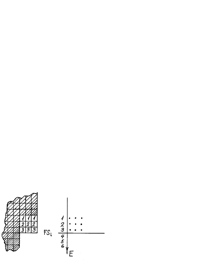
Figure 5: In the figure on the left, we use as an example the case of $N_{i}=3$ columns that have the same length. This is one of perhaps many occurences of $N_{j}$ columns having the same length in the ground state Young tableau for the Universe. The $N_{j}$ columns of the same length define an effective Fermi surfaces $FS_{j}$ at the terminius of these $N_{j}$ columns. $N_{j}$ is expected to be small, perhaps 2 or 3, because column endings are generically widely separated but can be bunched into small clusters because of the HOMO-LUMO gap effect. Only the states above the $N$ coincident column endings need be considered and of these, only those near the column endings. The unimportant part of the Young tableau is cross-hatched in the figure. In the Figure we consider a Fermi sea that is “3 states deep”. Using a deeper Fermi sea has no effect on the ensuing arguments.

The situation of Figure 5 is imagined to be the $i$th occurence of perhaps a whole set of similar occurences $\{FS_{j},N_{j}\}$ where $N_{j}$ columns of equal length end at an effective Fermi surface $FS_{j}$. Each of these $FS_{j}$ corresponds to a particle species $j$ for which the poor physicist has access to excitations near $FS_{j}$ but not to excitations that would allow him to bring particles from $FS_{i}$ to $FS_{j}$ ($i\neq j$). Being able to do this would reveal to him that the $i$th and $j$th particles were really the same (by the arguments of section 3).

We have already argued that the generic stucture of Young diagrams indicates that the $FS_{j}$ are expected to be energetically widely separated and that the $N_{j}=1$ is expected. Only upon invoking the HOMO-LUMO Gap Effect can we argue that some $N_{j}$ can be expected to be slightly larger than 1 (e.g., 2 or 3).

In Figure 5 the integers 1,2,3 label the different single partice states in order of increasing energy. This is the ground state and corresponds to the “clean” Dirac sea (i.e., no holes and no excitations of single particle states lying above the Fermi surface $FS_{i}$). The state 1 is occupied by 3 particles. The same is true for states 2 and 3 as seen in the part of the total Young tableau of Figure 5 that is labelled. The labelling is in accord with that for a standard Young tableau: a standard Young Tabeaux has labels that never decrease in in going from left to right in any row and labels that increase steadily in value in going from the top to the bottom of any column. A Young frame is a tabeau with labels removed; i.e., a Young frame consists of rows (and also columns of course) of plaquettes without labels in them. A Young frame and Young diagram are the same thing and we have used these two terms interchangeably.

Now let us consider an excited configuration corresponding to the creation of $n$ holes and the occupation by $n$ particles of single particle states lying above the Fermi surface $FS_{i}$. Let us use $n=3$ as an example. An excited configration is specified by telling how many of the $n$ holes are in each Dirac Sea state and how many of the $n$ excited particles are in each state above the Fermi Sea $FS_{i}$. For brevity we refer to such a specification as a given “filling” corresponding to an excited configuration. For $n=3$ an example of an excited configuration “filling” is as in Figure 6b. There are of course also many other possible excited configuraion “fillings” for $n=3$ hole/excited-particle pairs. In Figure 6a we show the (unique) ground state “filling”. The number of holes in a state in the excited configuration “filling” is obtained by comparing the number of particles in that state in the ground state “filling” and in the excited configuration “filling”.

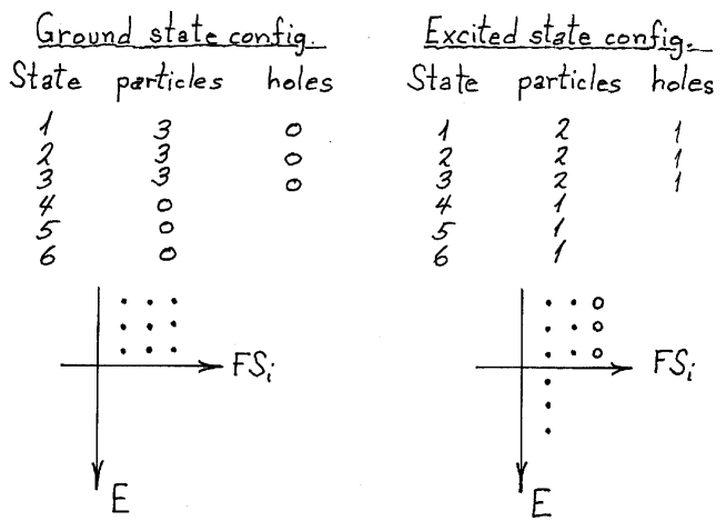
Figure 6: In Figure 6a (on the left) the ground state filling is shown. There are $N=3$ particles i state $1$, $N=3$ particles in state $2$ and $N=3$ particles in state $3$. $N$ is the number of (equal length) columns that all end at the effective Fermi surface labelled “$FS_{i}$. In Figure 6b (to the right) we show the $n=3$ excited state configuration that we want to consider: there are $n=3$ different excited states each occupied by one particle and the $n=3$ Fermi sea states 1,2 and 3 are each occupied by one hole.

We want now to construct the set of standard Young tabeaux consistent with the given “filling” We shall refer to these as “f-allowed standard Young tableaux. We continue to use the filling of Figure 6 with $n=3$ as an example. The possible f-allowed standard Young tableaux for the filling of Figure 6 are depicted in the left column of Figure 7. We see that there are 6 f-allowed standard Young tableaux for the “filling” of Figure 6. These f-allowed standard Young tableaux are numbered from 1 to 6 for future reference.

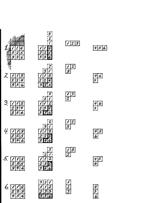
Figure 7: Seen in the left column are the f-allowed standard Young tableaux (numbered 1 to 6) for the “filling” corresponding to the configuration with $n=3$ holes and $n=3$ excited particles at the terminus of $N=3$ columns of equal length as shown in Figure 6 In the next column, the (non-standard) tablaux for the $n=3$ “holes and $n=3$ “excited particles” are identified respectively by broken-line frames drawn above the f-allowed standard Young tableau in question and a bold-line frame within the f-allowed standard Young tableau in question. In the third and fourth columns, the (non-standard) respectively “hole”, and “excited particle” tableaux identified in the second column are rendered in standard Young tableau form.

The aim, using our example with $N=3$ and $n=3$, is, for each f-allowed standard Young tableaux in the allowed set (corresponding to the given “filling”), to illustrate a correspondence between such an f-allowed standard Young tableaux and a pair of standard Young tableaux (each consisting of $n=3$ plaquettes) where one member of the pair is for the $n$ holes created in the given “filling” (i.e., Figure 6 in which $n=3$) and the other member of the pair is for the excited particles of the “filling” (i.e., the $n=3$ particles occupying states above the Fermi sea $FS_{i}$). Let us refer to these pair members as the “hole”standard Young tableau and “excited particle”standard Young tableau respectively. So in the sequel, we shall be referring to standard Young tableaux of three types: f-allowed standard Young tableaux, “hole” standard Young tableaux and “excited particle standard Young tableaux. We now proceed to identify the “hole/(excited)particle” pair of standard Young tableaux corresponding to each f-allowed standard Young tableau.

In the next column of Figure 7, the f-allowed standard Young tableau are drawn again but this time we, for each f-allowed standard Young tableau, identify an (as yet non-standard) “excited particle” tableau that is enclosed by a bold line frame and a (as yet non-standard) “hole” tableau that is drawn with broken lines above the relevant f-allowed standard Young tableau. Each column of the “hole” tableau is labelled by the missing Dirac sea states in that column relative to the ground state “filling”. We use the rule that the label of the missing state of largest negative energy is put in the bottom plaquette of the broken-line column, the next to largest negative energy missing state in the next to bottom plaquette, etc. All the “hole” and all the “excited particle” tableaux consist of $n=3$ plaquettes since the excited configuration of Figure 6 that we are using as an examnpe has $n=3$ excited particles and $n=3$ holes.

Having now identified the (as yet non-standard) “hole” and “excited particle” tableau pair corresponding to each allowed standard Young Tableau, we put these non-standard “hole” and “excited particle” tableax into the standard Young tableau form as follows. For the “hole” non-standard tableaux, we reflect the (labelled) plaquettes about the “SW to NE” diagonal. This yields the desired “hole” standard Young tableaux as seen in column 3 of Figure 7. For the “excited particle” non-standard tableaux, we reflect the (labelled) plaquettes about the “SW to NE” diagonal and reverse the order of the labels to get the standard Young tabeaux form for the “excited particle” tableaux (shown in Column 4 of Figure 7).

So far we have - for each f-allowed standard form Young tableau belonging to the set of f-allowed standard Young tableaux for the given “filling” - found a recipe for being able to see that there is a one-to-one correspondence between each f-allowed standard Young tableau and a pair of standard $n=3$ Young tableaux where the pair consists of a standard “hole” Young tableau and a standard “excited particle” Young tableau. These are shown in Columns 3 and 4 respectively og Figure 7.

We now want to use this one-to-one correspondence in conjunction with well known knowledge about the total number of standard Young tableaux havng $n$ plaquettes ($n=3$ in our example) to tell us the total number of f-allowed standard Young tableax allowed by a given “filling”. But first let us finish the special case of our example with $N=n=3$.

Observe now that there are 3 different Young frames occuring in Columns 3 and 4 of Figure 7. One type - call it Young frame 1 - has the $n=3$ plaquettes all in one row. Another type - call it Young frame 2 - has two plaquettes in the first row and one plaquette in the second row. The third frame type - call it Young frame 3 - has all $n=3$ plaquettes in the same column.

The f-allowed standard Young tableau “number 1” in the first column of Figure 7 is labelled by one standard Young tableau for the “holes” and one standard Young tableau for the “excited particles” both of which are of Young frame type 1 and corresponds by convention to the fully symmetrized (singlet) representation of the symmetric group $S_{3}$ (all plaquettes in a single row). We denote by the symbol $f_{1}$ the number of standard Young tableaux that have the Young frame 1. For the fully symmetrized Young frame we have $f_{1}=1$ (this is also true for any $n$). The f-allowed standard Young tableau “number 6” in the first column of Figure 7 is labelled in an analogous fashion by a “hole” standard Young tableau and a “excited particle” standard Young tableau both of Young frame type 3 corresponding to the “fully antisymmetrized” (singlet) representation of the symmetric group $S_{3}$ (all plaquettes in a single column). We denote by the symbol $f_{3}$ the number of standard Young tableaux that have the Young frame 3. For the fully antisymmetrized Young frame we have $f_{3}=1$ (this is also true for any $n$).

Note now that the “hole” standard Young tableaux and the “excited particle” standard Young tableaux identified with the f-allowed standard Young tableaux numbers 2,3,4 and 5 in the left column of Figure 7 all have the type 2 Young frame - namely the Young frame which corresponds to the mixed symmetry case (with two plaquettes in the first row and one plaquette in the second row). Denote by the symbol $f_{2}$ the number of standard Young tableaux having the type 2 Young frame. For both the “hole” and the “excited particle” standard Young tableax we see that $f_{2}=2$ correponding to the two doublet representations of the group $S_{3}$. Each of the f-allowed standard Young tableaux 2,3,4 and 5 in Figure 7 is in a one-to-one correspondence with a pair of standard Young tableaux namely one of the $f_{2,``hole^{\prime\prime}}=2$ possible “hole” standard Young tableaux and one of the $f_{2,``excited\;part.^{\prime\prime}}=2$ possible “excited particle” standard Young tableaux. For the “hole” and the “excited particle” standard Young tableaux of Young frame type 2, this scheme provides a total of $f_{2,``hole^{\prime\prime}}\cdot f_{2,``excited\;part.^{\prime\prime}}$ = $2^{2}$ labels that have a one-to-one correspondence to the four f-allowed standard Young tableaux with numbers 2,3,4 and 5 in Figure 7.

In our example with $n=3$ plaquettes, the total number of labels provided by the two sets of standard Young tableaux (one set for “holes” and one set for “excited particles”) is

$$f_{1}^{2}+f_{2}^{2}+f_{3}^{2}=1^{2}+2^{2}+1^{2}=6=3!$$ (117)

Due to the one-to-one correspondence between f-allowed standard Young tableaux for the given “filling” and the 3! labels that we get using the “hole” and “excited particle” standard Young tableaux, we conclude that the number of standard Young tablaeux allowed by the given “filling” is also $n!=3!$.

We now use a couple of theoremsber from group theory about Young frames and standard Young tableaux to establish the general validity of the result obtained in our example with $n=3$.

Theorem 1

The number of standard Young tableaux which belongs to the Young frame with row lengths (measured in plaquettes) $m_{1},m_{2},\cdots,m_{r}$ $(m_{1}+m_{2}+\cdots+m_{r}=n)$ with $n$ being the total number of plaquettes is

$$f=n!\frac{\prod_{l<k}(l_{i}-l_{k})}{l_{1}!l_{2}!\cdots l_{r}!}$$ (118)

where $l_{1}=m_{1}+r-1,l_{2}=m_{2}+r-2,\cdots,l_{r}=m_{r}$

Theorem 2

If the index $j$ enumerates the different Young frames that all have $n$ plaquettes, then the total number of standard Young tableaux corresponding to all Young frames made up of $n$ plaquettes is given by

$$\sum_{j}f^{2}_{j}=n!$$ (119)

Using these theorems in conjunction with the one-to-one correspondence between f-allowed standard Young tableaux for a $n$ hole/(excited)particle configuration and all the $\sum_{j}f^{2}_{j}=n!$ possible labellings that are possible by using all possible standard Young tableaux having $n$ plaquettes, we conclude that there are $n!$ allowed standard Young tableaux for a configuration with $n$ excited particles (and $n$ holes). In the event that $N<n$, some of the standard Young tableaux are not realizable (i.e., those containing row lengths greater than $N$ in which case the number of allowed standard Young tableaux is less than $n!$).

32.2 Counting the number of $SU(N)$ singlets that can be obtained by contracting $n$ particles and $n$ anti-particles each having $N$ colors

Consider now $n$ particles $p_{a}$ and $n$ anti-particles $\overline{p^{a}}$ where the index $a$ labels $N$ possible colors. We ask how many $SU(N)$ singlets are obtainable by contracting the $n$ particles with the the $n$ anti-particles. It is rather easy to see that (for $n\leq N$) the number of singlets that can be produced in this way is $n!$.

32.3 Postulating SU(N) symmetry

The number of $SU(N)$ singlets that result from contracting $n$ particles that can have $N$ different “colors” with $n$ anti-particles that can have $N$ different “(anti) colors” is $n!$ (for $n\leq N$). The number of f-allowed standard Young tableaux for the excitation of $n$ particles to states lying above an effective Fermi surface at the terminus of $N$ column of equal length somewhere in a Young tableau for “the Universe” is also equal to $n!$ (for $n\leq N$).

It is left as an exercise for the reader to show that an equality also holds for $N<n$ albeit for a number less than $n!$.

We therefore postulate that the particles near the effective Fermi surface at the terminus of $N$ columns of equal length fall into $SU(N)$ multiplets and have therefore $SU(N)$ symmetry. Because such particles are totally confined (i.e. only realized as colorless singlets), our postulate of $SU(N)$ symmetry can never be challenged: singlets always rotate into singlets. We can postulate $SU(N)$ symmetry because color is globally zero (a singlet). Note that since we have singlets, or rather only one state of the theory for each representation, the color rotation symmetry does not predict any (physical) degeneracies.

33 Conclusion

The basic idea is that when the poor physicist only sees a certain very small number of the (linear superpositions of) states obtained from each other by permutation of the genuinely individual (at Planck scale) particles, he will most likely interprete the particles that he observes as a poor physicist as being identical. If he only sees one single state for each “filling” in an excited configuration, he can consistently interprete the particles as being either simple bosons or simple fermions.

But if the number of f-allowed states per “filling” becomes larger than one, the picture of what a poor physicist sees becomes slightly more sophisticated. We have found that, in the case of the Young frame with $N$ columns of the same length all ending at an effective Fermi surface, one gets the right number of states by pretending that the (fermions say) are $N$-plets under an $SU(N)$ symmetry with the restriction that only singlets are allowed (a kind of confinement postulate). The poor physicist will encounter no contradiction in assuming such an $SU(N)$ symmetry because, with only singlet states allowed in the $SU(N)$ symmetry, the assumption will have no predictive power. Any Hamiltonian is allowed.

In the third section we assume a Planck scale universe that, in the spirit of Random Dynamics, consists of particles that are all different (individual). By further assuming that the Hamiltonian contains very strong particle exchange forces, we show in the context of a very simple model (i.e., a $n$=2 particle universe), that these particles are perceived as being either identical fermions or identical bosons at energies accessible to experiment provided that, in some cases (when more than one Young frame column have the same length) we include a “color description” to take into account the degrees of freedom due to a low energy vestige of the fundamental individuality at the Planck scale.

Again inspired by Random Dynamics, we examine in the fourth section the generic structure of a Young tableau for an $n$-particle universe. The characteristic feature is that only one column of a typical Young tableau ends at a given energy and that adjacent (single) column endings are widely separated in energy. At low energies and in the case of fermions, these column endings function as energetically isolated Fermi surfaces. Inasmuch as the only hole excitations accessible at low energies must lie very near these isolated Fermi surfaces, the “poor physicist” perceives the fermions at each surface as a different species. So even for fermions that are effectively identical as a result of the exchange force mechanism described in section 3, the energetically poor physicist can not afford to make the comparison needed to establish this because he does not have access to hole excitations so deep within the Fermi sea so as to be near an adjacent Fermi surface (i.e., an adjacent column ending).

In section 5 we consider the way in which the HOMO-LUMO gap effect can be expected to modify the spectrum of Fermi surfaces corresponding to the generic Young diagram for a $n$-particle universe as described in section 4. The HOMO-LUMO gap effect, which is seen in e.g. the Jahn-Teller effect, is stated in a more general context (e.g., that of Random Dynamics) as the energetically favourable adjustment of “background” variables that results in the depletion of energy level density at a Fermi surface. This has the effect that some small number $N$, 2 or 3 perhaps, of not too widely separated column endings get pushed together at one effective Fermi surface (i.e., $N$ columns of a total Young tableau of the Universe assume equal lengths).

In section 5 we argue that particles in states near the $N$ column endings of the same length can be claimed to be $SU(N)$ multiplets. The claim of having $SU(N)$ symmetry cannot be challenged because the $SU(N)$ symmetry is realized globally as (confined) $SU(N)$ singlets. This opens the door for future work that may reveal that this globally colorless $SU(N)$ symmetry can turn out to be manifested locally as non-trivial $SU(N)$ representations with the possibility of interactions through e.g. locally manifested $SU(N)$ gauge fields.

*About Number of Families D. Lukman¹, A. Kleppe² and N.S. Mankoč Borštnik^1,3

34 Introductions

The Standard electroweak model gives no explanation for either the number of spinor families (fermions) or for spinor masses (masses of quarks and leptons). According to the Standard electroweak model the families of spinors manifest anomaly freedom (as also the families of antispinors do) as well as gauge invariance. Each family consists of at first massless left handed weak charged doublets and right handed weak chargeless singlets

$$\left[\begin{array}[]{rcl}&\nu_{e}&\\ &e&\end{array}\right]_{L}{\hskip 8.53581pt}{\hskip 8.53581pt}\left[\begin{array}[]{rcl}&u&\\ &d&\end{array}\right]_{L}{\hskip 8.53581pt}\begin{array}[]{rcl}&(\nu_{R})&\\ &e_{R}&\end{array}{\hskip 8.53581pt}{\hskip 8.53581pt}\begin{array}[]{rcl}&u_{R}&\\ &d_{R}&\end{array}.$$

(We put the right handed neutrino into parentheses, since the Standard model does not assume its existence. One of the reasons for that is that a right handed neutrino would have zero as value for all the charges of the Standard model. If it exists, it could interact only through the gravitational interaction.) Spinors acquire masses due to Yukawa couplings (this is done by an assumption), which is a kind of an interaction between weak charge doublets of Higgs scalars (with respect to the group $SO(1,3)$) and massless spinors. All the current data are in agreement with the assumption of only three families. In ref.okun , however, the authors are analyzing possible masses of a fourth family, which do not contradict the experimental data.

We present bellow the experimental values for the masses of the three known families of spinors as well as the masses of a possible fourth family suggested in ref.okun ) as values, which do not contradict the present experimental data.

$$\begin{array}[]{rcl}&&m_{u_{i}}=0.004{\hskip 2.84526pt}GeV,{\hskip 2.84526pt}1.4{\hskip 2.84526pt}GeV,{\hskip 2.84526pt}180{\hskip 2.84526pt}GeV,{\hskip 2.84526pt}285(215){\hskip 2.84526pt}GeV\\ &&m_{d_{i}}=0.009{\hskip 2.84526pt}GeV,{\hskip 2.84526pt}0.2{\hskip 2.84526pt}GeV,{\hskip 2.84526pt}6.3{\hskip 2.84526pt}GeV,{\hskip 2.84526pt}215(285){\hskip 2.84526pt}GeV\\ &&m_{e_{i}}=0.0005{\hskip 2.84526pt}GeV,{\hskip 2.84526pt}0.105{\hskip 2.84526pt}GeV,{\hskip 2.84526pt}1.78{\hskip 2.84526pt}GeV,{\hskip 2.84526pt}100{\hskip 2.84526pt}GeV,\\ }{}{\hfil&&m_{\nu_{i}}=10^{-11}GeV,{\hskip 2.84526pt}10^{-9}GeV,{\hskip 2.84526pt}10^{-8}GeV,{\hskip 2.84526pt}50{\hskip 2.84526pt}GeV.\end{array}$$

The two values in parentheses represent two possibilities for the masses of the fourth generation, suggested by ref.okun , both being in agreement with the experimental data. Values for the neutrino masses of three generations are just guessed in agreement with the experimental data, since the experimental data suggest the square of mass differences among families and not really the masses.

There are many proposals in the literaturebabu ; jarl ; gk ; gm for fermions, which could occur in addition to the known three generations. The most natural and accordingly the most attractive is to our understanding the idea for the fourth replication of just the three known families, with high enough masses, ”allowed” by the ref. (okun ) and small enough mixing matrix elements connecting a possible fourth family with the known three.

Following the approach of one of usnorma93fam ; norma2001 ; pikaholgernorma2002 , we discuss in this contribution the results of the mechanism, which gives the families of quarks and leptons, as well as the Yukawa couplings. The details of the approach can be found in ref.pikaholgernorma2002 . We argue for four generations of quarks and leptons.

35 Approach unifying spins and charges

The approach of one of usnorma93fam ; norma2001 ; pikaholgernorma2002 , unifying spins and charges, is offering mechanisms for both: the appearance of families and accordingly also for the number of families, as well as for interactions which manifest as the Yukawa couplings. The approach assumes the unified internal space of not only all the charges but also of the spins within the group $SO(1,13)$. All spinors and antispinors of one family of the Standard model appear in this approach as just one Weyl spinor of the group $SO(1,13)$ (with right handed weak chargeless neutrino and left handed weak chargeless antineutrino included).

Analyzing the properties of the Weyl spinor with respect to the subgroups $SO(1,3)$, $SU(3),$ $SU(2)$ and the two $U(1)$’s of the group $SO(1,13)$ (the rank of $SO(1,13)$ is $7$ as it is also the sum of the ranks of $SO(1,3),SU(3),SU(2)$ and the two $U(1)$), one easily seespikaholgernorma2002 that there are left handed spinors with respect to the subgroup $SO(1,3)$, which are the $SU(2)$ doublets and either singlets (leptons) or triplets (quarks) with respect to $SU(3)$ and right handed (with respect to $SO(1,3)$) $SU(2)$ singlets, which again are either singlets or triplets with respect to $SU(3)$ within one Weyl spinor (one fundamental irreducible representation). Within the same Weyl spinor one finds also the right handed (with respect to $SO(1,3)$) $SU(2)$ doublets which are antitriplets or antisinglets with respect to $SU(3)$ and left handed (with respect to $SO(1,3)$) $SU(2)$ singlets, which are again antitriplets and antisinglets with respect to $SU(3)$. The Weyl multiplet of $SO(1,13)$ has namely $2^{d/2-1}$ members, which is $2^{6}=64$ (that is $16$ spinors with spin up and down and $16$ antispinors with spin up and down), which means that the family includes also the right handed weak chargeless spinors called right handed neutrinos and the antifamily includes the left handed weak chargeless antineutrino, the antiparticle of the right handed neutrino. Since there are two $U(1)$ charges in $SO(1,13)$ besides $SO(1,3)$ spins and $SU(3)$ and $SU(2)$ charges, the right handed neutrino and the left handed antineutrino carry a nonzero (one of the two) hyper charge.

In the approach unifying spins and charges there are two kinds of generators of the Lorentz transformations and accordingly of the corresponding spin connectionspikaholgernorma2002 , which cause transitions between right handed weak chargeless singlets and left handed weak charged doublets. One kind of generators makes transitions within a family, another kind makes transitions among the families, both together manifesting accordingly the properties of the Yukawa couplings and the Higgs doublets. In this contribution we shall not explain how the Lagrange density for spinors in $d=1+13$ might split in four dimensional subspace into the Lagrange density with the usual covariant derivative manifesting the interaction with the known gauge fields and the part manifesting the mass matrices. The reader can find the explanation in ref.pikaholgernorma2002 . We shall only summarize the results, representing them in mass matrices. We shall further assume that the elements are real numbers in order to study a general behavior of families.

The approach unifying spins and charges suggests even number of families, the smallest number is equal to four

$$\left[\begin{array}[]{rcl}&\nu_{i}&\\ &e_{i}&\end{array}\right]_{L}{\hskip 8.53581pt}{\hskip 8.53581pt}\left[\begin{array}[]{rcl}&u_{i}&\\ &d_{i}&\end{array}\right]_{L}{\hskip 8.53581pt}\begin{array}[]{rcl}&\nu_{iR}&\\ &e_{iR}&\end{array}{\hskip 8.53581pt}{\hskip 8.53581pt}\begin{array}[]{rcl}&u_{iR}&\\ &d_{iR}&\end{array},$$

with $i\in\{1,2,3,4\}$, which is the family number. The approach unifying spins and charges suggests, if we assume real matrix elements (we shall do that for simplicity-just to study general features of mass matrices), the following structure of the Yukawa couplingspikaholgernorma2002

$${M_{4}}=\left(\begin{array}[]{rcl}A_{a}&B_{a}{\hskip 11.38109pt}C_{a}{\hskip 11.38109pt}D_{a}\\ B_{a}&A_{a}{\hskip 11.38109pt}D_{a}{\hskip 11.38109pt}C_{a}\\ C_{a}&D_{a}{\hskip 11.38109pt}A_{a}{\hskip 11.38109pt}B_{a}\\ D_{a}&C_{a}{\hskip 11.38109pt}B_{a}{\hskip 11.38109pt}A_{a}\end{array}\right),$$

with $a$ which stays for $u,d,\nu,e.$ The matrix has the symmetry structure

$$\left(\begin{array}[]{rcl}X&Y\\ Y&X\\ \end{array}\right).$$

Diagonalizing this mass matrix we obtain the eigenvalues

$$\lambda_{a_{1}} = (A_{a}-B_{a})-(C_{a}-D_{a}),$$

$$\lambda_{a_{2}} = (A_{a}-B_{a})+(C_{a}-D_{a}),$$

$$\lambda_{a_{3}} = (A_{a}+B_{a})-(C_{a}-D_{a}),$$

$$\lambda_{a_{4}} = (A_{a}+B_{a})+(C_{a}+D_{a}),$$ (126)

the masses, which should be equalized with the experimental values $m_{a_{i}}$ of Eq.(34), with $a_{i}$, which stays for the members $u_{i},d_{i},\nu_{i},e_{i}$ of the $i$-th family.

One can express $A_{a},B_{a},C_{a},D_{a}$ in terms of masses as follows

$$A_{a} = \{(m_{a_{4}}+m_{a_{3}})+(m_{a_{2}}+m_{a_{1}})\}/4$$

$$B_{a} = \{(m_{a_{4}}+m_{a_{3}})-(m_{a_{2}}+m_{a_{1}})\}/4$$

$$C_{a} = \{(m_{a_{4}}-m_{a_{3}})+(m_{a_{2}}-m_{a_{1}})\}/4$$

$$D_{a} = \{(m_{a_{4}}-m_{a_{3}})-(m_{a_{2}}-m_{a_{1}})\}/4.$$ (127)

Taking into account Eq.(34) we find

$$\begin{array}[]{cccc}A_{u}=116.6&B_{u}=115.899&C_{u}=26.599&D_{u}=25.901\\ (A_{u}^{\prime}=99.101&B_{u}^{\prime}=98.399&C_{u}^{\prime}=9.099&D_{u}^{\prime}=8.401)\\ A_{d}=55.377&B_{d}=55.2728&C_{d}=52.223&D_{d}=52.127\\ (A_{d}^{\prime}=72.877&B_{d}^{\prime}=72.773&C_{d}^{\prime}=69.723&D_{d}^{\prime}=69.627)\\ A_{e}=25.471&B_{e}=25.419&C_{e}=24.581&D_{e}=24.529\\ A_{\nu}=12.5&B_{\nu}=12.5&C_{\nu}=12.5&D_{\nu}=12.5,\end{array}$$ (128)

with all the values in $GeV.$ The values in parentheses correspond to two possibilities for the allowed masses of a possible fourth family.

The ”democratic” matrix with $A_{a}=B_{a}=C_{a}=D_{a}$ would lead, as we can immediately see from Eq.(126), to $\lambda_{a_{1}}=\lambda_{a_{2}}=\lambda_{a_{3}}=0,\;\lambda_{a_{4}}=4A_{a}\;$. All the matrix elements besides the diagonal one equal to zero means $\lambda_{a_{i}}=A_{a},\;i=1,2,3,4.\;$ Since the masses of the fourth family are for all the quarks and the leptons pretty higher than of the other three families, we expect that the mass matrices are closer to the ”democratic” one than to the diagonal one, what indeed is happening. One also can notice that if $C=D=0$ the two by diagonal matrices require the doubling of the eigenvalues $\lambda_{a_{i}}$ that is $\lambda_{a_{1}}=\lambda_{a_{2}}=(A-B),\;\lambda_{a_{3}}=\lambda_{a_{4}}=(A+B)$.

To understand better what more than four families can mean (in the proposed approach of one of us unifying spins and charges the number of families is equal to $4^{k}$) let us look at the case with eight families, again assuming that matrix elements are real numbers. The approach of one of us suggests the matrices

$${M}_{8}=\left(\begin{array}[]{rcl}A_{a}&B_{a}{\hskip 11.38109pt}C_{a}{\hskip 11.38109pt}D_{a}{\hskip 11.38109pt}E_{a}{\hskip 11.38109pt}F_{a}{\hskip 11.38109pt}G_{a}{\hskip 11.38109pt}H_{a}\\ B_{a}&A_{a}{\hskip 11.38109pt}D_{a}{\hskip 11.38109pt}C_{a}{\hskip 11.38109pt}F_{a}{\hskip 11.38109pt}E_{a}{\hskip 11.38109pt}H_{a}{\hskip 11.38109pt}G_{a}\\ C_{a}&D_{a}{\hskip 11.38109pt}A_{a}{\hskip 11.38109pt}B_{a}{\hskip 11.38109pt}G_{a}{\hskip 11.38109pt}H_{a}{\hskip 11.38109pt}E_{a}{\hskip 11.38109pt}F_{a}\\ D_{a}&C_{a}{\hskip 11.38109pt}B_{a}{\hskip 11.38109pt}A_{a}{\hskip 11.38109pt}H_{a}{\hskip 11.38109pt}G_{a}{\hskip 11.38109pt}F_{a}{\hskip 11.38109pt}E_{a}\\ E_{a}&F_{a}{\hskip 11.38109pt}G_{a}{\hskip 11.38109pt}H_{a}{\hskip 11.38109pt}A_{a}{\hskip 11.38109pt}B_{a}{\hskip 11.38109pt}C_{a}{\hskip 11.38109pt}D_{a}\\ F_{a}&E_{a}{\hskip 11.38109pt}H_{a}{\hskip 11.38109pt}G_{a}{\hskip 11.38109pt}B_{a}{\hskip 11.38109pt}A_{a}{\hskip 11.38109pt}D_{a}{\hskip 11.38109pt}C_{a}\\ G_{a}&H_{a}{\hskip 11.38109pt}E_{a}{\hskip 11.38109pt}F_{a}{\hskip 11.38109pt}C_{a}{\hskip 11.38109pt}D_{a}{\hskip 11.38109pt}A_{a}{\hskip 11.38109pt}B_{a}\\ H_{a}&G_{a}{\hskip 11.38109pt}F_{a}{\hskip 11.38109pt}E_{a}{\hskip 11.38109pt}D_{a}{\hskip 11.38109pt}C_{a}{\hskip 11.38109pt}B_{a}{\hskip 11.38109pt}A_{a}\end{array}\right).$$

Again $a$ stays for the members of a family $u,d,\nu,e$. These matrices have the symmetry structure of Eq.(35), as was already the symmetry structure of the case with fourth family. Now each of block $X$ and $Y$ itself has the two by two structure of Eq.(35). One then accordingly easily finds the corresponding eigenvalues

$$\lambda_{a_{1}} = \{(A_{a}-B_{a})-(C_{a}-D_{a})\}-\{(E_{a}-F_{a})-(G_{a}-H_{a})\}$$

$$\lambda_{a_{2}} = \{(A_{a}-B_{a})-(C_{a}-D_{a})\}+\{(E_{a}-F_{a})-(G_{a}-H_{a})\}$$

$$\lambda_{a_{3}} = \{(A_{a}-B_{a})+(C_{a}-D_{a})\}-\{(E_{a}-F_{a})+(G_{a}-H_{a})\}$$

$$\lambda_{a_{4}} = \{(A_{a}-B_{a})+(C_{a}-D_{a})\}+\{(E_{a}-F_{a})+(G_{a}-H_{a})\}$$

$$\lambda_{a_{5}} = \{(A_{a}+B_{a})-(C_{a}+D_{a})\}-\{(E_{a}+F_{a})-(G_{a}+H_{a})\}$$

$$\lambda_{a_{6}} = \{(A_{a}+B_{a})-(C_{a}+D_{a})\}+\{(E_{a}+F_{a})-(G_{a}+H_{a})\}$$

$$\lambda_{a_{7}} = \{(A_{a}+B_{a})+(C_{a}+D_{a})\}-\{(E_{a}+F_{a})+(G_{a}+H_{a})\}$$

$$\lambda_{a_{8}} = \{(A_{a}+B_{a})+(C_{a}+D_{a})\}+\{(E_{a}+F_{a})+(G_{a}+H_{a})\}.$$ (129)

If we now call ${\cal A}_{a}=(A_{a}-B_{a}),\;{\cal B}_{a}=(C_{a}-D_{a}),\;{\cal C}_{a}=(E_{a}-F_{a}),\;{\cal D}_{a}=(G_{a}-H_{a}),\;$ then the values of Eq.(127) for $A,B,C,D$ have to be identified with ${\cal A},{\cal B},{\cal C},{\cal D}\;$, correspondingly and fitted accordingly with the masses of Eq.(34). One easily sees that then the last four values for $\lambda_{a_{i}}$ can allways be chosen to be as large as needed in order that the four additional families can not be experimentaly seen.

This kind of doubling the number of families can be continued. Due to (by the approach of unifying spins and charges) suggested symmetry of the mass matrix (Eq.(35), this symmetry keeps when ever we double the number of families) the eigenvalues $\lambda_{a_{i}}$ can easily be found and the lowest four families then identified with the four types of values of Eq.(34) in a way that all the rest of the eigenvalues acquire (very) high masses an can not be seen at present energies. In the next step of doubling ${\cal A}_{a}=\{(A_{a}-B_{a})-(C_{a}-D_{a})\},\;{\cal B}_{a}=\{(E_{a}-F_{a})-(G_{a}-H_{a})\},\;{\cal C}_{a}=\{(I_{a}-J_{a})-(K_{a}-L_{a})\},\;{\cal D}_{a}=\{(M_{a}-N_{a})-(O_{a}-P_{a})\},\;$ with $I,J,K,L,M,N,O,P\;$ the matrix elements of the doubled structure and with the starting symmetry all the time.

36 Conclusions and discussions

Following the approach of one of usnorma93fam ; norma2001 ; pikaholgernorma2002 and the ref.okun we argue in this contribution for an even number of families, in particular for four families, with the fourth family having all the properties, besides the masses, equal to the properties of the known three families.

The approach (unifying spins and charges) is offering a mechanism for not only the appearance of families, which should be an even number, but also for the appearance of the Yukawa couplings and Higgs: It is a spin connection in higher dimensions than four ( that is the gravitational interaction) which in four dimensional subspace might manifest as correct mass terms for (otherwise massless) spinors. This approach has in one $SO(1,13)$ multiplet (one Weyl spinor) just all the quarks and the leptons (the left handed weak charged doublets and the right handed weak chargeless singlets, which are either colour charge triplets - quarks - or colour chargeless singlets-leptons), as well as all the antiquarks and all the antileptons, with right handed weak chargeless neutrinos and the left handed weak chargeless antineutrinos included.

To study properties of mass matrices, we assume that matrix elements, suggested by the approach, are real numbers. Due to the symmetry of the mass matrix (Eq.(35)), suggested by the approach, and due to the assumption of real numbers one then easily finds the eigenvalues of the mass matrices and demonstrate that eigenvalues can agree with the experimental data and the ref.okun . It also turns out that the mass matrix, if fitted to the experimental data, demonstrate the structure, which is pretty close to the ”democratic” matrix.

Since the approach is offering indeed $(2^{2k})$, with $k=1,2,3$, families (with the interaction in higher dimensions and accordingly with the masses of families, which depend on the way how the group $SO(1,13)$ breaks and also on the corresponding running coupling constants) we look for the eigenvalues of matrices of the dimension $(2^{2k})\times(2^{2k})$. We find that there are the differences of the mass matrix elements, which determine the masses of the four lowest families, while the rest of families lie at much higher values.

We intend to study further properties of the mass matrices, suggested by the approach unifying spins and charges. We shall evaluate the mass matrices to predict differences in mass matrices among the members of one family, complexity of matrix elements and others.

37 Acknowledgement

Two of the authors would like to thank the Ministry of Education, Science and Sport of Slovenia for funding the research as well as the Workshop. All the authors would like to thank the participants at the workshop for really stimulating discussions.

*Coupling Constant Unification in Spin-Charge Unifying Model Agreeing With Proton Decay Measurements N. Mankoč Borštnik^1,2 and H. B. Nielsen³

38 Introduction

The $SU(5)$ grand unified theory (GUT) is rather predictive concerning the three fine structure coupling constants in as far as the three invariant Lie subalgebras of the Standard Model suggest that all the three corresponding coupling constants get separated at the same scale. The SUSY-SU(5) coupling predictions of the very unification has much been celebrated. Non-susy $SU(5)$-GUT has already since long nsgut been in disagreement with experimentally determined gauge coupling constants. Since thus $SU(5)$-G.U.T. is in a bad shape so must be $SO(10)$ broken down along the $SU(5)$-route, i.e. with $SU(5)$ as an intermediate step. However, if you break down (say) $SO(10)$-G.U.T. along a non-$SU(5)$ route you can easily get so many parameters that you can avoid predictions independent of further modelling and thus $SO(10)$ should not be considered killedSO10rev .

One obvious way to break down $SO(10)$ is to break it into $SO(4)\times SO(6)$ which as far as the Lie algebra is concerned is equivalent to $SU(2)\times SU(2)\times SU(4)$ which can then be further broken down by breaking the $SU(4)$ down to $SU(3)\times U(1)$, and one of the $SU(2)$’s to $U(1)$. Finally the weak hypercharge of the Standard Model can then be identified with a linear combination of the two $U(1)$, the rest -essentially a $B-L$ charge - being broken.

This breaking pattern is closely related to the breaking pattern suggested in connection with the spin-charge-unifying model put forward by one of us norma92so ; norma93so ; norma01so . In fact this model starts from a $1+13$ dimensional space-time and it contains in principle $SO(10)$ as a subgroup of its $SO(1,13)$ and thus has an underlying $SO(10)$ symmetry that is even gauged in as far as the whole $SO(1,13)$ is supposed to be gauged - really due to gravity in the high dimensional space time. The first breaking - the one at the highest energies - is supposed in this model to be into $SO(1,7)\times SO(6)$ where the $SO(1,7)$ is supposed to contain the Lorentz group in the finally four dimensions also. The part of this $SO(1,7)$ which is purely ordinary gauge transformation - i.e. not involving any relation to the $1+3$ part of space-time dimensions - is an $SO(4)$ subgroup. This model has spin-charge-unification in the sense that for instance the whole $SO(1,13)$ is supposed to include what at the end shall show up as the Lorentz group in the observed $1+3$ dimensions with all the known charges. Concerning the part of the “inner space” meaning spin - which is the main concern of this model - this spin got unified with the charges in the sense that the Lorentz group is united with the gauge transformation group into the $SO(1,13)$.

$$\begin{array}[]{c}\begin{array}[]{c}\underbrace{\begin{array}[]{rrcll}&&\mathrm{SO}(1,13)\\ &&\downarrow\\ &&\mathrm{SO}(1,7)\otimes\mathrm{SO}(6)\\ &\swarrow&&\searrow\\ &\mathrm{SO}(1,7)&&\mathrm{SU}(4)\\ \swarrow&&&\qquad\downarrow\\ \mathrm{SO}(1,3)\otimes\mathrm{SO}(4)&&&\mathrm{SU}(3)\otimes\mathrm{U}(1)\\ \downarrow&&&\qquad\downarrow\\ \mathrm{SO}(1,3)\otimes\mathrm{SU}(2)\otimes\mathrm{U}(1)&&&\mathrm{SU}(3)\otimes\mathrm{U}(1)\\ &&&\\ \end{array}}\\ \mathrm{SO}(1,3)\otimes\mathrm{SU}(2)\otimes\mathrm{U}(1)\otimes\mathrm{SU}(3)\otimes\mathrm{U}(1)\\ \end{array}\\ \downarrow\\ \mathrm{SO}(1,3)\otimes\mathrm{SU}(2)\otimes\mathrm{U}(1)\otimes\mathrm{SU}(3)\\ \end{array}$$

It turns out that in this model, unifying spins and chargesnorma01so ; pikanormaholger2002 , in one $SO(1,7)$ spinor multiplet, a left handed $SU(2)$ doublets together with a right handed $SU(2)$ singlets occur, just as it is needed as an input for the Standard Model.

Apart from the appearance also of the Lorentz group $SO(1,3)$ and some further generators mixing the latter with the gauge group $SO(10)$, this model is really much like the $SO(10)$ model, being broken to the $SO(4)\times SO(6)$ way. It is the purpose of the present article to investigate if relations among the coupling constants in the Standard Model - $\alpha_{1}$, $\alpha_{2}$, and $\alpha_{3}$ - found experimentally as $\alpha_{elm}$, $\alpha_{W}$, and $\alpha_{S}$ could possibly be consistent with such a break down under the restrictions implied by the mentioned model of the spin-charge unification. As a test we also present in this (non SUSY ) model the proton decay time, for which it comes out that it causes no problem.

39 Group $SO(1,13)$ and subgroups $SO(4)\times SU(4)$ breaking to Standard Model group and $U(1)_{B-L}$

If we ignore the geometrical - i.e. Lorentz transformation in $1+3$ related - components in the group $SO(1,7)$ we are just considering the $SO(4)\times SO(6)$ group at the intermediate level. Note, that a priori in breaking $SO(10)$ one can have each of these subgroups $SO(4)$ and $SO(6)$ breaking further themselves at different scales of energy, thus providing parameters to be fitted at these scales. This situation means that we have as the unavoidable predictions mainly the relations between the “contributions” to the (inverse) weak hypercharge gauge coupling squared $\alpha_{1}$ coming from respectively the $SO(6)$ - a contribution unifying with the $SU(3)$ coupling $\alpha_{3}=\alpha_{S}$ - and the $SO(4)$ unifying with the weak isospin coupling $\alpha_{2}=\alpha_{W}$.

40 Normalization of coupling constants

Let us here perform a little trivial calculation of the parametrization of the Standard Model gauge couplings - in terms of those of $SO(4)$ and $SO(6)$ - as they would appear under the assumptions of:

a) the gauge group $SO(4)\times SO(6)$, the subgroup of $SO(10)$ (lying behind the group of $SO(1,13)$) giving rise to respectively $SU(2)\times U(1)_{SO(4)}$ and $SU(3)\times U(1)_{SO(6)}$,

b) and then having the two $U(1)$’s broken into only one in such a way that the surviving $U(1)$ identifies with the Standard Model $U(1)$ as embedded into conventional $SO(10)$ as it could be containing the mentioned group $SO(4)\times SO(6)$.

Before we shall fix the combination of U(1)-charges to be identified with the Standard Model weak hyper-charge we should choose a normalization of the $U(1)$-group couplings for the $U(1)$’s embedded into respectively $SO(4)$ and $SO(6)$ as respectively $U(1)_{SO(4)}\times SU(2)_{SO(4)}\subseteq SO(4)$ and $U(1)_{SO(6)}\times SU(3)_{SO(6)}\subseteq SU(4)=SO(6)$ and we shall do that so that $SO(4)$ and $SO(6)$ symmetry ensure the same coupling for $U(1)_{SO(4)}$ and $SO(4)$ and $SU(2)$ inside it as well as for $U(1)_{SO(6)}$ and $SO(6)$ and $SU(3)$.

To do that we shall first rearrange the generators $S^{ab}$ of the group $SO(10)$ so that they will manifest the subgroups $SO(4)$ and $SO(6)$ structurenorma92so ; norma93so ; norma01so . Making a choice that indices $k\in 1,2,3,4$ belong to the subgroup $SO(4)$ and $h\in 5,6,7,8,9,10$ to the subgroup $SO(6)$, we find the $SU(2)\times SU(2)$ substructure of $SO(4)$ and make a choice that the generators

$$\tau^{11}: = \frac{1}{2}(S^{14}-S^{23}),\quad\tau^{12}:=\frac{1}{2}(S^{13}+S^{24}),\quad\tau^{13}:=\frac{1}{2}(S^{12}-S^{34}),$$

$$\tau^{2}: = \frac{1}{2}(S^{12}+S^{34})=:Q_{U(1),SO(4)}$$ (130)

close the algebra of the group $SU(2)$ and $U(1)$, respectively

$$[\tau^{Ai},\tau^{Bj}]=if^{Aijk}\tau^{Ak}\delta^{AB},$$ (131)

with $f^{1ijk}=\varepsilon^{ijk}$ and $f^{2ijk}=0$, while $\tau^{31}:=\frac{1}{2}(S^{14}+S^{23})$, $\tau^{32}:=\frac{1}{2}(S^{13}-S^{25})$ together with $\tau^{2}$ form the algebra of the group $SU(2)$ as well.

We express the generators of the subgroups $SU(3)$ and $U(1)$ embedded into $SO(6)$ in terms of $S^{ab}$ as follows

$$\tau^{41}: = \frac{1}{2}(S^{58}-S^{67}),\quad\tau^{42}:=\frac{1}{2}(S^{57}+S^{68}),\quad\tau^{43}:=\frac{1}{2}(S^{12}-S^{34}),$$

$$\tau^{44}: = \frac{1}{2}(S^{510}-S^{69}),\quad\tau^{45}:=\frac{1}{2}(S^{59}+S^{610}),\quad\tau^{46}:=\frac{1}{2}(S^{710}-S^{89}),$$

$$\tau^{47}: = \frac{1}{2}(S^{79}+S^{810}),\quad\tau^{48}:=\frac{1}{2\sqrt{3}}(S^{56}+S^{78}-2S^{910})$$

$$\tau^{5}: = (-)\frac{1}{3}(S^{56}+S^{78}+S^{910})/(\sqrt{2/3}),\quad\tau^{\prime 5}=\sqrt{2/3}\cdot\tau^{5}=:Q_{U(1),SO(6)}$$ (132)

with commutation relations defined in Eq.(131) and with $f^{4ijk}$ which are the standard structure constants of the group $SU(3)$, while $f^{5ijk}=0$. We have introduced besides the operator $\tau^{5}$ also the operator $\tau^{\prime 5}$, since the second one plays the role of the operator determining the number of baryons minus the number of leptons

$$(B-L):=2\cdot\tau^{\prime 5}$$ (133)

and in addition, it is also the operator which, together with the operator $\tau^{2}$, defines the operator $Y^{1}$, which corresponds to 1/2 of the hypercharge $y$ appearing in the Standard Model

$$y/2:=Y^{1}=(\tau^{2}+\tau^{\prime 5}).$$ (134)

We also may define accordingly the operator $Y^{2}$ as an additional hypercharge, since $Y^{1}$ and $Y^{2}$ are the two orthogonal charges, while $Y^{1}$ and $(B-L)$ are not

$$Y^{2}=(-\tau^{2}+\tau^{\prime 5}).$$ (135)

The covariant derivative for spinor representations in the model, which starts with $SO(10)$ (in the proposed model it really starts with $SO(1,13)$), is as follows

$$D_{\mu}=\partial_{\mu}-g\frac{1}{2}S^{ab}\omega_{ab\mu},$$ (136)

where $g$ is the coupling constant of the group $SO(10).$

Taking into account only the $SU(2)\times U(1)_{SO(4)}\times SU(3)\times U(1)_{SO(6)}$ substructure of the group $SO(10)$ (or the $SO(1,3)\times SU(2)\times U(1)_{SO(4)}\times SU(3)\times U(1)_{SO(6)}$ substructure of the group $SO(1,13)$) we can write for spinor representations the corresponding covariant derivative (in the case of $SO(1,13)$ this follows, if gravity in the four dimensional subspace is neglected)

$$D_{\mu}=\partial_{\mu}-\frac{g}{\sqrt{2}}\{\tau^{2}A_{\mu}^{2}+\tau^{5}A_{\mu}^{5}+\mathchoice{\mbox{\boldmath$\displaystyle\tau^{1}$}}{\mbox{\boldmath$\textstyle\tau^{1}$}}{\mbox{\boldmath$\scriptstyle\tau^{1}$}}{\mbox{\boldmath$\scriptscriptstyle\tau^{1}$}}\cdot\mathchoice{\mbox{\boldmath$\displaystyle A$}}{\mbox{\boldmath$\textstyle A$}}{\mbox{\boldmath$\scriptstyle A$}}{\mbox{\boldmath$\scriptscriptstyle A$}}_{\mu}^{W}+\mathchoice{\mbox{\boldmath$\displaystyle\tau^{4}$}}{\mbox{\boldmath$\textstyle\tau^{4}$}}{\mbox{\boldmath$\scriptstyle\tau^{4}$}}{\mbox{\boldmath$\scriptscriptstyle\tau^{4}$}}\cdot\mathchoice{\mbox{\boldmath$\displaystyle A$}}{\mbox{\boldmath$\textstyle A$}}{\mbox{\boldmath$\scriptstyle A$}}{\mbox{\boldmath$\scriptscriptstyle A$}}_{\mu}^{S}\}$$ (137)

and the corresponding Lagrange density

$${\cal L}=\bar{\psi}\gamma^{\mu}P_{\mu}\psi$$ (138)

with $P_{\mu}=iD_{\mu}$. The (only one) coupling constant in Eq.(137) is clearly related to the coupling constant in Eq.(136), since fields $A^{Ai}_{\mu}$ are orthonormal superpositions of $\omega_{ab\mu}$. ( We present here two particular examples, which are $A^{11}_{\mu}=(\omega_{14\mu}-\omega_{23\mu})/\sqrt{2}$, and $A^{48}_{\mu}=(\omega_{56\mu}+\omega_{23\mu}-2\omega_{910\mu})/\sqrt{6}$. The rest of the fields $A^{Ai}$, expressed in terms of $\omega_{ab\mu}$, can be found in ref. norma01so with the normalization factor $1/2$ rather than $1/\sqrt{2}$ as here).

We also can write the covariant derivative presented in Eq.(137) in a way, which points out the Standard Model structure of the group $SO(10)$

$$D_{\mu} = \partial_{\mu}-g_{U(1),SO(4)}\;\tau^{2}A_{\mu}^{2}-g_{U(1),SO(6)}\;\tau^{\prime 5}A_{\mu}^{5}$$ (139)

$$-g_{W}\;\mathchoice{\mbox{\boldmath$\displaystyle\tau^{1}$}}{\mbox{\boldmath$\textstyle\tau^{1}$}}{\mbox{\boldmath$\scriptstyle\tau^{1}$}}{\mbox{\boldmath$\scriptscriptstyle\tau^{1}$}}\cdot\mathchoice{\mbox{\boldmath$\displaystyle A$}}{\mbox{\boldmath$\textstyle A$}}{\mbox{\boldmath$\scriptstyle A$}}{\mbox{\boldmath$\scriptscriptstyle A$}}_{\mu}^{W}-g_{S}\;\mathchoice{\mbox{\boldmath$\displaystyle\tau^{4}$}}{\mbox{\boldmath$\textstyle\tau^{4}$}}{\mbox{\boldmath$\scriptstyle\tau^{4}$}}{\mbox{\boldmath$\scriptscriptstyle\tau^{4}$}}\cdot\mathchoice{\mbox{\boldmath$\displaystyle A$}}{\mbox{\boldmath$\textstyle A$}}{\mbox{\boldmath$\scriptstyle A$}}{\mbox{\boldmath$\scriptscriptstyle A$}}_{\mu}^{S},$$

with

$$g_{W}=g_{S}=g/\sqrt{2}=g_{U(1),SO(4)},\;\;g_{U(1),SO(6)}=\sqrt{3/2}\;g_{U(1),SO(4)},$$ (140)

in agreement with Eq.132.

The notation points out that the coupling constants of the two $U(1)$ subgroups belong to the two different starting subgroups, namely to $SO(4)$ and $SO(6)$.

From Eq.(140) it follows that

$$(g_{U(1),SO(6)})^{2}:(g_{U(1),SO(4)})^{2}=3:2.$$ (141)

Introducing the notation

$$\hat{A}^{Ai}:=g_{A}A^{Ai}_{\mu},\quad A=\{1,2,4,5\},i=\{1,n_{a}\},$$ (142)

with $n_{1}=3,n_{2}=1,n_{4}=8,n_{5}=1$, we may write the Lagrange density for the gauge fields

$${\cal L}=-\frac{1}{4(g_{A})^{2}}Tr(\hat{F}^{Ai\mu\nu}\hat{F}^{Ai}_{\mu\nu}),$$ (143)

with summation performed over $A$ and $i$ and with

$$\hat{F}^{Ai}_{\mu\nu}:=g_{A}\tau^{Ai}\;(\;\partial_{\mu}A^{Ai}_{\nu}-\partial_{\nu}A^{Ai}_{\mu}-\;f^{Aijk}A^{Aj}_{\mu}A^{Ak}_{\nu}\;).$$ (144)

We present in Table 5 quantum numbers of one irreducible representation of the subgroup $SO(1,7)$ of the group $(SO(1,13))$. It coincides with one generation of fermions (left handed weak charged doublets and right handed weak chargeless singlets) of the Standard Model. We find them using the technique presented in refs.norma01so ; normaholgertec2002 , since with the help of this technique one easily finds vectors and the corresponding quantum numbers of one generation.

SU(2) doublets

SU(2) singlets

$\tau^{13}$

$\tau^{2}$

$\tau^{\prime 5}$

$Y_{1}$

$Y_{2}$

$\Gamma^{(4)}$

$\tau^{13}$

$\tau^{2}$

$\tau^{\prime 5}$

$Y_{1}$

$Y_{2}$

$\Gamma^{(4)}$

SU(3)

$\tau^{4\;3}\;\;$ =

$u_{i}$

1/2

0

1/6

1/6

1/6

- 1

0

1/2

1/6

2/3

-1/3

1

tri-

$(\frac{1}{2},$ $-\frac{1}{2},\;\;$ $0\;$ )

plets

$\tau^{4\;8}\;\;$ =

$d_{i}$

-1/2

0

1/6

1/6

1/6

-1

0

-1/2

1/6

-1/3

2/3

1

$(\frac{1}{2\sqrt{3}},$ $\frac{1}{2\sqrt{3}},$ $-\frac{1}{\sqrt{3}}$ )

SU(3)

$\tau^{4\;3}=0$

$\nu_{i}$

1/2

0

-1/2

-1/2

-1/2

-1

0

1/2

-1/2

0

-1

1

singlets

$\tau^{4\;8}=0$

$e_{i}$

-1/2

0

-1/2

-1/2

-1/2

-1

0

-1/2

-1/2

-1

0

1

Table 5: Expectation values of the Cartan subalgebra of the group $SU(3)\times U(1)\subset SU(6)$ and of the group $SU(2)\times U(1)\times SO(1,3)\subset SO(1,7)$, following ref.norma01so . We chose the representations to be eigenvectors of the operators $\tau^{13}$ (Eq.130) and $\tau^{2}$ (Eq.130), $\tau^{43}$ and $\tau^{48}$ (Eq.132) and $\tau^{\prime 5}$ (Eq.132) as well as the operator of handedness $\Gamma^{(4)}$ ($\Gamma^{(4)}=\mp 1$, representing left and right handed spinors, respectively). We also present the sum and the difference of the two $U(1)$ operators $\tau^{5}$ and $\tau^{2}$, which are $Y^{1}$ and $Y^{2}$, respectively.

According to the quantum numbers, presented in Table 5 , we easily see that the operators $\tau^{1i}$ of the group $SU(2),$ the operators $\tau^{4i}$ of the group $SU(3)$ and the operators $\tau^{2}$ are normalized so that

$$Tr\{\tau^{Ai}\tau^{Bj}\}=2\delta^{AB}\delta^{ij},$$ (145)

since we find if following Table 5 for, let say, $Tr\{(\tau^{13})^{2}\}=3\cdot(1/2)^{2}+3\cdot(-1/2)^{2}+3\cdot(0)^{2}+3\cdot(0)^{2}+1\cdot(1/2)^{2}+1\cdot(-1/2)^{2}+1\cdot(0)^{2}+1\cdot(0)^{2}=2$, for, let say, $Tr\{(\tau^{48})^{2}\}=4\cdot(1/(2\sqrt{3}))^{2}+4\cdot(1/(2\sqrt{3}))^{2}+4\cdot(-1/\sqrt{3})^{2}+4\cdot(0)^{2}=2$ and for $Tr(\tau^{2})^{2}=3\cdot(0)^{2}+3\cdot(0)^{2}+1\cdot(0)^{2}+1\cdot(0)^{2}+3\cdot(1/2)^{2}+3\cdot(-1/2)^{2}+1\cdot(1/2)^{2}+1\cdot(-1/2)^{2}=2$. While the operator $\tau^{5}$ is also normalized according to Eq.(145) to $2$, the operator $\tau^{\prime 5}$ is normalized instead to $4/3$. We see this, since according to Table 5 we find that $Tr\{(\tau^{\prime 5})^{2}\}=3\cdot(1/6)^{2}+3\cdot(1/6)^{2}+1\cdot(-1/2)^{2}+1\cdot(-1/2)^{2}+3\cdot(1/6)^{2}+3\cdot(1/6)^{2}+1\cdot(-1/2)^{2}+1\cdot(-1/2)^{2}=2\cdot 2/3$. Similarly we find that both $Tr\{(Y^{1})^{2}\}=2\cdot 5/3$ $(Y^{1}=\tau^{2}+\tau^{{}^{\prime}5})$ and $Tr\{(Y^{2})^{2}=2\cdot 5/3,\;(Y^{2}=-\tau^{2}+\tau^{{}^{\prime}5})\}.$ We namely find that $Tr\{(Y^{1})^{2}\}=3\cdot(1/6)^{2}+3\cdot(1/6)^{2}+1\cdot(-1/2)^{2}+1\cdot(-1/2)^{2}+3\cdot(2/3)^{2}+3\cdot(-1/3)^{2}+1\cdot(0)^{2}+1\cdot(-1)^{2}=2\cdot 5/3=Tr\{(Y^{2})^{2}\}$.

41 Breaking of (B-L) gauge symmetry

We recognize, as we said, in the quantum number $Y^{1}=y/2$ the hypercharge of the Standard Model and in $2\tau^{\prime 5}=(B-L)$ the baryon minus lepton quantum number. We could instead of the $(B-L)$ quantum number as well use the quantum number $Y^{2}$ as the additional quantum number to $Y^{1}$ (Eq.(135)). The first one is the sum of the two $U(1)$ generators belonging to the subgroups $SO(6)$ and $SO(4)$, respectively, of the group SO(10), namely ($\tau^{2}+\tau^{\prime 5}$) (Eq.(134)), while $(B-L)=2\tau^{\prime 5}$ and $Y^{2}=(\tau^{2}+\tau^{\prime 5})$ (Eq.(135)).

Let us now come back to the covariant derivative (Eq.(137)) manifesting the Standard Model structure of the group $SO(10)$ and let us assume that there is a Higgs field $\phi_{Y^{2}}$ with the vacuum expectation value much larger than the weak scale, coupling alone to the $Y^{2}$ hypercharge quantum number but not to the $Y^{1}=y/2$ hypercharge [which means that the vacuum expectation value of $Y^{2},$ $<\phi|Y^{2}|\phi>\neq 0$ while $<\phi|y|\phi>=0$] since it would make say $Z^{0}_{\mu}$ too heavy. ( Let us remaind the reader that the quantum numbers of the Standard Model Higgs just agree, up to the spin and accordingly the handedness, with the quantum numbers of a spinorial field, which is ( a left handed) $SU(2)$ doublet and a $SU(3)$ singlet ( Table 5)).

Since

$$\hat{A}^{Y^{2}}_{\mu}=(\hat{A^{5}}_{\mu}-\hat{A^{2}}_{\mu})/\sqrt{2},$$ (146)

with $A^{2}_{\mu}$ and $A^{5}_{\mu}$ defined in Eq.142, at low energy it must be - due to the sea-gull term for the Higgs field $\phi_{Y^{2}}$ ($\phi_{B-L}$)- that

$$\hat{A^{5}}_{\mu}=\hat{A^{2}}_{\mu}.$$ (147)

As long as the relation of Eq.(147) is valid, the only charge among the two abelian charges ($Y^{1}$ and $Y^{2}$), which matters, is $Y^{1}=y/2$. Effectively, $\tau^{\prime 5}=(B-L)/2$ may also be put to zero, so that effectively

$$(\frac{y}{2})_{{\rm effective}}=\frac{1}{2}Q_{U(1),SO(4)},$$ (148)

but with an effective Lagrange density ${\cal L}_{(\frac{y}{2})_{effective}}$

$$({\cal L}_{\frac{y}{2}})_{{\rm effective}}=-\frac{1}{4(g_{U(1),SO(4)})^{2}}\cdot(1+\frac{2}{3})\hat{F}^{U(1),SO(4)}_{\mu\nu}.$$ (149)

Denoting the $Y^{2}$ (the $(B-L)$) gauge breaking scale weak hypercharge coupling by $g^{\prime}=g_{\frac{y}{2}}$, the covariant derivative has the form

$$D_{\mu}=\partial_{\mu}-(y/2)\hat{A^{\prime y}}_{\mu}-\mathchoice{\mbox{\boldmath$\displaystyle\tau^{W}$}}{\mbox{\boldmath$\textstyle\tau^{W}$}}{\mbox{\boldmath$\scriptstyle\tau^{W}$}}{\mbox{\boldmath$\scriptscriptstyle\tau^{W}$}}\cdot\mathchoice{\mbox{\boldmath$\displaystyle\hat{A}_{\mu}^{W}$}}{\mbox{\boldmath$\textstyle\hat{A}_{\mu}^{W}$}}{\mbox{\boldmath$\scriptstyle\hat{A}_{\mu}^{W}$}}{\mbox{\boldmath$\scriptscriptstyle\hat{A}_{\mu}^{W}$}}-\mathchoice{\mbox{\boldmath$\displaystyle\tau^{S}$}}{\mbox{\boldmath$\textstyle\tau^{S}$}}{\mbox{\boldmath$\scriptstyle\tau^{S}$}}{\mbox{\boldmath$\scriptscriptstyle\tau^{S}$}}\cdot\mathchoice{\mbox{\boldmath$\displaystyle\hat{A}_{\mu}^{S}$}}{\mbox{\boldmath$\textstyle\hat{A}_{\mu}^{S}$}}{\mbox{\boldmath$\scriptstyle\hat{A}_{\mu}^{S}$}}{\mbox{\boldmath$\scriptscriptstyle\hat{A}_{\mu}^{S}$}},$$ (150)

with $\tau^{Wi}=\tau^{1i}$, $\tau^{Si}=\tau^{4i}$ and with the correspondingly defined $\hat{A^{\prime}}^{y}_{\mu}=\hat{A^{\prime}}^{Y^{1}}_{\mu},\hat{A}^{Wi}_{\mu}=\hat{A}^{1i}_{\mu},\hat{A}^{Si}_{\mu}=\hat{A}^{4i}_{\mu}$.

Due to the slavery following from equation (147) we have for the $y$-part of the Lagrange density

$${\cal L}_{(y/2)_{effective}} = -\frac{5}{3}\;\frac{1}{4}\;\frac{1}{(g_{U(1),SO(4)})^{2}}Tr(\hat{F}^{U(1),SO(4)\mu\nu}\hat{F}^{U(1),SO(4)}_{\mu\nu})$$ (151)

$$= -\frac{1}{4}\frac{1}{(g^{\prime})^{2}}Tr(\hat{F^{\prime}}^{\mu\nu}\hat{F^{\prime}}_{\mu\nu}),$$

with

$$\frac{1}{(g^{\prime})^{2}}=\frac{1}{(g_{U(1),SO(4)})^{2}}+\frac{1}{(g_{U(1),SO(6)})^{2}}=\frac{5}{3}\frac{1}{(g_{U(1),SO(4)})^{2}}$$ (152)

and accordingly $\hat{A^{\prime}}^{Y^{1}}_{\mu}=g^{\prime}{A^{\prime}}^{Y^{1}}_{\mu}$.

This is just the usual $SU(5)\subset SO(10)$ prediction for the $U(1)$ coupling constant, assuming that the break occurred at the unification scale, the same for $SO(4)$ and $SO(6)$. After the $Y^{2}$ and accordingly the $(B-L)$ is broken, the Standard Model coupling constants further run, leading to the three lines crossing at one point if $SU(5)(\subset SO(10))$ would work

$$\frac{1}{\alpha^{\prime}_{SU(5)}}\dot{=}\frac{3}{5}\frac{1}{\alpha^{\prime}}.$$ (153)

Instead we have

$$\frac{1}{\alpha^{\prime}_{SU(5)}}=\frac{3}{5}(\frac{1}{\alpha_{U(1),SO(4)}}+\frac{1}{\alpha_{U(1),SO(6)}})=\frac{3}{5}\frac{1}{\alpha_{2}}+\frac{2}{5}\frac{1}{\alpha_{3}}.$$ (154)

We present a plot of experimental values of $(\alpha^{\prime})^{-1},(\alpha_{2})^{-1}$ and $(\alpha_{3})^{-1}$, as well as of $(\alpha^{\prime}_{SU(5)})^{-1}=\frac{3}{5}(\alpha^{\prime})^{-1}$ on Fig. 8.

Figure 8: The running coupling constants are presented, extrapolated from the experimental values by the assumption that they run independently up to the unification scale. They would meet in one point, if the $SU(5)$ unification would work.

The main point of this paper is, however, to see what happens, if breaking went differently. We may assume that above some scale, say $10^{17}{\rm GeV}$, it is only one group and accordingly only one coupling constant, the one of the group $SO(1,13)$ or rather $SO(10)$, since in this paper we do not pay attention to the gravitational (that is the spin ) part $SO(1,3)$ of the internal space. At $10^{17}{\rm GeV}$ then $SO(1,13)$ breaks to $SO(1,7)$ and $SO(6)$. The $SO(4)$ part of the group $SO(1,7)$ runs now with a slower rate than $SO(6)$ (which runs approximately as $SU(4)$). Then $SU(4)$ at around say $10^{16}$ further breaks to $SU(3)\times U(1)$ and accordingly slows the rate, while $SO(4)$ breaks to $SU(2)\times SU(2)$ without changing the rate (since $SU(2)\times SU(2)$ are the invariant subgroups of the group SO(4) - with the same number of generators). One of the $SU(2)$ further breaks to $U(1)_{SO(4)}$, this $U(1)_{SO(4)}$ determining with $U(1)_{SO(6)}$ the hypercharge $y=Y^{1}$ (Eq.134) of the Standard Model, while the second hypercharge $Y^{2}$ (Eq.135) breaks, say, at around $3\cdot 10^{13}{\rm GeV}$. The break of the hypercharge $Y^{2}$ changes the slope of the $(\alpha^{\prime}_{SU(5)})^{-1}$ and of $(\alpha_{3})^{-1}$ but not of $(\alpha_{2})^{-1}$.

Since the $SO(4)$ stayed unbroken down to much lower energy scale than $SO(6)$, which broke close to the $SO(10)$ unification scale, (for this kind of assumption speaks the fact that one $SO(1,7)$ multiplet contains left handed $SU(2)$ doublets and right handed $SU(2)$ singlets as it can be found in refnorma01so ; pikanormaholger2002 ), the $\alpha_{U(1),SO(4)}$ would at the lower scales be stronger relative to $\alpha_{U(1),SO(6)}$ than the ideal $SO(10)$ unification requires ($\alpha_{U(1),SO(6)}:\alpha_{U(1),SO(4)}=2:3$) and the unification can be made so that all three coupling constants meet at the grand unification scale at arround $10^{17}GeV$.

This kind of proposed unification can be seen on Fig. 9.

Figure 9: The running coupling constants are presented, extrapolated from the experimental values by the assumption that the gauge group $SO(4)$ breaks at much lower scale ( at around $10^{13}$ GeV) than the gauge group $SO(6)$ (which breaks at around $10^{17}$ GeV). The $SU(2)$ gauge group coupling constant does not change when running together with $(\alpha_{U(1),SO(4)})^{-1}$. The three coupling constants can meet at the same point and then run together as $SO(1,13)$ (rather SO(10)).

42 Numerology for almost viable nice picture

From the fitting to the gauge coupling constants we got that the ratio of the scale of the $SO(10)$ breaking, which really means the scale where $SO(1,13)$ breaks to $SO(1,7)\times SO(6)$ ( so that the $SO(10)$ gets restored above the scale in question) to the scale of $SO(1,7)$ breaking, is $\frac{10^{17}GeV}{3\cdot 10^{13}GeV}\approx 3000$. Over this scale ratio we have to have the $4$ extra dimensions implied by the $SO(1,7)$ rather than $SO(1,3)$. This means that for instance the Newton constant $G$ is getting weakened by a factor $3000^{4}$ where the number 4 is the number of extra dimensions. That means in terms of the Planck scale, which is $1/\sqrt{G}$, that it goes up compared to the “fundamental scale ” by a factor $3000^{4/2}$ $\approx$ $10^{7}$. In other words with the by the phenomenologically given effective Planck scale of $2\cdot 10^{19}GeV$ we should have a fundamental scale of $2*10^{12}$ GeV. This matches badly with our $SO(10)$ unifying scale which became $10^{17}$ GeV. In fact we should of course expect the fundamental scale to be above the breaking scale of $SO(1,13)$ which is in the model representing the breaking scale of the ( hidden ) $SO(10)$. So really it looks like the inequality expected is not fulfilled.

Similarly to the weakening of the gravitational coupling we also have of course a weakening of the gauge couplings. Here it must though be admitted that we do not find it attractive with a weakening factor of the order of $3000^{4}$ for the fine structure constants. It would namely mean that at the fundamental scale and measured in fundamental units - remember they have dimension in other dimensions than 4 - the fine structure constants would be about $1/50*3000^{4}$ $\approx 10^{12}$ which seems a very strong coupling that would probably confine or become strange and unbelievable otherwise. Rather we should take say that the couplings have $\alpha$’s of order unity at the fundamental level, and then we would rather expect an weakening factor of $50$. That would with $4$ extra dimensions mean the fourth root of $50=2.7$ scale ratio of $SO(1,7)$ breaking to that of $SO(1,13)$.

This naive scaling calculation does not take into account the running coupling constants in higher dimensions properly, it treats them naively - as in four dimensional space. This fact could of course be reason for the above result.

43 Proton decay

The scale of $SO(10)$ or $SO(1,13)$ breaking becoming to $SO(1,7)\times SO(6)$ occurs in the proposed approach at around $10^{17}$ GeV. Further breaking of $SO(6)$ to $SU(3)\times U(1)$ occurs at around $10^{16}$ GeV, while $SO(4)$ breaks at around $3\cdot 10^{13}$ GeV. Since neither a $SO(4)$ multiplet nor a $SO(6)$ multiplet includes both quarks and antiquarks, while the $SO(1,13)$ multiplet does (to see this the reader can have a look in Table I of the ref.pikanormaholger2002 , presented in this Proceedings), a proton decay may occur at the $SO(1,13)$ ($SO(10)$) unification scale. The decay rates corresponding to a massive gauge particle exchange with a mass $M$ of this last scale ($10^{17}$ GeV). Since the proton lifetime is approximately proportional to $(1/\alpha^{2}_{3})_{{\rm at}10^{17}}\times M^{4}/m_{p}^{5}$, while the best $SU(5)$ GUT fitting with the unification scale $10^{15}$ GeV and $1/\alpha\approx 43$ gives the life time of a proton equal to $10^{33}$ years, the unification scale at $10^{17}$ and the inverse coupling constant $\approx 47$ makes the life time of the proton for more than $8$ order of magnitude longer, and accordingly causes no problem in the approach unifying spins and charges, at least not in this simplified version.

44 Conclusion

In this paper we have demonstrated that the approach of one of us, unifying spins and charges, suggests the breaking of $SO(1,13)$ which leads to the unification scale for the three coupling constants at around $10^{17}GeV$ and accordingly to acceptable (not yet measurable) life time of the proton (since neither of the subgroups $SO(4)$ and $SO(6)$ includes both coloured and anticoloured representations and could correspondingly cause no proton decay at lower energy scale when $SO(4)$ alone or $SO(6)$ alone is the unifying group). But it is also true that the model unifying spins and charges proposed by one of us allows for enough many parameters so that the prediction is indeed an inequality prediction. This inequality prediction happens to be fulfilled experimentally, i.e. by the measured fine structure constants, and thus the model passed a little test that with fifty percent probability could have gone wrong. The model like other unifying models, however, tends to get so low unification scale (for at least $SU(2)\times U(1)$ into $SO(4)$) that proton decay could become a problem: it could become a difficulty to the non-observation of proton decay. But this is not happening in this model. Further there appears a related problem: Because extra dimensions are in principle to appear in the model, an assumption of the Newton constant being of order unity at the fundamental scale in fundamental units leads to a fundamental scale lower in energy than the usual Planck scale. That brings this fundamental scale bellow of the unification of the whole group. This is not what would support the model, unless this effect is an artifact of the too simplified treatment of the running coupling constants in more than four dimensional spaces.

45 Acknowledgement

This work was supported by Ministry of Education, Science and Sport of Slovenia and Ministry of Science of Denmark.

References

- (1) H. B. Nielsen, Fundamentals of Quark Models, eds. I. M. Barbour and A. T. Davies, Scottish Universities Summer School in Physics (1976), pp. 528-543.
- (2) C. D. Froggatt and H. B. Nielsen, Origin of Symmetries, (World Scientific, Singapore, 1991).
- (3) N. Mankoc Borstnik and H. B. Nielsen, hep-ph/0108269.
- (4) H. B. Nielsen and S. E. Rugh, hep-th/9407011.
-
(5)
CPT and Lorentz Symmetry,
ed. by V. A. Kostelecky
(World Scientific, Singapore, 1999);
CPT and Lorentz Symmetry II, ed. by V. A. Kostelecky (World Scientific, Singapore, 2002) - (6) H. A. Jahn and E. Teller, Proc. Roy. Soc. London A161 (1937) 220.
-
(7)
D. Colladay and V. A. Kostelecky,
Phys. Rev. D55 (1997) 6760;
D. Colladay and V. A. Kostelecky, Phys. Rev. D58 (1998) 116002;
D. Colladay and P. McDonald, J. Math. Phys. 43 (2002) 3554.

References

- (1) E. P. Wigner, “Group Theoretical Concepts and Methods in Elementary particle Physics”, Ed. by F. Gursey (Gordon and Breach, New York, 1964).
- (2) S. Weinberg, “The Quantum Theory of Fields”, Vol. I, (Cambridge University Press 1995).
- (3) L. Fonda, G. C. Ghirardi, “Symmetry Principles in Quantum Physics” (Marcel Dekker Inc. 1970).
- (4) N. S. Mankoč Borštnik, “Spinor and vector representations in four dimensional Grassmann space”, J. Math. Phys. 34, 3731-3745 (1993).
- (5) Nielsen H B and Rugh S E 1992 “Why do we have 3+1 dimensions” hep-th/9407011 Contribution to Wendisch-Rietz Three-dimensional space-time meeting ed by Dörfel B and Wieczorek W.
- (6) H. B. Nielsen, and S. E. Rugh, “Weyl particles, weak interactions and origin of geometry”, Nucl. Phys. B (Proc. Suppl.) 29 B, C, 200-246 (1992).
- (7) N. S. Mankoč Borštnik, “Unification of spins and charges”, Int. J. Theor. Phys. 40, 315-337 (2001) and references therein.
- (8) V. Bargmann, and E. P. Wigner, Proc. Nat. Acad. Sci. (USA), 211 (1934).
- (9) N.S. Mankoč Borštnik, H.B. Nielsen, How to generate spinor representations in any dimension in terms of projection operators, J. of Math. Phys. 43 (2002), (5782-5803), hep-th/0111257.
- (10) N.S. Mankoč Borštnik, and H.B. Nielsen, “How to generate spinor representations in any dimension in terms of projection and nilpotent operators”, hep-th/0111257, accepted for publication in J. Math. Phys. Jan.2002 .

References

- (1) N. S. Mankoč Borštnik,“Spin connection as a superpartner of a vielbein” Phys. Lett. B 292, 25-29 (1992).
- (2) N. S. Mankoč Borštnik, “Spinor and vector representations in four dimensional Grassmann space”, J. Math. Phys. 34, 3731-3745 (1993).
- (3) N. Mankoč Borštnik, ”Poincaré algebra in ordinary and Grassmann space and supersymmetry”, J. Math. Phys. 36, 1593-1601(1994),
- (4) N. S. Mankoč Borštnik, ”Unification of spins and charegs in Grassmann space?”, Modern Phys. Lett. A 10, 587-595 (1995),
- (5) N. S. Mankoč Borštnik, H. B. Nielsen, ”Dirac-Kähler approach conneceted to quantum mechanics in Grassmann space”, Phys. Rev. 62 (04010-14) (2000),
- (6) N. S. Mankoč Borštnik and S. Fajfer, ”Spins and charges, the algebra and subalgebra of the group and Grassmann space, N. Cimento 112B, 1637-1665(1997).
- (7) A. Borštnik, N. S. Mankoč Borštnik, “Are Spins and Charges Unified? How Can One Otherwise Understand Connection Between Handedness (Spin) and Weak Charge?”, Proceedings to the International Workshop on “What Comes Beyond the Standard Model, Bled, Slovenia, 29 June-9 July 1998, Ed. by N. Mankoč Borštnik, H. B. Nielsen, C. Froggatt, DMFA Založništvo 1999, p.52-57, hep-ph/9905357, and a paper in preparation.
- (8) N. S. Mankoč Borštnik, “Unification of spins and charges”, Int. J. Theor. Phys. 40, 315-337 (2001) and references therein.
- (9) B. Gornik, and N. S. Mankoč Borštnik, “Linear equations of motion for massless particles of any spin in any even-dimensional spaces”, hep-th/0102067, hep-th/ 0102008 (2001).
- (10) N. S. Mankoč Borštnik, H. B. Nielsen, “The internal space is making the choice of the signature of space-time”, in preparation.
- (11) N. S. Mankoč Borštnik, H. B. Nielsen, “How to generate spinor representations in any dimension in terms of projection operators, accepted in J. of Math. Phys. 43, 5782-5803, hep-th/0111257.
- (12) N. S. Mankoč Borštnik, H. B. Nielsen, “Why Nature has made a choice of one time and three space coordinates?, hep-ph/0108269, J.Phys.A:Math.Gen. 35 2002,in print.
- (13) N. S. Mankoč Borštnik, H. B. Nielsen, “Coupling constant unification in spin-charge unifying model agreeing with proton decay measurement“, in preparation.
- (14) H. Georgi Lie algebras in particle physics (The Benjamin/cummings, London 1982).
- (15) N. S. Mankoč Borštnik, H. B. Nielsen, “Families of quarks and leptons in the approach unifying spins and charges”, in preparation.
- (16) V.A. Novikov, L.B. Okun,A.N. Royanov, M.I. Vysotsky, “Extra generations and discrepancies of electroweak precision data”, hep-ph/0111028.
- (17) A. Kleppe, D. Lukman, N.S. Mankoč Borštnik, ”About families of quarks and leptons”, in this Proceedings.
- (18) H. Fritsch, Phys. Lett.73 B,317 (1978).

References

- (1) D. Bennett, H. B. Nielsen, I. Picek, Phys. Lett. B208, 275 (1988), H. B. Nielsen, D. J. Smith, Phys. Lett. B385, 150 (1996), L.V. Laperashvili, H. B. Nielsen, Talk given at 8th Lomonosov Conference on Elementary Particle Physics, 1997, hep-ph/9711388, C. D. Froggatt (Glasgow U.),
- (2) D. Bennett and H. B. Nielsen, Int. J. Mod. Phys. A9, 5155 (1994), D. Bennett and H. B. Nielsen, Int. J. Mod. Phys. A14, 3319 (1999)
- (3) H. B. Nielsen, C. D. Froggatt, et al, Standard Model Cartan Representations from a Small Charge Principle, to be published
- (4) Y. Nambu and M.Y. Han, Phys.Rev.139:B1006-B1010, 1965, Phys.Rev.D10:674-683, 1974 and Phys.Rev.D14:1459, 1976
- (5) F. Tóth, Math. Z46, 78 (1940)
- (6) H. M. Jaeger, S. R. Nagel, Science 255, 1524 (1992)
- (7) T. C. Hales, J. Comput. Appl. Math. 44, 41 (1992)
- (8) D. Bennett and H. B. Nielsen, private communication

References

- (1) H.B. Nielsen, D.L. Bennett and N. Brene, The Random Dynamics Project, in: J. Ambjørn, B.J. Durhuus and J.L. Petersen (Eds.), Recent Developments in Quantum Field Theory, Proceedings of the Niels Bohr Centennial Conference, Copenhagen, 1985, North Holland, Amsterdam.
- (2) D.L. Bennett, N. Brene and H.B. Nielsen, Random Dynamics, in: L. Brink and R. Marnelius and J.S. Nilsson and P. Salomonson and B. Skagerstam (Eds.), Proceedings of Nobel Symposium 67: Unification of Fundamental Interactions, 2-7 June 1986, Marstrand, Sweden, Physica Scripta Vol. T15, 1987; Copublished by World Scientific Publishers, London (1988).
- (3) C.D. Froggatt and H.B. Nielsen, Origin of Symmetries, World Scientific Publishing Co., Singapore (1991).
- (4) H. Boerner, Representations of Groups, North-Holland Pub. Co., Amsterdam (1969), page 119.

References

- (1) N. S. Mankoč Borštnik, “Spinor and vector representations in four dimensional Grassmann space”, J. Math. Phys. 34, 3731-3745 (1993).
- (2) N.S. Mankoč Borštnik, Unification of spins and charges, In. J. of Theor. Phys. 40 (2001) 315-338 (and other references therein).
- (3) A. Borštnik Bračič, N. S. Mankoč Borštnik, H. B. Nielsen, ”Weyl spinor of SO(1,13), families of spinors of the Standard model and their masses”, in this Proceedings.
- (4) V. Novikov, L. Okun, A. Rozanov, M. Vysotsky, hep-ph/0203132
- (5) K. S. Babu, E. Ma, J. Pantaleone, Phys. Lett. B218, 233 (1988)
- (6) C. Jarlskog, Phys. Lett. B241, 579 (1990) and Nucl. Phys. A518, 129 (1990)
- (7) E. I. Guendelman, A. B. Kaganovich, Int. J. Mod. Phys. A, Vol. 17, 417 (2002), and Mod. Phys. Lett. A, Vol. 17, 1227 (2002).
- (8) M.C. Gonzalez-Garcia, M. Maltoni, DOI 10.1140/epjc/s2002-01064-7
- (9) H. Fritzsch, Phys.Lett. 73B, 317 (1978)
- (10) The LEP Collaborations, CERN-EP/2001-098, hep-ex/0112021
- (11) J. Nachtman, WISC-EX-96-345, Jun 1996, 31st Rencontres de Moriond: Electroweak Interactions and Unified Theories, Les Arcs, France, 16-23 Mar 1996.
- (12) V. Novikov, L. Okun, A. Rozanov, M. Vysotsky, ITEP/l9-95
- (13) A. KLeppe, Bled Proceedings 1998, 62, hep-ph/9905357
- (14) J. I. Silva-Marcos, CERN-TH/2002-072, hep-ph/0204217
- (15) V. Novikov, 31st Rencontres de Moriond: Electroweak Interactions and Unified Theories, Les Arcs, France, 16-23 Mar 1996, hep-ph/9606318
- (16) O. Yasuda, hep-ph/0102166

References

- (1) H. Georgi, S.L. Glashow, Phys. Rev. Lett. 32 438.
- (2) H. Georgy, in Particles and Fields (Ed. C.E. Carlson A.I.P. 1975), H. Fritysch, P. Minkowski, Ann. Phys. 93 (1975) 193.
- (3) N. S. Mankoč Borštnik, Spin connection as a superpartner of a vielbein, Phys. Lett. B 292(1992) 25-29.
- (4) N. S. Mankoč Borštnik, Spinor and vector representations in four dimensional Grassmann space, J. Math. Phys. 34, (1993)3731-3745.
- (5) N. S. Mankoč Borštnik, Unification of spins and charges, Int. J. Theor. Phys. 40 (2001) 315-337 and references thereby.
- (6) N. S. Mankoč Borštnik, Holger Bech Nielsen, How to generate spinor representations in any dimension in terms of projection operators, J. of Math. Phys. 43 (2002), (5782-5803), hep-th/0111257.
- (7) A. Borštnik Bračič, N. S. Mankoč Borštnik, Weyl spinor of SO(1,13), families of spinors of the Standard model and their masses, in this Proceedings.
- (8) T. P. Cheng and L. F. Li, Gauge Theories of Elementary Particle Physics (Oxford University Press, Oxford, 1986).
- (9) M. Kaku, Introduction to Superstrings (Springer-Verlag, New York, 1988).
- (10) H.C. Li, Ed. An Introduction to Kaluza-Klein Theories (Word Scientific Publishing, Singapur, 1984).
- (11) B. Gornik and N. S. Mankoč Borštnik, Linear equations of motion for massless particles of any spin in any even-dimensional spaces, hep-th/0102067, hep-th/ 0102008.
- (12) W. Siegel and B. Zwiebach, Gauge string fields from light cone. Nucl. Phys. B 282 (1987) 125-141.
- (13) V. Bargmann, and E. P. Wigner, Proc. Nat. Acad. Sci. (USA) (1934) 211.
- (14) H. B. Nielsen and S. E. Rugh, Weyl particles, weak interactions and origin of geometry. Nucl. Phys. B (Proc. Suppl.) 29 B, C (1992) 200-246.
- (15) H. B. Nielsen and S. E. Rugh, Why do we have 3+1 dimensions, hep-th/9407011, Contribution to Wendisch-Rietz Three-dimensional space-time meeting Sept. 1992. Ed. by B. Dörfel and W. Wieczorek.