Strong Interactions at Low Energies

Abstract

The lectures review some of the basic concepts relevant for an understanding of the low energy properties of the strong interactions: chiral symmetry, spontaneous symmetry breakdown, Goldstone bosons, quark condensate. The effective field theory used to analyze the low energy structure is briefly sketched. As an illustration, I discuss the implications of the recent data on the decay $K\rightarrow\pi\pi e\nu$ for the magnitude of the quark condensate.

Lectures given at the $14^{th}$ Indian Summer School, Prague, July 2001.

1 Introduction

Let us first locate the topic discussed in these lectures within the Standard Model. In that framework, the dynamical variables are the gauge bosons $\gamma,W,Z,G$, the Higgs fields $(\phi_{1},\phi_{2},\phi_{3},\phi_{4})$, the quarks $q$ and the leptons $\ell$. Except for the mass term of the Higgs field, the Lagrangian does not contain mass parameters – the masses of the various particles are of dynamical origin: The ground state contains a condensate of neutral Higgs particles, $\langle 0|\,\phi_{1}\,|0\rangle\neq 0$. Neither the photon nor the gluons take notice – for these, the vacuum is transparent, because $\phi_{1}$ is electrically neutral and does not carry colour. For the gauge fields that mediate the weak interaction, however, this is not the case: The vacuum is not transparent for $W$ and $Z$ waves of low frequency – these particles do interact with those forming the condensate, because $\phi_{1}$ is not neutral with respect to flavour. As a consequence, the frequency of the $W$ and $Z$ waves tends to a nonzero value at large wavelength: The corresponding particles move at a speed that is smaller than the velocity of light – both the $W$ and the $Z$ pick up a mass.

The quarks and leptons also interact with the particles in the condensate and thus also pick up mass. It so happens that the interactions of $\nu,e,\mu,u,d,s$ with the Higgs fields are weak, so that the masses $m_{\nu},m_{e},m_{\mu},m_{u},m_{d},m_{s}$ are small. The remaining fermion masses, as well as $m_{W}$, $m_{Z}$ and $m_{H}$ are not small. We do not know why the observed mass pattern looks like this, but we can analyze the consequences of this empirical fact.

At energies that are small compared to $\{m_{W},m_{Z},m_{H}\}=O(100\,\mbox{GeV})$, the weak interaction freezes out, because these energies do not suffice to bridge the mass gap and to excite the corresponding degrees of freedom. As a consequence, the gauge group of the Standard Model, SU(3)$\times$SU(2)$\times$U(1), breaks down to the subgroup SU(3)$\times$U(1) – only the photons, the gluons, the quarks and the charged leptons are active at low energies. Since the neutrini neither carry colour nor charge, they decouple.

2 Effective theory for $E\ll 100\,\mbox{GeV}$

The Lagrangian relevant in the low energy domain is the one of QCD $+$ QED, which is characterized by the two coupling constants $g$ and $e$. In contrast to the Standard Model, the SU(3)$\times$U(1) Lagrangian does contain mass terms: the quark and lepton mass matrices $m_{q}$, $m_{\ell}$. Moreover, Lorentz and gauge invariance permit the occurrence of a term proportional to the operator

$$\omega=\frac{1}{16\,\pi^{2}}\,\mbox{tr}\rule[-5.0pt]{0.0pt}{0.0pt}_{c}\hskip 5.0ptG_{\mu\nu}\,\tilde{G}^{\mu\nu}\;.$$

The corresponding coupling constant $\theta$ is referred to as the vacuum angle. The field basis may be chosen such that $m_{q}$ and $m_{\ell}$ are diagonal and positive. The fact that the electric dipole moment of the neutron is very small implies that – in this basis – $\theta$ must be tiny. This is called the strong CP-problem: We do not really understand why the neutron dipole moment is so small.

The two gauge fields involved in the effective low energy theory behave in a qualitatively different manner: While the photons do not carry electric charge, the gluons do carry colour. This difference is responsible for the fact that the strong interaction becomes strong at low energies, while the electromagnetic interaction becomes weak there, in fact remarkably weak: The photons and leptons essentially decouple from the quarks and gluons. The electromagnetic interaction can be accounted for by means of the perturbation series in powers of $e$. For the QCD part of the theory, on the other hand, perturbation theory is useful only at high energies. In the low energy domain, the strong interaction is so strong that it confines the quarks and gluons.

The resulting effective low energy theory is mathematically more satisfactory than the Standard Model as such – it does not involve scalar degrees of freedom and has fewer free parameters. Remarkably, this simple theory must describe the structure of cold matter to a very high degree of precision, once the parameters in the Lagrangian are known. It in particular explains the size of the atoms in terms of the scale

$$a_{\scriptscriptstyle B}=\frac{4\,\pi}{e^{2}\,m_{e}}\;,$$

which only contains the two parameters $e$ and $m_{e}$ – these are indeed known to an incredible precision. Unfortunately, our ability to solve the QCD part of the theory is rather limited – in particular, we are still far from being able to demonstrate on the basis of the QCD Lagrangian that the strong interaction actually confines colour. Likewise, our knowledge of the magnitude of the light quark masses is still rather limited – we need to know these more accurately in order to test ideas that might lead to an understanding of the mass pattern, such as the relations with the lepton masses that emerge from attempts at unifying the electroweak and strong forces.

3 Massless QCD – a theoretical paradise

In the following, I focus on the QCD part and switch the electromagnetic interaction off. As mentioned already, $m_{u},m_{d}$ and $m_{s}$ happen to be small. Let me first set these parameters equal to zero and, moreover, send the masses of the heavy quarks, $m_{c},m_{b},m_{t}$ to infinity. In this limit, the theory becomes a theoreticians paradise: The Lagrangian contains a single parameter, $g$. In fact, since the value of $g$ depends on the running scale used, the theory does not contain any dimensionless parameter that would need to be adjusted to observation. In principle, this theory fully specifies all dimensionless observables as pure numbers, while dimensionful quantities like masses or cross sections can unambiguously be predicted in terms of the scale $\Lambda_{{\mbox{QCD}}}$ or the mass of the proton. The resulting theory – QCD with three massless flavours – is among the most beautiful quantum field theories we have. I find it breathtaking that, at low energies, nature reduces to this beauty, as soon as the dressing with the electromagnetic interaction is removed and the Higgs condensate is replaced by one that does not hinder the light quarks, but is impenetrable for $W$ and $Z$ waves as well as for heavy quarks.

The Lagrangian of the massless theory, which I denote by ${\mathcal{}L}_{{\mbox{QCD}}}^{0}$, has a high degree of symmetry, which originates in the fact that the interaction among the quarks and gluons is flavour-independent and conserves helicity: ${\mathcal{}L}_{{\mbox{QCD}}}^{0}$ is invariant under independent flavour rotations of the three right- and left-handed quark fields. These form the group $G=\mbox{SU(3)}_{\mbox{R}}\times\mbox{SU(3)}_{\mbox{L}}$. The corresponding 16 currents $V^{\mu}_{i}\overline{\rule[4.19998pt]{3.99994pt}{0.0pt}}q\gamma^{\mu}\frac{1}{2}\,\lambda_{i}q$ and $A^{\mu}_{i}=\overline{\rule[4.19998pt]{3.99994pt}{0.0pt}}q\gamma^{\mu}\gamma_{5}\frac{1}{2}\,\lambda_{i}q$ are conserved, so that their charges commute with the Hamiltonian:

$$[\,Q_{i}^{\mbox{V}},H_{\mbox{QCD}}^{0}\,]=[\,Q_{i}^{\mbox{A}},H_{\mbox{QCD}}^{0}\,]=0\;,\hskip 20.00003pti=1,\,\ldots\,,8\;.$$

Vafa and Witten [1] have shown that the state of lowest energy is necessarily invariant under the vector charges: $Q_{i}^{\mbox{V}}\,|0\rangle=0$. For the axial charges, however, there are the two possibilities characterized in table 1.

$Q_{i}^{\mbox{A}}\,|0\rangle=0$	$Q_{i}^{\mbox{A}}\,|0\rangle\neq 0$
Wigner-Weyl realization of $G$	Nambu-Goldstone realization of $G$
ground state is symmetric	ground state is asymmetric
$\langle 0|\,\overline{\rule[4.19998pt]{3.99994pt}{0.0pt}}q_{\mbox{R}}q_{\mbox{L}}\,|0\rangle=0$	$\langle 0|\,\overline{\rule[4.19998pt]{3.99994pt}{0.0pt}}q_{\mbox{R}}q_{\mbox{L}}\,|0\rangle\neq 0$
ordinary symmetry	spontaneously broken symmetry
spectrum contains parity partners	spectrum contains Goldstone bosons
degenerate multiplets of $G$	degenerate multiplets of $\mbox{SU(3)}\in G$

Table 1. : Alternative realizations of the symmetry group $G=\mbox{SU(3)}_{\mbox{R}}\times\mbox{SU(3)}_{\mbox{L}}$.

The observed spectrum does not contain parity doublets. In the case of the lightest meson, the $\pi(140)$, for instance, the lowest state with the same spin and flavour quantum numbers, but opposite parity is the $a_{0}(980)$. So, experiment rules out the first possibility. In other words, for dynamical reasons that yet remain to be understood, the state of lowest energy is an asymmetric state. Since the axial charges commute with the Hamiltonian, there must be eigenstates with the same energy as the ground state:

$$H^{0}_{\mbox{QCD}}\,Q_{i}^{\mbox{A}}\,|0\rangle=Q_{i}^{\mbox{A}}\,H^{0}_{\mbox{QCD}}\,|0\rangle=0\;.$$

The spectrum must contain 8 states $Q_{1}^{\mbox{A}}\,|0\rangle,\ldots\,,Q_{8}^{\mbox{A}}\,|0\rangle$ with $E=\vec{P}=0$, describing massless particles, the Goldstone bosons of the spontaneously broken symmetry. Moreover, these must carry spin 0, negative parity and form an octet of SU(3).

4 Spontaneous and explicit symmetry breaking

Indeed, the 8 lightest hadrons, $\pi^{+},\pi^{0},\pi^{-},K^{+},K^{0},\bar{K}^{0},K^{-},\eta$, do have these quantum numbers, but massless they are not. This has to do with the deplorable fact that we are not living in paradise: the masses $m_{u},m_{d},m_{s}$ are different from zero and thus allow the left-handed quarks to communicate with the right-handed ones. The full Hamilitonian is of the form

$$H_{\mbox{QCD}}\!\! \!\!=\!\! \!\!H^{\scriptscriptstyle 0}_{\mbox{QCD}}+H^{\scriptscriptstyle 1}_{\mbox{QCD}}\;,$$

$$H^{\scriptscriptstyle 1}_{\mbox{QCD}}\!\! \!\!=\!\! \!\!\int\!\!d^{3}\!x\;\overline{\rule[4.19998pt]{3.99994pt}{0.0pt}}q_{\scriptscriptstyle R}m\,q_{\scriptscriptstyle L}+\overline{\rule[4.19998pt]{3.99994pt}{0.0pt}}q_{\scriptscriptstyle L}m^{\dagger}q_{\scriptscriptstyle R}\;,\hskip 20.00003ptm=\left(\!\!\!\mbox{\begin{tabular}[]{ccc}\vspace*{-0.5em}$m_{u}\!\!\!$&&\\ \vspace*{-0.5em}\hfil&$\!\!\!m_{d}\!\!\!$&\\ &&$\!\!\!m_{s}$\end{tabular}}\!\!\!\!\right)\;.$$ (4)

The quark masses may be viewed as symmetry breaking parameters: the QCD-Hamiltonian is only approximately symmetric under independent rotations of the right- and left-handed quark fields, to the extent that these parameters are small. Chiral symmetry is thus broken in two ways:

• spontaneously          $\langle 0|\,\overline{\rule[4.19998pt]{3.99994pt}{0.0pt}}q_{\scriptscriptstyle R}q_{\scriptscriptstyle L}\,|0\rangle\neq 0$

• explicitly                 $m_{u},m_{d},m_{s}\neq 0$

Since the masses of the two lightest quarks are particularly small, the Hamiltonian of QCD is almost exactly invariant under the subgroup SU(2)${}_{{\scriptscriptstyle R}}\times$SU(2)_L. The ground state spontaneously breaks that symmetry to the subgroup SU(2)_V – the good old isospin symmetry discovered in the thirties of the last century [2]. The pions represent the corresponding Goldstone bosons [3], while the kaons and the $\eta$ remain massive if the limit $m_{u},m_{d}\rightarrow 0$ is taken at fixed $m_{s}$. In the following, I consider this framework and, moreover, ignore isospin breaking, setting $m_{u}=m_{d}=\hat{m}$.

If SU(2)${}_{{\scriptscriptstyle R}}\times$SU(2)_L was an exact symmetry, the pions would be strictly massless. According to Gell-Mann, Oakes and Renner [4], the square of the pion mass is proportional to the product of the quark masses and the quark condensate:

$$\!\!M^{2}_{\pi}\simeq\frac{1}{F_{\pi}^{2}}\times(m_{u}+m_{d})\times|\langle 0|\,\,\overline{\rule[4.19998pt]{3.99994pt}{0.0pt}}uu\,|0\rangle|\;.$$ (5)

The factor of proportionality is given by the pion decay constant $F_{\pi}$. The term $m_{u}+m_{d}$ measures the explicit breaking of chiral symmetry, while the quark condensate,

$$\langle 0|\,\,\overline{\rule[4.19998pt]{3.99994pt}{0.0pt}}uu\,|0\rangle=\langle 0|\,\,\overline{\rule[4.19998pt]{3.99994pt}{0.0pt}}u_{{\scriptscriptstyle R}}u_{\scriptscriptstyle L}\,|0\rangle+\mbox{c.c.}=\langle 0|\,\,\,\overline{\rule[6.49994pt]{3.99994pt}{0.0pt}}dd\,|0\rangle\;,$$

is a measure of the spontaneous symmetry breaking: it may be viewed as an order parameter and plays a role analogous to the spontaneous magnetization of a magnet.

The approximate validity of the relation (5) was put to question by Stern and collaborators [5], who pointed out that there is no experimental evidence for the quark condensate to be different from zero. Indeed, the dynamics of the ground state of QCD is not understood – it could resemble the one of an antiferromagnet, where, for dynamical reasons, the most natural candidate for an order parameter, the magnetization, happens to vanish. There are a number of theoretical reasons indicating that this scenario is unlikely:

(i) The fact that the pseudoscalar meson octet satisfies the Gell-Mann-Okubo formula remarkably well would then be accidental.

(ii) The value obtained for the quark condensate on the basis of QCD sum rules, in particular for the baryonic correlation functions [6], confirms the standard picture.

(iii) The lattice values [7] for the ratio $m_{s}/\hat{m}$ agree very well with the result of the standard chiral perturbation theory analysis [8], corroborating this picture further.

Quite irrespective, however, of whether or not the scenario advocated by Stern et al. is theoretically appealing, the issue can be subject to experimental test. In fact, significant progress has recently been achieved in this direction [9, 10].

5 Chiral perturbation theory

The consequences of the fact that the explicit symmetry breaking is small may be worked out by means of an effective field theory, “chiral perturbation theory” [11] –[13]. In this context, the heavy quarks do not play an important role – as the corresponding fields are singlets under chiral transformations of the light flavours, we may include their contributions in the symmetric part of the Hamiltonian, irrespective of the size of their mass.

Concerning the strange quark, there are two options: we may either treat the corresponding mass term $m_{s}\overline{\rule[4.19998pt]{3.99994pt}{0.0pt}}ss$ as a perturbation, so that the unperturbed Hamiltonian $H^{\scriptscriptstyle 0}_{\mbox{QCD}}$ is invariant under SU(3)${}_{{\scriptscriptstyle R}}\times$SU(3)_L. Alternatively, we may treat the strange quark on the same footing as the heavy ones, including its mass term in $H^{\scriptscriptstyle 0}_{\mbox{QCD}}$. The symmetry group then reduces to SU(2)${}_{{\scriptscriptstyle R}}\times$SU(2)_L and the spontaneous symmetry breakdown gives rise to only 3 Goldstone bosons, the pions. The effective theories are different in the two cases. In the following, I consider the second option.

At low energies, the behaviour of scattering amplitudes or current matrix elements can be described in terms of a Taylor series expansion in powers of the momenta. The electromagnetic form factor of the pion, e.g., may be exanded in powers of the momentum transfer $t$. In this case, the first two Taylor coefficients are related to the total charge of the particle and to the mean square radius of the charge distribution, respectively,

$$f_{\pi^{+}}(t)=1+\mbox{$\frac{1}{6}$}\langle r^{2}\rangle_{\pi^{+}}\,t+O(t^{2})\;.$$ (6)

Scattering lengths and effective ranges are analogous low energy constants occurring in the Taylor series expansion of scattering amplitudes.

The occurrence of light particles gives rise to singularities in the low energy domain, which limit the range of validity of the Taylor series representation. The form factor $f_{\pi^{+}}(t)$, e.g., contains a branch cut at $t=4M_{\pi}^{2}$, such that the formula (6) provides an adequate representation only for $|t|\ll 4M_{\pi}^{2}$. The problem becomes even more acute if $m_{u}$ and $m_{d}$ are set equal to zero. The pion mass then disappears, the branch cut sits at $t=0$ and the Taylor series does not work at all. I first discuss the method used in the low energy analysis for this extreme case, returning to the physical situation with $m_{u},m_{d}\neq 0$ below.

The reason why the spectrum of QCD with two massless quarks contains three massless bound states is understood: they are the Goldstone bosons of a hidden symmetry. The symmetry, which gives birth to these, at the same time also determines their low energy properties. This makes it possible to explicitly work out the poles and branch cuts generated by the exchange of Goldstone bosons. The remaining singularities are located comparatively far from the origin, the nearest one being due to the $\rho$-meson. The result is a modified Taylor series expansion in powers of the momenta, which works, despite the presence of massless particles. In the case of the $\pi\pi$ scattering amplitude, e.g., the radius of convergence of the modified series is given by $s=M_{\rho}^{2}$, where $s$ is the square of the energy in the center of mass system (the first few terms of the series only yield a decent description of the amplitude if $s$ is smaller than the radius of convergence, say $s\!<\!\frac{1}{2}M_{\rho}^{2}\rightarrow\sqrt{s}\!<540\;\mbox{MeV}$).

As pointed out by Weinberg [11], the modified expansion may explicitly be constructed by means of an effective field theory, which is referred to as chiral perturbation theory and involves the following ingredients:
(i) The quark and gluon fields of QCD are replaced by a set of pion fields, describing the degrees of freedom of the Goldstone bosons. It is convenient to collect these in a $2\!\times\!2$ matrix U$(x)\!\in\,$SU(2).
(ii) The Lagrangian of QCD is replaced by an effective Lagrangian, which only involves the field U$(x)$, and its derivatives

$${\mathcal{}L}_{{\mbox{QCD}}}\;\;\longrightarrow\;\;{\mathcal{}L}_{eff}(U,\partial U,\partial^{2}U,\ldots)\;.$$

(iii) The low energy expansion corresponds to an expansion of the effective Lagrangian, ordered according to the number of the derivatives of the field $U(x)$. Lorentz invariance only permits terms with an even number of derivatives,

$${\mathcal{}L}_{{eff}}={\mathcal{}L}_{{eff}}^{\,0}+{\mathcal{}L}_{{eff}}^{\,2}+{\mathcal{}L}_{{eff}}^{\,4}+{\mathcal{}L}_{{eff}}^{\,6}+\ldots$$

Chiral symmetry very strongly constrains the form of the terms occurring in the series. In particular, it excludes momentum independent interaction vertices: Goldstone bosons can only interact if they carry momentum. This property is essential for the consistency of the low energy analysis, which treats the momenta as expansion parameters. In the notation introduced above, chiral symmetry implies that the leading term ${\mathcal{}L}_{{eff}}^{\,0}$ is an uninteresting constant – up to a sign, this term represents the vacuum energy of QCD in the chiral limit. The first nontrivial contribution involves two derivatives,

$${\mathcal{}L}_{{eff}}^{\,2}=\mbox{$\frac{1}{4}$}F^{2}\mbox{tr}\{\partial_{\mu}U^{+}\partial^{\mu}U\}\;,$$ (7)

and is fully determined by the pion decay constant. At order $p^{4}$, the symmetry permits two independent terms,

$${\mathcal{}L}_{{eff}}^{\,4}=\mbox{$\frac{1}{4}$}l_{1}(\mbox{tr}\{\partial_{\mu}U^{+}\partial^{\mu}U\})^{2}+\mbox{$\frac{1}{4}$}l_{2}\mbox{tr}\{\partial_{\mu}U^{+}\partial_{\nu}U\}\mbox{tr}\{\partial^{\mu}U^{+}\partial^{\nu}U\}\;,$$ (8)

etc. For most applications, the derivative expansion is needed only to this order.

The most remarkable property of the method is that it does not mutilate the theory under investigation: The effective field theory framework is no more than an efficient machinery, which allows one to work out the modified Taylor series, referred to above. If the effective Lagrangian includes all of the terms permitted by the symmetry, the effective theory is mathematically equivalent to QCD [11, 14]. It exclusively exploits the symmetry properties of QCD and involves an infinite number of effective coupling constants, $F,l_{1},l_{2},\ldots\;$, which represent the Taylor coefficients of the modified expansion.

In QCD, the symmetry, which controls the low energy properties of the Goldstone bosons, is only an approximate one. The constraints imposed by the hidden, approximate symmetry can still be worked out, at the price of expanding the quantities of physical interest in powers of the symmetry breaking parameters $m_{u}$ and $m_{d}$. The low energy analysis then involves a combined expansion, which treats both, the momenta and the quark masses as small parameters. The effective Lagrangian picks up additional terms, proportional to powers of the quark mass matrix,

$$m=\left(\mbox{\raisebox{3.99994pt}{$m_{u}$}}\;\mbox{\raisebox{-3.99994pt}{$m_{d}$}}\,\right)$$

It is convenient to count $m$ like two powers of momentum, such that the expansion of the effective Lagrangian still starts at $O(p^{2})$ and only contains even terms. The leading contribution picks up a term linear in $m$,

$${\mathcal{}L}_{{eff}}^{\,2}=\mbox{$\frac{1}{4}$}F^{2}\mbox{tr}\{\partial_{\mu}U^{+}\partial^{\mu}U\}+\mbox{$\frac{1}{2}$}F^{2}B\,\mbox{tr}\{m(U+U^{\dagger})\}\;.$$ (9)

Likewise, ${\mathcal{}L}_{eff}^{4}$ receives additional contributions, involving further effective coupling constants, etc.

6 Derivation of the Gell-Mann-Oakes-Renner relation

The expression (9) represents a compact summary of the soft pion theorems established in the 1960’s: The leading terms in the low energy expansion of the scattering amplitudes and current matrix elements are given by the tree graphs of this Lagrangian.

I illustrate the content of this statement with a derivation of the Gell-Mann-Oakes-Renner relation on the basis of the effective theory. For this purpose, we first need to evaluate the pion mass as well as the quark condensate and the pion decay constant at tree level and then to verify that the three quantities are indeed related according to eq. (5). The tree graphs of the Lagrangian (9) represent the corresponding classical action. To work out this action, it is convenient to introduce a set of coordinates on SU(2), so that the matrix field $U(x)$ is expressed in terms of a set of three ordinary scalar fields $\vec{\pi}=\pi^{1}(x),\pi^{2}(x),\pi^{3}(x)$ that describe the three different pion flavours. The coordinates are a matter of choice. Most of the calculations are performed in canonical coordinates, which are defined by

$$U=\exp\frac{i\,\vec{\pi}\cdot\vec{\tau}}{F}\;.$$ (10)

An equally suitable choice is

$$U=\sqrt{1-\frac{\vec{\pi}^{2}}{F^{2}}}+\frac{i\,\vec{\pi}\cdot\vec{\tau}}{F}\;.$$ (11)

The results obtained from the effective theory are coordinate independent. Quantities of physical interest are obtained by evaluating the path integral over the effective Lagrangian – the pion field merely represents the variable of integration in that integral and does not have physical significance. In particular, in tree graph approximation, only the value of the classical action at the extremum is relevant – this value evidently is independent of the manner in which the matrix $U(x)$ is parametrized. In particular, the factors of $1/F$ occurring in the above formulae could just as well be dropped – the parametrization $U=\exp i\,\vec{\pi}\cdot\vec{\tau}$, for instance, which involves a dimensionless pion field, is equally legitimate.

Up to and including terms quadratic in the pion field, the two parametrizations introduced above yield the same expression for the effective Lagrangian:

$${\mathcal{}L}_{{eff}}^{\,2}=(m_{u}+m_{d})F^{2}B+\mbox{$\frac{1}{2}$}\,\partial_{\mu}\vec{\pi}\,\partial^{\mu}\vec{\pi}-\mbox{$\frac{1}{2}$}\,(m_{u}+m_{d})B\,\vec{\pi}^{\,2}+O(\vec{\pi}^{\,4})\;.$$ (12)

Remarkably, only the sum $m_{u}+m_{d}$ of the quark masses matters. Indeed, it is easy to show that this is true also of the contributions involving four or more powers of the pion field and which describe the interaction among the Goldstone bosons: if $U$ is a unitary $2\times 2$ matrix with $\det U=1$, then $U+U^{\dagger}$ is proportional to the unit matrix. Accordingly, the Lagrangian (9) only involves the trace of the quark mass matrix, that is the sum $m_{u}+m_{d}$. In other words, the pions are protected from the isospin breaking effects generated by the mass difference $m_{u}-m_{d}$: the leading order expression for the effective Lagrangian is isospin invariant.

The third term immediately shows that the square of the pion mass grows linearly with the quark masses:

$$M_{\pi}^{2}=(m_{u}+m_{d})B+O(m^{2})\;.$$

Note that the tree graph approximation of the effective theory only yields the leading term in the expansion of $M_{\pi}^{2}$ in powers of the quark masses. I will discuss the corrections of order $m^{2}$ in detail below.

The first term in eq.(12) represents a contribution to the vacuum energy. It shows that, in tree graph approximation of the effective theory, the vacuum picks up an energy shift proportional to the quark masses:

$$\Delta E_{0}=-V(m_{u}+m_{d})F^{2}B\;,$$

where $V$ is the space volume. This expression must agree with the energy shift evaluated within the underlying theory. To leading order in the quark masses, the energy shift is given by the expectation value of the perturbation:

$$\Delta E_{0}=\langle 0|\,H^{\scriptscriptstyle 1}_{\mbox{QCD}}\,|0\rangle=V\langle 0|\,m_{u}\,\overline{\rule[4.19998pt]{3.99994pt}{0.0pt}}u\,u+m_{d}\,\,\overline{\rule[6.49994pt]{3.99994pt}{0.0pt}}d\,d\,|0\rangle\;.$$

For the tree graphs of the effective theory to reproduce this expression, we must have

$$\langle 0|\,m_{u}\,\overline{\rule[4.19998pt]{3.99994pt}{0.0pt}}u\,u+m_{d}\,\,\overline{\rule[6.49994pt]{3.99994pt}{0.0pt}}d\,d\,|0\rangle=-(m_{u}+m_{d})F^{2}B+O(m^{2})\;.$$

Stated otherwise, the value of the quark condensate in the chiral limit is determined by the effective coupling constants $F$ and $B$:

$$\langle 0|\,\overline{\rule[4.19998pt]{3.99994pt}{0.0pt}}uu\,|0\rangle\,\rule[-5.29999pt]{0.39993pt}{12.50002pt}_{\,m_{u},m_{d}\rightarrow 0}=\langle 0|\,\,\overline{\rule[6.49994pt]{3.99994pt}{0.0pt}}dd\,|0\rangle\,\rule[-5.29999pt]{0.39993pt}{12.50002pt}_{\,m_{u},m_{d}\rightarrow 0}=-F^{2}B\;.$$

Putting the results for $M_{\pi}^{2}$ and for the quark condensate together, we indeed arrive at the Gell-Mann-Oakes-Renner formula (5), except for one point: $F_{\pi}$ is replaced by $F$. Indeed, the coupling constant $F$ represents the leading term in the expansion of the pion decay constant in powers of $m_{u},m_{d}$

$$F_{\pi}=F+O(m)\;.$$

To verify the validity of this formula, we need to work out the vacuum-to-pion matrix element of the axial current. In the framework of the effective theory, the representation for the axial current may be obtained by applying the Noether theorem to the above effective Lagrangian. The result reads

$$\vec{A}_{\mu}=-F\,\partial_{\mu}\vec{\pi}+O(\vec{\pi}^{\,3})\;.$$

This shows that, in tree approximation of the effective theory, we indeed have

$$\langle 0|\,A^{i}_{\mu}|\pi\rangle=i\,p_{\mu}\,F\;,$$

in accordance with the above claim.

7 Chiral expansion beyond leading order

The effective field theory represents an efficient and systematic framework, which allows one to work out the corrections to the soft pion predictions, those arising from the quark masses as well as those from the terms of higher order in the momenta. The evaluation is based on a perturbative expansion of the quantum fluctuations of the effective field. In addition to the tree graphs relevant for the soft pion results, graphs containing vertices from the higher order contributions ${\mathcal{}L}_{eff}^{4},{\mathcal{}L}_{eff}^{6}\ldots$ and loop graphs contribute. The leading term of the effective Lagrangian describes a nonrenormalizable theory, the ”nonlinear $\sigma$-model”. The higher order terms in the derivative expansion, however, automatically contain the relevant counter terms. The divergences occurring in the loop graphs merely renormalize the effective coupling constants. The effective theory is a perfectly renormalizable scheme, order by order in the low energy expansion, so that, in principle, the result of the calculation does not depend on who it is who did it.

I now illustrate this with the terms occurring in the chiral expansion of $M_{\pi}$ and $F_{\pi}$ at next-to-leading order. For this purpose, we need to know the effective Lagrangian to next-to-leading order. As mentioned in section 5, the expression in eq.(8) only holds in the chiral limit. The symmetry breaking generated by the quark masses gives rise to additional contributions that are linear or quadratic in $m$. Ignoring terms that are independent of the pion field and thus only contribute to the vacuum energy, the full expression reads

$${\mathcal{}L}_{{eff}}^{\,4}\!\! \!\!=\!\! \!\!\mbox{$\frac{1}{4}$}\,l_{1}(\mbox{tr}\{\partial_{\mu}U^{+}\partial^{\mu}U\})^{2}+\mbox{$\frac{1}{4}$}\,l_{2}\mbox{tr}\{\partial_{\mu}U^{+}\partial_{\nu}U\}\mbox{tr}\{\partial^{\mu}U^{+}\partial^{\nu}U\}$$

$$\!\!+\mbox{$\frac{1}{4}$}\,l_{4}\,B\mbox{tr}\{\partial_{\mu}U^{+}\partial_{\nu}U\}\mbox{tr}\{m(U+U^{\dagger})\}+\mbox{$\frac{1}{4}$}(l_{3}+l_{4})\,B^{2}(\mbox{tr}\{m(U+U^{\dagger})\})^{2}$$

$$\!\!+\mbox{$\frac{1}{4}$}\,l_{7}\,B^{2}(\mbox{tr}\{m(U-U^{\dagger})\})^{2}\;.$$

The queer numbering of the coupling constants is connected with the fact that we are not making use of external fields, so that $l_{5}$ and $l_{6}$ do not show up. External fields represent a very useful tool for the formulation of the effective theory, but we do not need them here.

The last term describes isospin breaking effects: it vanishes if $m_{u}$ is set equal to $m_{d}$. To verify this statement, we may note that, for $m_{u}=m_{d}$, the quark mass matrix is proportional to the unit matrix, so that the term becomes proportional to the square of $\mbox{tr}(U-U^{\dagger})$. The representation (11) shows, however, that for $U\in\mbox{SU(2)}$, the quantity $\mbox{tr}\,U$ is real, so that $\mbox{tr}\,U=\mbox{tr}\,U^{\dagger}$. This shows that $(\mbox{tr}\{m(U-U^{\dagger})\})^{2}$ vanishes in the limit $m_{u}=m_{d}$.

For the analysis of $F_{\pi}$ and $M_{\pi}$, we again only need the terms quadratic in the pion field. In the following, I work in the isospin symmetry limit, setting

$$m_{u}=m_{d}=m\;.$$ (14)

To first nonleading order, the quadratic part of the effective Lagrangian then takes the form

$${\mathcal{}L}_{{eff}}^{\,2}+{\mathcal{}L}_{{eff}}^{\,4}=\frac{1}{2}\left\{1+\frac{4\,l_{4}\,m\,B}{F^{2}}\right\}\partial_{\mu}\vec{\pi}\,\partial^{\mu}\vec{\pi}-B\,m\left\{1+\frac{4\,B\,m\,(l_{3}+l_{4})}{F^{2}}\right\}\vec{\pi}^{\,2}+\ldots$$

The structure of the terms is the same as for ${\mathcal{}L}_{{eff}}^{\,2}$ in eq.(12), so that we can repeat the previous calculation, merely accounting for the change in the coefficients. In this way, one easily checks that the tree graphs of ${\mathcal{}L}_{{eff}}^{\,2}+{\mathcal{}L}_{{eff}}^{\,4}$ yield

$$M_{\pi}^{2}=2\,B\,m\left\{1+\frac{4\,B\,m\,l_{3}}{F^{2}}\right\}\;,\hskip 20.00003ptF_{\pi}=F\left\{1+\frac{2\,B\,m\,l_{4}}{F^{2}}\right\}\;.$$

8 Chiral logarithms

At leading order, the tree graph approximation of the effective theory provides the full answer. For the effective theory to agree with QCD also at first nonleading order of the expansion in powers of the quark masses, it does not suffice to account for the tree graphs of ${\mathcal{}L}_{{eff}}^{\,4}$, but we need to also include the contributios from the one-loop graphs generated by the vertices of ${\mathcal{}L}_{{eff}}^{\,2}$. For a general discussion of the power counting that underlies this statement, I refer to the original papers [11, 12]. In the case of the pion mass, a single one loop graph occurs, a tadpole, which is very easy to evaluate. The graph generates a contribution proportional to the pion propagator at the origin:

$$M_{\pi}^{2}=M^{2}\left\{1+\frac{2\,M^{2}\,l_{3}}{F^{2}}-\frac{i\,\Delta(0)}{2\,F^{2}}+O(M^{4})\right\}\;,\hskip 20.00003ptM^{2}\equiv 2\,B\,m\;.$$ (15)

In dimensional regularization, we have

$$\Delta(0)=\frac{1}{(2\pi)^{d}}\!\!\int\!\frac{d^{d}p}{M^{2}-p^{2}-i\,\epsilon}=\frac{i\,M^{d-2}\,\Gamma(1-\mbox{$\frac{d}{2}$})}{(4\pi)^{d/2}}\;.$$

The expression contains a pole at $d=4$, with a residue that is proportional to $M^{2}$:

$$\Delta(0)\!\! \!\!=\!\! \!\!i\,M^{2}\left\{2\,\lambda+\frac{1}{16\pi^{2}}\ln\frac{M^{2}}{\mu^{2}}+O(d-4)\right\}\;,$$

$$\lambda\!\! \!\!=\!\! \!\!\frac{\mu^{d-4}}{16\pi^{2}}\left\{\frac{1}{d-4}-\frac{1}{2}(\ln 4\pi+\Gamma^{\prime}(1)+1)\right\}\;.$$

The divergence can thus be absorbed in a renormalization of $l_{3}$,

$$l_{r}=l_{3}^{r}-\mbox{$\frac{1}{2}$}\lambda\;,$$

so that the result for $M_{\pi}^{2}$ stays finite, as it should:

$$M_{\pi}^{2}=M^{2}\left\{1+\frac{2\,M^{2}\,l_{3}^{r}}{F^{2}}+\frac{M^{2}}{32\pi^{2}F^{2}}\;\ln\frac{M^{2}}{\mu^{2}}+O(M^{4})\right\}\;.$$ (16)

Note that the divergence is accompanied by a logarithm of $M$ – the expansion of $M_{\pi}^{2}$ in powers of the quark masses is not a simple Taylor series, but contains a term of the type $M^{4}\ln M^{2}$ at first nonleading order. In the above formula, the scale of this logarithm is the running renormalization scale $\mu$ used in dimensional regularization. That scale is arbitrary – the running coupling constant $l_{3}^{r}$ depends on it in such a manner that the expression for $M_{\pi}^{2}$ is independent of that scale. The result may be written in the more transparent form

$$M_{\pi}^{2}=M^{2}-\frac{M^{4}}{32\pi^{2}F^{2}}\;\ln\frac{\Lambda_{3}^{2}}{M^{2}}+O(M^{6})\;,$$ (17)

where $\Lambda_{3}$ is the renormalization group invariant scale of $l_{3}$, defined by

$$l_{3}^{r}=-\frac{1}{64\pi^{2}}\ln\frac{\Lambda_{3}^{2}}{\mu^{2}}\;.$$

The symmetry does not determine the numerical value of this scale. The crude estimates underlying the standard version of chiral perturbation theory [12] yield numbers in the range

$$0.2\;\mbox{GeV}<\Lambda_{3}<2\;\mbox{GeV}\;.$$ (18)

The term of order $M^{4}$ is then very small compared to the one of order $M^{2}$, so that the Gell-Mann-Oakes-Renner formula is obeyed very well. Stern and collaborators investigate the more general framework, referred to as “generalized chiral perturbation theory”, where arbitrarily large values of $\bar{\ell}_{3}$ are considered. The quartic term in eq. (17) can then take values comparable to the “leading”, quadratic one. If so, the dependence of $M_{\pi}^{2}$ on the quark masses would fail to be approximately linear, even for values of $m_{u}$ and $m_{d}$ that are small compared to the intrinsic scale of QCD. A different bookkeeping for the terms occurring in the chiral perturbation series is then needed [5] – the standard chiral power counting is adequate only if $\bar{\ell}_{3}$ is not too large.

The behaviour of the ratio $M_{\pi}^{2}/M^{2}$ as a function of $\hat{m}$ is indicated in fig. 1, taken from ref. [15]. The fact that the information about the value of $\Lambda_{3}$ is very meagre shows up through very large uncertainties. In particular, with $\Lambda_{3}\simeq 0.5\,\mbox{GeV}$, the ratio $M_{\pi}^{2}/M^{2}$ would remain close to 1, on the entire interval shown. Note that outside the range (18), the dependence of $M_{\pi}^{2}$ on the quark masses would necessarily exhibit strong curvature.

The figure illustrates the fact that brute force is not the only way the very small values of $m_{u}$ and $m_{d}$ observed in nature can be reached through numerical simulations on a lattice. It suffices to equip the strange quark with the physical value of $m_{s}$ and to measure the dependence of the pion mass on $m_{u},m_{d}$ in the region where $M_{\pi}$ is comparable to $M_{K}$. A fit to the data based on eq.(17) should provide an extrapolation to the physical quark masses that is under good control. Moreover, the fit would allow a determination of the scale $\Lambda_{3}$ on the lattice. This is of considerable interest, because that scale also shows up in other contexts, in the $\pi\pi$ scattering lengths, for example. For recent work in this direction, I refer to [18, 19].

9 Expansion of $\mathbf{F_{\pi}}$

\psfrag{y}{}\psfrag{Fpi}{\raisebox{-3.99994pt}{$F_{\pi}/F$}}\psfrag{Mpi}{\hskip 10.00002pt\raisebox{6.00006pt}{$M_{\pi}^{2}/M^{2}$}}\psfrag{m}{\raisebox{-13.00005pt}{$\hat{m}/m_{s}$}}\epsfbox{MF1.eps}

Fig. 1. : Dependence of the ratios $F_{\pi}/F$ and $M_{\pi}^{2}/M^{2}$ on $\hat{m}=\frac{1}{2}(m_{u}+m_{d})$. The strange quark mass is held fixed at the physical value. The vertical line corresponds to the physical value of $\hat{m}$.

For the pion decay constant, the expansion analogous to eq. (17) reads

$$F_{\pi}=F\left\{1+\frac{\bar{\ell}_{4}\,M^{2}}{16\pi^{2}F^{2}}+O(M^{4})\right\}\;,\hskip 20.00003pt\bar{\ell}_{4}=\ln\frac{\Lambda_{4}^{2}}{M^{2}}\;.$$ (19)

In this case, the relevant effective coupling constant is known rather well: chiral symmetry implies that it also determines the slope of the scalar form factor of the pion,

$$F_{s}(t)=\langle\pi(p^{\prime})|\;\overline{\rule[4.19998pt]{3.99994pt}{0.0pt}}uu+\,\overline{\rule[6.49994pt]{3.99994pt}{0.0pt}}dd\,|\pi(p)\rangle=F_{s}(0)\left\{1+\mbox{$\frac{1}{6}$}\,\langle r^{2}\rangle_{s}\,t+O(t^{2})\right\}\;.$$

As shown in ref. [12], the expansion of $\langle r^{2}\rangle_{s}$ in powers of $m_{u},m_{d}$ starts with

$$\langle r^{2}\rangle_{s}=\frac{6}{(4\pi F)^{2}}\left\{\bar{\ell}_{4}-\frac{13}{12}+O(M^{2})\right\}\;.$$ (20)

Analyticity relates the scalar form factor to the $I=0$ $S$–wave phase shift of $\pi\pi$ scattering [20]. Evaluating the relevant dispersion relation with the remarkably accurate information about the phase shift that follows from the Roy equations [17], one finds $\langle r^{2}\rangle_{s}=0.61\pm 0.04\,\mbox{fm}^{2}$. Expressed in terms of the scale $\Lambda_{4}$, this amounts to

$$\Lambda_{4}=1.26\pm 0.14\;\mbox{GeV}\;.$$ (21)

Fig. 1 shows that this information determines the quark mass dependence of the decay constant to within rather narrow limits. The change in $F_{\pi}$ occurring if $\hat{m}$ is increased from the physical value to $\frac{1}{2}\,m_{s}$ is of the expected size, comparable to the difference between $F_{K}$ and $F_{\pi}$. The curvature makes it evident that a linear extrapolation from values of order $\hat{m}\sim\frac{1}{2}\,m_{s}$ down to the physical region is meaningless.

10 $\mathbf{\pi\pi}$ scattering

The experimental test of the hypothesis that the quark condensate represents the leading order parameter relies on the fact that $\langle 0|\,\,\overline{\rule[4.19998pt]{3.99994pt}{0.0pt}}qq\,|0\rangle$ not only manifests itself in the dependence of the pion mass on $m_{u}$ and $m_{d}$, but also in the low energy properties of the $\pi\pi$ scattering amplitude.

At low energies, the scattering amplitude is dominated by the contributions from the $S$– and $P$–waves, because the angular momentum barrier suppresses the higher partial waves. Bose statistics implies that configurations with two pions and $\ell=0$ are symmetric in flavour space and thus carry either isospin $I=0$ or $I=2$, so that there are two distinct $S$–waves. For $\ell=1$, on the other hand, the configuration must be antisymmetric in flavour space, so that there is a single $P$–wave, $I=1$. If the relative momentum tends to zero, only the $S$–waves contribute, through the corresponding scattering lengths $a_{0}^{0}$ and $a_{0}^{2}$ (the lower index refers to angular momentum, the upper one to isospin).

As shown by Roy [21], analyticity, unitarity and crossing symmetry subject the partial waves to a set of coupled integral equations. These equations involve two subtraction constants, which may be identified with the two $S$–wave scattering lengths $a_{0}^{0}$, $a_{0}^{2}$. If these two constants are given, the Roy equations allow us to calculate the scattering amplitude in terms of the imaginary parts above 800 MeV and the available experimental information suffices to evaluate the relevant dispersion integrals, to within small uncertainties [22]. In this sense, $a_{0}^{0}$, $a_{0}^{2}$ represent the essential parameters in low energy $\pi\pi$ scattering.

As a general consequence of the hidden symmetry, Goldstone bosons of zero momentum cannot interact with one another. Hence the scattering lengths $a_{0}^{0}$ and $a_{0}^{2}$ must vanish in the symmetry limit, $m_{u},m_{d}\rightarrow 0$. These quantities thus also measure the explicit symmetry breaking generated by the quark masses, like $M_{\pi}^{2}$. In fact, Weinberg’s low energy theorem [23] states that, to leading order of the expansion in powers of $m_{u}$ and $m_{d}$, the scattering lengths are proportional to $M_{\pi}^{2}$, the factor of proportionality being fixed by the pion decay constant:

$$a_{0}^{0}=\frac{7M_{\pi}^{2}}{32\,\pi\,F_{\pi}^{2}}+O(\hat{m}^{2})\;,\hskip 13.00005pta_{0}^{2}=-\frac{M_{\pi}^{2}}{16\,\pi\,F_{\pi}^{2}}+O(\hat{m}^{2})\;.$$ (22)

Chiral symmetry thus provides the missing element: in view of the Roy equations, Weinberg’s low energy theorem fully determines the low energy behaviour of the $\pi\pi$ scattering amplitude. The prediction (22) corresponds to the dot on the left of fig. 2.

The prediction is of limited accuracy, because it only holds to leading order of the expansion in powers of the quark masses. In the meantime, the chiral perturbation series of the scattering amplitude has been worked out to two loops [24]. At first nonleading order of the expansion in powers of momenta and quark masses, the scattering amplitude can be expressed in terms of $F_{\pi}$, $M_{\pi}$ and the coupling constants $\ell_{1},\ldots\,,\ell_{4}$ that occur in the derivative expansion of the effective Lagrangian at order $p^{4}$. The terms $\ell_{1}$ and $\ell_{2}$ manifest themselves in the energy dependence of the scattering amplitude and can thus be determined phenomenologically. As discussed in section 5, the coupling constant $\ell_{4}$ is known rather accurately from the dispersive analysis of the scalar form factor. The crucial term is $\ell_{3}$ – the range considered for this coupling constant makes the difference between standard and generalized chiral perturbation theory. In the standard framework, where the relevant scale is in the range (18), one finds that the leading order result is shifted into the small ellipse shown in fig. 2, which corresponds to [25, 26]:

$$a_{0}^{0}=0.220\pm 0.005\;,\hskip 20.00003pta_{0}^{2}=-0.0444\pm 0.0010\;.$$ (23)

The numerical value quoted includes the higher order corrections (in the standard framework, the contributions from the corresponding coupling constants are tiny).

The corrections from the higher order terms in the Gell-Mann-Oakes-Renner relation can only be large if the estimate (18) for $\Lambda_{3}$ is totally wrong. As pointed out long ago [27], there is a low energy theorem that holds to first nonleading order and relates the $S$–wave scattering lengths to the scalar radius:

$$2a_{0}^{0}-5a_{0}^{2}=\frac{3\,M_{\pi}^{2}}{4\pi F_{\pi}^{2}}\left\{1+\frac{1}{3}\,M_{\pi}^{2}\langle r^{2}\rangle\rule[-1.99997pt]{0.0pt}{0.0pt}_{s}+\frac{41\,M_{\pi}^{2}}{192\,\pi^{2}F_{\pi}^{2}}\right\}+O(\hat{m}^{3})\;.$$ (24)

In this particular combination of scattering lengths, the term $\ell_{3}$ drops out. The theorem thus correlates the two scattering lengths, independently of the numerical value of $\Lambda_{3}$. The correlation holds both in standard and generalized chiral perturbation theory. The corrections occurring in eq. (24) at order $\hat{m}^{3}$ have also been worked out. These are responsible for the fact that the narrow strip, which represents the correlation in fig. 2, is slightly curved.

\psfrag{a0}{$a_{0}^{0}$}\psfrag{a2}{$a_{0}^{2}$}\includegraphics[width=142.26378pt,angle={-90}]{a0a2}

Fig. 2. : $S$–wave scattering lengths. The Roy equations only admit solutions in the “universal band”, spanned by the two tilted lines. The dot indicates Weinberg’s leading order result, while the small ellipse includes the higher order corrections, evaluated in the framework of standard chiral perturbation theory. In the generalized scenario, there is no prediction for $a_{0}^{0}$, but there is a correlation between $a_{0}^{0}$ and $a_{0}^{2}$, shown as a narrow strip. The triangle with error bars indicates the phenomenological range permitted by the old data, $a_{0}^{0}=0.26\pm 0.05$, $a_{0}^{2}=-0.028\pm 0.012$ [28].

11 Impact of the new $\mathbf{K}$ decay data

The final state interaction theorem implies that the phases of the form factors relevant for the decay $K\rightarrow\pi\pi e\nu$ are determined by those of the $I=0$ $S$–wave and of the $P$–wave of elastic $\pi\pi$ scattering, respectively. Conversely, the analysis of the final state distribution observed in this decay yields a measurement of the phase difference $\delta(s)\equiv\delta_{0}^{0}(s)-\delta_{1}^{1}(s)$, in the region $4M_{\pi}^{2}<s<M_{K}^{2}$. As discussed above, the Roy equations determine the behaviour of the phase shifts in terms of the two $S$–wave scattering lengths. Moreover, in view of the correlation between the two scattering lengths, $a_{0}^{2}$ is determined by $a_{0}^{0}$, so that the phase difference $\delta(s)$ can be calculated as a function of $a_{0}^{0}$ and $q$, where $q$ is the c.m. momentum in units of $M_{\pi}$, $s=4M_{\pi}^{2}(1+q^{2})$. In the region of interest ($q<1$, $0.18<a_{0}^{0}<0.26$), the prediction reads

$$\delta_{0}^{0}-\delta_{1}^{1}=\frac{q}{\sqrt{1+q^{2}}}\,(a_{0}^{0}+q^{2}\,b+q^{4}\,c+q^{6}\,d)\pm e$$ (25)

$$b=0.2527+0.151\,\Delta a_{0}^{0}+1.14\,(\Delta a_{0}^{0})^{2}+35.5\,(\Delta a_{0}^{0})^{3}\;,$$

$$c=0.0063-0.145\,\Delta a_{0}^{0}\;,\hskip 20.00003ptd=-0.0096\;,$$

with $\Delta a_{0}^{0}=a_{0}^{0}-0.22$. The uncertainty in this relation mainly stems from the experimental input used in the Roy equations and is not sensitive to $a_{0}^{0}$:

$$e=0.0035\,q^{3}+0.0015\,q^{5}\;.$$ (26)

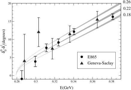
Fig. 3. : Phase relevant for the decay $K\rightarrow\pi\pi e\nu$. The three bands correspond to the three indicated values of the $S$–wave scattering length $a_{0}^{0}$. The uncertainties are dominated by those from the experimental input used in the Roy equations. The triangles are the data points of ref. [29], while the full circles represent the E865 results [10].

The prediction (25) is illustrated in fig. 3, where the energy dependence of the phase difference is shown for $a_{0}^{0}=0.18$, $0.22$ and $0.26$. The width of the corresponding bands indicates the uncertainties, which according to (26) grow in proportion to $q^{3}$ – in the range shown, they amount to less than a third of a degree.

The figure shows that the data of ref. [29] barely distinguish between the three values of $a_{0}^{0}$ shown. The results of the E865 experiment at Brookhaven [10] are significantly more precise, however. The best fit to these data is obtained for $a_{0}^{0}=0.218$, with $\chi^{2}=5.7$ for 5 degrees of freedom. This beautifully confirms the value in eq. (23), obtained on the basis of standard chiral perturbation theory. There is a marginal problem only with the bin of lowest energy: the corresponding scattering lengths are outside the region where the Roy equations admit solutions. In view of the experimental uncertainties attached to that point, this discrepancy is without significance: the difference between the central experimental value and the prediction amounts to 1.5 standard deviations. Note also that the old data are perfectly consistent with the new ones: the overall fit yields $a_{0}^{0}=0.221$ with $\chi^{2}=8.3$ for 10 degrees of freedom.

The relation (25) can be inverted, so that each one of the values found for the phase difference yields a measurement of the scattering length $a_{0}^{0}$. The result is shown in fig. 4. The experimental errors are remarkably small. It is not unproblematic, however, to treat the data collected in the different bins as statistically independent: in the presence of correlations, this procedure underestimates the actual uncertainties. Also, since the phase difference rapidly rises with the energy, the binning procedure may introduce further uncertainties. To account for this, the final result given in ref. [9],

$$a_{0}^{0}=0.221\pm 0.026\;,$$ (27)

corresponds to the 95% confidence limit – in effect, this amounts to stretching the statistical error bar by a factor of two.

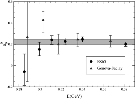
Fig. 4. : $K_{e_{4}}$ data on the scattering length $a_{0}^{0}$. The triangles are the data points of ref. [29], while the full circles represent the E865 results [10]. The horizontal band indicates the statistical average of the 11 values for $a_{0}^{0}$ shown in the figure.

We may translate the result into an estimate for the magnitude of the coupling constant $\bar{\ell}_{3}$: the range (27) corresponds to $|\bar{\ell}_{3}|\,\,\raisebox{-3.00003pt}{$\stackrel{{\scriptstyle\raisebox{-0.70004pt}{$<$}}}{{\sim}}$}\,\,16$. Although this is a coarse estimate, it implies that the Gell-Mann-Oakes-Renner relation does represent a decent approximation: more than 94% of the pion mass stems from the first term in the quark mass expansion (17), i.e. from the term that originates in the quark condensate. This demonstrates that there is no need for a reordering of the chiral perturbation series based on SU(2)${}_{{\scriptscriptstyle R}}\times$SU(2)_L. In that context, the generalized scenario has served its purpose and can now be dismissed.

A beautiful experiment is under way at CERN [30], which exploits the fact that $\pi^{+}\pi^{-}$ atoms decay into a pair of neutral pions, through the strong transition $\pi^{+}\pi^{-}\!\rightarrow\!\pi^{0}\pi^{0}$. Since the momentum transfer nearly vanishes, only the scattering lengths are relevant: at leading order in isospin breaking, the transition amplitude is proportional to $a_{0}^{0}\!-\!a_{0}^{2}$. The corrections at next–to–leading order are now also known [31]. Hence a measurement of the lifetime of a $\pi^{+}\pi^{-}$ atom amounts to a measurement of this combination of scattering lengths. At the planned accuracy of 10% for the lifetime, the experiment will yield a measurement of the scattering lengths to 5%, thereby subjecting chiral perturbation theory to a very sensitive test.

References

- [1] C. Vafa and E. Witten, Nucl. Phys. B 234, 173 (1984).
- [2] W. Heisenberg, Z. Phys. 77, 1 (1932).
- [3] Y. Nambu, Phys. Rev. Lett. 4 (1960) 380; Phys. Rev. 117 (1960) 648.
- [4] M. Gell-Mann, R. J. Oakes and B. Renner, Phys. Rev. 175, 2195 (1968).
- [5] M. Knecht, B. Moussallam, J. Stern and N. H. Fuchs, Nucl. Phys. B 457 (1995) 513 [hep-ph/9507319]; ibid. B 471 (1996) 445 [hep-ph/9512404].
- [6] B. L. Ioffe, Nucl. Phys. B 188 (1981) 317.
- [7] V. Lubicz, Nucl. Phys. B (Proc. Suppl.) 94 (2001) 116 [hep-lat/0012003].
- [8] H. Leutwyler, Phys. Lett. B 378 (1996) 313 [hep-ph/9602366].
- [9] G. Colangelo, J. Gasser and H. Leutwyler, Phys. Rev. Letters 86 (2001) 5008 [hep-ph/0103063].
- [10] S. Pislak et al. [BNL-E865 Collaboration], hep-ex/0106071.
- [11] S. Weinberg, Physica A 96, 327 (1979).
- [12] J. Gasser and H. Leutwyler, Annals Phys. 158, 142 (1984).
-
[13]
For recent reviews of the method, I refer to:
J. Bijnens and U. Meissner, hep-ph/9901381;
G. Colangelo, hep-ph/0001256; hep-ph/0011025;
A. Dobado, A. Gomez-Nicola, J. P. Maroto and J. P. Pelaez, Effective Lagrangians for the Standard Model, Springer, N.Y. 1997;
G. Ecker, hep-ph/9805500; hep-ph/0011026;
J. Gasser, Nucl. Phys. Proc. Suppl. 86, 257 (2000); hep-ph/9906543;
Barry R. Holstein, hep-ph/0001281;
H. Leutwyler, hep-ph/0008124;
U. Meissner, Rep. Prog. Phys. 56, 903 (1993);
A. Pich, hep-ph/9806303;
Jose Wudka, hep-ph/0002180. -
[14]
The foundations of the method are discussed in detail in
H. Leutwyler, Ann. Phys. (N.Y.) 235 (1994) 165. - [15] H. Leutwyler, Nucl. Phys. B (Proc. Suppl.) 94 (2001) 108 [hep-ph/0011049].
- [16] G. Colangelo, Phys. Lett. B 350 85 (1995); ibid. B 361, 234 (1995) (E).
- [17] G. Colangelo, J. Gasser and H. Leutwyler, Nucl. Phys. B 603 (2001) 125 [hep-ph/0103088].
- [18] J. Heitger, R. Sommer and H. Wittig [ALPHA Collaboration], Nucl. Phys. B 588 (2000) 377 [hep-lat/0006026].
- [19] S. Dürr, hep-lat/0103011.
- [20] J. F. Donoghue, J. Gasser and H. Leutwyler, Nucl. Phys. B 343 (1990) 341.
- [21] S. M. Roy, Phys. Lett. B 36 (1971) 353.
-
[22]
B. Ananthanarayan, G. Colangelo, J. Gasser and H. Leutwyler,
Phys. Reports 353 (2001) 207. - [23] S. Weinberg, Phys. Rev. Lett. 17, 616 (1966).
-
[24]
J. Bijnens, G. Colangelo, G. Ecker, J. Gasser and M. E. Sainio,
Phys. Lett. B 374, 210 (1996), Nucl. Phys. B 508, 263 (1997);
ibid. B 517, 639 (1998) (E). - [25] G. Amoros, J. Bijnens and P. Talavera, Nucl. Phys. B 585 (2000) 293, ibid. B 598 (2000) 293 (E) [hep-ph/0003258].
- [26] G. Colangelo, J. Gasser and H. Leutwyler, Phys. Lett. B 488, 261 (2000).
- [27] J. Gasser and H. Leutwyler, Phys. Lett. B 125 (1983) 325.
-
[28]
C. D. Froggatt and J. L. Petersen,
Nucl. Phys. B 129 (1977) 89;
M. M. Nagels et al., Nucl. Phys. B 147 (1979) 189. - [29] L. Rosselet et al., Phys. Rev. D 15 (1977) 574.
-
[30]
B. Adeva et al., CERN proposal CERN/SPSLC 95-1 (1995);
http://dirac.web.cern.ch/DIRAC/. -
[31]
J. Gasser, V. E. Lyubovitskij and A. Rusetsky,
Phys. Lett. B 471 (1999) 244
[hep-ph/9910438];
H. Sazdjian, Phys. Lett. B 490 (2000) 203 [hep-ph/0004226] and references therein.