Electromagnetic form factor of the pion

Abstract

The Standard Model prediction for the magnetic moment of the muon requires a determination of the electromagnetic form factor of the pion at high precision. It is shown that the recent progress in $\pi\pi$ scattering allows us to obtain an accurate representation of this form factor on the basis of the data on $e^{+}e^{-}\rightarrow\pi^{+}\pi^{-}$. The same method also applies to the form factor of the weak vector current, where the data on the decay $\tau\rightarrow\pi^{-}\pi^{0}\,\nu_{\tau}$ are relevant. Unfortunately, however, the known sources of isospin breaking do not explain the difference between the two results. The discrepancy implies that the Standard Model prediction for the magnetic moment of the muon is currently subject to a large uncertainty.

Talk given at the Workshop Continuous Advances in QCD 2002/Arkadyfest
in honor of the 60th birthday of Arkady Vainshtein, Minneapolis, May 2002.

1 Motivation: magnetic moment of the muon

The fabulous precision reached in the measurement of the muon magnetic moment [[1]] allows a thorough test of the Standard Model. The prediction that follows from the Dirac equation, $\mu=e\,\hbar/2m_{\mu}$, only holds to leading order in the expansion in powers of the fine structure constant $\alpha$. It is customary to write the correction in the form

$$\mu=\frac{e\,\hbar}{2\,m_{\mu}}\,(1+a)\;\;.$$ (1)

Schwinger was able to calculate the term of first order in $\alpha$, which stems from the triangle graph in fig. 1a and is universal [[2]],

$$a=\frac{\alpha}{2\pi}+O(\alpha^{2})\;\;.$$ (2)

The contributions of $O(\alpha^{2})$ can also unambiguously be calculated, except for the one from hadronic vacuum polarization, indicated by the graph in fig. 1e. It is analogous to the contributions generated by leptonic vacuum polarization in figs. 1b, 1c and 1d,

	\psfrag{e}{\raisebox{1.00006pt}{$\!e$}}\includegraphics[width=54.06006pt]{graph3.eps}	\psfrag{e}{\raisebox{1.00006pt}{$\!\mu$}}\includegraphics[width=54.06006pt]{graph3.eps}	\psfrag{e}{\raisebox{1.00006pt}{$\!\tau$}}\includegraphics[width=54.06006pt]{graph3.eps}
1a	1b	1c	1d	1e

but involves quarks and gluons instead of leptons. All of these graphs may be viewed as arising from vacuum polarization in the photon propagator:

$$D_{\mu\nu}(q)=\frac{g_{\mu\nu}\,Z}{q^{2}\{1+\Pi(q^{2})\}}+\mbox{gauge terms}\;\;.$$

The expansion of the self energy function $\Pi(t)$ in powers of $\alpha$ starts with

$$\Pi(t)=\alpha\,\Pi^{(0)}(t)+\alpha^{2}\,\Pi^{(1)}(t)+\ldots$$

It is normalized by $\Pi(0)=0$. The leading term can be pictured as

$\Pi^{(0)}(t)=$  \psfrag{e}{\raisebox{1.00006pt}{$\!e$}}\includegraphics[width=19.91684pt]{graph4.eps}  +   \psfrag{e}{\raisebox{1.00006pt}{$\!\mu$}}\includegraphics[width=19.91684pt]{graph4.eps}  +   \psfrag{e}{\raisebox{1.00006pt}{$\!\tau$}}\includegraphics[width=19.91684pt]{graph4.eps} +  

As shown in ref. [[3]], the modification of the Schwinger formula (2) that is generated by vacuum polarization can be represented in compact form:

$$a=\frac{\alpha}{\pi}\int_{0}^{1}\!\!\!dx\,\frac{1-x}{1+\Pi(t_{x})}\;\;,\hskip 20.00003ptt_{x}=-\frac{x^{2}m_{\mu}^{2}}{1-x}\;\;.$$ (3)

Expanding this formula in powers of $\alpha$, we obtain

$$a=\frac{\alpha}{\pi}\int_{0}^{1}\!\!dx\,(1-x)-\frac{\alpha^{2}}{\pi}\int_{0}^{1}\!\!\!dx\,(1-x)\,\Pi^{(0)}(t_{x})+O(\alpha^{3})$$

The first term indeed reproduces the Schwinger formula (2), which corresponds to graph 1a. The term linear in $\Pi^{(0)}(t)$ accounts for graphs 1b to 1e. The contribution involving the square of $\Pi^{(0)}(t)$ describes the one-particle reducible graphs with two bubbles, etc.

The vacuum polarization due to a lepton loop is given by $(\ell=e,\mu,\tau)$

$$\Pi_{\ell}^{(0)}(t) = \frac{t}{3\pi}\int_{4M_{\ell}^{2}}^{\infty}\!\!ds\frac{R_{\ell}(s)}{s(s-t)}\;\;,$$ (4)

$$R_{\ell}(s) = \sqrt{1-\frac{4M_{\ell}^{2}}{s}}\left(1+\frac{2M_{\ell}^{2}}{s}\right)\;\;.$$

The hadronic contribution cannot be calculated analytically, but it can be expressed in terms of the cross section of the reaction $e^{+}e^{-}\rightarrow\mbox{hadrons}$. More precisely, the leading term in the expansion of this cross section in powers of $\alpha$,

$$\sigma_{e^{+}e^{-}\rightarrow h}=\alpha^{2}\sigma_{e^{+}e^{-}\rightarrow h}^{(0)}+O(\alpha^{3})\;\;,$$

is relevant. In terms of this quantity the expression reads

$$\Pi_{h}^{(0)}(t) = \frac{t}{3\pi}\int_{4M_{\pi}^{2}}^{\infty}\!\!ds\frac{R_{h}(s)}{s(s-t)}\;\;,$$ (5)

$$R_{h}(s) = \frac{3s}{4\pi}\,\sigma_{e^{+}e^{-}\rightarrow h}^{(0)}(s)\;\;.$$

At low energies, where the final state necessarily consists of two pions, the cross section is given by the square of the electromagnetic form factor of the pion,

$$R_{h}(s)=\frac{1}{4}\left(1-\frac{4M_{\pi}^{2}}{s}\right)^{\frac{3}{2}}\,|F(s)|^{2}\;\;,\hskip 20.00003pts<9\,M_{\pi}^{2}\;\;.$$ (6)

Numerically, the contribution from hadronic vacuum polarization to the magnetic moment of the muon amounts to $a_{\mbox{\tiny hvp}}\simeq 700\times 10^{-10}$. This is a small fraction of the total, $a=11\,659\,203\,(8)\times 10^{-10}$ [[1]], but large compared to the experimental uncertainty: a determination of $a_{\mbox{\tiny hvp}}$ to about 1% is required for the precision of the Standard Model prediction to match the experimental one. Since the contribution from hadronic vacuum polarization is dominated by the one from the two pion states, this means that the pion form factor is needed to an accuracy of about half a percent.

2 Comparison of leptonic and hadronic contributions

Graphically, the formula (6) amounts to

$\Rightarrow$    \psfrag{pi}{\raisebox{1.00006pt}{$\!\pi$}}\includegraphics[width=56.9055pt]{graph6.eps}

There are three differences between the pionic loop integral and those belonging to the lepton loops:

• the masses are different

• the spins are different

• the pion is composite – the Standard Model leptons are elementary

The compositeness manifests itself in the occurrence of the form factor $F(s)$, which generates an enhancement: at the $\rho$ peak, $|F(s)|^{2}$ reaches values of order 45. The remaining difference in the expressions for the quantities $R_{\ell}(s)$ and $R_{h}(s)$ in eqs. (4) and (6) originates in the fact that the leptons carry spin $\frac{1}{2}$, while the spin of the pion vanishes. Near threshold, the angular momentum barrier suppresses the function $R_{h}(s)$ by three powers of momentum, while $R_{\ell}(s)$ is proportional to the first power. The suppression largely compensates the enhancement by the form factor – by far the most important property is the mass: in units of $10^{-10}$, the contributions due to the $e,\mu$ and $\tau$ loops are 59040.6, 846.4 and 4.2, respectively, to be compared with the 700 units from hadronic vacuum polarization. The latter is comparable to the one from the muon – in accordance with the fact that the masses of pion and muon are similar.

3 Pion form factor

In the following, I disregard the electromagnetic interaction – the discussion concerns the properties of the form factor in QCD. I draw from ongoing work carried out in collaboration with Irinel Caprini, Gilberto Colangelo, Simon Eidelman, Jürg Gasser and Fred Jegerlehner.

The systematic low energy analysis of the form factor based on chiral perturbation theory [[5]] has been worked out to two loops [[6]]. This approach, however, only covers the threshold region. The range of validity of the representation can be extended to higher energies by means of dispersive methods [[7]], which exploit the constraints imposed by analyticity and unitarity. Our approach is very similar to the one of de Trocóniz and Yndurain [[8]]. For a thorough discussion of the mathematical framework, I refer to Heyn and Lang [[9]].

We represent the form factor as a product of three functions that account for the prominent singularities in the low energy region:

$$F(s)=G_{2}(s)\times G_{3}(s)\times G_{4}(s)\;\;.$$ (7)

The index has to do with the number of pions that generate the relevant discontinuity: two in the case of $G_{2}$, three for $G_{3}$ and four or more for $G_{4}$.

The first term represents the familiar Omnès factor that describes the branch cut due to $\pi^{+}\pi^{-}$ intermediate states (states with two neutral pions do not contribute, because the matrix element $\langle\pi^{0}\pi^{0}\,\mbox{out}\,|\,j^{\mu}\,|0\rangle$ vanishes, on account of Bose statistics). The corresponding branch point singularity is of the type $\mbox{Im}\,G_{2}(s)\sim(s-s_{2})^{\frac{3}{2}}$, with $s_{2}=4M_{\pi}^{2}$. The Watson final state interaction theorem implies that, in the elastic region, $4M_{\pi}^{2}<s<9M_{\pi}^{2}$, the phase of the form factor is given by the P-wave phase shift of the elastic scattering process $\pi^{+}\pi^{-}\rightarrow\pi^{+}\pi^{-}$. Denoting this phase shift by $\delta(s)$, the explicit expression for the Omnès factor reads:

$$G_{2}(s)=\exp\left\{\frac{s}{\pi}\int_{4M_{\pi}^{2}}^{\infty}\frac{dx\;\delta(x)}{x\,(x-s)}\right\}\;\;.$$ (8)

The function $G_{3}(s)$ contains the singularities generated by $3\pi$ intermediate states: $G_{3}(s)$ is analytic except for a cut starting at $s_{3}=9M_{\pi}^{2}$, with a branch point singularity of the type $\mbox{Im}\,G_{3}(s)\sim(s-s_{3})^{4}$. If isospin symmetry were exact, the form factor would not contain such singularities: in the limit $m_{u}=m_{d}$, the term $G_{3}(s)$ is equal to 1. Indeed, isospin is nearly conserved, but the occurrence of a narrow resonance with the proper quantum numbers strongly enhances the effects generated by isospin breaking: the form factor contains a pole close to the real axis,

$$G_{3}(s)=1+\epsilon\,\frac{s}{s_{\omega}-s}+\ldots\hskip 20.00003pts_{\omega}=(M_{\omega}-\mbox{$\frac{1}{2}$}\,i\,\Gamma_{\omega})^{2}\;\;.$$ (9)

This implies that, in the vicinity of $s=M_{\omega}^{2}$, the form factor rapidly varies, both in magnitude and in phase. The pole term cannot stand by itself because it fails to be real in the spacelike region. We replace it by a dispersion integral with the proper behaviour at threshold, but this is inessential: in the experimental range, the representation for $G_{3}(s)$ that we are using can barely be distinguished from the pole approximation (9).

Isospin breaking also affects the scattering amplitude. In particular, it gives rise to the inelastic reaction $2\pi\rightarrow 3\pi$, with an amplitude proportional to $m_{u}-m_{d}$. Hence unitarity implies that, in the region $9M_{\pi}^{2}<s<16M_{\pi}^{2}$, the elasticities of the partial waves are less than 1. Numerically, the effect is tiny, however, because it is of second order in $m_{u}-m_{d}$. To a very high degree of accuracy, the first two terms in eq. (7) thus account for all singularities below $s_{4}=16M_{\pi}^{2}$ – the function $G_{4}(s)$ is analytic in the plane cut from $s_{4}$ to $\infty$. Phase space strongly suppresses the strength of the corresponding branch point singularity: $\mbox{Im}\,G_{4}(s)\propto(s-s_{4})^{\frac{9}{2}}$. A significant discontinuity due to inelastic channels only manifests itself for $s>s_{in}=(M_{\omega}+M_{\pi})^{2}$.

We analyze the background term $G_{4}(s)$ by means of a conformal mapping. The transformation

$$z=\frac{\sqrt{s_{in}-s_{1}}\,-\sqrt{s_{in}-s}}{\sqrt{s_{in}-s_{1}}\,+\sqrt{s_{in}-s}}$$ (10)

maps the $s$-plane cut along $s>s_{in}$ onto the unit disk in the $z$-plane, so that the Taylor series expansion in powers of $z$ converges on the entire physical sheet, irrespective of the value of the arbitrary parameter $s_{1}$. We truncate this series after the first few terms, thus approximating the function $G_{4}(s)$ by a low order polynomial in $z$.

4 Roy equations

The crucial element in the above representation is the phase $\delta(s)$. The main difference between our analysis and the one in ref. [[8]] concerns the input used to describe the behaviour of this phase. In fact, during the last two or three years, our understanding of the $\pi\pi$ scattering amplitude has made a quantum jump. As a result of theoretical work [[10]–[12]], the low energy behaviour of the S- and P-waves is now known to an amazing accuracy – to my knowledge, $\pi\pi$ scattering is the only field in strong interaction physics where theory is ahead of experiment.

The method used to implement the requirements of analyticity, unitarity and crossing symmetry is by no means new. As shown by Roy more than 30 years ago [[13]], these properties of the scattering amplitude subject the partial waves to a set of coupled integral equations. These equations involve two subtraction constants, which may be identified with the two $S$–wave scattering lengths $a_{0}^{0}$, $a_{0}^{2}$. If these two constants are given, the Roy equations allow us to calculate the scattering amplitude in terms of the imaginary parts above the ”matching point” $E_{m}=0.8\,\mbox{GeV}$. The available experimental information suffices to evaluate the relevant dispersion integrals, to within small uncertainties [[10, 12]]. In this sense, $a_{0}^{0}$, $a_{0}^{2}$ represent the essential parameters in low energy $\pi\pi$ scattering.

As will be discussed in some detail in the next section, chiral symmetry predicts the values of the two subtraction constants and thereby turns the Roy equations into a framework that fully determines the low energy behaviour of the $\pi\pi$ scattering amplitude. In particular, the P-wave scattering length and effective range are predicted very accurately: $a_{1}^{1}=0.0379(5)\,M_{\pi}^{-2}$ and $b_{1}^{1}=0.00567(13)\,M_{\pi}^{-4}$. The manner in which the P-wave phase shift passes through 90^∘ when the energy reaches the mass of the $\rho$ is specified within the same framework, as well as the behaviour of the two S-waves. The analysis reveals, for instance, that the isoscalar S-wave contains a pole on the second sheet and the position can be calculated rather accurately: the pole occurs at $E=M_{\sigma}-\frac{1}{2}\,i\,\Gamma_{\sigma}$, with $M_{\sigma}=470\pm 30\;\mbox{MeV}$, $\Gamma_{\sigma}=590\pm 40\;\mbox{MeV}$ [[11]], etc.

Many papers based on alternative approaches can be found in the literature. Padé approximants, for instance, continue to enjoy popularity and the ancient idea that the $\sigma$ pole represents the main feature in the isoscalar S-wave also found new adherents recently. Crude models such as these may be of interest in connection with other processes where the physics yet remains to be understood, but for the analysis of the $\pi\pi$ scattering amplitude, they cannot compete with the systematic approach based on analyticity and chiral symmetry. In view of the precision required in the determination of the pion form factor, ad hoc models are of little use, because the theoretical uncertainties associated with these are too large.

5 Prediction for the $\pi\pi$ scattering lengths

Goldstone bosons of zero momentum do not interact: if the quark masses $m_{u},m_{d}$ are turned off, the S-wave scattering lengths disappear, $a_{0}^{0},a_{0}^{2}\rightarrow 0$. Like the mass of the pion, these quantities represent effects that arise from the breaking of the chiral symmetry generated by the quark masses. In fact, as shown by Weinberg [[14]], $a_{0}^{0}$ and $a_{0}^{2}$ are proportional to the square of the pion mass

$$a_{0}^{0}=\frac{7M_{\pi}^{2}}{32\pi F_{\pi}^{2}}+O(M_{\pi}^{4})\;\;,\hskip 20.00003pta_{0}^{2}=-\frac{M_{\pi}^{2}}{16\pi F_{\pi}^{2}}+O(M_{\pi}^{4})\;\;.$$

The corrections of order $M_{\pi}^{4}$ contain chiral logarithms. In the case of $a_{0}^{0}$, the logarithm has an unusually large coefficient

$$a_{0}^{0}=\frac{7M_{\pi}^{2}}{32\pi F_{\pi}^{2}}\left\{1+\frac{9}{2}\,\frac{M_{\pi}^{2}}{(4\pi F_{\pi})^{2}}\,\ln\frac{\Lambda_{0}^{2}}{M_{\pi}^{2}}+O(M_{\pi}^{4})\right\}\;\;.$$

This is related to the fact that in the channel with $I=0$, chiral symmetry predicts a strong, attractive, final state interaction. The scale $\Lambda_{0}$ is determined by the coupling constants of the effective Lagrangian of $O(p^{4})$:

$$\frac{9}{2}\ln\frac{\Lambda_{0}^{2}}{M_{\pi}^{2}}=\frac{20}{21}\,\mbox{\large$\bar{\ell}_{1}$}+\frac{40}{21}\,\mbox{\large$\bar{\ell}_{2}$}-\frac{5}{14}\,\mbox{\large$\bar{\ell}_{3}$}+2\,\mbox{\large$\bar{\ell}_{4}$}+\frac{5}{2}\;\;.$$

The same coupling constants also determine the first order correction in the low energy theorem for $a_{0}^{2}$.

The couplings $\bar{\ell}_{1}$ and $\bar{\ell}_{2}$ control the momentum dependence of the scattering amplitude at first nonleading order. Using the Roy equations, these constants can be determined very accurately [[11]]. The terms $\bar{\ell}_{3}$ and $\bar{\ell}_{4}$, on the other hand, describe the dependence of the scattering amplitude on the quark masses – since these cannot be varied experimentally, $\bar{\ell}_{3}$ and $\bar{\ell}_{4}$ cannot be determined on the basis of $\pi\pi$ phenomenology. The constant $\bar{\ell}_{3}$ specifies the correction in the Gell-Mann-Oakes-Renner relation [[15]],

$$M_{\pi}^{2}=M^{2}\left\{1-\frac{1}{2}\,\frac{M^{2}}{(4\,\pi F)^{2}}\;\bar{\ell}_{3}+O(M^{4})\right\}\;\;.$$ (11)

Here $M^{2}$ stands for the term linear in the quark masses,

$$M^{2}=(m_{u}+m_{d})\,|\langle 0|\,\bar{u}u\,|0\rangle|\,\frac{1}{F^{2}}$$ (12)

($F$ and $\langle 0|\,\bar{u}u\,|0\rangle$ are the values of the pion decay constant and the quark condensate in the chiral limit, respectively). The coupling constant $\bar{\ell}_{4}$ occurs in the analogous expansion for $F_{\pi}$,

$$F_{\pi}=F\left\{1+\frac{M^{2}}{(4\,\pi F)^{2}}\;\bar{\ell}_{4}+O(M^{4})\right\}\;\;.$$ (13)

A low energy theorem relates it to the scalar radius of the pion [[16]],

$$\langle r^{2}\rangle\!\rule[-3.00003pt]{0.0pt}{0.0pt}_{s}=\frac{6}{(4\pi F)^{2}}\left\{\bar{\ell}_{4}-\frac{13}{12}+O(M^{2})\right\}\;\;.$$ (14)

The dispersive analysis of the scalar pion form factor in ref. [[11]] leads to

$$\langle r^{2}\rangle\!\rule[-3.00003pt]{0.0pt}{0.0pt}_{s}=0.61\pm 0.04\;\mbox{fm}^{2}\;\;.$$ (15)

The constants $\bar{\ell}_{1},\ldots\bar{\ell}_{4}$ depend logarithmically on the quark masses:

$$\bar{\ell}_{i}=\ln\frac{\Lambda_{i}^{2}}{M^{2}}\;\;,\hskip 20.00003pti=1,\ldots,4$$

In this notation, the above value of the scalar radius amounts to

$$\Lambda_{4}=1.26\pm 0.14\;\mbox{GeV}\;\;.$$ (16)

Unfortunately, the constant $\bar{\ell}_{3}\leftrightarrow\Lambda_{3}$ is not known with comparable precision. The crude estimate for $\bar{\ell}_{3}$ given in ref. [[16]] corresponds to

$$0.2\;\mbox{GeV}<\Lambda_{3}<2\;\mbox{GeV}\;\;.$$ (17)

\psfrag{a00}{\raisebox{-10.00002pt}{\Large$a_{0}^{0}$}}\psfrag{a20}{\Large$a_{0}^{2}$}\includegraphics[width=256.0748pt,angle={-90}]{a0a2arkady.ps}

Figure 2: Prediction for the S-wave $\pi\pi$ scattering lengths

It turns out, however, that the contributions from $\bar{\ell}_{3}$ are very small, so that the uncertainty in $\Lambda_{3}$ does not strongly affect the predictions for the scattering lengths. This is shown in fig. 2, where the values of $a_{0}^{0}$, $a_{0}^{2}$ predicted by ChPT are indicated as a small ellipse.

6 Experimental test

Stern and collaborators [[17]] pointed out that ”Standard” ChPT relies on a hypothesis that calls for experimental test. Such a test has now been performed and I wish to briefly describe this development.

The hypothesis in question is the assumption that the quark condensate represents the leading order parameter of the spontaneously broken chiral symmetry. More specifically, the standard analysis assumes that the term linear in the quark masses dominates the expansion of $M_{\pi}^{2}$. According to the Gell-Mann-Oakes-Renner relation (12), this term is proportional to the quark condensate, which in QCD represents the order parameter of lowest dimension. The dynamics of the ground state is not well understood. The question raised by Stern et al. is whether, for one reason or the other, the quark condensate might turn out to be small, so that the Gell-Mann-Oakes-Renner formula would fail – the ”correction” might be comparable to or even larger than the algebraically leading term.

According to eq. (11), the correction is determined by the effective coupling constant $\bar{\ell}_{3}$. The estimate (17) implies that the correction amounts to at most 4% of the leading term, but this does not answer the question, because that estimate is based on the standard framework, where $\langle 0|\,\bar{u}u\,|0\rangle$ is assumed to represent the leading order parameter. If that estimate is discarded and $\bar{\ell}_{3}$ is treated as a free parameter (”Generalized” ChPT), the scattering lengths cannot be predicted individually, but the low energy theorem (14) implies that – up to corrections of next-to-next-to leading order – the combination $2a_{0}^{0}-5a_{0}^{2}$ is determined by the scalar radius:

$$2a_{0}^{0}-5a_{0}^{2}=\frac{3M_{\pi}^{2}}{4\,\pi F_{\pi}^{2}}\left\{1+\frac{M_{\pi}^{2}\langle r^{2}\rangle\!\rule[-3.00003pt]{0.0pt}{0.0pt}_{s}}{3}+\frac{41M_{\pi}^{2}}{192\,\pi^{2}F_{\pi}^{2}}+O(M_{\pi}^{4})\right\}\;\;.$$

The resulting correlation between $a_{0}^{0}$ and $a_{0}^{2}$ is shown as a narrow strip in fig. 2 (the strip is slightly curved because the figure accounts for the corrections of next-to-next-to leading order).

In view of the correlation between $a_{0}^{0}$ and $a_{0}^{2}$, the data taken by the E865-collaboration at Brookhaven [[18]] allow a significant test of the Gell-Mann-Oakes-Renner relation. The final state interaction theorem implies that the phase of the form factors relevant for the decay $K^{+}\rightarrow\pi^{+}\pi^{-}e^{+}\bar{\nu}_{e}$ is determined by the elastic $\pi\pi$ scattering amplitude. Conversely, the phase difference $\delta_{0}^{0}-\delta_{1}^{1}$ can be measured in this decay. The analysis of the $4\cdot 10^{5}$ events of this type collected by E865 leads to the round data points in fig. 3, taken from ref. [[19]] (the triangles represent the $K_{e_{4}}$ data collected in the seventies).

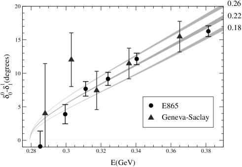
Figure 3: Interpretation of the data on the phase difference $\delta^{1}_{1}-\delta^{0}_{0}$ in Generalized Chiral Perturbation Theory.

The three bands show the result obtained in Generalized ChPT for $a_{0}^{0}=0.18,0.22,0.26$, respectively. The width of the bands corresponds to the uncertainty in the prediction. A fit of the data that exploits the correlation between $a_{0}^{0}$ and $a_{0}^{2}$ yields

$$a_{0}^{0}=0.216\pm 0.013\,(\mbox{stat})\pm 0.004\,(\mbox{syst})\pm 0.005\,(\mbox{th})\;\mbox{[\raisebox{-5.26376pt}[0.0pt][0.0pt]{\Large\cite[cite]{[\@@bibref{}{Brookhaven}{}{}]}}]}\;\;,$$

where the third error bar accounts for the theoretical uncertainties. The result thus beautifully confirms the prediction of ChPT, $a_{0}^{0}=0.220\pm 0.005$. The agreement implies that more than 94% of the pion mass originate in the quark condensate, thus confirming that the Gell-Mann-Oakes-Renner relation is approximately valid [[19]]. May Generalized ChPT rest in peace.

7 Comparison of electromagnetic and weak form factors

In the theoretical limit $m_{u}=m_{d}$ and in the absence of the electromagnetic interaction, the vector current relevant for strangeness conserving semileptonic transitions is conserved. The matrix element of this current that shows up in the decay $\tau\rightarrow\pi^{-}\pi^{0}\,\nu_{\tau}$ is then determined by the electromagnetic form factor of the pion. In reality, however, $m_{u}$ differs from $m_{d}$ and the radiative corrections in $\tau$ decay are different from those relevant for $e^{+}e^{-}\rightarrow\pi^{+}\pi^{-}$. For the anomalous moment of the muon, $\tau$ decays are of interest only to the extent that these isospin breaking effects are understood, so that the e.m. form factor can be calculated from the weak transition matrix element.

The leading isospin breaking effects are indeed well understood: those enhanced by the small energy denominator associated with $\omega$ exchange, which are described by the factor $G_{3}(s)$ introduced in section 3. As these do not show up in the weak transition matrix element, they must be corrected for when calculating the electromagnetic form factor from $\tau$ decays.

There is another effect that shows up in the process $e^{+}e^{-}\rightarrow\pi^{+}\pi^{-}$, but does not affect $\tau$ decay: vacuum polarization in the photon propagator, as illustrated by the graphs below:

$+$$+$

The same graphs also show up in the magnetic moment of the muon:

    $+$      $+$    $+\;\ldots$

To avoid double counting, the data on the reaction $e^{+}e^{-}\rightarrow\pi^{+}\pi^{-}$ must be corrected for vacuum polarization, multiplying the cross section by the factor $|1+\Pi(s)|^{2}$. In the timelike region, this factor is less than 1, so that the correction reduces the magnitude of the form factor. In the $\omega$ region, the vacuum polarization due to $3\pi$ intermediate states generates a pronounced structure in $\Pi(s)$. While below that energy, the correction is of order 1%, it reaches about 7% immediately above the $\omega$ and then decreases to about 3% towards the upper end of the range covered by the CMD2 data [[20]].

Unfortunately, applying the two corrections just discussed, the results for the form factor obtained with $e^{+}e^{-}$ collisions are systematically lower than those found in $\tau$ decays [[21]–[23]]. The two phenomena mentioned above are not the only isospin breaking effects. Radiative corrections must be applied, to $e^{+}e^{-}$ collisions [[24]] as well as to $\tau$ decays [[25]] and terms of order $m_{u}-m_{d}$ need to be estimated as well. I do not know of a mechanism, however, that could give rise to an additional isospin breaking effect of the required order of magnitude.

One way to quantify the discrepancy is to assume that the uncertainties in the overall normalization of some of the data are underestimated. Indeed, if the normalization of either the rate of the decay $\tau\rightarrow\pi^{-}\pi^{0}\,\nu_{\tau}$ or the cross section of the reaction $e^{+}e^{-}\rightarrow\pi^{+}\pi^{-}$ are treated as free parameters, the problem disappears. The renormalization, however, either lowers the ALEPH and CLEO data by about 4% or lifts the CMD2 data by this amount.

While completing this manuscript, a comparison of the $\tau$ and $e^{+}e^{-}$ data appeared [[26]], where the problem is discussed in detail. One way to put the discrepancy in evidence is to compare the observed rate of the decay $\tau\rightarrow\pi^{-}\pi^{0}\nu_{\tau}$ with the prediction that follows from the data on the reaction $e^{+}e^{-}\rightarrow\pi^{+}\pi^{-}$ if the known sources of isospin breaking are accounted for. Using the observed lifetime of the $\tau$, the prediction for the branching ratio of the channel $\tau\rightarrow\pi^{-}\pi^{0}\,\nu_{\tau}$ reads $B_{\mbox{\tiny pred}}=0.2408\pm 0.0031$. The observed value, $B_{\mbox{\tiny obs}}=0.2546\pm 0.0012$, differs from this number at the $4\,\sigma$ level [[26]].

A difference between the $\tau$ and $e^{+}e^{-}$ results existed before, but with the new CMD2 data, where the hadronic part of vacuum polarization is now corrected for, the disagreement has become very serious. The problem also manifests itself in the values for the $\rho$ width quoted by the Particle Data Group [[27]]: the value obtained by CMD2 is substantially lower than the results found by the ALEPH and CLEO collaborations.

So, unless the Standard Model fails here, either the experimental results for the electromagnetic form factor or those for the weak form factor must be incorrect. The preliminary data from KLOE appear to confirm the CMD2 results, but the uncertainties to be attached to that determination of the electromagnetic form factor yet remain to be analyzed.

Currently, the discrepancy between the $e^{+}e^{-}$ and $\tau$ data prevents a test of the Standard Model prediction for the magnetic moment of the muon at an accuracy that would be comparable to the experimental value. The result for the contribution to the muon anomaly due to hadronic vacuum polarization depends on whether the $e^{+}e^{-}$ data or the $\tau$ data are used to evaluate the electromagnetic form factor – according to ref. [[26]], the corresponding central values differ by $17.2\times 10^{-10}$. Compared to this, the estimate $(8\pm 4)\times 10^{-10}$ for the contribution from hadronic light-by-light scattering [[28]–[31]] is a rather precise number.

8 Asymptotic behaviour

The behaviour of the form factor for large spacelike momenta can be predicted on the basis of perturbative QCD [[32]]:

$$F(-Q^{2}) = \frac{64\pi^{2}F_{\pi}^{2}}{\beta_{0}\,Q^{2}L_{Q}}\,\left\{1+B_{2}\,L_{Q}^{-\mbox{\tiny$\frac{50}{81}$}}+B_{4}\,L_{Q}^{-\mbox{\tiny$\frac{364}{405}$}}+O(L_{Q}^{-1})\right\}^{2}\;\;,$$ (18)

$$L_{Q} = \ln\frac{Q^{2}}{\Lambda^{2}}\;\;,\hskip 20.00003pt\beta_{0}=11-\frac{2}{3}N_{f}\;\;.$$

The leading asymptotic term only involves the pion decay constant. The coefficients $B_{2},B_{4}\ldots$ of the fractional logarithmic corrections are related to the pion distribution amplitude or null plane wave function $\psi(x,\mu)$, which is a function of the momentum fraction $x$ of the quark and depends on the scale $\mu$. Normalizing the wave function to the pion decay constant, the expansion in terms of Gegenbauer polynomials starts with

$$\psi(x,\mu) = 6\,x\,(1-x)\left\{1+B_{2}\,L_{\mu}^{-\mbox{\tiny$\frac{50}{81}$}}\,C_{2}^{\frac{3}{2}}(2x\!-\!1)+B_{4}\,L_{\mu}^{-\mbox{\tiny$\frac{364}{405}$}}\,C_{4}^{\frac{3}{2}}(2x\!-\!1)+\ldots\right\}$$

$$C_{2}^{\frac{3}{2}}(z) = \mbox{$\frac{3}{2}$}\,(5z^{2}-1)\;\;,\hskip 10.00002ptC_{4}^{\frac{3}{2}}(z)=\mbox{$\frac{15}{8}$}\,(21z^{4}-14z^{2}+1)\;\;,\hskip 10.00002pt\ldots$$

The wave function cannot be calculated within perturbative QCD and the phenomenological information about the size of the coefficients $B_{2},B_{4},\ldots$ is meagre. It is therefore of interest to see whether the data on the form factor allow us to estimate these terms.

In the representation (7), the asymptotic behaviour of the form factor can be accounted for as follows. One first continues the asymptotic formula (18) into the timelike region and reads off the asymptotic behaviour of the phase of the form factor:

$$\phi(s)\rightarrow\pi+\frac{\pi}{\ln\frac{s}{\Lambda^{2}}}+\ldots$$

If the asymptotic behaviour of the phase used for the Omnès factor agrees with this, then the Omnès formula (8) ensures that the ratio $F(s)/G_{2}(s)$ approaches a constant for large spacelike momenta. The value of the constant is determined by $F_{\pi}$ and by the behaviour of the phase shift at nonasymptotic energies. This implies that the background term $G_{4}(s)$ tends to a known constant for large values of $s$, or equivalently, for $z\rightarrow-1$.

The corrections involving fractional logarithmic powers can also be accounted for with a suitable contribution to the phase. For the asymptotic expansion not to contain a term of order $s^{-1/2}$, the derivative of $G_{4}(s)$ with respect to $z$ must vanish at $z=-1$. This then yields a representation of the form factor for which the asymptotic behaviour agrees with perturbative QCD, for any value of the coeffcients $B_{2}$ and $B_{4}$.

We have analyzed the experimental information with a representation of this type, including data in the spacelike region, as well as those available at large timelike momenta [[33]-[37]]. The numerical analysis yet needs to be completed and compared with the results in the literature (for a recent review and references, see for instance [[38]]). Our preliminary results are: If the fractional logarithmic powers are dropped ($B_{2}=B_{4}=0$), we find that the asymptotic formula is reached only at academically high energies. With the value for $B_{2}$ proposed by Chernyak and Zhitnitsky, the situation improves. For the asymptotic behaviour to set in early, an even larger value of $B_{2}$ appears to be required.

This indicates that the leading asymptotic term can dominate the behaviour only for very high energies. A direct comparison of that term with the existing data, which only cover small values of $s$ does therefore not appear to be meaningful.

9 Zeros and sum rules

Analyticity subjects the form factor to strong constraints. Concerning the asymptotic behaviour, I assume that $|\ln F(s)|$ at most grows logarithmically for $|s|\rightarrow\infty$, in any direction of the complex $s$-plane. This amounts to the requirement that a) for a sufficiently large value of $n$, the quantity $|F(s)/s^{n}|$ remains bounded and b) the phase of $F(s)$ at most grows logarithmically, so that the real and imaginary parts of $F(s)$ do not oscillate too rapidly at high energies. In view of asymptotic freedom, I take these properties for granted. If the form factor does not have zeros, the function

$$\psi(s)=\frac{1}{(s_{2}-s)^{\frac{3}{2}}}\ln\frac{F(s)}{F(s_{2})}$$

is then analytic in the cut plane and tends to zero for $|s|\rightarrow\infty$. The branch point singularity at threshold is of the type $\psi(s)\sim(s-s_{2})^{-\frac{1}{2}}$. Hence $\psi(s)$ obeys the unsubtracted dispersion relation

$$\psi(s)=\frac{s}{\pi}\int_{s_{2}}^{\infty}\!dx\,\frac{\mbox{Im}\,\psi(x)}{x\,(x-s)}$$

in the entire cut plane. The discontinuity across the cut is determined by the magnitude of the form factor:

$$\mbox{Im}\,\psi(s)=-\frac{1}{(s-s_{2})^{\frac{3}{2}}}\,\ln\,\rule[-8.00003pt]{0.39993pt}{22.0pt}\,\frac{F(s)}{F(s_{2})}\,\rule[-8.00003pt]{0.39993pt}{22.0pt}\hskip 20.00003pts>s_{2}\;\;.$$

Hence the above dispersion relation amounts to a representation of the form factor in terms of its magnitude in the timelike region:

$$F(s)=\rule[-1.99997pt]{0.39993pt}{10.00002pt}\,F(s_{2})\,\rule[-1.99997pt]{0.39993pt}{10.00002pt}\,\exp\left\{-\frac{(s_{2}-s)^{\frac{3}{2}}}{\pi}\int_{s_{2}}^{\infty}\!\!\frac{dx}{(x-s_{2})^{\frac{3}{2}}(x-s)}\,\ln\,\rule[-8.00003pt]{0.39993pt}{22.0pt}\,\frac{F(x)}{F(s_{2})}\,\rule[-8.00003pt]{0.39993pt}{22.0pt}\,\right\}.$$ (19)

The relation implies, for instance, that the magnitude of the form factor in the timelike region also determines the charge radius.

Since the value at the origin is the charge, $F(0)=1$, the magnitude of the form factor must obey the sum rule

$$\frac{8M_{\pi}^{3}}{\pi}\int_{s_{2}}^{\infty}\frac{ds}{s(s-s_{2})^{\frac{3}{2}}}\;\ln\,\rule[-8.00003pt]{0.39993pt}{22.0pt}\,\frac{F(s)}{F(s_{2})}\,\rule[-8.00003pt]{0.39993pt}{22.0pt}=\ln\,|F(s_{2})|\;\;.$$ (20)

A second sum rule follows from the asymptotic properties. For the quantity $\ln F(s)$ not to grow more rapidly than the logarithm of $s$, the function $\psi(s)$ must tend to zero more rapidly than $1/s$. Hence the magnitude of the form factor must obey the condition

$$\frac{2M_{\pi}}{\pi}\int_{s_{2}}^{\infty}\frac{ds}{(s-s_{2})^{\frac{3}{2}}}\,\ln\,\rule[-8.00003pt]{0.39993pt}{22.0pt}\,\frac{F(s)}{F(s_{2})}\,\rule[-8.00003pt]{0.39993pt}{22.0pt}=0\;\;.$$ (21)

The relations (20) and (21) are necessary and sufficient for the existence of an analytic continuation of the boundary values of $|F(s)|$ on the cut that (a) is free of zeros, (b) satisfies the condition $F(0)=1$ and (c) behaves properly for large values of $|s|$.

The above relations only hold if the form factor does not have zeros. In the scattering amplitude, zeros necessarily occur, as a consequence of chiral symmetry – indeed, the main low energy properties of the scattering amplitude may be viewed as consequences of the Adler zeros [[40]]. For the form factor, however, chiral perturbation theory implies that zeros can only occur outside the range where the low energy expansion holds: For the form factor to vanish, the higher order contributions must cancel the leading term of the chiral perturbation series.

In quantum mechanics, the form factor represents the Fourier transform of the charge density. For the ground state of the hydrogen atom, for instance, the charge density of the electron cloud is proportional to the square of the wave function, which does decrease with distance, so that the corresponding form factor is positive in the spacelike region. It does not have any complex zeros, either. The wave functions of radially excited states, on the other hand, contain nodes, so that the form factor does exhibit zeros. Qualitatively, I expect the properties of the pion charge distribution to be similar to the one of the electron in the ground state of the hydrogen atom – in the null plane picture, the form factor again represents the Fourier transform of the square of the wave function [[41]]. In simple models such as those described in [[42]], the form factor is free of zeros.

The hypothesis that the form factor does not contain zeros can be tested experimentally: The sum rules (20) and (21) can be evaluated with the data on the magnitude of the form factor. The evaluation confirms that the sum rules do hold within the experimental errors, but in the case of the slowly convergent sum rule (21), these are rather large. Alternatively, we may examine the properties of the form factor obtained by fitting the data with the representation (7). By construction, the first two factors in that representation are free from zeros, but the term $G_{4}(s)$ may or may not have zeros. In fact, as we are representing this term by a polynomial in the conformal variable $z$, it necessarily contains zeros in the $z$-plane – their number is determined by the degree of the polynomial. The question is whether some of these occur on the physical sheet of the form factor, that is on the unit disk $|z|\leq 1$. The answer is negative: we invariably find that all of the zeros are located outside the disk. It is clear that zeros at large values of $|s|$ cannot be ruled out on the basis of experiment. In view of asymptotic freedom, however, I think that such zeros are excluded as well.

10 Conclusion

The recent progress in our understanding of $\pi\pi$ scattering provides a solid basis for the low energy analysis of the pion form factor. The main problem encountered in this framework is an experimental one: the data on the processes $e^{+}e^{-}\rightarrow\pi^{+}\pi^{-}$ and $\tau\rightarrow\pi^{-}\pi^{0}\,\nu_{\tau}$ are not consistent with our understanding of isospin breaking. If the data are correct, then this represents a very significant failure of the Standard Model – or at least of our understanding thereof. The discrepancy must be clarified also in order for the accuracy of the Standard Model prediction to become comparable with the fabulous precision at which the magnetic moment of the muon has been measured.

References

- [1] G. W. Bennett et al. [Muon g-2 Collaboration], hep-ex/0208001.
- [2] J. Schwinger, Phys. Rev. 73 (1948) 416.
-
[3]
J. Calmet, S. Narison, M. Perrottet and E. de Rafael,
Phys. Lett. B 61 (1976) 283. - [4] B. Lautrup, Phys. Lett. B 69 (1977) 109.
- [5] J. Gasser and H. Leutwyler, Nucl. Phys. B 250 (1985) 517.
-
[6]
G. Colangelo, M. Finkemeier and R. Urech,
Phys. Rev. D 54 (1996) 4403;
J. Bijnens, G. Colangelo and P. Talavera, JHEP 9805 (1998) 014;
P. Post and K. Schilcher, hep-ph/0112352;
J. Bijnens and P. Talavera, JHEP 0203 (2002) 046. -
[7]
J. F. Donoghue, J. Gasser and H. Leutwyler,
Nucl. Phys. B 343 (1990) 341;
J. Gasser and U. Meißner, Nucl. Phys. B 357 (1991) 90;
J. F. Donoghue and E. S. Na, Phys. Rev. D 56 (1997) 7073;
I. Caprini, Eur. Phys. J. C 13 (2000) 471;
A. Pich and J. Portolés, Phys. Rev. D 63 (2001) 093005;
J. A. Oller, E. Oset and J. E. Palomar, Phys. Rev. D 63 (2001) 114009. - [8] J. F. De Trocóniz and F. J. Yndurain, Phys. Rev. D 65 (2002) 093001.
- [9] M.F. Heyn and C.B. Lang, Z. Phys. C 7 (1981) 169.
-
[10]
B. Ananthanarayan, G. Colangelo, J. Gasser and H. Leutwyler,
Phys. Rept. 353 (2001) 207. - [11] G. Colangelo, J. Gasser and H. Leutwyler, Nucl. Phys. B 603 (2001) 125.
-
[12]
S. Descotes, N. H. Fuchs, L. Girlanda and J. Stern,
Eur. Phys. J. C 24 (2002) 469. - [13] S. M. Roy, Phys. Lett. B 36 (1971) 353.
- [14] S. Weinberg, Phys. Rev. Lett. 17 (1966) 616.
- [15] M. Gell-Mann, R. J. Oakes and B. Renner, Phys. Rev. 175 (1968) 2195.
-
[16]
J. Gasser and H. Leutwyler,
Phys. Lett. B 125 (1983) 325;
Annals Phys. 158 (1984) 142. -
[17]
M. Knecht, B. Moussallam, J. Stern and N. H. Fuchs,
Nucl. Phys. B 457 (1995) 513. ibid. B 471 (1996) 445. - [18] S. Pislak et al. [BNL-E865 Collaboration], Phys. Rev. Lett. 87 (2001) 221801.
- [19] G. Colangelo, J. Gasser and H. Leutwyler, Phys. Rev. Lett. 86 (2001) 5008.
-
[20]
R. R. Akhmetshin et al. [CMD-2 Collaboration],
Phys. Lett. B 527 (2002) 161. - [21] R. Barate et al. [ALEPH Collaboration], Z. Phys. C 76 (1997) 15.
- [22] K. W. Edwards et al. [CLEO Collaboration], Phys. Rev. D 61 (2000) 072003.
- [23] K. Ackerstaff et al. [OPAL Collaboration], Eur. Phys. J. C 7 (1999) 571.
- [24] A. Hoefer, J. Gluza and F. Jegerlehner, Eur. Phys. J. C 24 (2002) 51.
-
[25]
V. Cirigliano, G. Ecker and H. Neufeld,
Phys. Lett. B 513 (2001) 361;
JHEP 0208 (2002) 002. - [26] M. Davier, S. Eidelman, A. Höcker and Z. Zhang, hep-ph/0208177.
- [27] K. Hagiwara et al. [Particle Data Group], Phys. Rev. D 66 (2002) 010001.
- [28] M. Knecht and A. Nyffeler, Phys. Rev. D 65 (2002) 073034.
-
[29]
M. Knecht, A. Nyffeler, M. Perrottet and E. de Rafael,
Phys. Rev. Lett. 88 (2002) 071802. - [30] M. Ramsey-Musolf and M. B. Wise, Phys. Rev. Lett. 89 (2002) 041601.
- [31] E. de Rafael, hep-ph/0208251.
-
[32]
G. P. Lepage and S. J. Brodsky,
Phys. Lett. B 87 (1979) 359;
Phys. Rev. D 22 (1980) 2157;
A. V. Efremov and A. V. Radyushkin, Phys. Lett. B 94 (1980) 245;
Theor. Math. Phys. 42 (1980) 97;
V. L. Chernyak and A. R. Zhitnitsky, JETP Lett. 25 (1977) 510;
Sov. J. Nucl. Phys. 31 (1980) 544;
G. R. Farrar and D. R. Jackson, Phys. Rev. Lett. 43 (1979) 246. - [33] J. Volmer et al. [The Jefferson Lab F(pi) Collaboration], Phys. Rev. Lett. 86 (2001) 1713.
- [34] S. R. Amendolia et al., Nucl. Phys. B 277 (1986) 168.
- [35] C. J. Bebek et al., Phys. Rev. D 17 (1978) 1693.
- [36] D. Bollini et al., Nuovo Cim. Lett. 14 (1975) 4188.
- [37] J. Milana, S. Nussinov and M. G. Olsson, Phys. Rev. Lett. 71 (1993) 2533.
- [38] J. Bijnens and A. Khodjamirian, hep-ph/0206252.
- [39] B. V. Geshkenbein, Yad. Fis. 9 (1969) 1932; Yad. Fis. 13 (1971) 1087; Z. Phys. C 45 (1989) 351; Phys. Rev. D 61 (2000) 033009.
- [40] M.R. Pennington and J. Portolés, Phys. Lett. B 344 (1995) 399.
- [41] H. Leutwyler, Nucl. Phys. B 76 (1974) 413.
- [42] W. Jaus, Phys. Rev. D 44 (1991) 2851.