Nonequilibrium evolution of $\Phi^{4}$ theory in $1+1$ dimensions in the $2PPI$ formalism

Abstract

We consider the out-of-equilibrium evolution of a classical condensate field and its quantum fluctuations for a $\Phi^{4}$ model in $1+1$ dimensions with a symmetric and a double well potential. We use the 2PPI formalism and go beyond the Hartree approximation by including the sunset term. In addition to the mean field $\phi(t)=\left<\Phi\right>$ the 2PPI formalism uses as variational parameter a time dependent mass ${\cal M}^{2}(t)$ which contains all local insertions into the Green function. We compare our results to those obtained in the Hartree approximation. In the symmetric $\Phi^{4}$ theory we observe that the mean field shows a stronger dissipation than the one found in the Hartree approximation. The dissipation is roughly exponential in an intermediate time region. In the theory with spontaneous symmetry breaking, i.e., with a double well potential, the field amplitude tends to zero, i.e., to the symmetric configuration. This is expected on general grounds: in $1+1$ dimensional quantum field theory there is no spontaneous symmetry breaking for $T>0$, and so there should be none at finite energy density (microcanonical ensemble), either. Within the time range of our simulations the momentum spectra do not thermalize and display parametric resonance bands.

I Introduction

There has recently been considerable activity in investigating the nonequilibrium evolution of quantum field theory beyond the large-$N$ approximation. In particular there has been formulated Berges:2001fi ; Aarts:2002dj a systematic approach (2PI-NLO) in which all next-to leading order contributions in the $1/N$ expansion are included, using the CJT or 2PI formalism Cornwall:1974vz generalized to nonequilibrium evolution in Ref. Calzetta:1987ey , using the closed time path (CTP) or Schwinger-Keldysh skform formalism. A similar approximation including some but not all contributions of next-to-next-to leading order is the bare vertex approximation (BVA) Mihaila:2001sr . Numerical simulations have been performed mostly in $1+1$ dimensions, for the classical or quantum $\Phi^{4}$ theory with a symmetric Berges:2001fi ; Aarts:2001yn ; Blagoev:2001ze ; Cooper:2002ze ; Berges:2000ur and with a double well Cooper:2002qd potential. A first simulation in an O$(N)$ model for $N\neq 1$ in $3+1$ dimensions has just appeared Berges:2002cz , for a symmetric potential. The analysis of models with $N\neq 1$ and with spontaneous symmetry breaking, i.e., a Mexican hat potential, should be very important for understanding the rôle of the Goldstone modes and their influence on the phase structure of the theory in a certain approximation.

A more modest step beyond leading order large $N$ has been taken in Ref. Baacke:2001zt , where the Hartree approximation was used in an O$(N)$ model in $3+1$ dimensions. This approach includes some terms of the nonleading orders, but not all of them. Our investigation made evident the role of parametric resonance in the system of “sigma” and “pion” modes, and the role of the Goldstone modes in stabilizing the evolution in the regions where the equilibrium effective potential is complex, features still to be investigated in the systematic $1/N$ motivated approximations.

An approach for including nonleading orders in a self-consistent resummation scheme has been proposed some time ago by Verschelde and collaborators Verschelde:bs ; Coppens:zc , the so-called 2PPI expansion. Like in the 2PI or CJT formalism the mean field and the internal Green functions are determined self-consistently. As in the 2PI formalism the equations of motion follow from an effective action, which here is a functional of a mean field $\phi=\left<\Phi\right>$ and an effective mass ${\cal M}$. In contrast to the 2PI approach only local insertions into the Green function are resummed, so the Green function is, in all orders, a functional of the local mass term ${\cal M}$ that in general will depend on $x=(t,{\bf x})$. In particular this Green function is different from the physical Green function. As far as the resummation is concerned the approach is less powerful: one has to include more diagrams if one wants to reach the same order in a loop or $1/N$ expansion as in the 2PI expansion. The fact that the propagators have a simpler structure may be a disadvantage as by this structure the approximation is less flexible than 2PI. On the other hand the calculations are technically less involved, in particular the formalism does not require ladder resummations which complicate the renormalization of the 2PI approach vanHees:2001ik . In one-loop order the approach is equivalent to the Hartree approximation. Recent progress in the 2PPI formalism includes the demonstration or renormalizability Verschelde:2000ta ; Verschelde:2000dz and some finite-temperature two-loop calculations in $3+1$ dimensions. An interesting result was that for $N=1$ Smet:2001un and for $N\neq 1$ Baacke:2002pi the order of the phase transition between the spontaneously broken and symmetric phases becomes second order in the 2-loop approximation, while it is first order in the Hartree approximation. The results for the 2PPI expansion have been compared to exact results in Okopinska:1995mi for the anharmonic oszillator; even more recently Dudal:2002zn the two-loop approximation has been compared, in $1+1$ dimensions, with exact results of the Gross-Neveu model.

In this paper we will present the formulation and some numerical results for the nonequilibrium evolution of the mean field and the self-consistent mass in the 2PPI scheme, applied to $\Phi^{4}$ theory in $1+1$ dimensions. We go beyond the one-loop (Hartree) approximation by including the sunset graph, which represents the full two-loop contribution in this formalism. We explicitly formulate a conserved energy functional which is used to monitor the numerical accuracy. As this is the first investigation of the 2PPI formalism at two loops out of equilibrium we do not attempt a detailed study; rather we aim at presenting the main new features of this approach, as well as compared to the one-loop Hartree approximation and as compared to the other approaches (2PI-NLO and BVA) mentioned above. We consider both the case of the symmetric $\Phi^{4}$ potential and the case of the double well potential which displays spontaneous symmetry breaking on the classical as well as on the one-loop level.

The plan of the paper is as follows: In section 2 we formulate the model and present the 2PPI formalism as applied to the system out of equilibrium. In section 3 we specify the two-loop approximation by giving the explicit expressions for the basic graphs, the equations of motion, the conserved energy and by discussing the initial conditions and renormalization. In section 4 we give details of the numerical implementation. The numerical results are presented and discussed in section 5. We end with conclusions and an outlook in section 6. The paper is completed by two appendices.

II Formulation of the model

We consider the $\Phi^{4}$ quantum field theory defined by the Lagrange density

$${\cal L}=\frac{1}{2}\partial_{\mu}{\Phi}\,\partial^{\mu}{\Phi}-\frac{1}{2}m^{2}\Phi^{2}-\frac{\lambda}{24}\Phi^{4}\;.$$ (2.1)

If $m^{2}>0$ we refer to as the symmetric theory, and with $m^{2}<0$ which we refer to as theory with spontaneous symmetry breaking. These terms relate to the classical theory and do not imply the occurrence of spontaneous symmetry breaking in the quantum field theory.

The 2PPI formalism proposed by Verschelde and Coppens Verschelde:bs ; Coppens:zc is based on an effective action which is formulated in terms of a mean field $\phi$ and a local insertion $\Delta$. It is the Legendre transformation of a generating functional with a source $J(x)$ for the field $\phi(x)$ and another local source $K(x)$ for $\phi^{2}(x)$. Here lies the difference to the well-known CJT formalism, where one introduces a bilocal source $K(x,x^{\prime})$ for a Green function $G(x,x^{\prime})$. Graphically the 2PPI scheme resums all local insertion into a Green function which in all orders remains a generalized free particle Green function, or Green function in an external field, i.e.

$$G^{-1}(x,x^{\prime})=i\left[\Box+{\cal M}^{2}(x)\right]\delta(x-x^{\prime})\ ,$$ (2.2)

where

$${\cal M}^{2}(x)=m^{2}+\frac{\lambda}{2}\phi^{2}(x)+\frac{\lambda}{2}\Delta(x)\;.$$ (2.3)

So in contrast to the 2PI formalism this Green function is not a variational object, it is a functional of ${\cal M}^{2}(x)$. It is not the physical Green function.

The 2PPI formalism in its original form is based on the action

$$\Gamma[\phi,\Delta]=S_{\rm class}[\phi]+\Gamma^{\rm 2PPI}[\phi,{\cal M}^{2}]+\frac{\lambda}{8}\int d^{2}x\Delta^{2}(x)\;.$$ (2.4)

Here $\Gamma^{\rm 2PPI}[\phi,{\cal M}^{2}]$ is the sum of all 2PPI graphs; these are defined as graphs which do not decay into two parts of two lines joining at a point are cut. In the 2PI formalism one includes into the analogous $\Gamma^{\rm 2PI}$ all graphs which do not decay into two parts if any two lines are cut. In order to visualize the difference we show examples of 2PR and 2PPR graphs in Fig. 1. It should be emphasized that in the 2PPI formalism the lines in the graphs are Green functions with the variational mass term ${\cal M}^{2}(x)$ as defined via Eq. (2.2), while in the 2PI formalism the internal lines refer to the variational Green functions induced by the bilocal sources. When comparing the sets of irreducible graphs in both formalisms one has to take into account this difference in the meaning of internal lines.

(a)          (b) 

Figure 1: Examples for two particle point reducible (2PPR) and irreducible (2PPI) diagrams: (a) a diagram which is 2PR and 2PPR (b) a diagram which is 2PR but 2PPI; solid lines: internal propagators; dashed lines: external fields $\phi$.

The insertion $\Delta(x)$ is given by

$$\Delta(x)=-2\frac{\delta\Gamma^{\rm 2PPI}[\phi,{\cal M}^{2}]}{\delta{\cal M}^{2}(x)}\ .$$ (2.5)

As we have stated before it is simpler to formulate the action in terms of $\phi$ and ${\cal M}^{2}$. We solve Eq. (2.3) with respect to $\Delta$ and insert this into Eq. (2.4). Using the explicit form of $S_{\rm class}$ we obtain

$$\Gamma[\phi,{\cal M}^{2}] = \int d^{2}x\left[\frac{1}{2}\partial_{\mu}\phi(x)\,\partial^{\mu}\phi(x)-\frac{1}{2}{\cal M}^{2}(x)\phi^{2}(x)\right.$$ (2.6)

$$\hskip 28.45274pt+\left.\frac{\lambda}{12}\phi^{4}(x)\right]$$

$$+\frac{1}{2\lambda}\int d^{2}x\left[{\cal M}^{2}(x)-m^{2}\right]^{2}$$

$$+\Gamma^{\rm 2PPI}[\phi,{\cal M}^{2}]\;.$$

One easily checks that the equations of motion obtained by varying this action with respect to $\phi(x)$ and ${\cal M}^{2}(x)$ take the form

$$0 = \Box\phi+{\cal M}^{2}(x)\phi(x)-\frac{\lambda}{3}\phi^{3}(x)$$ (2.7)

$$\hskip 56.9055pt-\frac{\delta\Gamma^{\rm 2PPI}[\phi,{\cal M}^{2}]}{\delta\phi(x)}$$

$${\cal M}^{2}(x) = m^{2}+\frac{\lambda}{2}\phi^{2}(x)-\lambda\frac{\delta\Gamma^{\rm 2PPI}[\phi,{\cal M}^{2}]}{\delta{\cal M}^{2}(x)}\;.$$ (2.8)

The latter equation being identical to Eq. (2.3), we will refer to it as gap equation.

Here we will consider states of the system that are spatially homogeneous; so in Eqs. (2.7) and (2.8) the arguments $x=(t,x)$ should be replaced simply by $t$. Furthermore, in Eq. (2.6) the space integration simply gives a volume (length) factor, and in the nonequilibrium formalism the time integration should be replaced by the closed time path (CTP) displayed in Fig. 2.

Figure 2: The closed time path in the complex $t$ plane.

The equation for the Green function separates into space and time dependence. Using the homogeneity of the state in space the Green function can be written as

$$G(t,t^{\prime};x,x^{\prime})=\int_{-\infty}^{\infty}\frac{dp}{2\pi}e^{ip(x-x^{\prime})}G(t,t^{\prime};p)\ .$$ (2.9)

As the equation is local in time the Green function $G(t,t^{\prime};p)$ can be expressed in terms of mode functions

$$G(t,t^{\prime};p) = \frac{1}{2\omega_{p}}\left[f(t,p)f^{*}(t^{\prime},p)\Theta(t-t^{\prime})\right.$$ (2.10)

$$\qquad\left.+f(t^{\prime},p)f^{*}(t,p)\Theta(t^{\prime}-t)\right]$$

where $\omega_{p}$ is defined below, and where the mode functions $f(t,p)$ satisfy

$$\ddot{f}(t,p)+\left[p^{2}+{\cal M}^{2}(t)\right]f(t,p)=0\;.$$ (2.11)

Here we choose the initial conditions for the mode functions at $t=0$ as for wave functions of free particles with mass

$$m_{0}^{2}={\cal M}^{2}(0)=m^{2}+\frac{\lambda}{2}\phi^{2}(0)+\frac{\lambda}{2}\Delta(0)\;.$$ (2.12)

This means that $f(0,p)=1$ and $\dot{f}(0,p)=-i\omega_{p}$ with $\omega_{p}=\sqrt{p^{2}+m_{0}^{2}}$. This defines an initial Fock space. We continue the discussion on initial conditions in section III.4.

In the CTP formalism skform one uses Green functions with different time orderings. The Green function $G(t,t^{\prime};p)$ as defined above is identical to the Green function $G_{>}(t,t^{\prime};p)$ with normal time ordering; the anti-time-ordered Green function $G_{<}(t,t^{\prime};p)$ is given by $G_{<}(t,t^{\prime};p)=G_{>}(t^{\prime},t;p)$. In the explicit formulae one can use this identity in order to express all relevant Green functions by $G(t,t^{\prime},p)$.

III One-loop and two-loop contributions

Having established the general formalism we can now discuss the leading terms in a loop expansion. The two relevant graphs are depicted in Fig. 3, graphs a and b. The leading bubble diagram is the “log det” contribution. It leads to the tadpole insertion into the Green function. The next diagram represents the only contribution on the two-loop level. We will separately discuss these two contributions in the following.

(a)          (b)

Figure 3: Bubble and sunset diagrams. We display the leading diagrams in the 2PPI action $\Gamma^{{\rm 2PPI}}$: (a) the bubble diagram; (b) the sunset diagram; solid lines: internal propagators; dashed lines: external fields $\phi$.

III.1 The bubble diagram

The bubble diagram defines the leading Hartree contribution. It is independent of $\phi$ and so does not yield an explicit contribution to the equation of motion for $\phi$. Of course it enters, indirectly, via its contribution to ${\cal M}^{2}$. Its contribution to $\Gamma^{\rm 2PPI}(\phi,{\cal M}^{2})$ is given by

$$\Gamma^{(1)}[\phi,{\cal M}^{2}]=\frac{i}{2}{\rm Tr}\ln\left[G^{-1}[{\cal M}^{2}]\right]\ .$$ (3.1)

Its functional derivative with respect to ${\cal M}^{2}$ is given by

$$\frac{\delta\Gamma^{(1)}[\phi,{\cal M}^{2}]}{\delta{\cal M}^{2}(t)} = -\frac{1}{2}\Delta^{(1)}(t)=-\frac{1}{2}\int\frac{dp}{2\pi}G(t,t;p)$$ (3.2)

$$= -\frac{1}{2}\int\frac{dp}{2\pi 2\omega_{p}}\left|f(t,p)\right|^{2}\ .$$

The energy density can be derived ItzyksonZuber by considering a variation of the action under $t\to t+\tau(t)$, which induces $\delta\phi(t)=\dot{\phi}(t)\tau(t)$, $\delta\dot{\phi}(t)=\ddot{\phi}(t)\tau(t)+\dot{\phi}(t)\dot{\tau}(t)$ and $\delta{\cal M}^{2}(t)=\tau(t)d{\cal M}^{2}(t)/dt$. The one-loop action only depends on ${\cal M}^{2}(t)$. One then finds that the contribution of the bubble graph to the energy is defined by the relation

$$\frac{dE^{(1)}(t)}{dt} = -\frac{\delta\Gamma^{(1)}[\phi,{\cal M}^{2}]}{\delta{\cal M}^{2}(t)}\frac{d{\cal M}^{2}}{dt}$$ (3.3)

$$= \frac{1}{2}\int\frac{dp}{2\pi}G(t,t;p)\frac{d{\cal M}^{2}}{dt}\;.$$

This equation can be integrated explicitly; indeed one checks easily, using the mode equation (2.11), that the naive quantum energy defined by

$$E^{(1)}(t) = \frac{1}{2}\int\frac{dp}{2\pi 2\omega_{p}}\bigg{\{}\left|\dot{f}(t,p)\right|^{2}$$ (3.4)

$$\qquad+\left[p^{2}+{\cal M}^{2}(t)\right]\left|f(t,p)\right|^{2}\bigg{\}}\;.$$

is consistent with the defining equation (3.3). This is of course well-known. If only this one-loop contribution is included, the approximation is referred to as Hartree approximation.

III.2 The sunset diagram

The unique two-loop contribution to $\Gamma^{\rm 2PPI}$ is the sunset diagram which in the CTP formalism is explicitly given by

$$\Gamma^{(2)}[\phi,{\cal M}^{2}]=i\frac{\lambda^{2}}{12}\int dx\,dx^{\prime}\int dt\,\phi(t)\int dt^{\prime}\,G_{P}^{3}(t,t^{\prime};x,x^{\prime})\phi(t^{\prime})$$ (3.5)

where the $t$ and $t^{\prime}$ integrations are over a CTP contour and where $G_{P}$ is the path-ordered Green function.

The functional derivative with respect to $\phi(t)$ is given by

$$\frac{\delta\Gamma^{(2)}[\phi,{\cal M}^{2}]}{\delta\phi(t)}=-{\cal S}(t)$$ (3.6)

with

$${\cal S}(t)=-i\frac{\lambda^{2}}{6}\int_{0}^{t}dt^{\prime}\phi(t^{\prime})\int\prod_{\ell=1}^{3}\left(\frac{dp_{\ell}}{2\pi}\right)2\pi\delta\left(\sum_{\ell=1}^{3}p_{\ell}\right)\left[\prod_{\ell=1}^{3}G(t,t^{\prime};p_{\ell})-\prod_{\ell=1}^{3}G(t^{\prime},t;p_{\ell})\right]\ .$$ (3.7)

This contribution to the equation of motion for $\phi(t)$, an amputated sunset diagram is represented graphically in Fig. 4a.

The functional derivative with respect to ${\cal M}^{2}(t)$ is given by

$$\frac{\delta\Gamma^{(2)}[\phi,{\cal M}^{2}]}{\delta{\cal M}^{2}(t)} = -\frac{1}{2}\Delta^{(2)}(t)$$

$$= \frac{\lambda^{2}}{2}\int_{0}^{t}{dt^{\prime}}\phi(t^{\prime})\int_{0}^{t^{\prime}}{dt^{\prime\prime}}\phi(t^{\prime\prime})\int\prod_{\ell=1}^{3}\left(\frac{dp_{\ell}}{2\pi}\right)2\pi\delta\left(\sum_{\ell=1}^{3}p_{\ell}\right)$$

$$\times\left[G(t,t^{\prime};p_{3})-G(t^{\prime},t;p_{3})\right]$$

$$\times\left[G(t^{\prime},t^{\prime\prime};p_{1})G(t^{\prime},t^{\prime\prime};p_{2})G(t,t^{\prime\prime};p_{3})-G(t^{\prime\prime},t^{\prime};p_{1})G(t^{\prime\prime},t^{\prime};p_{2})G(t^{\prime\prime},t;p_{3})\right]\;.$$

This graph which contributes to the gap equation is depicted in Fig. 4b. It is a tadpole diagram with fish insertion.

Considering again a variation $t\to t+\tau(t)$ one finds the contribution of the sunset term to the energy to be defined by

$$\frac{dE^{(2)}(t)}{dt}=\dot{\phi}(t){\cal S}(t)+\frac{1}{2}\frac{d{\cal M}^{2}(t)}{dt}\Delta^{(2)}(t)\ .$$ (3.9)

As far as we see this expression cannot be integrated explicitly; but the relation can be integrated numerically to obtain $E^{(2)}$.

$$E^{(2)}(t)=\int_{0}^{t}dt^{\prime}\left[\dot{\phi}(t^{\prime}){\cal S}(t^{\prime})+\frac{1}{2}\frac{d{\cal M}^{2}(t^{\prime})}{dt^{\prime}}\Delta^{(2)}(t^{\prime})\right]$$ (3.10)

(a)          (b)

Figure 4: Two-loop graphs in the equations of motion. (a) the amputated sunset diagram which appears in the equation of motion (2.7) for the mean field $\phi$; (b) the tadpole diagram with fish insertion which contributes to the gap equation (2.8); in both diagrams the solid dots indicate the external time, the time variables of the other vertices appear in the internal integrations; solid lines: internal propagators; dashed lines: external fields $\phi$.

III.3 Equations of motion and energy

Having determined the functional derivatives of the action with respect to $\phi(t)$ and ${\cal M}^{2}(t)$ we can explicitly write down the equations of motion in the two-loop approximation:

$$0 = \ddot{\phi}(t)+{\cal M}^{2}(t)\phi(t)-\frac{\lambda}{3}\phi^{3}(t)+{\cal S}(t)$$ (3.11)

$${\cal M}^{2}(t) = m^{2}+\frac{\lambda}{2}\left[\phi^{2}(t)+\Delta^{(1)}(t)+\Delta^{(2)}(t)\right]\ .$$ (3.12)

We define the “classical” energy as the zero-loop expression

$$E^{(0)}(t) = \frac{1}{2}\dot{\phi}^{2}(t)+\frac{1}{2}{\cal M}^{2}(t)\phi^{2}(t)-\frac{\lambda}{12}\phi^{4}(t)$$ (3.13)

$$\qquad-\frac{1}{2\lambda}\left[{\cal M}^{2}(t)-m^{2}\right]^{2}\;.$$

We have defined the one-loop and two-loop contributions in Eqs. (3.4) and (3.10). One can check, using the equations of motion, that the total energy

$$E_{\rm tot}=E^{(0)}+E^{(1)}+E^{(2)}$$ (3.14)

is conserved.

III.4 Renormalization and initial conditions

There is a wide choice of initial conditions for the system. So one may choose an initial mean field $\phi(0)$ and one may modify the Green function by including contributions from the kernel of $G^{-1}(x,x^{\prime})$. In the one-loop approximation the latter possibility is equivalent to choosing initial ensembles for which the modes $f(t,p)$ are populated, or to Bogoliubov rotations of the initial Fock space. In the two-loop approximation this simple particle picture is no longer appropriate.

However the choice of initial conditions is not entirely arbitrary because of initial singularities Cooper:1987pt ; Maslov:1998bf ; Baacke:1998zz . Starting with some nonzero value of $\phi(0)$ and with $m_{0}$ a solution of the gap equation no initial time singularities are encountered. So such a choice is a physically acceptable one. In order to solve the gap equation at $t=0$ we have to know the contributions $\Delta^{(1)}(0)$ and $\Delta^{(2)}(0)$. $\Delta^{(2)}$ has already be defined such that it vanishes at $t=0$; by this choice we erase the memory of the past. $\Delta^{(1)}$ is given by an integral over the fluctuations, so it does not vanish. Furthermore it is divergent and so we have to discuss renormalization.

In $\Phi^{4}$ theory in $1+1$ dimensions there is only one primitive divergence, the one of the tadpole graph. Renormalization reduces, therefore, to making a shift in the tadpole term which can be absorbed by a shift in the mass. Using dimensional regularization we rewrite the tadpole contribution $\Delta^{(1)}$, see Eq. (3.2), as

$$\Delta^{(1)}(t)=\Delta^{(1)}_{\rm fin}(t)+\frac{1}{4\pi}\left\{\frac{2}{\epsilon}-\gamma+\ln\frac{4\pi\mu^{2}}{m_{0}^{2}}\right\}$$ (3.15)

with the finite part of $\Delta^{(1)}$ defined as

$$\Delta^{(1)}_{\rm fin}(t)=\int\frac{dp}{2\pi 2\omega_{p}}\left[\left|f(t,p)\right|^{2}-1\right]\ .$$ (3.16)

This is the expression used in the numerical computation.

Including a mass counter term the gap equation now takes the form

$${\cal M}^{2}(t) = m^{2}+\delta m^{2}$$

$$+\frac{\lambda}{2}\bigg{[}\phi^{2}(t)+\Delta^{(1)}_{\rm fin}(t)$$

$$\qquad+\frac{1}{4\pi}\left\{\frac{2}{\epsilon}-\gamma+\ln\frac{4\pi\mu^{2}}{m_{0}^{2}}\right\}+\Delta^{(2)}(t)\bigg{]}\ .$$

Choosing

$$\delta m^{2}=-\frac{\lambda}{8\pi}\left\{\frac{2}{\epsilon}-\gamma+\ln\frac{4\pi\mu^{2}}{m^{2}}\right\}$$ (3.18)

the finite gap equation takes the form

$${\cal M}^{2}(t)=m^{2}+\delta m^{2}_{\rm fin}+\frac{\lambda}{2}\left[\phi^{2}(t)+\Delta^{(1)}_{\rm fin}(t)+\Delta^{(2)}(t)\right]$$ (3.19)

with

$$\delta m^{2}_{\rm fin}=\frac{\lambda}{8\pi}\ln\frac{m^{2}}{m_{0}^{2}}\;.$$ (3.20)

Initial conditions and renormalization are equivalent to those in the one-loop approximation, which facilitates a comparison between the two-loop 2PPI and the Hartree approximation.

IV Numerical Implementation

In the 2PPI approximation the Green function factorizes and so one can work with mode functions. This considerably facilitates the numerical computation of the “memory” integrals introduced by the sunset graph. In particular one has to store only functions of one time argument, of course still for all times and all momenta. The storage requirements grow only linearly with time, so the evolution can be followed for relatively long times. Furthermore the differential equations are ordinary differential equations that can be solved precisely using a Runge-Kutta algorithm. This can be important if one has to trace parametric resonance phenomena. Of course if the approximation itself is poor these numerical advantages are useless. Still, the possibility of doing the calculations with good precision allows to study the quality of the approximation reliably, including its possible shortcomings.

The time integration was done in steps of $\Delta t=0.001$ to $0.005$. The Wronskians of the mode functions were constant with a relative precision of $10^{-8}$. For the momentum cutoff, which is a cutoff of a convergent integral, we have chosen $p_{\rm max}=20$. As one can see from the momentum spectra, this is a rather generous choice. It should be mentioned that momentum conservation leads to momenta that can be beyond the cutoff. This is a problem that can hardly be avoided, and a relatively large momentum range should make such “losses” tolerable. A more serious problem is the momentum grid. We observe parametric resonance , and this leads to amplitudes that vary strongly in time and momentum. In the typical large-$N$ studies this fact has lead the various groups to choose much finer grids with several thousand momenta. This is not possible here, we think that the essential features of the low momentum region with parametric resonance and/or exponential growth subsist with a less refined grids. This concerns in particular the self-stabilization of the system in the classically unstable regions. We have chosen $\Delta p=0.05$, i.e., a grid of $400$ equidistant momenta. In principle such a grid can lead Destri:1999hd to “lattice artefacts”, corresponding here to a lattice size $L=2\pi/\Delta p=40\pi$ in inverse mass units. Indeed we do not observe any phenomena that suggest such artefacts. The choice of $\Delta p$ is also discussed in Appendix B.

V Discussion of the results

We have performed several simulations for the case of a symmetric $\Phi^{4}$ potential and for a double well potential which classically leads to spontaneous symmetry breaking. The initial configuration has been, in all cases, a mean field $\phi$ different from its classical expectation value, and a quantum ensemble corresponding to the ground state of a Fock space characterized by an initial mass $m_{0}={\cal M}(0)$. We have obtained results for the time evolution of the mean field $\phi(t)$, for the self-consistent mass ${\cal M}^{2}(t)$ and for the energy. The relative importance of the two-loop contributions can be seen in their contribution to ${\cal M}^{2}$. In all cases we have compared the evolution with the one obtained in the Hartree approximation.

V.1 Results for the symmetric $\Phi^{4}$ potential

In Figs. 5 and 6 we display our numerical results for the time evolution of the mean field (Figs. 5a and 6a), of the dynamical mass ${\cal M}^{2}(t)$ (Figs. 5b and 6b), of the sunset contribution ${\cal S}(t)$ in the classical equation of motion (2.7) (Figs. 5c and 6c) and of the classical and quantum parts of the energy (3.14) (Figs. 5d and 6d).

(a)       (b)

(c)       (d)

Figure 5: Time evolution for the symmetric $\Phi^{4}$ potential; Parameters: $m^{2}=1$ (symmetric potential), $\lambda=6$, $\phi(0)=1.2$; (a) evolution of the mean field; (b) evolution of the effective mass ${\cal M}^{2}$; (c) evolution of the sunset contribution to the equation of motion of $\phi$, (2.7); (d) evolution of the energy; in (a-c) the solid lines relate to the the two-loop 2PPI approximation, the dashed lines to the one-loop or Hartree approximation; in (d) the dashed line is the classical energy (5.1), the dotted line is the quantum energy.

(a)       (b)

(c)       (d)

Figure 6: Same as Fig. 5 for $\phi(0)=0.6$.

In the latter diagrams we define the classical energy as the standard expression

$$E_{\rm cl}=\frac{1}{2}\dot{\phi}^{2}+\frac{1}{2}\left(m^{2}+\delta m^{2}_{\rm fin}\right)\phi^{2}+\frac{\lambda}{24}\phi^{4}\;.$$ (5.1)

Indeed the repartition between classical and quantum energy is to some extent arbitrary in a self-consistent framework where, e.g., ${\cal M}^{2}$ contains classical as well as quantum parts. In Figs. 5a,b and 6a,b we also display the time evolution in the one-loop or Hartree approximation.

We observe the following characteristic features: after an initial period of time in which the field amplitude stays roughly constant and close to the Hartree time evolution a period of effective dissipation sets in. For small initial amplitudes evidently the dissipative phase ends and the mean field reaches a roughly constant amplitude of oscillation, again. For large initial amplitudes such a “shut off” is less evident. A closer investigation shows that initially the quantum modes build up until the sunset diagram becomes important. From then on the Hartree and two-loop evolutions differ substantially. The increase of the sunset diagram triggers dissipation, until the sunset diagram again becomes small due to the decrease of the external fields. Once the sunset diagram has lost its importance the amplitude of oscillation of the classical field becomes roughly constant again. This is seen in particular in Fig. 6a, where, due to a relatively small initial amplitude, the quantum modes and therefore the sunset diagram are less important than for large initial amplitudes (or energy densities), as, e.g., in Fig. 5a. We have not followed the evolution at really large times. So we cannot decide between a constant and a slowly decreasing amplitude as found, e.g., in the large-$N$ case Boyanovsky:1998zg .

The total energy, displayed in Figs. 5d and 6d, is constant as it should. Numerically this is the case within five significant digits or better; here $E^{(2)}$ was obtained by Runge-Kutta integration of Eq. (3.9).

(a)

(b)

Figure 7: Momentum spectrum at time $t=10$ and $t=50$ for the parameter set of Fig. 5

We also present, in Fig. 7, typical momentum spectra. We have chosen the simulation with $\phi(0)=1.2$ and show the spectra for an early time $t=10$ and at the end of the simulation. Along with the results for the two-loop approximation we display those for the Hartree approximation. Obviously the spectrum evolves more strongly for the two-loop approximation. At late times it shows the typical features of a parametric resonance band Traschen:1990sw ; Kofman:1994rk ; Boyanovsky:1996sq ; Baacke:2001zt . Above this band the spectra drop to small values and decrease to zero. It should be evident that our momentum cutoff of $p_{\rm max}=20$ will be sufficiently high even for the multiple integrals. On the other hand the numerical integration cannot take into account the finer details of the spectra, in particular at later times. Of course to some extent these details are washed out if averaged over time. Still, to some extent the finer details of the time evolution of $\phi(t)$ show some dependence on the choice of $\Delta p$. However, neither here nor in the case of the double well potential the qualitative features are affected by these details.

We have restricted our presentation to one single coupling parameter $\lambda=6$. We have performed simulations for smaller values of $\lambda$, as well; for such values of $\lambda$ the time evolution is stretched; the dissipation sets in later and extends over a larger span of time. For $\lambda=1$ the dispersive phase extends to typically $t=300$. The general, qualitative, characteristics of the time evolution are similar.

V.2 Results for the double well potential

The numerical simulations for the double well potential are presented in Figs. 8, 9 and 10. We take the coupling $\lambda=1$ and $m^{2}=-1/6$, so that the classical minimum of the double well potential is at $\phi=v=1$. We consider initial values $\phi(0)$ equal to $1.5,1.4$ and $1.2$. Classically the system can cross the barrier between the two minima for $\phi(0)>\sqrt{2}$. The first of our initial values is above this critical value, the second one is slightly below it. In the Hartree approximation the system evolves as expected from this classical consideration. In the two-loop 2PPI approximation the system evolves towards the symmetric phase where the system oscillates around $\phi=0$ in the later stages of evolution. The transition between a motion in the region of the classical minimum and $\phi=0$ is accompanied by an increase of the sunset contribution and of the mass ${\cal M}^{2}$. The transition happens early for $\phi(0)=1.4$. In this case we are just below the critical value, one sees that the transition towards $\phi\simeq 0$ happens at a time where the sunset contribution is still small and where ${\cal M}^{2}$ only slightly deviates from its Hartree value. For $\phi(0)=1.2$ we are deeply in the well. Here it takes a long time before the evolution towards $\phi\simeq 0$ sets in. If we start with values $\phi(0)$ even nearer to the classical minimum $\phi=1$ the transitions happens at even later times and we expect the discretization of the momentum spectrum to affect our results so as to make them unreliable.

(a)       (b)

(c)       (d)

Figure 8: Time evolution for the double well potential. Parameters: $m^{2}=-1/6$, $\lambda=1$, $\phi(0)=1.5$; other specifications as in Fig. 5.

(a)       (b)

(c)       (d)

Figure 9: Same as Fig. 8 for $\phi(0)=1.4$.

(a)       (b)

(c)       (d)

Figure 10: Same as Fig. 8 for $\phi(0)=1.2$.

(a)

(b)

Figure 11: Momentum spectrum at time $t=20$ and $t=50$ for the parameter set of Fig. 9

In Fig. 11 we display momentum spectra for $|f(t,p)|^{2}-1$ for the simulation with $\phi(0)=1.4$ at $t=20$ and at $t=50$, along with the spectra obtained in the Hartree approximation. For the two-loop simulation the spectrum at $t=20$ is characterized by a strong peak at low momentum, which apparently is due to a passing of ${\cal M}^{2}$ to slightly negative values. At $t=50$ the effective mass of the modes is positive, the spectrum shows a characteristic band as typical for parametric resonance.

In all simulations the Hartree approximation displays a rather clean periodicity which signals a strong coherence between the evolutions of the classical field and of the quantum modes. This effect is much stronger than in $3+1$ dimensions, in the Hartree Baacke:2001zt or large-$N$ Boyanovsky:1996sq ; Cooper:1997ii approximations.

The nonequilibrium evolution of $\Phi^{4}$ quantum field theory with a double well potential has been studied recently by Cooper et al. Cooper:2002qd , with somewhat different initial conditions. These authors find a transition towards a symmetric phase in the 2PI formalism extended to next-to leading order in $1/N$ (2PI-NLO), while in the bare vertex approximation (BVA) the system remains in the broken phase for initial energy densities below some critical value. The exact theory has no phase transition at finite temperature and, therefore, is not expected to have one at finite energy density Griffiths .

VI Summary, conclusions and outlook

In this paper we have considered the out-of-equilibrium evolution of a classical condensate field $\phi=\left<\Phi\right>$ and its quantum fluctuations for a $\Phi^{4}$ model in $1+1$ dimensions, with a symmetric and a double well potential. Our investigation was based on the 2PPI formalism in the two-loop approximation. We have generalized the 2PPI formalism to nonequilibrium quantum field theory. In order to find the main features of this approximation we have performed a first set of numerical simulations and compared the results to the ones obtained in the Hartree approximation.

We summarize our results as follows:

In the symmetric $\Phi^{4}$ theory we observe that the mean field shows a stronger dissipation than the one found in the Hartree approximation. The dissipation is roughly exponential in an intermediate time region. This dissipation is obviously related to the sunset contributions. As these involve the mean field amplitude they become unimportant when the amplitude goes to zero. Therefore, for later times the system seems to develop a stage of weak dissipation. However, we have not extended our study to “late” times in the sense of an asymptotic analysis of the evolution.

In the theory with spontaneous symmetry breaking, i.e., with a double well potential, the field amplitude tends to zero, i.e., to the symmetric configuration. This is expected on general grounds: in $1+1$ dimensional quantum field theory there is no spontaneous symmetry breaking for $T>0$, and so there should be none at finite energy density (microcanonical ensemble), either.

We observe in both cases that parametric resonance phenomena are important, and that the momentum spectra show no sign of thermalization. In contrast to the 2PI approximation the interaction between the modes is via the spatially homogenous (zero momentum) mass term; so there is no direct momentum exchange between the modes via a Schwinger-Dyson equation and the analysis of Ref. Calzetta:2002ub concerning thermalization in the 2PI formalism therefore does not apply. Our numerical analysis does not allow definite conclusions about thermalization at later times.

In conclusion we have shown that the 2PPI formalism can be generalized to nonequilibrium quantum field theory and that the simulations in the two-loop approximation in $1+1$ dimensions show sizeable differences when compared to the Hartree approximation. Both the stronger dissipation and the correct symmetry structure overcome obvious deficits of the Hartree approximation. We therefore think that it is worthwhile to further investigate the properties of this approximation, in and out of equilibrium.

Obvious generalizations of this investigation include the analysis of an $O(N)$ model with $N>1$ in $1+1$ dimensions and analogous studies in $3+1$ dimensions. The technical requirements for such simulations are considerably reduced when compared to the 2PI formalism in the analogous approximation, due to the factorization of the Green functions; moreover the problem of renormalization in $3+1$ dimensions has been solved in equilibrium Verschelde:2000ta ; Verschelde:2000dz . In the 2PI approach the three-loop renormalization has been considered in vanHees:2001ik for the mean field $\phi=0$ case; an analysis of renormalization beyond the Hartree approximation is still lacking for $\phi\neq 0$.

We feel that it is very important to accompany the numerical simulations of nonequilibrium systems in various formalisms and approximations by equivalent analyses for systems in thermal equilibrium. Such analyses are still lacking entirely.

Appendix A Comparison between 2PI and 2PPI

In this section we are giving some comments on the differences between the 2PI (two particle irreducible) and the 2PPI (two particle point irreducible) formalism at the two-loop level.

The 2PI effective action reads Cornwall:1974vz

$$\Gamma[\phi,G] = S[\phi]+\frac{1}{2}i\mathrm{Tr}\ln G^{-1}+\frac{1}{2}i\mathrm{Tr}\left(D^{-1}G\right)$$ (A.1)

$$+\Gamma_{2}[\phi,G]\ ,$$

where $iD^{-1}(x,x^{\prime})=-(\square+m^{2})\delta(x-x^{\prime})-\frac{\lambda}{2}\phi^{2}(x)\delta(x-x^{\prime})$ is the classical propagator. If we truncate $\Gamma_{2}$ including two-loop order terms we have

$$\Gamma_{2}^{(2)}[\phi,G]=\includegraphics[scale={0.25}]{double-bubble.eps}\ +\ \includegraphics[scale={0.25}]{sunset.eps}\ .$$ (A.2)

A variation of $\Gamma_{2}^{(2)}$ with respect to $G$ gives the self energy

$$\Sigma^{(2)}(x,x^{\prime}) = 2i\frac{\delta\Gamma_{2}^{(2)}[\phi,G]}{\delta G(x,x^{\prime})}$$ (A.3)

$$= \includegraphics[scale={0.25}]{tadpole.eps}\ +\ \includegraphics[scale={0.25}]{fish.eps}\ .$$

The two point function $G$ fulfills the Schwinger-Dyson equation Cornwall:1974vz

$$iG^{-1}(x,x^{\prime})=iD^{-1}(x,x^{\prime})-i\Sigma^{(2)}(x,x^{\prime})\$$ (A.4)

and is a variational parameter of the formalism.

The relevant formula for the 2PPI formalism in the two-loop approximation are given in section III.2. Note that although the sunset contribution to the effective action in both the 2PI and 2PPI approach is depicted by the same diagram, they have different implications. We think that it is instructive to compare some implicit 1PI graphs of both approximations to emphasize the differences. These 1PI graphs are hidden in the resummation and arise via the self consistent Schwinger-Dyson or gap equation of the 2PI (see Eq. (A.4)) or 2PPI formalism (see Eq. (3.12)), respectively.

In Fig. 12 we present such a generic 1PI but 2PPR graph in the two-loop 2PPI approximation. In Fig. 13 we display a similar graph in the two-loop 2PI approach. As the 2PPI formalism resums all local contributions to the propagator no ladder diagrams are introduced via resummation. In the 2PI formalism in addition nonlocal insertions are taken into account which lead to infinite ladder resummations. An example for such a ladder diagram is depicted in Fig. 14. It can be identified in the lower part of Fig. 13.

As ladder diagrams do not fall apart if two lines meeting at the same point are cut, they are indeed 2PPI and thus join in the 2PPI formalism explicitly as higher order corrections to the effective action functional $\Gamma$. We have shown a three-loop diagram of “ladder-type” in Fig. 1b.

Figure 12: A generic 1PI but 2PPR graph, which is produced via the resummation in the gap equation for ${\cal M}^{2}(t)$ in the two-loop approximation in the 2PPI formalism. Thin solid lines denote the free propagator while dashed lines denote the classical field $\phi$. The solid dot indicates the external time $t$.

Figure 13: A generic 1PI but 2PR graph, which is hidden in the resummation via the full Schwinger-Dyson equation (A.4) for the self energy $\Sigma^{(2)}(t,t^{\prime};p)$. Thin solid lines denote the free propagator while dashed lines denote the classical field $\phi$. The solid dots indicate the external times $t$ and $t^{\prime}$.

Figure 14: Example for a ladder diagram. Thin solid lines denote the free propagator while dashed lines denote the classical field $\phi$. The solid dots indicate the external times $t$ and $t^{\prime}$.

The BVA and NLO-1/N approximations in the 2PI formalism sum an even larger class of diagrams as in these approximations already $\Gamma^{\mathrm{2PI}}[\phi,G]$ contains an infinite series of vacuum diagrams with all loop orders. This infinite series of chain diagrams can be formulated in a very compact way within the auxiliary field formalism Blagoev:2001ze ; Aarts:2002dj . The diagrams have the topology of chains of bubble-graphs (see Fig. 15 for two generic vacuum graphs contributing to $\Gamma^{\mathrm{2PI}}$). Depending on a given approximation these diagrams contribute in the 2PPI formalism as well.

(a)   (b)

Figure 15: Vacuum graphs with a topology of closed chains which contribute to the 2PI effective action in the NLO-1/N approximation; solid lines represent the 2PI propagator $G$, while the dashed lines denotes the classical field $\phi$.

Appendix B Some more comments on the numerics and momentum integrations

In our simulations we have used a momentum cutoff of $p_{\rm max}=20$ and an equidistant momenum grid with $\Delta p=0.05$. Both choices are somewhat generous; we have not attempted an optimization with respect to CPU time and storage requirements as one would certainly have to do for simulations in $3+1$ dimensions. In this Appendix we more closely investigate the cutoff and momentum grid dependences.

• The choice of $\Delta p$. We have repeated the simulation of Fig. 9 for values of $\Delta p$ between $0.04$ and $0.2$ while leaving $p_{\rm max}=20$ fixed. We display in Fig. 16 the time evolution of the classical field $\phi(t)$ and of the effective mass ${\cal M}^{2}(t)$. The numerical results for these quantities are seen to converge for $\Delta p\lesssim 0.07$. The curves for $\Delta p=0.067$ and $\Delta p=0.04$ cannot be distinguished. While the qualitative behavior of $\phi(t)$ does not change even for larger values of $\Delta p$ the late time averages of the mass ${\cal M}^{2}$ show a considerable dependence beyond $\Delta p\simeq.07$.

  (a)        (b)

  Figure 16: Detailed study of the dependence on the momentum grid for the simulation with the parameters from Fig. 9 (a) evolution of the mean field $\phi$ (b) evolution for the effective mass ${\cal M}^{2}$; the momentum cutoff is fixed at $p_{\mathrm{max}}=20$ and we vary the distance between the grid points $\Delta p$; the solid line represents $\Delta p=0.04$, the long dashed line $\Delta p=0.067$, the short dashed line $\Delta p=0.1$ and the dotted line $\Delta p=0.2$.

• The cutoff dependence. The momentum cutoff is a cutoff for convergent integrals. As one may conclude already from the momentum spectra displayed in Fig. 11 the cutoff can be reduced appreciably. In Fig. 17 we show the dependence of ${\cal M}^{2}(t)$ on $p_{\rm max}$. One sees that even for a cutoff as low as $p_{\rm max}=5$ the deviations are only at the percent level and for $p_{\rm max}=5$ the results are already satisfactory. This may change at later times if the momentum distributions get broader by rescattering.

  

  Figure 17: Dependence of the time evolution of ${\cal M}^{2}(t)$ on the momentum cutoff $p_{\mathrm{max}}$ for the simulation with the parameters from Fig. 9 in the time range $t\in[25,50]$; in the inset the whole time range is shown; the momentum distance is fixed at $\Delta p=0.05$ while $p_{\mathrm{max}}$ varies between $5$ and $20$; the solid line represents the simulation for $p_{\mathrm{max}}=20$, the long dashed line $p_{\mathrm{max}}=10$, the short dashed line $p_{\mathrm{max}}=7$ and the dotted line $p_{\mathrm{max}}=5$.

• The time grid. For our simulations we have chosen $\Delta t=0.001$, except for the simulation in Fig. 8 where $\Delta t=0.005$. We compare the results for the simulation in Fig. 9 obtained with $\Delta t=0.0005,0.001$ and $0.005$. The results for the first two values agree very well; those for $\Delta t=0.005$ start to differ at late times. This means that a choice $\Delta t=0.001$ is appropriate. In the case of Fig. 8 the variations with time are much slower, so that the choice $\Delta t=0.005$ is sufficient.

  

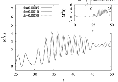
  Figure 18: Dependence of the time evolution of ${\cal M}^{2}(t)$ on the time $\Delta t$ for the simulation with the parameters from Fig. 9 in the time range $t\in[25,50]$; in the inset the whole time range is shown; the momentum distance is fixed at $\Delta p=0.05$ and the momentum cutoff $p_{\mathrm{max}}=10$; the solid line represents the simulation for $\Delta t=0.0005$, the long dashed line $\Delta t=0.001$ and the short dashed line $\Delta t=0.005$.

We would finally like to point out that it is in no way inherent in our numerical approach to use an equidistant momentum grid. Indeed it is more economical to choose $\Delta p$ small for small momenta and to let it increase for larger ones, as was done, .e.g., in previous computations of our group. In one space dimension the choice of equidistant momenta turns momentum conservation in a trivial algebra of indices. In three space dimensions one may use the O$(3)$ invariance of the mode functions as functions of ${\bf p}$. Then, due to angular integrations, the momentum integrals become convolutions of mode functions with phase space functions and an equidistant momentum grid does not lead to any major simplification.

References

- (1) J. Berges, Nucl. Phys. A 699, 847 (2002) [arXiv:hep-ph/0105311].
- (2) G. Aarts, D. Ahrensmeier, R. Baier, J. Berges and J. Serreau, Phys. Rev. D 66, 045008 (2002) [arXiv:hep-ph/0201308].
- (3) J. M. Cornwall, R. Jackiw and E. Tomboulis, Phys. Rev. D 10, 2428 (1974).
- (4) E. Calzetta and B. L. Hu, Phys. Rev. D 35, 495 (1987); Phys. Rev. D 37, 2878 (1988).
- (5) J. S. Schwinger, J. Math. Phys. 2, 407 (1961); L. V. Keldysh, Zh. Eksp. Teor. Fiz. 47, 1515 (1964) [ Sov. Phys. – JETP 20, 1018 (1965)]; see also G. Zhou, Z. Su, B. Hao, and L. Yu, Phys. Rep. 118, 1 (1985).
- (6) B. Mihaila, F. Cooper and J. F. Dawson, Phys. Rev. D 63, 096003 (2001) [arXiv:hep-ph/0006254].
- (7) G. Aarts and J. Berges, Phys. Rev. Lett. 88, 041603 (2002) [arXiv:hep-ph/0107129].
- (8) K. Blagoev, F. Cooper, J. Dawson and B. Mihaila, Phys. Rev. D 64, 125003 (2001) [arXiv:hep-ph/0106195].
- (9) F. Cooper, J. F. Dawson and B. Mihaila, arXiv:hep-ph/0207346.
- (10) J. Berges and J. Cox, Phys. Lett. B 517, 369 (2001) [arXiv:hep-ph/0006160].
- (11) F. Cooper, J. F. Dawson and B. Mihaila, arXiv:hep-ph/0209051.
- (12) J. Berges and J. Serreau, arXiv:hep-ph/0208070.
- (13) J. Baacke and S. Michalski, Phys. Rev. D 65, 065019 (2002) [arXiv:hep-ph/0109137].
- (14) H. Verschelde and M. Coppens, Phys. Lett. B 287, 133 (1992).
- (15) M. Coppens and H. Verschelde, Z. Phys. C 58, 319 (1993).
- (16) H. van Hees and J. Knoll, Phys. Rev. D 65, 025010 (2002) [arXiv:hep-ph/0107200]; Phys. Rev. D 65, 105005 (2002) [arXiv:hep-ph/0111193]; Phys. Rev. D 66, 025028 (2002) [arXiv:hep-ph/0203008].
- (17) H. Verschelde and J. De Pessemier, Eur. Phys. J. C 22, 771 (2002) [arXiv:hep-th/0009241].
- (18) H. Verschelde, Phys. Lett. B 497, 165 (2001) [arXiv:hep-th/0009123].
- (19) G. Smet, T. Vanzielighem, K. Van Acoleyen and H. Verschelde, Phys. Rev. D 65, 045015 (2002) [arXiv:hep-th/0108163].
- (20) J. Baacke and S. Michalski, arXiv:hep-ph/0210060.
- (21) A. Okopinska, Annals Phys. 249, 367 (1996) [arXiv:hep-th/9512113].
- (22) D. Dudal and H. Verschelde, arXiv:hep-th/0210098.
- (23) see, e.g., C. Itzykson and J.-B. Zuber, Quantum field theory, McGraw-Hill Inc., New York 1980, section 1.2.2.
- (24) F. Cooper and E. Mottola, Phys. Rev. D 36, 3114 (1987).
- (25) V. P. Maslov and O. Y. Shvedov, Theor. Math. Phys. 114, 184 (1998) [Teor. Mat. Fiz. 114, 233 (1998)] [arXiv:hep-th/9709151].
- (26) J. Baacke, K. Heitmann and C. Patzold, Phys. Rev. D 57, 6398 (1998) [arXiv:hep-th/9711144].
- (27) C. Destri and E. Manfredini, Phys. Rev. D 62, 025007 (2000) [arXiv:hep-ph/0001177].
- (28) J. H. Traschen and R. H. Brandenberger, Phys. Rev. D 42, 2491 (1990).
- (29) L. Kofman, A. D. Linde and A. A. Starobinsky, Phys. Rev. Lett. 73, 3195 (1994) [arXiv:hep-th/9405187].
- (30) D. Boyanovsky, H. J. de Vega, R. Holman and J. F. Salgado, Phys. Rev. D 54, 7570 (1996) [arXiv:hep-ph/9608205].
- (31) D. Boyanovsky, C. Destri, H. J. de Vega, R. Holman and J. Salgado, Phys. Rev. D 57, 7388 (1998) [arXiv:hep-ph/9711384].
- (32) F. Cooper, S. Habib, Y. Kluger and E. Mottola, Phys. Rev. D 55, 6471 (1997) [arXiv:hep-ph/9610345].
- (33) see, e.g., R. B. Griffiths in Phase Transitions and Critical Phenomena, C. Domb and M.S. Green, Eds., Academic press, New York 1972, Vol. 1, p. 7.
- (34) E. A. Calzetta and B. L. Hu, arXiv:hep-ph/0205271.