$\pi\eta$ scattering in generalized chiral perturbation theory

Abstract

We calculate the amplitude of $\pi\eta$ scattering in generalized chiral perturbation theory at the order $O(p^{4})$ and present a preliminary results for the numerical analysis of the S-wave scattering length, which seems to be particularly sensitive to the deviations from the standard case.

1 Generalized Chiral Perturbation Theory

As it is well known, on the classical level the QCD Lagrangian with $N_{f}$ massless quarks (corresponding to so-called chiral limit of QCD) is invariant w.r.t. chiral symmetry ($\chi S)$ group $SU(N_{f})_{L}\times SU(N_{f})_{R}$. On the quantum level there exist strong theoretical (for $N_{f}\geq 3$) and phenomenological arguments for spontaneous symmetry breakdown (SSB) of $\chi S$ according to the pattern $SU(N_{f})_{L}\times SU(N_{f})_{R}\rightarrow SU(N_{f})_{V}$. As a consequence of Goldstone theorem, $N_{f}^{2}-1$ pseudoscalar Goldstone bosons (GB) appear in the particle spectrum of the theory. These massless pseudoscalars dominate the low energy dynamics of QCD and interact weekly at low energies $E<<\Lambda_{H}$, where $\Lambda_{H}\sim 1GeV$ is the hadronic scale corresponding to the masses of the lightest nongoldstone hadrons. The most important order parameters of this pattern of SSB are the Goldstone boson decay constant $F_{0}$ and the quark condensate $\langle\overline{q_{f}}q_{f}\rangle_{0}$.

Within the real QCD the quark mass term ${\cal L}_{f,mass}^{QCD}\,$breaks $\chi S$ explicitly. The GB become pseudogoldstone bosons (PGB) with nonzero masses. Nevertheless, for $m_{f}<<\Lambda_{H}$, ${\cal L}_{f,mass}^{QCD}$ can be treated as a small perturbation. As a consequence, the PGB masses $M_{P}$ can be expanded in the powers (and logarithms) of the quark masses and the interaction of PGB at energy scale $E<<\Lambda_{H}$ continues to be weak. PGB are identified with $\pi^{0},\pi^{\pm}\,$ for $N_{f}=2$ and $\pi^{0},\pi^{\pm},K^{0},\overline{K^{0}},K^{\pm},\eta$ for $N_{f}=3$. Because $M_{P}<\Lambda_{H}$, the QCD dynamics at $E<<\Lambda_{H}$ is still dominated by these particles and can be described in terms of an effective theory known as chiral perturbation theory ($\chi PT$). The Lagrangian of $\chi PT$ can be constructed on the base of symmetry arguments only; the unknown information about the nonperturbative properties of QCD are hidden in the parameters known as low energy constants (LEC)[1].

In order to be able to treat the effective theory as an expansion in powers of $(p/\Lambda_{H})$ (where $p$ are generic external momenta) and $(m_{f}/\Lambda_{H})$, it is necessary to assign to each term ${\cal L}^{(m,n)}=O(\partial^{m}m_{f}^{n})$ of the effective Lagrangian a single parameter called chiral order. To the terms ${\cal L}_{k}$ with chiral order $k$ it is referred as to $O(p^{k})$ terms. Obviously, $\partial=O(p).$ The matter of discussion is, however, the question concerning the chiral power of $m_{f}$. This question is intimately connected to the scenario according which the SSB of $\chi S$ is realized.

The standard scenario corresponds to the assumption, that the SSB order parameter $\langle\overline{q}q\rangle_{0}$ is large in the sense, that the ratio $X$

$$X=\frac{2B_{0}\widehat{m}}{M_{\pi}^{2}}$$ (1)

(where $B_{0}=-\langle\overline{q}q\rangle_{0}/F_{0}^{2}$ and $\widehat{m}=(m_{u}+m_{d})/2$) is close to one. Because $M_{\pi}^{2}=O(p^{2})$, it is then natural to take $m_{f}=O(p^{2})$, i.e. $k=m+2n$. This results into the Standard $\chi PT$ ($S\chi PT$ in what follows)[2]. This scenario has been experimentally confirmed [3] for $N_{f}=2$ and it is perfectly compatible with experiment for $N_{f}=3$ in $\pi,\,K$ sector.

Let us note that at $O(p^{2})$ there is none free parameter, because at this chiral order $F_{0}=F_{\pi}=93.2{\rm MeV}$, $\,\,2B_{0}\widehat{m}=M_{\pi}^{2}=135{\rm MeV}$ and $r=m_{s}/\widehat{m}\simeq 26$.

Alternative to this way of chiral power counting is Generalized $\chi PT$ ($G\chi PT$) [4] corresponding to the scenario with small quark condensate $X<<1$ so that it is natural to take $m_{f}=O(p)$ and $B_{0}=O(p)$. I.e. $k=m+n$ and the $O(p^{2})$ Lagrangian is

$${\cal L}_{2} = \frac{F_{0}^{2}}{4}\left(\langle\partial_{\mu}U^{+}\partial^{\mu}U\rangle+2B_{0}\langle U^{+}{\cal M}+{\cal M}^{+}U\rangle+A_{0}\langle(U^{+}{\cal M})^{2}+({\cal M}^{+}U)^{2}\rangle\right.$$ (2)

$$+\left.Z_{0}^{P}\langle U^{+}{\cal M}-{\cal M}^{+}U\rangle^{2}+Z_{0}^{S}\langle U^{+}{\cal M}+{\cal M}^{+}U\rangle^{2}\right).$$

This scenario is still possible for $N_{f}=3$, as has been discussed in [5].

In the generalized case, there are two free parameters in the $O(p^{2})$ effective Lagrangian, the usual choice is $(r,\zeta=Z_{0}^{S}/A_{0})$. Within $S\chi PT$ at $O(p^{2})$ we get roughly $(r,\zeta)=(26,0)$. Note, that $\zeta$ measures the violation of Zweig rule in the $0^{++}$ channel, which is, however, not well under control. In what follows, we therefore prefer to parametrize the deviations from $S\chi PT$ directly on terms of $X$, i.e. our choice of free parameters is $(r=m_{s}/\widehat{m},\,\,X)$, cf. (1) (standard $O(p^{2})$ values are then $(26,1)$). The $O(p^{2})$ LEC can be then expressed in terms of these free parameters.

In oder to distinguish between the two scenarios of $\chi S$ SSB, it is necessary to find observables, which are sensitive to the deviations from the standard case. It seems, that the $\pi\eta$ scattering might offer such observables, though we left open the question about their experimental accessibility.

Let us note, that the amplitude of this process was already calculated within $S\chi PT$ to $O(p^{4})$ (and within the extended $S\chi PT$ with explicit resonance fields) in the paper [7], where the authors presented prediction for the scattering lengths and phase shifts of the $S$, $P$ and $D$ partial waves. We quote here their $O(p^{4})$ results for the $S$-wave scattering length $a_{0}$ (in the units of the pion Compton wavelength): $a_{0}^{S\chi PT}=7.3\times 10^{-3}$ and $a_{0}^{S\chi PT+resonances}=4.9\times 10^{-3}$.

2 General structure of the $\pi\eta$ scattering amplitude

Due to isospin conservation and Bose symmetry, the process is described in terms of one $s-u$ symmetric invariant amplitude $A(s,t;u)$

$$\langle\pi^{b}\eta_{out}|\pi^{a}\eta_{in}\rangle={\rm i}(2\pi)^{4}\delta(P_{f}-P_{i})\delta^{ab}A(s,t;u)$$

Using analyticity, unitarity, crossing symmetry and assuming chiral expansion in the same way as in [9] we get the following general form of the $O(p^{4})$ amplitude

$$A(s,t;u) = R^{(3)}(t;s,u)+V_{0}(t)+W_{0}(s)+W_{0}(u)$$ (3)

$$+[(t-u)s+\Delta^{2}]W_{1}(s)+[(t-s)u+\Delta^{2}]W_{1}(u)$$

Here $R^{(3)}(t;s,u)$ is the most general $s-u$ symmetric subtraction polynomial of the third order

$$R^{(3)}(t;s,u) = \frac{1}{3F_{\pi}^{2}}(\alpha_{\pi\eta}M_{\pi}^{2}+\beta_{\pi\eta}(t-\frac{2}{3}\Sigma)+\frac{\lambda_{\pi\eta}}{F_{\pi}^{2}}(t-\frac{2}{3}\Sigma)+\frac{\widetilde{\lambda}_{\pi\eta}}{F_{\pi}^{2}}(s-u)^{2}$$ (4)

$$+\frac{\kappa_{\pi\eta}}{F_{\pi}^{4}}(s-u)^{2}(t-\frac{2}{3}\Sigma)+\frac{\widetilde{\kappa}_{\pi\eta}}{F_{\pi}^{4}}(t-\frac{2}{3}\Sigma)^{3}).$$

The unitarity corrections $V_{0}$,$W_{0}$, $W_{1}$ start at $O(p^{4})$ and are determined by means of the dispersion integrals along the cuts $((M_{\pi}+M_{\eta})^{2},\infty)$ or $(4M_{\pi}^{2},\infty)$ with the discontinuities given by the right hand cut discontinuities of the $S$ and $P$ partial waves in the $s$ and $t$ channel. Using partial waves unitarity, it is possible to proceed iteratively and determine the relevant $O(p^{4})$ discontinuities through the $O(p^{2})$ amplitudes $A^{\eta\pi\rightarrow\phi_{\alpha}\phi_{\beta}}$, $A^{\phi_{\alpha}\phi_{\beta}\rightarrow\eta\pi}$, $A^{\pi\pi\rightarrow\phi_{\alpha}\phi_{\beta}}$ and $A^{\eta\eta\rightarrow\phi_{\alpha}\phi_{\beta}}$. These are real and first order polynomials in $s,\,t,\,u$, so that we can parametrize them with (altogether 11) real parameters. Adding to this the 2 extra real coefficients of $O(p^{4})$ part of the subtraction polynomial $R^{(3)}(t;s,u)$, it is possible to parametrize the $O(p^{4})$ amplitude $A(s,t;u)$ in terms of 13 real free parameters. As a result of the iterative procedure we get for the $O(p^{4})$ unitarity corrections $V_{0}$, $W_{0}$, $W_{1}$ the following formulas: $W_{1}^{(4)}(s)=0$ and

$$W_{0}^{(4)}(s) = \overline{J}_{\pi\eta}(s)\left(\frac{1}{3F_{\pi}^{2}}\alpha_{\pi\eta}M_{\pi}^{2}\right)^{2}$$

$$+\overline{J}_{KK}(s)\frac{3}{8F_{\pi}^{4}}[\beta_{\pi\eta K}(s-\frac{1}{3}\Sigma-\frac{2}{3}M_{K}^{2})-\frac{1}{3}(2M_{K}^{2}-\Sigma+\alpha_{\pi\eta K}M_{\pi}^{2})]^{2}$$

$$V_{0}^{(4)}(s) = \overline{J}_{\pi\pi}(s)\frac{1}{3F_{\pi}^{4}}\alpha_{\pi\eta}M_{\pi}^{2}[\beta_{\pi\pi}(s-\frac{4}{3}M_{\pi}^{2})+\frac{5}{6}\alpha_{\pi\pi}M_{\pi}^{2}]$$

$$-\overline{J}_{\eta\eta}(s)\frac{1}{18F_{\pi}^{4}}\alpha_{\eta\eta}\alpha_{\pi\eta}M_{\pi}^{4}\left(1-\frac{4M_{\eta}^{2}}{M_{\pi}^{2}}\right)$$

$$+\overline{J}_{KK}(s)\frac{1}{8F_{\pi}^{2}}[\beta_{\pi K}(s-\frac{2}{3}M_{\pi}^{2}-\frac{2}{3}M_{K}^{2})+\frac{2}{3}((M_{K}-M_{\pi})^{2}+2\alpha_{\pi K}M_{K}M_{\pi})]$$

$$\times[\beta_{\eta K}(3s-2M_{K}^{2}-2M_{\eta}^{2})+\alpha_{\eta K}(2M_{\eta}^{2}-\frac{2}{3}M_{K}^{2})]$$

where $\overline{J}_{PQ}(s)$ is the Chew-Mandelstam function, cf.[9]. The role of $\chi PT$ is then reduced to the determination of the above mentioned parameters in terms of LEC and quark masses. Let us now briefly comment on the results of the calculations.

3 $\pi\eta$ amplitude in $G\chi PT$ at $O(p^{4})$

Let us write the complete $O(p^{4})$ amplitude $A(s,t,u)$ in the form

$$A(s,t,u)=A^{(2)}(s,t,u)+A^{(3)}(s,t,u)+A^{(4)}(s,t,u),\,\,\,\,\,{\rm where}\,\,\,A^{(k)}(s,t,u)=O(p^{k}).$$

$A^{(2)}$ and $A^{(3)}$ contain the contributions from tree graphs with vertices derived form Lagrangians ${\cal L}_{2}$ and ${\cal L}_{3}=O(p^{3})$ respectively (see (2) and e.g. [8]); $A^{(4)}$ includes tree graphs with vertices from ${\cal L}_{4}=O(p^{4})$ as well as 1-loop graphs with vertices from ${\cal L}_{2}$.

Because the unitarity corrections start at $O(p^{4})$, $A^{(2)}(s,t,u)$ and $A^{(3)}(s,t,u)$ are both polynomials of the form (cf. (4))

$$A^{(k)}(s,t,u)=\frac{1}{3F_{\pi}^{2}}(\alpha_{\pi\eta}^{(k)}M_{\pi}^{2}+\beta_{\pi\eta}^{(k)}(t-\frac{2}{3}(M_{\pi}^{2}+M_{\eta}^{2})),\,\,\,\,\,k=1,2.$$

Moreover, the amplitude must vanish in the chiral limit, therefore $\beta_{\pi\eta}^{(2)}=0$. From (2) we get

$$A^{(2)}(s,t,u)=\frac{M_{\pi}^{2}}{3F_{\pi}^{2}}\alpha_{\pi\eta}^{(2)},$$

where, in terms of the free parameters $(r,X)$

$$\alpha_{\pi\eta}^{(2)}=1+\frac{\,\left(1+2\,r\right)\,\left(2\,\left(1-X\right)+r\varepsilon(r)\right)}{\,\left(2+r\right)}-\frac{2\Delta_{GMO}}{r-1}.$$

In this formula

$$\varepsilon(r)=2\frac{r_{2}-r}{r^{2}-1},\,\,\,r_{2}=2\frac{M_{K}^{2}}{M_{\pi}^{2}}-1,\,\,\,\Delta_{GMO}=\frac{3M_{\eta}^{2}+M_{\pi}^{2}-4M_{K}^{2}}{M_{\pi}^{2}}\simeq-3.6.$$ (5)

The standard $O(p^{2})$ result (corresponding to the current algebra (CA)) corresponds to $\alpha_{\pi\eta}^{(2)}=1$ [7]. The dependence of $\alpha_{\pi\eta}^{(2)}$ on $r$ and $X$ is shown in Fig. 1. The deviation from the standard case might be even by a factor ten larger than the standard value, provided the quark mass ratio $r$ is small in comparison with $r_{2}$ and the three-flavor ratio $X$ is smaller than one. This result is encouraging enough to calculate the higher order corrections.

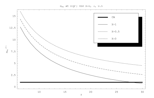
Figure 1: The dependence of the parameter $\alpha_{\pi\eta}^{(2)}$ on $r$ for $X=1,\,\,0.5$ and $0$. The thick solid line corresponds to current algebra result.

The $O(p^{3})$ Lagrangian ${\cal L}_{3}$ contains 9 LEC, namely $\xi$, $\widetilde{\xi}$ and $\rho_{i}$, $i=1,\ldots,7$. $\xi$ can be expressed in terms of decay constants as follows

$$\widehat{m}\xi=\frac{\Delta_{F}}{r-1},\,\,\,\,\,\,\,\Delta_{F}=\frac{F_{K}^{2}}{F_{\pi}^{2}}-1\simeq 0.5.$$

For the NLO corrections in terms of $X$, $\varepsilon$, $\Delta_{GMO}$, $\Delta_{F}$, $\widetilde{\xi}$ and remaining $O(p^{3})$ LEC we get

$$\beta_{\pi\eta}^{(3)} = 4\widehat{m}\widetilde{\xi}(r+2)$$

$$\alpha_{\pi\eta}^{(3)} = \frac{2\Delta_{F}}{(r-1)}(1-\frac{2(2r+1)^{2}(1-X)}{3(r+2)}-\frac{(8+r(6r+13))(r-1)\varepsilon}{6(r+2)}-\frac{\Delta_{GMO}}{3})$$

$$-4\widehat{m}\widetilde{\xi}(2r+1)\left(1-(X-1)+\frac{r^{2}-1}{2r+1}\varepsilon+\frac{\Delta_{GMO}}{2r+1}\right)$$

$$+\frac{8}{3}\widehat{m}\widetilde{\xi}(r+2)\frac{\Sigma}{M_{\pi}^{2}}+\ldots$$

The ellipses stay for the $O(m_{f}^{3})$ terms which includes the unknown LEC $\rho_{i}$.

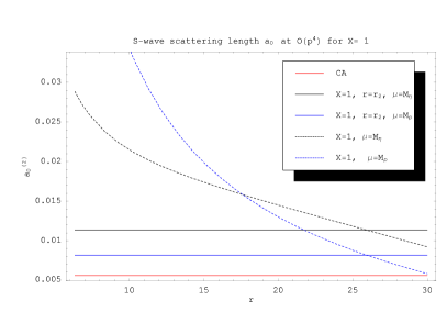
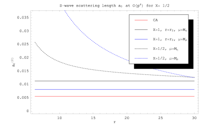
Figure 2: The dependence of the $S$-wave scattering length on $r$ for $X=1$ and $X=0.5$ with $\mu=M_{\eta}$ and $\mu=M_{\rho}$ . The solid lines mimic the $S\chi PT$ ($X=1$ and $r=r_{2}$) at $O(p^{4})$. The lowest line corresponds to current algebra result.

The NNLO $O(p^{4})$ corrections have the general form (cf. (3)) with $\kappa=\widetilde{\kappa}=0$ and   with $V_{0}^{(4)}$ and $W_{i}^{(4)}$ given above. The complete formulas for $A^{(4)}$, which are rather lengthy, will be published elsewhere. Let us only briefly comment on the result.

As usual, 1-loop graphs which contribute to $A^{(4)}$ are generally divergent; therefore the renormalization procedure is needed. As a result, the amplitude depends explicitly on the renormalization scale $\mu$. This scale dependence is compensated by the implicit scale dependence of the renormalized LEC, this fact we used as a nontrivial check of our calculations.

Let us also note, that the $O(p^{4})$ Lagrangian is parametrized by means of 40 LEC, most of them are unknown. Influence of these unknown constant (as well as that of the unknown $O(p^{3})$ LEC) can be roughly estimated using the above mentioned explicite $\mu$ dependence of the amplitude. The idea behind is based on the assumption that the variation of LEC with $\mu$ is of the same order as LEC themselves. Setting all the unknown LEC equal to zero and varying the scale $\mu$ is then (up to the sign) equivalent to the variation of the LEC and gives therefore information on the impact of the unknown LEC.

The observable which seems to be sensitive to the deviation from the $S\chi PT$ is the $S-$wave scattering length $a_{0}$, (note, that at $O(p^{2})$, $a_{0}\propto\alpha_{\pi\eta}^{(2)}$, while $P-$wave scattering length $a_{1}$ starts at $O(p^{3})$ ). In Fig. 2 we show the numerical results for $a_{0}$ as a function of the quark mass ratio $r$ for $X=1$ and $X=0.5\$with $\mu=M_{\eta}$ and $\mu=M_{\rho}$.

4 Conclusions

We have calculated the $\pi\eta$ scattering amplitude in $G\chi PT$ to the order $O(p^{4})$ and evaluated the $S-$wave scattering length as a function of the free parameters $r$ and $X$. The influence of the other unknown LEC was estimated using explicit dependence of the loops on the renormalization scale $\mu$. Preliminary numerical results suggest that $S-$wave scattering length might be sensitive to the values of the quark condensate and quark mass ratio. $G\chi PT$ allows for systematically larger values of $a_{0}$ in comparison to the standard case [7]. The dependence of the loop corrections on the renormalization scale can be understood as a signal for relatively strong dependence on the unknown LEC. In order to get sharper prediction further estimates will be necessary (resonances, sum rules…). Numerical analysis of other observables, which has not been completed yet, might be also interesting.

Acknowledgement. This work was supported by the program “Research Centers” (project number LN00A006) of the Ministry of Education of the Czech Republic.

References

- [1] S. Weinberg, Physica A 96 (1979) 327
- [2] J. Gasser, H. Leutwyler, Annals. Phys 158 (1984) 142, J. Gasser, H. Leutwyler, Nucl. Phys. B250 (1985) 465, 517,539
- [3] S. Pislak et al., BNL-E865 Collaboration, Phys. Rev. Lett. 87 (2001) 221801
- [4] J. Stern, H. Sazdjian, N. H. Fuchs, Phys. Rev. 175 (1991) 183, M. Knecht, B. Moussallam, J. Stern, Nucl. Phys. B429 (1994) 125, M.Knecht, B. Moussallam, J. Stern, N. H. Fuchs, Nucl. Phys. B457 (1995) 513, M.Knecht, B. Moussallam, J. Stern,N. H. Fuchs, Nucl. Phys. B471 (1996) 445
- [5] S. Descotes, J. Stern, Phys. Lett. B488 (2000) 274, S. Descotes, J. High Energy Phys. 0103 (2001) 002, S. Descotes-Genom, L. Girlanda, J. Stern, ArXiv:hep-ph/0207337
- [6] B. Moussallam, Eur. Phys. J. C14 (2000)111, B. Moussallam, J. High Energy Phys. 0008 (2000) 005
- [7] V. Bernard, N. Kaiser, U-G. Meissner, Phys. Rev. D44 (1991) 3698
- [8] M. Knecht, J. Stern, in 2nd DANE Physics Handbook, L. Maiani, G. Pancheri, N. Paver eds., IFNF, Frascati, 1995, p.169
- [9] M.Knecht, B. Moussallam, J. Stern, N. H. Fuchs, Nucl. Phys. B457 (1995) 513