A New 5-Flavour LO Analysis and Parametrization
of Parton Distributions in the Real Photon

Abstract

New, radiatively generated, LO quark ($u,d,s,c,b$) and gluon densities in a real, unpolarized photon are presented. We perform a global 3-parameter fit, based on LO DGLAP evolution equations, to all available data for the structure function $F_{2}^{\gamma}(x,Q^{2})$. We adopt a new theoretical approach called ACOT($\chi$), originally introduced for the proton, to deal with the heavy-quark thresholds. This defines our basic model (CJKL model), which gives a very good description of the experimental data on $F_{2}^{\gamma}(x,Q^{2})$, for both $Q^{2}$ and $x$ dependences. For comparison we perform a standard fit using the Fixed Flavour-Number Scheme (FFNS_CJKL model), updated with respect to the previous fits of this type. We show the superiority of the CJKL fit over the FFNS_CJKL one and other LO fits to the $F_{2}^{\gamma}(x,Q^{2})$ data. The CJKL model gives also the best description of the LEP data on the $Q^{2}$ dependence of the $F_{2}^{\gamma}$, averaged over various $x$-regions, and the $F_{2,c}^{\gamma}$, which were not used directly in the fit. Finally, a simple analytic parametrization of the resulting parton densities obtained with the CJKL model is given.

I Introduction

The photon structure function was recognized as an important quantity already in the early days of the Parton Model zerwas . It has attracted even more attention since the seminal paper by Witten WITTEN , which shows that $F_{2}^{\gamma}$ can serve as a unique test of QCD. This expectation was based on the fact that the (asymptotic) point-like solution of the $Q^{2}$ evolution equation, summing the leading QCD corrections, can be obtained for $F_{2}^{\gamma}$ without additional assumptions. Further studies showed the need of the hadronic, VMD-type, contribution to $F_{2}^{\gamma}$, and consequently the need of an input, as for every other hadronic structure function.

The structure function $F_{2}^{\gamma}$ is extracted from measurements in deep inelastic scattering on a photon target, which can be performed in $e^{+}e^{-}$ experiments. The $F_{2}^{\gamma}$ data are used to construct parametrizations of the parton distributions in the photon. The need for a resolved photon interaction, i.e. where a photon interacts via its partonic agents, has become apparent in other type of processes involving photons, namely in the production of particles with a large transverse momentum. A recent review of the experimental situation and the existing parametrizations can be found in NISIUS .

Our motivation for a new global analysis of the $F_{2}^{\gamma}$ data and for constructing a new parton parametrization for a real unpolarized photon is twofold. On the one hand, there is a vast amount of new experimental data on $F_{2}^{\gamma}(x,Q^{2})$ that has not been used yet to produce the parton parametrizations for the photon. Two recent parametrizations, GRV grv92 and GRS grs , used respectively about 70 and 130 experimental points, while at present a total of 208 independent $F_{2}^{\gamma}(x,Q^{2})$ points exist. On the other hand, there are discrepancies between the theoretical calculations and experimental results for some processes initiated by real photons in which heavy quarks are produced. Let us just mention here the $D^{*}$- and $D_{s}$-meson photoproduction dstar , ds and Frix or the $D^{*}$-meson production with associated dijets dstar at HERA, as examples. The disagreement between the theoretical and experimental results is even more profound for the open beauty-quark production in both HERA bhera and LEP bqOPAL ; bqL3 measurements.

The idea of the radiatively generated parton distributions has been successfully introduced by the GRV group first to describe the parton distributions in the nucleon grvn and pion grvp , and later to create the LO and NLO parton parametrization for the real grv92 and virtual grst photon. Here we follow this approach for a real photon case, limiting ourselves, to the analysis based on the LO QCD. The NLO analysis is under preparation.

As mentioned above there is a problem with the QCD description of heavy-quark production in processes initiated by photons. Therefore, our analysis especially focuses on the heavy-quark contributions to the $F_{2}^{\gamma}(x,Q^{2})$. We apply a new Variable Flavour-Number Scheme (VFNS) approach, denoted by ACOT($\chi$), proposed for heavy-quark production in the $ep$ collision (“electroproduction”) in tung . For comparison we perform a standard Fixed Flavour-Number Scheme (FFNS) fit as well. Since these two approaches are based on very distinct schemes, and since they need different evolution programs, we will refer to them as to two models, CJKL (ACOT($\chi$) type) and FFNS_CJKL models, respectively.

Our paper is divided into six parts. In section 2 we describe various approaches including the ACOT($\chi$) scheme tung , applied to the production of heavy quarks in hadronic processes. Section 3 is devoted to the description of the $F_{2}^{\gamma}$ in LO QCD, paying special attention to an implementation of the ACOT($\chi$) scheme in the calculation of the $F_{2}^{\gamma}(x,Q^{2})$. In section 4 a description of the two global fits performed by us is given. In particular, we present the solutions of the DGLAP evolution in both models. We describe in detail the assumptions for the input parton densities. In the fifth section of the paper, the results of the global fits are discussed and compared with the data for the $F_{2}^{\gamma}(x,Q^{2})$, and for the $F_{2}^{\gamma}(x,Q^{2})$ averaged over various $x$-regions. A comparison with LEP data for $F_{2,c}^{\gamma}$ is presented in section 5 as well. The summary of the paper and an outlook of work in progress can be found in section 6. Finally, in the appendix we give a simple parametrization of the CJKL (LO) parton distributions.

II Various schemes for a description of heavy-quarks production: the proton-target case

In this section we describe various schemes, which are used in the calculation of the heavy-quark production in hadronic processes. There exist two standard schemes. In the FFNS, the light quarks ($u,d$ and $s$) and the heavy ones ($c$ and $b$) are treated on a different footing. The light ones are treated as being massless, and together with the gluons, are the only partons in the proton. The massive charm- and beauty-quarks are produced in the hard subprocesses: they can only appear in the final state of the process. In the second scheme, the Zero-mass Variable Flavour-Number Scheme (ZVFNS), when the characteristic hard scale of the process is larger than some threshold associated with a heavy quark, this quark is also considered as a massless parton in the proton, in addition to the three light quarks. In this way, the number of different types of quarks (flavours) that we treat as partons in the proton increases with the scale of the process.

For the Deep Inelastic Scattering on the proton (DIS_ep), where the structure functions of the proton are measured, the condition for considering a heavy quark to be a parton of the proton is given by a simple (kinematic) threshold condition for the total energy in the $\gamma^{*}p$ collision $W$, namely $W>2m_{h}$ (from now on we will denote the heavy quarks by $h$). It defines the kinematically allowed region for the production of a heavy-quark pair. However, for the structure functions, e.g. $F_{2}^{p}(x,Q^{2})$, and further for the parton densities $q^{p}(x,Q^{2})$, not $W$ but the virtuality of the probing photon $Q^{2}$ is considered to be a natural scale. In the inclusive production of heavy quarks, their transverse momentum or mass is often taken as a characteristic (hard) scale $\mu$, where $\mu\gg\Lambda_{QCD}$, at which parton densities of the initial hadrons are probed. The two, massive and massless, approaches are considered to be reliable in different $\mu$ regions. The FFNS loses its descriptive power when $\mu\gg m_{h}$; on the other hand the ZVFNS does not seem appropriate if $\mu\approx m_{h}$. In order to achieve a prescription working in all hard scale regions, various schemes trying to combine the two approaches have been proposed. They have a generic name: Variable Flavour-Number Schemes (VFNSs). The first of such approaches was introduced by the ACOT group in acot . Other groups, such as RT rth , BMSN bmsn or CSN csnc , created their own versions of the VFNS.

Let us discuss some aspects of the VFNS in more detail. The VFNS introduce the notion of “active quarks”, for which the condition $\mu>m_{q}$ is fulfilled. Such quarks can be treated as (massless) partons of the initial hadron(s). Light ($u,d$ and $s$) quarks are always active because for them $\mu\gg\Lambda_{QCD}\geq m_{q}$. The heavy-quark densities vanish for $\mu\leq m_{h}$, otherwise they differ from zero like in the ZVFNS. For example, for the charm quark we see that at $\mu=m_{c}$ we turn from a Three Flavour-Number Scheme to a Four Flavour-Number one. If $N_{f}$ equals the number of active (massless) quarks, we define the $N_{f}$-FNS as one where the $N_{f}$ first quarks are treated as light and the remaining quarks as heavy.

In calculations based on the VFNS we take into account the sum of all contributions, which would be included separately in the ZVFNS and FFNS. Such procedure requires a proper subtraction of the double-counted contributions. Such contributions have the form of the large logarithms $\ln\mu^{2}$, and are already resummed in the density $q_{h}(x,\mu^{2})$.

An important aspect of the VFNS is the behaviour of the heavy-quark contributions in the threshold region. Let us discuss as an example the production of heavy quarks in DIS_ep. As was already mentioned, a heavy quark can be considered as a parton of the proton if the centre of mass energy of the hard process is $W>2m_{h}$. However, if we use $\mu^{2}$ equal to $Q^{2}$, where $Q^{2}=W^{2}\frac{x}{1-x}$, and impose the threshold condition on $\mu^{2}$, then, for any $Q^{2}$, it may happen (for small enough $x$) that $q_{h}(x,Q^{2})=0$ in the kinematically allowed region, i.e. for $W>2m_{h}$. On the other hand, non-zero heavy-quark densities may appear in the kinematically forbidden region in the ($x,Q^{2}$) plane. Moreover, such conditions can lead to a very steep or even non-continuous growth of the heavy-quark distributions at the threshold.

In general one should ensure that all the ZVFNSs and relevant subtraction terms smoothly vanish when $W\to 2m_{h}$. Then, the non-zero contributions should give only those terms which arise in the FFNS approach, since this approach should reliably describe the region $W\approx 2m_{h}$. Different threshold conditions were used in different analyses; in particular, the ACOT group proposed to use a variable $\mu^{2}$ given by

$$\mu^{2}=\begin{cases}m_{h}^{2}+cQ^{2}(1-m_{h}^{2}/Q^{2})^{n}&\mathrm{for}\quad Q^{2}>m_{h}^{2},\\ m_{h}^{2}&\mathrm{for}\quad Q^{2}\leq m_{h}^{2},\end{cases}$$ (1)

where $c=0.5$ and $n=2$ in acot . Still, in their approach the heavy-quark densities satisfy the boundary condition at $Q^{2}=m_{h}^{2}$

$$q_{h}(x,\mu^{2})\begin{cases}=0&\mathrm{for}\quad\mu^{2}=m_{h}^{2}\quad(Q^{2}\leq m_{h}^{2}),\\ \neq 0&\mathrm{for}\quad\mu^{2}>m_{h}^{2}\quad(Q^{2}>m_{h}^{2}).\end{cases}$$ (2)

Recently, a purely kinematic solution of the threshold-behaviour problem has been found, on which the so-called ACOT($\chi$) scheme tung is based. A new variable, $\chi_{h}\equiv x(1+4m_{h}^{2}/Q^{2})$, has been introduced to replace the Bjorken $x$ as an argument in the heavy-quark $h$ density in the ZVFNS contributions. More details can be found in section 3.

Although the above discussion was focused on the proton case, the problems with the proper treatment of the heavy-quark thresholds in the parton distribution are very similar for any target. In this paper we adopt the ACOT($\chi$) scheme to the real photon case for the very first time.

III Description of $F_{2}^{\gamma}$ in the ACOT($\chi$) scheme

In this section we first recall the basic facts related to the structure function $F_{2}^{\gamma}(x,Q^{2})$ for the real photon. Then we introduce the ACOT($\chi$) approach for the photonic case.

III.1 The parton densities in the photon

The Deep Inelastic Scattering on a real photon (DIS_eγ) allows us to measure the structure function $F_{2}^{\gamma}$, and also other structure functions, $F_{1}^{\gamma}$, $F_{L}^{\gamma}$, $\cdots$, via the process

$$\gamma^{*}\gamma\rightarrow\mathrm{hadrons},$$ (3)

see [1–3]. In the Parton Model this is described at lowest order by the Bethe–Heitler (BH) process, $\gamma^{*}\gamma\to q\bar{q}$ (see Fig. 1).

In the leading logarithmic ($\ln Q^{2}$) approximation or, in short, in the leading order of QCD (LO QCD), the photon structure function $F_{2}^{\gamma}(x,Q^{2})$ can be written in terms of quark (antiquark) densities $q_{i}^{\gamma}(\bar{q}_{i}^{\gamma})$ as follows

$$\frac{1}{x}F_{2}^{\gamma}(x,Q^{2})=\sum_{i=1}^{N_{f}}e_{i}^{2}(q_{i}^{\gamma}+\bar{q}_{i}^{\gamma})(x,Q^{2}),$$ (4)

where $N_{f}$ is the number of different quark flavours, that can appear in the photon (“active quarks”). Note that $q_{i}^{\gamma}(x,Q^{2})=\bar{q}_{i}^{\gamma}(x,Q^{2})$.

The evolution of the parton densities with $\ln Q^{2}$ is governed by the inhomogeneous DGLAP equations. In LO we have for a quark (similarly for an antiquark) and a gluon density

$$\frac{dq_{i}^{\gamma}(x,Q^{2})}{d\ln Q^{2}} = \frac{\alpha}{2\pi}e_{i}^{2}k(x)+\frac{\alpha_{s}(Q^{2})}{2\pi}\int_{x}^{1}\frac{dy}{y}\Bigg{[}P_{qq}\left(\frac{x}{y}\right)q_{i}^{\gamma}(y,Q^{2})+P_{qG}\left(\frac{x}{y}\right)G^{\gamma}(y,Q^{2})\Bigg{]},$$ (5)

$$\frac{dG^{\gamma}(x,Q^{2})}{d\ln Q^{2}} = \frac{\alpha_{s}(Q^{2})}{2\pi}\int_{x}^{1}\frac{dy}{y}\Bigg{[}P_{Gq}\left(\frac{x}{y}\right)\sum_{i=1}^{N_{f}}(q_{i}^{\gamma}+\bar{q}_{i}^{\gamma})(y,Q^{2})+P_{GG}\left(\frac{x}{y}\right)G^{\gamma}(y,Q^{2})\Bigg{]}.$$ (6)

The $k(x)$ term on the right-hand side of Eq. (5) comes from the Bethe–Heitler process of Fig. 1; for 3 colours we have

$$k(x)=3\left[x^{2}+(1-x)^{2}\right].$$ (7)

The functions $P_{i}(x)$ are the LO splitting functions ap

$$\begin{split}P_{qq}(x)&=\frac{4}{3}\left[\frac{1+x^{2}}{(1-x)_{+}}+\frac{3}{2}\delta(1-x)\right],\\ P_{qG}(x)&=\frac{1}{2}\left[x^{2}+(1-x)^{2}\right],\\ P_{Gq}(x)&=\frac{4}{3}~{}\frac{1+(1-x)^{2}}{x},\\ P_{GG}(x)&=6\left[\frac{x}{(1-x)_{+}}+\frac{1-x}{x}+x(1-x)\right]+\left[\frac{11}{2}-\frac{N_{f}}{3}\right]\delta(1-x).\end{split}$$ (8)

Note that the function $k(x)$ describes a photon into quark splitting, so one has $k(x)\equiv P_{q\gamma}(x)$.

III.1.1 Heavy-quark contributions to $F_{2}^{\gamma}$ in the FFNS

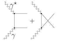
Figure 1: The Bethe–Heitler process $\gamma^{*}\gamma\rightarrow q\bar{q}$.

The standard FFNS approach corresponds to a number of “active quarks” ($N_{f}$) =3, so only the light quarks (and their antiquarks) are taken into account in the sum in Eq. (4). The main heavy-quark contributions to $F_{2}^{\gamma}$ are obtained in this scheme from the corresponding Bethe–Heitler process (Fig. 1 with $q\rightarrow h$)

$$\gamma^{\star}\gamma\to h\bar{h},$$ (9)

keeping the heavy-quark masses in the calculation. It reads

$$\frac{1}{x}F_{2,h}^{\gamma}(x,Q^{2})|_{\mathrm{dir}}=3\frac{\alpha}{\pi}e_{h}^{4}\omega(x,Q^{2}),$$ (10)

with

$$\omega(x,Q^{2}) = \beta\bigg{[}-1+8x(1-x)-x(1-x)\frac{4m_{h}^{2}}{Q^{2}}\bigg{]}$$ (11)

$$+\ln\left(\frac{1+\beta}{1-\beta}\right)\bigg{[}x^{2}+(1-x)^{2}+x(1-3x)\frac{4m_{h}^{2}}{Q^{2}}-x^{2}\frac{8m_{h}^{4}}{Q^{4}}\bigg{]}$$

$$\beta = \sqrt{1-\frac{4m_{h}^{2}x}{(1-x)Q^{2}}}=\sqrt{1-\frac{4m_{h}^{2}}{W^{2}}}.$$ (12)

We call this contribution $F_{2,h}^{\gamma}|_{\mathrm{dir}}$ since here the real photon (i.e. the target photon) interacts directly. However, there exists another heavy-quark contribution, related this time to the process with the resolved initial photon, namely

$$\gamma^{\star}G^{\gamma}\to h\bar{h},$$ (13)

with a gluonic parton of the photon target (as in Fig. 1 with $\gamma\to G^{\gamma}$); it gives

$$F_{2,h}^{\gamma}(x,Q^{2})|_{\mathrm{res}}=\frac{\alpha_{s}(Q^{2})}{2\pi}e_{h}^{2}\int_{\chi_{h}}^{1}\!\frac{x}{z}\omega\!\left(\frac{x}{z},Q^{2}\right)G^{\gamma}(z,Q^{2})dz,$$ (14)

where

$$\chi_{h}\equiv x\left(1+\frac{4m_{h}^{2}}{Q^{2}}\right).$$ (15)

III.1.2 Heavy-quark contributions to $F_{2}^{\gamma}$ in the ZVFNS

In the ZVFNS, the number of “active quarks” changes with the hard scale, as described in the previous section. For low scales the sum in Eq. (4) extends to $N_{f}=3$ but whenever a heavy quark threshold is surpassed the value of $N_{f}$ is increased by 1. It is worth mentioning that in some parton parametrizations for a real photon the heavy-quark densities do appear; however they are described in the threshold region $W\approx 2m_{h}$ only by the above Bethe–Heitler formula (Eqs. (10) and (11)). Moreover, instead of the restriction on $W$ one sometimes takes a (reasonable) condition on $Q^{2}$ (see, for instance, the GS parametrization  gs ). Of course well above a heavy-quark threshold, such a quark can be included among the active (massless) quarks and then $N_{f}\to N_{f}+1$, see e.g. grvp .

III.2 ACOT($\chi$) scheme for $F_{2}^{\gamma}$

The ACOT($\chi$) prescription combines the FFNS and ZVFNS, so that we have to add all relevant contributions from both approaches. For the light-quark contributions we take the form given in Eq. (4) with $N_{f}=3$, while for the heavy quarks we include the following terms:

$$\tilde{F}_{2}^{\gamma}(x,Q^{2})|_{c,b} = \sum_{h(=c,b)}^{2}\big{[}xe_{h}^{2}(q_{h}^{\gamma}+\bar{q}_{h}^{\gamma})(x,Q^{2})+F_{2,h}^{\gamma}(x,Q^{2})|_{\mathrm{dir}}+F_{2,h}^{\gamma}(x,Q^{2})|_{\mathrm{res}}\big{]},\qquad$$ (16)

where $F_{2,h}^{\gamma}(x,Q^{2})|_{\mathrm{dir}}$ and $F_{2,h}^{\gamma}(x,Q^{2})|_{\mathrm{res}}$ are given in Eqs. (10) and (14), respectively.

In Eq. (16) we double-count some heavy-quark contributions. Indeed, part of the $F_{2,h}^{\gamma}|_{\mathrm{dir}}$ contribution from $\gamma^{\star}\gamma\to h\bar{h}$ corresponds to the collinear configuration. Such a configuration leads to a contribution proportional to $\ln Q^{2}$ and is already included in the DGLAP equation for $q^{\gamma}_{h}(x,Q^{2})$, via the $k(x)$ term. Therefore we must subtract from (16) the following terms

$$F_{2,h}^{\gamma}|_{\mathrm{dir},\mathrm{subtr}}=x\ln\frac{Q^{2}}{m_{h}^{2}}3e_{h}^{4}\frac{\alpha}{\pi}\left(x^{2}+(1-x)^{2}\right),$$ (17)

coming from an exact solution of a part of the DGLAP equation, namely

$$\frac{dq_{h}^{\gamma}(x,Q^{2})}{d\ln Q^{2}}=\frac{\alpha}{2\pi}e_{h}^{2}k(x),$$ (18)

integrated over the $Q^{2}$ from $m_{h}^{2}$ to $Q^{2}$.

Similarly, $F_{2,h}^{\gamma}|_{\mathrm{res}}$ from the $\gamma^{\star}G^{\gamma}\to h\bar{h}$ process, has a $\ln Q^{2}$ part that corresponds to the collinear configuration already included in the DGLAP equation for $q^{\gamma}_{h}(x,Q^{2})$, via the $P_{qG}\left(\frac{x}{y}\right)G^{\gamma}(y,Q^{2})$ term. The term to be subtracted reads, in this case:

$$F_{2,h}^{\gamma}|_{\mathrm{res},\mathrm{subtr}}=\>x\ln\left(\frac{Q^{2}}{m_{h}^{2}}\right)e_{h}^{2}\frac{\alpha_{s}(Q^{2})}{\pi}\int_{x}^{1}\frac{dy}{y}P_{qG}\left(\frac{x}{y}\right)G^{\gamma}(y,Q^{2}).$$ (19)

It is based on an approximated solution for the other part of Eq. (5), namely

$$\frac{dq_{h}^{\gamma}(x,Q^{2})}{d\ln Q^{2}}=\frac{\alpha_{s}(Q^{2})}{2\pi}\int_{x}^{1}\frac{dy}{y}\left[P_{qG}\left(\frac{x}{y}\right)G^{\gamma}(y,Q^{2})\right].$$ (20)

The solution (19) is obtained by the integration of Eq. (20) over the same $Q^{2}$ region as above, after neglecting the $Q^{2}$ dependence of $\alpha_{s}$ and $G^{\gamma}$. The final subtraction term is

$$F_{2}^{\gamma}(x,Q^{2})|_{\mathrm{subtr};c,b}=\!\sum_{h(=c,b)}^{2}\!\big{[}F_{2,h}^{\gamma}|_{\mathrm{dir},\mathrm{subtr}}+F_{2,h}^{\gamma}|_{\mathrm{res},\mathrm{subtr}}\big{]}.$$ (21)

So, finally we have, for heavy-quarks: $F_{2}^{\gamma}(x,Q^{2})|_{c,b}=\tilde{F}_{2}^{\gamma}(x,Q^{2})|_{c,b}-F_{2}^{\gamma}(x,Q^{2})|_{\mathrm{subtr};c,b}$. A graphical representation of all terms included in the analysis, Eqs. (16) and (21), is presented in Fig. 2.

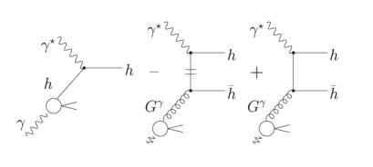
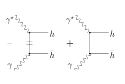
Figure 2: Graphical representation of the ACOT model for $F_{2}^{\gamma}$. The first diagram represents the ZVFNS contribution. The third (fifth) diagram shows the FFNS contribution of the resolved (direct) photon, while the second (fourth) diagram is the corresponding subtraction term.

Further, we need to ensure that all terms containing the heavy-quark $h$ disappear when $W\to 2m_{h}$. The FFNS contributions, $F_{2,h}^{\gamma}|_{\mathrm{dir}}$ (Eqs. (10–12)) and $F_{2,h}^{\gamma}|_{\mathrm{res}}$ (Eqs. (14),(15)), behave properly at the thresholds. The problem emerges for the heavy-quark densities $q_{h}^{\gamma}$ and the subtraction terms (Eqs. (18),(19)). These terms do not naturally disappear for $W\to 2m_{h}$. Fortunately, this problem can be cured; we noticed that the resolved-photon contribution in Eq. (14) vanishes for $W\to 2m_{h}$ because then $\chi_{h}\to 1$ and the corresponding integral disappears. So, we can do the same with the $q_{h}^{\gamma}$ distribution and the subtraction terms, if instead of $x$ we introduce the $\chi_{h}$ variable (Eq. (15)) slightly shifted from $x$. This way we force the heavy-quark distribution and the second term of the subtraction contribution (the integral term) to vanish at the corresponding threshold. Unfortunately, unlike for the proton, in the case of the photon we are left with the $F_{2,h}^{\gamma}|_{\mathrm{dir},\mathrm{subtr}}$ contribution, which is now proportional to $\chi_{h}^{2}+(1-\chi_{h})^{2}$ and does not vanish for $\chi_{h}\to 1$. In the large-$Q^{2}$ region, where the ZVFNS is reliable, this change of variables is irrelevant. In the numerical calculations we ensure that the total contributions to $F_{2}^{\gamma}$ due to heavy quarks are not negative (positivity constraint). This way we effectively introduce small additional terms near the charm- and beauty-quark thresholds. The final formula for the $F_{2}^{\gamma}(x,Q^{2})$ in the ACOT$(\chi)$ scheme reads

$$F_{2}^{\gamma}(x,Q^{2}) = \sum_{i=1}^{3}xe_{i}^{2}(q_{i}^{\gamma}+\bar{q}_{i}^{\gamma})(x,Q^{2})+\sum_{h(=c,b)}^{2}xe_{h}^{2}(q_{h}^{\gamma}+\bar{q}_{h}^{\gamma})(\chi_{h},Q^{2})$$

$$+\sum_{h(=c,b)}^{2}\left[F_{2,h}^{\gamma}(x,Q^{2})|_{\mathrm{dir}}+F_{2,h}^{\gamma}(x,Q^{2})|_{\mathrm{res}}\right]$$

$$-\sum_{h(=c,b)}^{2}x\ln\frac{Q^{2}}{m_{h}^{2}}\left[e_{h}^{4}\frac{\alpha}{\pi}k(\chi_{h})+e_{h}^{2}\frac{\alpha_{s}(Q^{2})}{\pi}\int_{\chi_{h}}^{1}\frac{dy}{y}P_{qG}\left(\frac{\chi_{h}}{y}\right)G^{\gamma}(y,Q^{2})\right].$$

As can be seen the heavy-quark distributions are included in the second sum as $q_{h}^{\gamma}(\chi_{h},Q^{2})$, being $\chi_{h}$ functions of $x$ (and $Q^{2}$). We parametrize the final form obtained for these distributions in the Appendix as simple functions of $x$ and $Q^{2}$.

The $\chi_{h}$ variables of the ACOT($\chi$) scheme recall the so-called “slow rescaling” obtained in early papers on the charm-quark production in the DIS_ep (e.g. slowresc ), where the Bjorken $x$ was replaced with $\zeta$:

$$x\to\zeta=x\left(1+\frac{m_{c}^{2}}{Q^{2}}\right).$$ (23)

IV Global fits - solving the DGLAP evolution

Using all the existing $F_{2}^{\gamma}(x,Q^{2})$ data we perform two global fits, both based on the LO DGLAP evolution equations. One fit uses the ACOT$(\chi)$, the other a FFNS model for the heavy-quark contributions.

First we introduce the basic ingredients that are common for the two considered models.

IV.1 Mellin moments

The LO DGLAP evolution equations are very much simplified if they are transformed into the Mellin-moments space. The $n$-th moment for the quark or gluon densities, $f_{i}^{\gamma}$, is defined by

$$f_{i}^{\gamma,n}(Q^{2})=\int_{0}^{1}x^{n-1}f_{i}^{\gamma,n}(x,Q^{2})dx.$$ (24)

Analogous definitions can be used for the splitting functions $P_{ij}^{n}$. The evolution equations in the Mellin space have the generic form

$$\frac{df_{i}^{\gamma,n}(Q^{2})}{d\ln Q^{2}}=\frac{\alpha}{2\pi}k_{i}^{n}(x)+\frac{\alpha_{s}(Q^{2})}{2\pi}P_{ij}^{n}f_{j}^{\gamma,n}(Q^{2}).$$ (25)

Obviously, the first term on the right-hand side appears only for the quark densities. For simplicity, in the following we will skip all subscripts and superscripts wherever possible.

IV.2 Non-singlet and singlet parton densities

To solve the DGLAP equations we need to decompose the parton densities into the singlet and non-singlet (in flavour space) combinations. For the non-singlet (ns) case we have

$$\begin{split}f_{\mathrm{ns}_{N_{f}}}^{\gamma}(Q^{2})=\;&\sum_{i=1}^{N_{f}}(e_{i}^{2}-\langle e^{2}\rangle)\left[q_{i}^{\gamma}(Q^{2})+\bar{q}_{i}^{\gamma}(Q^{2})\right],\\ k_{\mathrm{ns}_{N_{f}}}=\;&2N_{f}\left(\langle e^{4}\rangle-{\langle e^{2}\rangle}^{2}\right)k\end{split}$$ (26)

where

$$\langle e^{k}\rangle\;=\;N_{f}^{-1}\sum_{i=1}^{N_{f}}e_{i}^{k}$$ (27)

and $e_{i}$ stands for the corresponding quark electric charge. Similarly for the singlet (s) densities we have

$$\begin{split}f_{\mathrm{s}}^{\gamma}(Q^{2})\;=\;&\left[\begin{array}[]{c}\Sigma^{\gamma}(Q^{2})\\ G^{\gamma}(Q^{2})\end{array}\right],\\ \Sigma^{\gamma}(Q^{2})\;=\;&\sum_{i=1}^{N_{f}}[q_{i}^{\gamma}(Q^{2})+\bar{q}_{i}^{\gamma}(Q^{2})].\qquad\qquad\!\end{split}$$ (28)

In the singlet case the DGLAP equations (25) become a matrix equation with

$$\hat{P}=\left[\begin{array}[]{cc}P_{qq}&2N_{f}P_{qG}\\ P_{Gq}&P_{GG}\end{array}\right],\qquad\hat{k}=\left[\begin{array}[]{c}k_{\mathrm{s}}\\ 0\end{array}\right]$$ (29)

with

$$k_{\mathrm{s}}=2N_{f}\langle e^{2}\rangle k.$$ (30)

IV.3 Point- and hadron-like parts

The solution of the DGLAP equations can be divided into the so-called point-like (pl) part, related to a special solution of the full inhomogeneous equation and hadron-like (had) part, arising as a general solution of the homogeneous equation. Their sum gives the partonic density in the photon, so we have

$$f^{\gamma}(Q^{2})=f_{\mathrm{had}}^{\gamma}(Q^{2})+f_{\mathrm{pl}}^{\gamma}(Q^{2})$$ (31)

where

$$f_{\mathrm{pl}}^{\gamma}(Q^{2}) = \frac{4\pi}{\alpha_{s}(Q^{2})}\frac{1}{1-2P/\beta_{0}}\frac{\alpha}{2\pi\beta_{0}}\left[1-L^{1-2P/\beta_{0}}\right]k,$$

(32)

$$f_{\mathrm{had}}(Q^{2}) = L^{-2P/\beta_{0}}f^{\gamma}(Q_{0}^{2}).$$

Here $\beta_{0}=11-2N_{f}/3$, $P$ equals $P_{qq}$ ($\hat{P}$) for the non-singlet (singlet) parton densities, and $L=\frac{\alpha_{s}(Q^{2})}{\alpha_{s}(Q_{0}^{2})}$, where the $Q_{0}^{2}$ is the evolution starting (input) scale. Note that at $Q^{2}=Q_{0}^{2}$ the point-like part vanishes.

IV.4 Input parton densities. VMD

Following grv92 , the input scale has been chosen to be small, $Q_{0}^{2}=0.25$ GeV², hence our parton densities are radiatively generated. The point-like contributions are given by Eq. (30), while the hadronic parts need the input distributions. For this purpose we utilize the Vector Meson Dominance (VMD) model VMD , where

$$f_{\mathrm{had}}^{\gamma}(x,Q_{0}^{2})=\sum_{V}\frac{4\pi\alpha}{\hat{f}^{2}_{V}}f^{V}(x,Q_{0}^{2}),$$ (33)

with the sum running over all light vector mesons (V) into which the photon can fluctuate. The parameters $\hat{f}^{2}_{V}$ can be extracted from the experimental data on the $\Gamma(V\to e^{+}e^{-})$ width. In practice one takes into account the $\rho^{0}$ meson and the contributions from other mesons are accounted for via a parameter $\kappa$, which is left as a free parameter. We take

$$f_{\mathrm{had}}^{\gamma}(x,Q_{0}^{2})=\kappa\frac{4\pi\alpha}{\hat{f}^{2}_{\rho}}f^{\rho}(x,Q_{0}^{2}).$$ (34)

In the GRV prescription grv92 the parton densities in the $\rho^{0}$ meson are approximated by the pionic ones: $f^{\rho}(x,Q^{2}_{0})\approx f^{\pi}(x,Q^{2}_{0})$. However, this assumption ignores among others the possible effects of the pseudo-Goldstone boson nature of the pion, and we are not using it in our analysis. Instead we use the input densities of the $\rho^{0}$ meson at $Q_{0}^{2}=0.25$ GeV² in the form of valence-like distributions both for the (light) quark ($v^{\rho}$) and gluon ($G^{\rho}$) densities. All sea-quark distributions (denoted by $\zeta^{\rho}$) are neglected at the input scale. At this scale, the densities $v^{\rho},G^{\rho}$ and $\zeta^{\rho}$ are related, according to Eq. (34) to the corresponding densities for a photon; see below.

The $v^{\rho}$ density is given by

$$v^{\rho}(x,Q_{0}^{2})=\frac{1}{4}(u^{\rho^{+}}+\bar{u}^{\rho^{-}}+d^{\rho^{-}}+\bar{d}^{\rho^{+}})(x,Q_{0}^{2}),$$ (35)

where from the isospin symmetry

$$u^{\rho^{+}}(x,Q_{0}^{2})=\bar{u}^{\rho^{-}}(x,Q_{0}^{2})=d^{\rho^{-}}(x,Q_{0}^{2})=\bar{d}^{\rho^{+}}(x,Q_{0}^{2}).$$ (36)

Note that all the densities in Eq. (35) are normalized to 1, i.e. $\int^{1}_{0}u^{\rho^{+}}dx=1$.

The following constraints should hold for the $v^{\rho}(x,Q_{0}^{2})$ density. The first is related to a number of valence quarks in the $\rho^{0}$ meson, and we have

$$\int_{0}^{1}2v^{\rho}(x,Q_{0}^{2})dx=2.$$ (37)

The second constraint represents the energy-momentum sum rule

$$\int_{0}^{1}x\left(2v^{\rho}(x,Q_{0}^{2})+G^{\rho}(x,Q_{0}^{2})\right)dx=1.$$ (38)

We parametrize the input densities as follows

$$x\zeta^{\rho}(x,Q_{0}^{2}) = 0,$$ (39)

$$xv^{\rho}(x,Q_{0}^{2}) = N_{v}x^{\alpha}(1-x)^{\beta},$$ (40)

$$xG^{\rho}(x,Q_{0}^{2}) = \tilde{N}_{g}xv^{\rho}(x,Q_{0}^{2})=N_{g}x^{\alpha}(1-x)^{\beta},$$ (41)

where $N_{g}=\tilde{N}_{g}N_{v}$, and impose two constraints given by Eqs. (37) and (38) in both models. These constraints allow us to express the normalization factors $N_{v}$ and $N_{g}$ as functions of $\alpha,\beta$ and $\kappa$. This leaves these three parameters as the only free parameters to be fixed in the fits to the $F_{2}^{\gamma}$ experimental data.

IV.5 FFNS_CJKL model

In the FFNS_CJKL model the number of “active quarks” ($N_{f}$) equals 3, so $\langle e^{2}\rangle=2/9$.

To describe the hadron-like part of the solution of DGLAP equations for the photon, we introduce, apart from the valence-like quark and gluon densities, also the sea distribution $\zeta_{\mathrm{had}}^{\gamma}(x,Q^{2})$. The up-, down- and strange-quark densities in the photon are then given by the following combinations

$$u_{\mathrm{had}}^{\gamma}(x,Q^{2}) = d_{\mathrm{had}}^{\gamma}(x,Q^{2})=\frac{1}{2}\left[v_{\mathrm{had}}^{\gamma}(x,Q^{2})+2\zeta_{\mathrm{had}}^{\gamma}(x,Q^{2})\right],$$ (42)

$$s_{\mathrm{had}}^{\gamma}(x,Q^{2}) = \zeta_{\mathrm{had}}^{\gamma}(x,Q^{2}).$$ (43)

¿From Eqs. (26) and (28) we get (below we simply use $f_{\mathrm{ns}}^{\gamma}$ instead of $f_{\mathrm{ns}_{3}}^{\gamma}$):

$$f_{\mathrm{ns},\mathrm{had}}^{\gamma}(x,Q^{2}) = \!\frac{1}{9}v_{\mathrm{had}}^{\gamma}(x,Q^{2}),$$ (44)

$$\Sigma_{\mathrm{had}}^{\gamma}(x,Q^{2}) = 2v_{\mathrm{had}}^{\gamma}(x,Q^{2})+6\zeta_{\mathrm{had}}^{\gamma}(x,Q^{2}).$$ (45)

After performing the DGLAP evolution of $f_{\mathrm{ns},\mathrm{had}}^{\gamma}(x,Q^{2})$ and $\Sigma_{\mathrm{had}}^{\gamma}(x,Q^{2})$ from $Q_{0}^{2}$ to higher $Q^{2}$, we calculate $v_{\mathrm{had}}^{\gamma}(x,Q^{2})$ and $\zeta_{\mathrm{had}}^{\gamma}(x,Q^{2})$. Finally, using formulae (42) and (43), we obtain the hadron-like part for the individual quark densities.

As the down- and strange-quarks have equal electric charges, there are only two different point-like distributions: $u_{\mathrm{pl}}^{\gamma}(x,Q^{2})$ and $d_{\mathrm{pl}}^{\gamma}(x,Q^{2})=s_{\mathrm{pl}}^{\gamma}(x,Q^{2})$. We calculate them again through the evolution of the singlet and non-singlet combinations of the parton densities. It can be easily checked that distributions read as

$$\begin{split}u_{\mathrm{pl}}^{\gamma}(x,Q^{2})=\frac{1}{\;6\;}\big{[}\phantom{1}&\Sigma_{\mathrm{pl}}^{\gamma}(x,Q^{2})+9f_{\mathrm{ns},\mathrm{pl}}^{\gamma}(x,Q^{2})\big{]},\\ d_{\mathrm{pl}}^{\gamma}(x,Q^{2})=\frac{1}{12}\big{[}2&\Sigma_{\mathrm{pl}}^{\gamma}(x,Q^{2})-9f_{\mathrm{ns},\mathrm{pl}}^{\gamma}(x,Q^{2})\big{]}.\end{split}$$ (46)

Finally, the contribution due to the massive $c$- and $b$-quarks are approximated by the Bethe–Heitler formula (10)–(12) for $Q^{2}>4m_{h}^{2}$.

IV.6 CJKL model

In the CJKL model all terms originating from both FFNS and ZVFNS are included. This means that apart from the light-quark distributions we take into consideration $c^{\gamma}(x,Q^{2})$ and $b^{\gamma}(x,Q^{2})$, which emerge in the ZVFNS, so here $N_{f}=5$.

When five “active quarks” are considered instead of three, the DGLAP evolution becomes slightly more complicated and we need more non-singlet parton densities than for the simple FFNS model. Here we need $f_{\mathrm{ns}_{2}},f_{\mathrm{ns}_{3}},f_{\mathrm{ns}_{4}}$, and $f_{\mathrm{ns}_{5}}$ (Eq. (26)) for both hadron- and point-like parts; using them and $\Sigma$, calculated for $N_{f}=5$, we can express individual quark densities as follows:

$$\begin{split}u^{\gamma}&=\frac{1}{20}(\phantom{+00f_{\mathrm{ns}_{2}}^{\gamma}}+45f_{\mathrm{ns}_{3}}^{\gamma}-30f_{\mathrm{ns}_{4}}^{\gamma}+15f_{\mathrm{ns}_{5}}^{\gamma}+2\Sigma^{\gamma}),\\ d^{\gamma}&=\frac{1}{20}(-60f_{\mathrm{ns}_{2}}^{\gamma}+45f_{\mathrm{ns}_{3}}^{\gamma}-30f_{\mathrm{ns}_{4}}^{\gamma}+15f_{\mathrm{ns}_{5}}^{\gamma}+2\Sigma^{\gamma}),\\ s^{\gamma}&=\frac{1}{20}(+60f_{\mathrm{ns}_{2}}^{\gamma}-45f_{\mathrm{ns}_{3}}^{\gamma}-30f_{\mathrm{ns}_{4}}^{\gamma}+15f_{\mathrm{ns}_{5}}^{\gamma}+2\Sigma^{\gamma}),\\ c^{\gamma}&=\frac{1}{20}(\phantom{+00f_{\mathrm{ns}_{2}}^{\gamma}}-45f_{\mathrm{ns}_{3}}^{\gamma}+30f_{\mathrm{ns}_{4}}^{\gamma}+15f_{\mathrm{ns}_{5}}^{\gamma}+2\Sigma^{\gamma}),\\ b^{\gamma}&=\frac{1}{10}(\phantom{+00f_{\mathrm{ns}_{2}}^{\gamma}-00f_{\mathrm{ns}_{3}}^{\gamma}}+30f_{\mathrm{ns}_{4}}^{\gamma}-30f_{\mathrm{ns}_{5}}^{\gamma}+\phantom{1}\Sigma^{\gamma}).\end{split}$$ (47)

For the hadron-like parts we consider, similarly to the FFNS case, the light-quarks densities given by Eq. (42). Among sea quarks we have now all types of quarks, in particular we have:

$$\begin{split}s_{\mathrm{had}}^{\gamma}(x,Q^{2})=c_{\mathrm{had}}^{\gamma}(x,Q^{2})=b_{\mathrm{had}}^{\gamma}(x,Q^{2})&=\zeta_{\mathrm{had}}^{\gamma}(x,Q^{2}).\end{split}$$ (48)

This leads to the following relations

$$\begin{split}f_{\mathrm{ns}_{2},\mathrm{had}}^{\gamma}=&\;f_{\mathrm{ns}_{4},\mathrm{had}}^{\gamma}=0\\ f_{\mathrm{ns}_{3},\mathrm{had}}^{\gamma}=&\;\frac{1}{\;9\;}v_{\mathrm{had}}^{\gamma},\\ f_{\mathrm{ns}_{5},\mathrm{had}}^{\gamma}=&\;\frac{1}{15}v_{\mathrm{had}}^{\gamma}.\end{split}$$ (49)

valid at every $x$ and $Q^{2}$.

In the point-like case equality of the electric charges for the up-type and down-type quarks leads to the following relations: $u_{\mathrm{pl}}^{\gamma}(x,Q^{2})=c_{\mathrm{pl}}^{\gamma}(x,Q^{2})$ and $d_{\mathrm{pl}}^{\gamma}(x,Q^{2})=s_{\mathrm{pl}}^{\gamma}(x,Q^{2})=b_{\mathrm{pl}}^{\gamma}(x,Q^{2})$.

In our analysis, performed within the ACOT$(\chi)$ scheme, we evolve first the singlet and non-singlet distributions and we obtain in this way the gluon $g(x,Q^{2})$ and light-quarks $u,d,s(x,Q^{2})$ densities. In each heavy-quark density, i.e. for $c$ and $b$ quarks, we replace $x$ variable by the corresponding $\chi_{h}$ variable; let us recall that $\chi_{h}=x\left(1+\frac{4m_{h}^{2}}{Q^{2}}\right)$, with $m_{h}$ equal to $m_{c}$ and $m_{b}$, respectively. For such densities we perform DGLAP evolutions and obtain the resulting $c(\chi_{h},Q^{2})$ and $b(\chi_{h},Q^{2})$ distributions. We then compute the $F_{2}^{\gamma}(x,Q^{2})$ using Eq. (III.2) and fit the parameters of the model to the experimental data, which is described in more detail in the next section.

Finally, we parametrize all our resulting parton distributions analytically with the possibly simple functions of $x$ and $Q^{2}$. This parametrization is given in the Appendix.

V Global fits and results

We have performed two fits to all the available $F_{2}^{\gamma}(x,Q^{2})$ data CELLO –HQ2 . All together, 208 data points were used, including the recent high-$Q^{2}$ measurement of the OPAL collaboration HQ2 . Some of the data points are not in agreement with others. We will discuss in detail their influence on the fit in the next section. The fits based on the least-squares principle (minimum of $\chi^{2}$) were done using Minuit minuit . Systematic and statistical errors on data points were added in quadrature.

The $\alpha_{s}$ value used in the fits was calculated from the LO formula, which depends on $N_{f}$

$$\alpha_{s}(Q^{2})^{(N_{f})}=\frac{4\pi}{\beta_{0}\ln(Q^{2}/\Lambda^{(N_{f})})}\quad\mathrm{with}\quad\beta_{0}=11-\frac{2}{3}N_{f}.$$ (50)

For $N_{f}=4$ we took the QCD scale $\Lambda^{(4)}$ equal to 280 MeV RPP with the assumption that the LO and NLO $\Lambda$ values for four active flavours are equal, which is consistent with the GRV group approach grv92 . Values of $\Lambda$ for other $N_{f}$ can be calculated if one assumes a continuity of $\alpha_{s}$ at the heavy-quark thresholds $Q^{2}=m_{h}^{2}$. Assuming then that $\alpha_{s}(m_{h}^{2})^{(N_{f})}=\alpha_{s}(m_{h}^{2})^{(N_{f}+1)}$ one obtains the relation

$$\Lambda^{(N_{f}+1)}=m_{h}(\Lambda^{(N_{f})}/m_{h})^{(33-2N_{f})/(31-2N_{f})},$$ (51)

which gives $\Lambda^{(3)}=314$ MeV and $\Lambda^{(5)}=221$ MeV. Finally, the masses of the heavy quarks are taken to be RPP : $m_{c}=1.3$ GeV and $m_{b}=4.3$ GeV.

The results of both fits are presented in Table 1. The second and third columns show the quality of the fits, i.e. the total $\chi^{2}$ for 208 points and the $\chi^{2}$ per degree of freedom. The fitted values for parameters $\alpha$, $\beta$ and $\kappa$ are presented in the middle of the table. In addition, the values for $N_{v}$ and $\tilde{N}_{g}$ obtained from these parameters using the constraints (37) and (38) are given in the last two columns.

Model		$\chi^{2}$	$\chi^{2}/_{\rm DOF}$		$\kappa$	$\alpha$	$\beta$		$N_{v}$	$\tilde{N_{g}}$
FFNSCJKL		471	2.30		1.726	0.465	0.127		0.504	1.384
CJKL		430	2.10		1.097	0.876	2.403		2.644	2.882

Table 1: The $\chi^{2}$ for 208 points and parameters of the fits for FFNS_CJKL and CJKL models.

We see that the obtained $\chi^{2}$ per degree of freedom is better in the CJKL model than in the standard-type FFNS approach; however, it is not particularly good, owing the poor quality of some data used in the analyses. This fact has been already discussed in many papers, e.g. klasen , see also discussion in section 5.1.

The two fits to the same collection of data, although not very different as far as $\chi^{2}$ is concerned, are obtained with very different sets of parameters. Note that $\kappa$ is close to 1 in the CJKL case, while for the other fit it is closer to 2. If this parameter is close to 1, we have in practice only the $\rho$ contribution at the input scale. However this is not the whole story since the $\kappa N_{v}$ and $\kappa N_{g}$ give full normalizations of the valence-like quark and gluon densities in the $\gamma$. Now, the $N_{v}$ and $\tilde{N}_{g}$ are much smaller in the standard approach than in the CJKL model. Finally, let us notice the large difference in both models, small and large $x$, of the fitted input densities, which correspond to very different $\alpha$ and $\beta$ parameters, respectively. The FFNS_CJKL model has $\alpha$ close to the standard (Regge) one for a valence-quark density ($\alpha-1\sim-0.5$); however its $\beta$, which governs the large-$x$ behaviour, is very small, being far from 2, a standard prediction from the quark-counting rule joffe . On the other hand, the CJKL model gives $\beta$ closer to 2, while its $\alpha-1$ is close to zero.

V.1 Comparison of the CJKL and FFNS_CJKL fits with $F_{2}^{\gamma}$ data and other LO parametrizations

The $\chi^{2}$ values, representing the quality of our LO fits, are compared in Table 2 with the corresponding $\chi^{2}$ obtained by us using the GRS LO grs and SaS1D sas parametrizations to describe the present $F_{2}^{\gamma}$ data. The comparison is performed for a set of 205 data points, i.e. excluding the points with $Q^{2}<0.26$ GeV² since they were not used in performing the GRS parametrization. The second column gives the number of independent parameters in each model. The overall $\chi^{2}$ and $\chi^{2}/$DOF values are given in the middle of the table for 205 data points. It is clear that both our fits give a better description of the experimental data than the previous parametrizations. This could be expected since we are including more data in our fits. The CJKL model gives the lowest value of $\chi^{2}/$DOF, but it is still rather high. This may arise from the fact that we use all available data and, as it was stated (e.g. klasen ), the data published by the TPC/$2\gamma$ Collaboration TPC are inconsistent with other measurements. We studied this point and in the last two columns of the table we present the $\chi^{2}$ values calculated without the TPC/$2\gamma$ points. Indeed the $\chi^{2}/$DOF then computed is visibly improved. A special CJKL fit performed without TPC/$2\gamma$ data gives $\chi^{2}$/DOF equal to 1.78. The very recent NLO analysis performed in klasen for 134 experimental points and with five independent parameters gives $\chi^{2}/{\rm DOF}=0.93$.

				# of data points
model		# of ind. par.		205			182 - no TPC
				$\chi^{2}$	$\chi^{2}/_{\rm DOF}$		$\chi^{2}$	$\chi^{2}/_{\rm DOF}$
SaS1D		6		657	3.30		611	3.47
GRS LO		0		499	2.43		366	2.01
FFNSCJKL		3		442	2.19		357	1.99
CJKL		3		406	2.01		323	1.80

Table 2: Comparison of $\chi^{2}$ values obtained for the FFNS_CJKL and CJKL fits to the $F_{2}^{\gamma}(x,Q^{2})$ data with $\chi^{2}$ calculated using the SaS1D and GRS parametrizations.

Figures 3–6 show a comparison of the CJKL and FFNS_CJKL fits to $F_{2}^{\gamma}(x,Q^{2})$ with the experimental data as a function of $x$, for different values of $Q^{2}$. Also a comparison with the GRS LO and SaS1D parametrizations is shown. (If a few values of $Q^{2}$ are displayed in a panel, the average of the smallest and biggest one was taken in the computation.) As can be seen in Figs. 3 and 4, both CJKL and FFNS_CJKL models predict a much steeper behaviour of the $F_{2}^{\gamma}(x,Q^{2})$ at small $x$ with respect to other parametrizations. In the region of $x\gtrsim 0.1$, the behaviour of the $F_{2}^{\gamma}(x,Q^{2})$ obtained from the FFNS_CJKL fit is similar to the ones predicted by the GRS LO and SaS1D parametrizations. The CJKL model gives lower prediction whenever the charm-quark threshold is surpassed, and slightly below this region, as is shown in Figs. 5 and 6.

Apart from this direct comparison with the photon structure-function data, we perform another comparison, this time with LEP data that were not used directly in our analysis. Figures 7 and 8 present the predictions for $F_{2}^{\gamma}(x,Q^{2})$, averaged over various $x$ regions, compared with the recent OPAL data HQ2 . For comparison, the results from the GRS LO and SaS1D parametrizations are shown as well. We observe that all models give very similar predictions, which are in fairly good agreement with the experimental data. Only the CJKL model slightly differs from the other models considered: it gives better agreement with the data. The difference between the predictions of the CJKL model and the other models is most striking in the case of the medium-$x$ range, $0.1<x<0.6$ shown in Fig. 7. The CJKL curve clearly shows a departure from the simple $\ln Q^{2}$ dependence. This is caused by the additional $Q^{2}$ dependence due to the $\chi$ variable. The highest $x$ range, $0.85<x<0.98$ (see Fig. 8) is the second region of a significant difference between the predictions of the CJKL and other models. The predictions split at high-$Q^{2}$ values, as the CJKL predicts a much softer $Q^{2}$ dependence.

V.2 Parton densities

In this section we present the parton densities obtained from the CJKL and FFNS_CJKL fits and compare them with the corresponding distributions of the GRV LO grv92 , GRS LO and SaS1D parametrizations. First, we present all parton densities at $Q^{2}=10$ GeV² (Fig. 9). The biggest difference between our CJKL model and others is observed, as expected, for the heavy-quark distributions. Unlike for the GRV LO and SaS1D parametrizations, the densities $c^{\gamma}(x,Q^{2})$ and $b^{\gamma}(x,Q^{2})$ vanish not at $x=1$ but, as it should be, at the kinematical threshold. Also the up-quark density differs among models. In the CJKL model it is lower than in other parametrizations for $x>0.1$. The same can be seen in Fig. 10, where for various $Q^{2}$ values the up-quark distributions are presented. The up-quark density in the CJKL, FFNS_CJKL and GRV LO models have similar behaviour at very small $x$. The hardest up-quark distribution is obtained in the FFNS_CJKL approach, while both the GRS LO and SaS1D predictions are much softer. The same holds in the case of the gluon distribution, shown in Fig. 11. Finally, the charm-quark densities of the CJKL model and of the GRV LO and GRS LO parametrizations are presented in Fig. 12. Here we see that, in addition to the already mentioned vanishing at the threshold, the charm-quark distribution in the CJKL model is larger than the ones in the other parametrizations. This is particularly true for larger values of $Q^{2}$, where the threshold is very close to $x=1$.

Finally, in Fig. 13 we present our predictions for the $F_{2,c}^{\gamma}$. For $Q^{2}=5,20,100$ and 1000 GeV² we compare the individual contributions included in the CJKL model. As was explained in detail in section 3.2, they all, apart from the $F_{2,c}|_{\mathrm{subtr},\mathrm{dir}}$ term, vanish in the $W\to 2m_{c}$ threshold. This term dominates near the highest kinematically allowed $x$. The direct BH term is important in the medium-$x$ range. Its shape resembles the valence-type distribution. The charm-quark density contribution, i.e. the term $2xe_{c}^{2}c^{\gamma}(x,Q^{2})$, is important in the whole kinematically available $x$ range; it dominates the $F_{2,c}^{\gamma}$ for small $x$. In this region also the resolved-photon contributions increase, but they cancel each other.

V.3 Comparison with $F^{\gamma}_{2,c}$

A good test of the charm-quark contributions is provided by the OPAL measurement of the $F_{2,c}^{\gamma}$, obtained from the inclusive production of $D^{*\pm}$ mesons in photon–photon collisions F2c . The averaged $F_{2,c}^{\gamma}$ has been determined in the two $x$ bins. These data points are compared to the predictions of the CJKL and FFNS_CJKL models as well as with the SaS1D and GRS LO parametrizations in Fig. 14. The prediction of the FFNS_CJKL model, which as the only one among those compared does not contain the resolved-photon contribution, is based on the point-like (Bethe–Heitler) contribution for heavy quarks only. As seen in the figure it decreases too quickly with the decreasing $x$, much faster than the predictions from other parametrizations. The CJKL model seems to give the best description of the data for the low-$x$ bin, but overshoots the experimental point at high $x$.

VI Summary and outlook

A new analysis of the radiatively generated parton distributions in the real photon based on the LO DGLAP equations is presented. All available experimental data have been used to perform two global, 3-parameter fits. Our main model (CJKL) is based on a new variable flavour-number scheme (ACOT(${\chi}$)), applied to the photon case for the very first time. It has a proper threshold behaviour of the heavy-quark contributions. The CJKL-model results are compared with an updated Fixed Flavour-Number Scheme (FFNS_CJKL) fit and to predictions of the GRS LO and SaS1D parametrizations. Our model gives the best $\chi^{2}$ of those compared. It describes very well the $Q^{2}$ evolution of the $F_{2}^{\gamma}(x,Q^{2})$ , averaged over various $x$-regions. We have checked that the CJKL fit agrees also reasonably well with the prediction of a sum rule for the photon, described in sumrule .

We have also checked that the gluon densities of both CJKL and FFNS_CJKL models agree with the H1 measurement of the gluon density ($G^{\gamma}$) performed at $Q^{2}=74$ GeV² h1glu . In both models gluon densities are very similar to the gluon density provided by the GRV LO parametrization, which gave so far the best agreement with the H1 data. Further comparison of our gluon densities to the H1 data cannot be performed in a fully consistent way , since GRV LO proton and photon parametrization were used in the experiment in order to extract such gluon density.

One of the motivations for this work was given by the disagreement between the theoretical and experimental results for the open beauty-quark production in two-photon processes in the LEP bqOPAL ; bqL3 measurements. We did calculate the LO cross-section for charm- and beauty-quark production in $\gamma\gamma$ collisions in the ACOT($\chi$) and FFNS schemes, using the CJKL and FFNS_CJKL distributions of partons, respectively. The cross-section for the $c$-quark production computed in both models agrees with the experimental data. The ACOT($\chi$) model gives a slightly better shape of the $c$-quark distribution. There is a small difference between the results of the two models for $b$-quark production. We observe an increase of the cross-section for the beauty-quark in the ACOT($\chi$) approach, as compared to the FFNS result, based on GRS LO parametrization, but it is too small to fit the experimental data. More work on this subject is required. Also, before reaching a definitive conclusion the NLO corrections should be considered and the NLO parton densities for the photon applied. The NLO parametrization in the CJKL model, together with the effects of different subtraction terms and positivity constraints, will be presented in a future publication.

A simple analytic parametrization of the results of our CJKL model for the individual parton densities is given, and a fortran program calculating parton densities as well as the structure function $F_{2}^{\gamma}$ (Eq. (III.2)) can be obtained from the web sites given in webprog .

*

Appendix A Parton parametrization for the CJKL model

We give here an analytic form for the parametrization of the CJKL results for the individual parton densities. Following the GRV group we parametrize them in terms of

$$s\equiv\ln\frac{\ln[Q^{2}/(0.221\;\mathrm{GeV})^{2}]}{\ln[Q_{0}^{2}/(0.221\;\mathrm{GeV})^{2}]}$$ (52)

with $Q_{0}^{2}=0.25$ GeV². The parametrization has been performed in the $10^{-5}<x<1$ and $1<Q^{2}<2\times 10^{5}$ GeV² ranges. We made a separate parametrization of the point- and hadron-like densities. The parametrized distributions of the light ($u,d,s$) quarks are in agreement with the ones obtained in the fit up to few percent accuracy. The same is true for the gluon density, apart from the high-$x$ region (where $G_{\gamma}$ values fall down), where 10% accuracy is assured. We checked that the heavy-quark densities, for $c$- and $b$-quarks, are represented by our parametrization at 10% accuracy for $Q^{2}\geq 2$ GeV² and $10$ GeV² respectively. For both quarks those $Q^{2}$ values are below their masses squared $m_{h}^{2}=1.3^{2}~{}{\rm and}~{}4.3^{2}$ GeV², which are often considered as the energy scale of the processes involving heavy quarks. The $\chi^{2}$ obtained for 205 data points for $F_{2}^{\gamma}(x,Q^{2})$ is equal 406, for both fitted and parametrized distributions.

The final parton densities in the real photon are (we skip the superscript $\gamma$ in this part):

$$G(x,Q^{2}) = G_{\mathrm{pl}}(x,Q^{2})+G_{\mathrm{had}}(x,Q^{2})$$

$$d(x,Q^{2}) = d_{\mathrm{pl}}(x,Q^{2})+\frac{1}{2}v(x,Q^{2})+\zeta(x,Q^{2})$$

$$u(x,Q^{2}) = u_{\mathrm{pl}}(x,Q^{2})+\frac{1}{2}v(x,Q^{2})+\zeta(x,Q^{2})$$

$$s(x,Q^{2}) = s_{\mathrm{pl}}(x,Q^{2})+\zeta(x,Q^{2})$$ (53)

$$c(x,Q^{2}) = c_{\mathrm{pl}}(x,Q^{2})+c_{\mathrm{had}}(x,Q^{2})$$

$$b(x,Q^{2}) = b_{\mathrm{pl}}(x,Q^{2})+b_{\mathrm{had}}(x,Q^{2})$$

Note that all our densities describe the massless partons, although the kinematical constraints for $c$- and $b$-quarks were taken into account. The formulae given in the Appendix parametrizing densities of both heavy quarks, represent the densities as included in the second sum in the Eq. (III.2), that means that, for instance, the final density $b(x,Q^{2})$ should be understood as being equivalent to $b(\chi_{h}(x,Q^{2}),Q^{2})$.

A fortran code of the parametrization can be obtained from the web pages webprog . The program includes also an option for the $F_{2}^{\gamma}(x,Q^{2})$ calculation according to the Eq. (III.2).

A.1 Point-like part

We use the following form for the parametrization of the point-like distribution for light quarks and gluons (denoted by $f_{\mathrm{pl}}(x,Q^{2})$)

$$\frac{1}{\alpha}xf_{\mathrm{pl}}(x,Q^{2}) = \frac{9}{4\pi}\ln\frac{Q^{2}}{(0.221\;\mathrm{GeV})^{2}}\times$$

$$\left[s^{\alpha}x^{a}(A+B\sqrt{x}+Cx^{b})+s^{\alpha^{\prime}}\exp\left(-E+\sqrt{E^{\prime}s^{\beta}\ln\frac{1}{x}}\right)\right](1-x)^{D}.$$

For the gluon density $G_{\mathrm{pl}}$:

$$\begin{array}[]{l}\begin{array}[]{lllllllllll}\alpha&=&-0.43865&,&\alpha^{\prime}&=&2.7174&,&\beta&=&0.36752,\\ \end{array}\\ \begin{array}[]{l}A=0.086893-0.34992s,\\ B=0.010556+0.049525s,\\ C=-0.099005+0.34830s,\;D=1.0648+0.143421s,\\ E=3.6717+2.5071s,\;E^{\prime}=2.1944+1.9358s,\\ a=0.23679-0.11849s,\;b=-0.19994+0.028124s.\end{array}\end{array}$$ (55)

For the up-quark density $u_{\mathrm{pl}}$:

$$\begin{array}[]{l}\begin{array}[]{lllllllllll}\alpha&=&-1.0711&,&\alpha^{\prime}&=&3.1320&,&\beta&=&0.69243,\end{array}\\ \begin{array}[]{l}A=-0.058266+0.20506s,\\ B=0.0097377-0.10617s,\\ C=-0.0068345+0.15211s,\\ D=0.22297+0.013567s,\\ E=6.4289+2.2802s,\;E^{\prime}=1.7302+0.76997s,\\ a=0.87940-0.110241s,\;b=2.6878-0.040252s.\end{array}\end{array}$$ (56)

For the down- and strange-quark densities, $d_{\mathrm{pl}}=s_{\mathrm{pl}}$:

$$\begin{array}[]{l}\begin{array}[]{lllllllllll}\alpha&=&-1.1357&,&\alpha^{\prime}&=&3.1187&,&\beta&=&0.66290,\end{array}\\ \begin{array}[]{l}A=0.098814-0.067300s,\\ B=-0.092892+0.049949s,\\ C=-0.0066140+0.020427s,\\ D=-0.31385-0.0037558s,\\ E=6.4671+2.2834s,\;E^{\prime}=1.6996+0.84262s,\\ a=11.777+0.034760s,\;b=-11.124-0.20135s.\end{array}\end{array}$$ (57)

In the case of heavy quarks a slightly modified function $h_{\mathrm{pl}}$ was applied:

$$\frac{1}{\alpha}xh_{\mathrm{pl}}(x,Q^{2}) = \frac{9}{4\pi}\ln\frac{Q^{2}}{(0.221\;\mathrm{GeV})^{2}}\times$$

$$\left[s^{\alpha}y^{a}(A+B\sqrt{y}+Cy^{b})+s^{\alpha^{\prime}}\exp\left(-E+\sqrt{E^{\prime}s^{\beta}\ln\frac{1}{x}}\right)\right](1-y)^{D},$$

with $y=x+1-\frac{Q^{2}}{Q^{2}+6.76\mathrm{GeV}^{2}}$ for the charm-quark and $y=x+1-\frac{Q^{2}}{Q^{2}+73.96\mathrm{GeV}^{2}}$ for the beauty-quark densities.

For the charm-quark density $c_{\mathrm{pl}}$, for $Q^{2}\leq 10$ GeV²:

$$\begin{array}[]{l}\begin{array}[]{lllllllllll}\alpha&=&2.9808&,&\alpha^{\prime}&=&28.682&,&\beta&=&2.4863,\end{array}\\ \begin{array}[]{l}A=-0.18826+0.13565s,\;B=0.18508-0.11764s,\\ C=-0.0014153-0.011510s,\\ D=-0.48961+0.18810s,\\ E=0.20911-2.8544s+14.256s^{2},\\ E^{\prime}=2.7644+0.93717s,\;a=-7.6307+5.6807s,\\ b=394.58-541.82s+200.82s^{2}.\end{array}\end{array}$$ (59)

For the charm-quark density $c_{\mathrm{pl}}$, for $Q^{2}>10$ GeV²:

$$\begin{array}[]{l}\begin{array}[]{lllllllllll}\alpha&=&-1.8095&,&\alpha^{\prime}&=&7.9399&,&\beta&=&0.041563,\end{array}\\ \begin{array}[]{l}A=-0.54831+0.33412s,\;B=0.19484+0.041562s,\\ C=-0.39046+0.37194s,\;D=0.12717+0.059280s,\\ E=8.7191+3.0194s,\;E^{\prime}=4.2616+0.73993s,\\ a=-0.30307+0.29430s,\;b=7.2383-1.5995s.\end{array}\end{array}$$ (60)

For the beauty-quark density $b_{\mathrm{pl}}$, for $Q^{2}\leq 100$ GeV²:

$$\begin{array}[]{l}\begin{array}[]{lllllllllll}\alpha&=&2.2849&,&\alpha^{\prime}&=&6.0408&,&\beta&=&-0.11577,\end{array}\\ \begin{array}[]{l}A=-0.26971+0.17942s,\\ B=0.27033-0.18358s+0.0061059s^{2},\\ C=0.0022862-0.0016837s,\\ D=0.30807-0.10490s,\;E=14.812-1.2977s,\\ E^{\prime}=1.7148+2.3532s+0.053734\sqrt{s},\\ a=3.8140-1.0514s,\;b=2.2292+20.194s\end{array}\end{array}$$ (61)

For the beauty-quark density $b_{\mathrm{pl}}$, for $Q^{2}>100$ GeV²:

$$\begin{array}[]{l}\begin{array}[]{lllllllllll}\alpha&=&-5.0607&,&\alpha^{\prime}&=&16.590&,&\beta&=&0.87190,\end{array}\\ \begin{array}[]{l}A=-0.72790+0.36549s,\;B=-0.62903+0.56817s,\\ C=-2.4467+1.6783s,\;D=0.56575-0.19120s,\\ E=1.4687+9.6071s,\;E^{\prime}=1.1706+0.99674s,\\ a=-0.084651-0.083206s,\;b=9.6036-3.4864s.\end{array}\end{array}$$ (62)

A.2 Hadron-like part

We use a simple formula for the valence-quark density:

$$\frac{1}{\alpha}xv(x,Q^{2})=Ax^{a}(1+B\sqrt{x}+Cx)(1-x)^{D},$$ (63)

with the following parameters:

$$\begin{array}[]{l}\begin{array}[]{l}A=1.0898+0.38087s,\;B=0.42654-1.2128s,\\ C=-1.6576+1.7075s,\;D=0.96155+1.8441s,\\ a=0.78391-0.068720s.\end{array}\end{array}$$ (64)

For the gluon distribution, we apply

$$\frac{1}{\alpha}xG_{\mathrm{had}}(x,Q^{2}) = \left[x^{a}(A+B\sqrt{x}+Cx)\right.$$

$$+ s^{\alpha}\exp\left(-E+\sqrt{E^{\prime}s^{\beta}\ln\frac{1}{x}}\right)\left.\right](1-x)^{D},$$

with

$$\begin{array}[]{l}\begin{array}[]{lllllll}\alpha&=&0.59945&,&\beta&=&1.1285,\end{array}\\ \begin{array}[]{l}A=-0.19898+0.57414s,\;B=1.9942-1.8306s,\\ C=-1.9848+1.4136s,\;D=0.21294+2.7450s,\\ E=1.2287+2.4447s,\;E^{\prime}=4.9230+0.18526s,\\ a=-0.34948+0.47058s,\;b=1.0012+0.99767s.\end{array}\end{array}$$ (66)

In the case of the sea-quark density, we use:

$$\frac{1}{\alpha}x\zeta(x,Q^{2}) = \frac{s^{\alpha}}{\ln^{a}\frac{1}{x}}(1+A\sqrt{x}+Bx)\times$$

$$\exp\left(-E+\sqrt{E^{\prime}s^{\beta}\ln\frac{1}{x}}\right)(1-x)^{D},$$

with

$$\begin{array}[]{l}\begin{array}[]{lllllll}\alpha&=&0.71660&,&\beta&=&1.0497,\end{array}\\ \begin{array}[]{l}A=0.60478+0.036160s,\;B=4.2106-0.85835s,\\ D=4.1494+0.34866s,\;E=4.5179+1.9219s,\\ E^{\prime}=5.2812-0.15200s,\;a=0.72289-0.21562s.\end{array}\end{array}$$ (68)

Finally, for the heavy-quark densities:

$$\frac{1}{\alpha}xh_{\mathrm{had}}(x,Q^{2}) = \frac{s^{\alpha}}{\ln^{a}\frac{1}{x}}(1+A\sqrt{y}+By)\times$$

$$\exp\left(-E+\sqrt{E^{\prime}s^{\beta}\ln\frac{1}{x}}\right)(1-y)^{D},$$

with $y=x+1-\frac{Q^{2}}{Q^{2}+6.76\mathrm{GeV}^{2}}$ for charm- and $y=x+1-\frac{Q^{2}}{Q^{2}+73.96\mathrm{GeV}^{2}}$ for beauty-quark.

For the charm-quark density $c_{\mathrm{had}}$, for $Q^{2}\leq 10$ GeV²:

$$\begin{array}[]{l}\begin{array}[]{lllllll}\alpha&=&5.6729&,&\beta&=&1.4575,\end{array}\\ \begin{array}[]{l}A=-2586.4+1910.1s,\;B=2695.0-1688.2s,\\ D=1.5146+3.1028s,\;E=-3.9185+11.738s,\\ E^{\prime}=3.6126-1.0291s,\;a=1.6248-0.70433s.\end{array}\end{array}$$ (70)

For the charm-quark density $c_{\mathrm{had}}$, for $Q^{2}>10$ GeV²:

$$\begin{array}[]{l}\begin{array}[]{lllllll}\alpha&=&-1.6470&,&\beta&=&0.72738,\end{array}\\ \begin{array}[]{l}A=-2.0561+0.75576s,\;B=2.1266+0.66383s,\\ D=3.0301-1.7499s+1.6466s^{2}\\ E=4.1282+1.6929s-0.26292s^{2},\\ E^{\prime}=0.89599+1.2761s-0.15061s^{2},\\ a=-0.78809+0.90278s.\end{array}\end{array}$$ (71)

For the beauty-quark density $b_{\mathrm{had}}$, for $Q^{2}\leq 100$ GeV²:

$$\begin{array}[]{l}\begin{array}[]{lllllll}\alpha&=&-10.210&,&\beta&=&-2.2296,\end{array}\\ \begin{array}[]{l}A=-99.613+171.25s,\;B=492.61-420.45s,\\ D=3.3917+0.084256s,\;E=5.6829-0.23571s,\\ E^{\prime}=-2.0137+4.6955s,\;a=0.82278+0.081818s.\end{array}\end{array}$$ (72)

For the beauty-quark density $b_{\mathrm{had}}$, for $Q^{2}>100$ GeV²:

$$\begin{array}[]{l}\begin{array}[]{lllllll}\alpha&=&2.4198&,&\beta&=&0.40703,\end{array}\\ \begin{array}[]{l}A=-2.1109+1.2711s,\;B=9.0196-3.6082s,\\ D=3.6455-4.1353s+2.3615s^{2},\\ E=4.6196+2.4212s,\;E^{\prime}=0.66454+1.1109s,\\ a=-0.98933+0.42366s+0.15817s^{2}.\end{array}\end{array}$$ (73)

Figure 3: Predictions for the $F_{2}^{\gamma}(x,Q^{2})/\alpha$ for the CJKL and FFNS_cjkl models and GRS LO grs and SaS1D sas parametrizations compared with the experimental data CELLO –HQ2 , for small and medium $Q^{2}$ as a function of $x$ (logarithmic scale). If a few values of $Q^{2}$ are displayed in the panel, the average of the smallest and biggest $Q^{2}$ was taken in the computation.

Figure 4: The same as in Fig. 3, for $Q^{2}\gtrsim 20\mathrm{GeV}^{2}$.

Figure 5: The same as in Fig. 3 for a linear scale in $x$.

Figure 6: The same as in Fig. 4 for a linear scale in $x$.

Figure 7: Comparison of the recent OPAL data HQ2 for the $Q^{2}$-dependence of the averaged over $0.1<x<0.6$ $F_{2}^{\gamma}/\alpha$ with the predictions of the CJKL and FFNS_cjkl models and GRS LO grs and SaS1Dsas parametrizations.

Figure 8: As in Fig. 7 for $F_{2}^{\gamma}(x,Q^{2})$/$\alpha$, averaged over four different $x$ ranges.

Figure 9: Comparison of the parton densities predicted by various parametrizations at $Q^{2}=10$ GeV², as a function of $x$. The charm- and bottom-quark distributions of the CJKL model are compared with the only other predictions for heavy-quark densities among the parametrizations used (given by the GRV LO and SaS1D parametrizations).

Figure 10: Comparison of the up-quark distribution at four values of $Q^{2}$ in the CJKL and FFNS_cjkl models with the GRV LO grv92 , GRS LO grs and SaS1D sas densities.

Figure 11: The same as in Fig. 10 for the gluon density.

Figure 12: The same as in Fig. 10 for the charm-quark density.

Figure 13: Comparison of various contributions to the photon structure function $F_{2,c}^{\gamma}(x,Q^{2})/\alpha$ in the CJKL model for $Q^{2}=5,20,100$ and 1000 GeV².

Figure 14: Comparison of the structure function $F_{2,c}^{\gamma}(x,Q^{2})/\alpha$ calculated in the CJKL, FFNS_cjkl models and SaS1D sas and GRS LO grs parametrizations with the OPAL measurement F2c .

References

- (1) T. F. Walsh and P. M. Zerwas, Nucl. Phys. B41, 551 (1972), Phys. Lett. B 44 195 (1973).
- (2) E. Witten, Nucl. Phys. B120, 189 (1977).
- (3) R. Nisius, Phys. Rep. 332, 165 (2000); M. Krawczyk, M. Staszel and A. Zembrzuski, Phys. Rep. 345 (2001) 265; A. Bohrer and M. Krawczyk, arXiv:hep-ph/0203231; M. Klasen, Rev. Mod. Phys. 74 (2002) 1221.
- (4) M. Glück, E. Reya and A. Vogt, Phys. Rev. D46, 1973 (1992).
- (5) M. Glück, E. Reya and I. Schienbein, Phys. Rev. D60, 054019 (1999), Erratum-ibid. D62, 019902 (2000).
- (6) CDF Collaboration, F. Abe et al., Phys. Rev. Lett. 71, 500 (1993); D0 Collaboration, D. Abbott et al., Phys. Rev. Lett. 74, 3548 (1995) ; M. Cacciari and P. Nason, Phys. Rev. Lett. 89, 122003 (2002).
- (7) ZEUS Collaboration, J. Breitweg et al., Eur. Phys. J. C6, 67 (1999).
- (8) ZEUS Collaboration, J. Breitweg et al., Phys. Lett. B481, 213 (2000).
- (9) S. Frixione and P. Nason, JHEP 0203:053 (2002), hep-ph/0201281.
- (10) H1 and ZEUS Collaboration, U. Karshon, Contributed to 9th International Conference on Hadron Spectroscopy (Hadron 2001), Protvino, Russia, 2001, hep-ex/0111051.
- (11) OPAL Collaboration, OPAL Physics Note PN 455 (2000).
- (12) L3 Collaboration, M. Acciari et al., Phys. Lett. B503, 10 (2001).
- (13) M. Glück, E. Reya and A. Vogt, Z. Phys. C53, 127 (1992).
- (14) M. Glück, E. Reya and A. Vogt, Z. Phys. C53, 651 (1992).
- (15) M. Glück, E. Reya and M. Stratmann, Phys. Rev. D51, 3220 (1995).
- (16) S. Kretzer, C. Schmidt and W. Tung, To appear in the Proceedings of New Trends in HERA Physics, Ringberg Castle, Tegernsee, Germany, 2001, published in J. Phys. G28, 983 (2002).
- (17) M. A. G. Aivazis, J. C. Collins, F. I. Olness and W. K. Tung, Phys. Rev. D50, 3102 (1994).
- (18) R. S. Thorne and R. G. Roberts, Phys. Lett. B421, 303 (1998); Phys. Rev. D57, 6871 (1998).
- (19) M. Buza, Y. Matiounine, J. Smith and W. L. van Neerven, Phys. Lett. B411, 211 (1997); Eur. Phys. J. C1, 301 (1998); W. L. van Neerven, Acta Phys. Polon. B28, 2715 (1997).
- (20) A. Chuvakin, J. Smith and W. L. van Neerven, Phys. Rev. D61, 096004 (2000).
- (21) A. Chuvakin, J. Smith and W. L. van Neerven, Phys. Rev. D62, 036004 (2000).
- (22) G. Parisi, Proceedings of 11th Rencontres de Moriond 1976, editor J. Tran Thanh Van, G. Altarelli and G. Parisi, Nucl. Phys. B126, 298 (1997).
- (23) I. E. Gordon and J. K. Storrow, Z. Phys. C56, 307 (1992).
-
(24)
R. M. Barnett, Phys. Rev. Lett. 38, 1163
(1976); Phys. Rev. D14, 70 (1976);
R. J. N. Philips, Nucl. Phys. B212, 109 (1983). - (25) J. H. Field, VIIIth International Workshop on Photon-Photon Collisions, Shoresh, Jerusalem Hills, Israel, 1988; U. Maor, Acta Phys. Polon. B19, 623 (1988); Ch. Berger and W. Wagner, Phys. Rep. 146, 1 (1987).
- (26) P. Jankowski, M. Krawczyk, F. Cornet and A. Lorca, Presented at International Conference on the Structure and Interactions of the Photon and 14th International Workshop on Photon-Photon Collisions (Photon 2001), Ascona, Switzerland, 2001.
- (27) B. L. Ioffe, hep-ph/0209254.
- (28) CELLO Collaboration, H. J. Behrend et al., Phys. Lett. B126, 391 (1983); in Proceedings of the XXVth International Conference on High Energy Physics, Singapore, 1990, edited by K. K. Phua and Y. Yamaguchi (World Scientific, Singapore, 1991).
- (29) PLUTO Collaboration, Ch. Berger et al., Phys. Lett. B142 111 (1984); Nucl. Phys. B281, 365 (1987).
- (30) JADE Collaboration, W. Bartel et al., Z. Phys. C24, 231 (1984).
- (31) TPC/ Collaboration, H. Aihara et al., Z. Phys. C34, 1 (1987); J. S. Steinman, Ph.D. Thesis, UCLA-HEP-88-004, Jul 1988.
- (32) TASSO Collaboration, M. Althoff et al., Z. Phys. C31, 527 (1986).
- (33) TOPAZ Collaboration, K. Muramatsu et al., Phys. Lett. B332, 477 (1994).
- (34) AMY Collaboration, S. K. Sahu et al., Phys. Lett. B346, 208 (1995); T. Kojima et al., ibid. B400, 395 (1997).
- (35) DELPHI Collaboration, P. Abreu et al., Z. Phys. C69, 223 (1996); I. Tyapkin, Proceedings of Workshop on Photon Interaction and the Photon Structure, Lund, Sweden, 1998, edited by G. Jarlskog and T. Sjöstrand, to appear in the Proceedings of International Conference on the Structure and Interactions of the Photon and 14th International Workshop on Photon-Photon Collisions (Photon 2001), Ascona, Switzerland, 2001.
- (36) L3 Collaboration, M. Acciarri et al., Phys. Lett. B436, 403 (1998); ibid. B447, 147 (1999); ibid. B483, 373 (2000).
- (37) ALEPH Collaboration, R. Barate et al., Phys. Lett. B458, 152 (1999); K. Affholderbach et al., Proceedings of the International Europhysics Conference on High Energy Physics, Tampere, Finland, 1999, Nucl. Phys. Proc. Suppl. B86, 122 (2000).
- (38) OPAL Collaboration, K. Ackerstaff et al., Z. Phys. C74, 33 (1997); Phys. Lett. B411, 387 (1997); G. Abbiendi et al., Eur. Phys. J. C18, 15 (2000).
- (39) OPAL Collaboration, G. Abbiendi et al., Phys. Lett. B533, 207 (2002).
- (40) F. James and M. Roos, Comput. Phys. Commun. 10, 343 (1975).
- (41) By Particle Data Group (D. E. Groom et al.), Eur. Phys. J. C15, 1 (2000).
- (42) G. A. Schuler and T. Sjöstrand, Z. Phys. C68, 607 (1995); Phys. Lett. B376, 193 (1996).
- (43) S. Albino, M. Klasen and S. Söldner-Rembold, Phys. Rev. Lett. 89, 122004 (2002).
- (44) OPAL Collaboration, G. Abbiendi et al., hep-ex/0206021, Phys. Lett. B539, 13 (2002).
- (45) L. L. Frankfurt and E. G. Gurvich, Phys. Lett. B386, 379 (1996).
- (46) H1 Collaboration, C. Adloff et al., Phys. Lett. B483, 36 (2000).
- (47) P. Jankowski, Proceedings of the X International Workshop on Deep Inelastic Scattering (DIS2002), Acta Phys. Polon. B.33, 2977 (2002).
-
(48)
http://www.fuw.edu.pl/
~pjank/param.html
http://www-zeuthen.desy.de/~alorca/id4.html