Tevatron Run-1 $Z$ Boson Data and
Collins-Soper-Sterman Resummation Formalism

Abstract

We examine the effect of the $Z$-boson transverse momentum distribution measured at the Run-1 of the Tevatron on the nonperturbative function of the Collins-Soper-Sterman (CSS) formalism, which resums large logarithmic terms from multiple soft gluon emission in hadron collisions. The inclusion of the Tevatron Run-1 $Z$ boson data strongly favors a Gaussian form of the CSS nonperturbative function, when combined with the other low energy Drell-Yan data in a global fit.

I Introduction

In hadron-hadron collisions, the transverse momentum of Drell-Yan pairs or weak gauge bosons ($W^{\pm}$ and $Z$) is generated by emission of gluons and quarks, as predicted by Quantum Chromodynamics (QCD). Therefore, in order to test the QCD theory or electroweak properties of the vector bosons, it is necessary to include the effects of multiple gluon emission. One theoretical framework designed to account for these effects is the resummation formalism developed by Collins, Soper, and Sterman (CSS) CSS , which has been applied to study production of single (AK, ; oneW, ; wres, ; ERV, , and references therein) and double twoW1 ; twoW2 electroweak gauge bosons, as well as Higgs bosons Higgs , at hadron colliders. Just as the nonperturbative functions, i.e., parton distribution functions (PDF’s), are needed in order to predict inclusive rates, an additional nonperturbative function, $\widetilde{W}_{j\bar{k}}^{NP}$, is required in the CSS formalism to describe the transverse momentum of, say, weak bosons. Many studies have been performed in the literature to determine $\widetilde{W}_{j\bar{k}}^{NP}$ using the available low energy Drell-Yan data DWS ; LY ; ERV ; BLLY ; qiu1 ; qiu2 . In particular, in Ref. BLLY three of us have examined various functional forms of $\widetilde{W}_{j\bar{k}}^{NP}$ to test the universality of the CSS formalism in describing the Drell-Yan and weak boson data. The result of that study was summarized in Table II of Ref. BLLY . In addition, that paper made several important observations, as to be discussed below. First, neither the DWS form (cf. Eq. (10)) nor the LY form (cf. Eq. (11)) of the nonperturbative function $\widetilde{W}_{j\bar{k}}^{NP}$ could simultaneously describe the Drell-Yan data in a straightforward global fit of the experiments R209 R209 , E605 E605 , and E288 E288 , as well as the Tevatron Run 0 $Z$ boson data from the CDF collaboration CDFZ . Hence, it was decided in Ref. BLLY to first fit only the first two mass bins ($7<Q<8$ GeV and $8<Q<9$ GeV) of the E605 data and all of the R209 and the CDF-$Z$ boson data in the initial fits $A_{2}$ and $A_{3}$. In total, 31 data points were considered. We allowed the normalization of the R209 and E605 data to float within their overall systematic normalization errors, while fixing the normalization of the CDF-$Z$ Run 0 data to unity. Second, after the initial fits, we calculated the remaining three high-mass bins of the E605 data not used in Fits $A_{2,3}$ and found a reasonable agreement with the experimental data. In order to compare with the E288 data, we created Fits $N_{2,3}$, in which we fixed the functions $\widetilde{W}_{j\bar{k}}^{NP}$ to those obtained from Fit $A_{3}$ and performed a fit for NORM (the fitted normalization factor applied to the prediction curves for a given data set) for the E288 data alone. We found that the quality of the fit for the E288 data is very similar to that for the E605 data, and that the normalizations were then acceptably within the range quoted by the experiment. Hence, we concluded that the fitted functions $\widetilde{W}_{j\bar{k}}^{NP}$ reasonably describe the wide-ranging, complete set of data, in the sense discussed above. Third, most importantly, we found that the complete set of data available in that fit was not yet precise enough to clearly separate the $g_{2}$ and $g_{1}g_{3}$ parameters within a pure Gaussian form of $\widetilde{W}_{j\bar{k}}^{NP}$ with $x$ dependence similar to that of the LY form. This Gaussian form is given explicitly in Eq. (12).

In this paper, we show that, after including the transverse momentum distributions of the $Z$ bosons measured by the DØ  run1D0 and CDF collaborations run1CDF in Run-1 at the Fermilab Tevatron, we are able for the first time to perform a truly global fit of the nonperturbative function $\widetilde{W}_{j\bar{k}}^{NP}$ to the complete set of data on vector boson production. In this fit, the data from the experiments R209, E605, and E288, as well as the Tevatron Run-1 $Z$ data are treated on the same footing. We emphasize that in this new fit, the E288 data are also included in the global fit, in contrast to the study done in Ref. BLLY . Furthermore, we show that the Gaussian form of $\widetilde{W}_{j\bar{k}}^{NP}$ given in Eq. (12) clearly fits the data the best, as compared to either the updated DWS form (10) or updated LY form (11). These nice features are driven by the inclusion of the Run 1 $Z$ data, for these data determine the $g_{2}$ coefficient with good accuracy by separating the contributions from $g_{2}$ and $g_{1}g_{3}$.

This paper is organized as follows. In Section II, we briefly review the CSS formalism with an emphasis on its nonperturbative sector. In Section III, we describe in detail the results of our fits. In Section IV, we discuss various aspects of our study and comment on the validity of our approach to the treatment of the nonperturbative region. Section V contains conclusions.

II Collins-Soper-Sterman Resummation Formalism

As an example, we consider production of a vector boson $V$ in the collision of two hadrons $h_{1}$ and $h_{2}$. In the CSS resummation formalism, the cross section for this process is written in the form

$${\frac{d\sigma(h_{1}h_{2}\rightarrow VX)}{dQ^{2}\,dQ_{T}^{2}dy\,\,}}={\frac{1}{(2\pi)^{2}}}\delta\left(Q^{2}-M_{V}^{2}\right)\int d^{2}b\,e^{i{\vec{Q}_{T}}\cdot{\vec{b}}}{\widetilde{W}_{j\bar{k}}(b,Q,x_{1},x_{2})}+Y(Q_{T},Q,x_{1},x_{2}),$$ (1)

where $Q,\,Q_{T},$ and $y$ are the invariant mass, transverse momentum, and the rapidity of the vector boson $V$. The Born-level parton momentum fractions are defined as $x_{1}=e^{y}Q/\sqrt{S}$ and $x_{2}=e^{-y}Q/\sqrt{S}$, with $\sqrt{S}$ being the center-of-mass (CM) energy of the hadrons $h_{1}$ and $h_{2}$. We will refer to the integral over the impact parameter $b$ in Eq. (1) as the “$\widetilde{W}$-term”. $Y$ is the regular piece, which can be obtained by subtracting the singular terms from the exact fixed-order result. The quantity $\widetilde{W}_{j\bar{k}}$ satisfies a set of renormalization- and gauge-group equations CS with the solution of the form

$$\widetilde{W}_{j\bar{k}}(b,Q,x_{1},x_{2})=e^{-{\mathcal{S}}(Q,b{,C_{1},C_{2}})}\widetilde{W}_{j\bar{k}}\left(b,\frac{C_{1}}{C_{2}b},x_{1},x_{2}\right),$$ (2)

where $C_{1}$ and $C_{2}$ are constants of order unity, and the Sudakov exponent is defined as

$${\mathcal{S}}(Q,b{,C_{1},C_{2}})=\int_{C_{1}^{2}/b^{2}}^{C_{2}^{2}Q^{2}}\frac{d\overline{\mu}^{2}}{\overline{\mu}^{2}}\left[{\cal A}\left({\alpha}_{s}(\overline{\mu}),C_{1}\right)\ln\left(\frac{C_{2}^{2}Q^{2}}{\overline{\mu}^{2}}\right)+{\cal B}\left({\alpha}_{s}(\overline{\mu}),C_{1},C_{2}\right)\right].$$ (3)

The dependence of $\widetilde{W}_{j\bar{k}}\left(b,\frac{C_{1}}{C_{2}b},x_{1},x_{2}\right)$ on $x_{1}$ and $x_{2}$ factorizes as

$$\widetilde{W}_{j\bar{k}}\left(b,\frac{C_{1}}{C_{2}b},x_{1},x_{2}\right)=\sum_{j,\bar{k}}\frac{\sigma_{0}}{S}\;{\overline{{\mathscr{P}}}}_{jh_{1}}\left(x_{1},b,\frac{C_{1}}{C_{2}b}\right)\;{\overline{{\mathscr{P}}}}_{\bar{k}h_{2}}\left(x_{2},b,\frac{C_{1}}{C_{2}b}\right)+(j\leftrightarrow\bar{k}).$$ (4)

In the perturbative region, i.e., at $b^{2}\ll 1/\Lambda^{2}_{QCD},$ the function ${\overline{{\mathscr{P}}}}_{jh}$ can be expressed as a convolution of the parton distribution functions $f_{a/h}$ with calculable Wilson coefficient functions ${\cal C}_{ja}$:

$${\overline{{\mathscr{P}}}}_{jh}\left(x,b,\frac{C_{1}}{C_{2}b}\right)=\sum_{a}\int_{x}^{1}{\frac{d\xi}{\xi}}\;{\cal C}_{ja}\left(\frac{x}{\xi},b,\frac{C_{1}}{C_{2}b},\mu=\frac{C_{3}}{b}\right)\;f_{a/h}\left(\xi,\mu=\frac{C_{3}}{b}\right).$$ (5)

The sum over the index $a$ is over all types of incoming partons. The sum over the index $j$($\bar{k}$) is over all quarks (antiquarks). The coefficient $\sigma_{0}$ includes constant factors and quark couplings from the leading-order cross section, which can be found, e.g., in Ref. CSS . The factorization scale $\mu$ on the r.h.s. of Eq. (5) is fixed to be $C_{3}/b$.

A few comments should be made about this formalism:

• If both $Q$ and $1/b$ are much larger than the typical internal hadronic scale $\Lambda_{QCD}$, the ${\cal A}$, ${\cal B}$ and ${\cal C}$ functions can be calculated order-by-order in $\alpha_{s}$. In our fit, we shall include the ${\cal A}$ and ${\cal B}$ functions up to ${\mathcal{O}}(\alpha_{s}^{2})$, and ${\cal C}$ functions up to ${\mathcal{O}}(\alpha_{s})$.

• A special choice can be made for the renormalization constants $C_{i}$ to remove some of the logarithms in $\widetilde{W}_{j\bar{k}}(b,Q,x_{1},x_{2})$. This canonical choice is $C_{1}=C_{3}=2e^{-\gamma_{E}}\equiv b_{0}$ and $C_{2}=C_{1}/b_{0}=1$, where $\gamma_{E}$ is the Euler’s constant. We shall use this choice in our calculations.

• In Eq. (1), the variable $b$ is integrated from 0 to $\infty$. When $b\gtrsim 1\mbox{\, GeV}^{-1}$, the perturbative calculation for $\widetilde{W}_{j\bar{k}}(b,Q,x_{1},x_{2})$ is no longer reliable, and complicated long-distance physics comes in. Furthermore, even in the perturbative region ($b\lesssim 1\mbox{\, GeV}^{-1}$) $\widetilde{W}_{j\bar{k}}(b,Q,x_{1},x_{2})$ may contain some small nonperturbative terms, which arise, e.g., from power corrections to the CSS evolution equations. It is important to emphasize that significance of nonperturbative contributions of both types is drastically reduced when $Q$ is of order of the $W,\,Z$ boson masses or higher CSS . For those $Q$, the most part of the $Q_{T}$ distribution can be predicted based purely on the perturbative calculation, with the exception of the region of $Q_{T}$ below a few GeV, where sizeable sensitivity to the nonperturbative input remains DWS ; AK .

According to the common assumption, nonperturbative contributions to $\widetilde{W}_{j\bar{k}}(b,Q,x_{1},x_{2})$ can be approximated by some phenomenological model with measurable and universal parameters. Collins, Soper, and Sterman CSS suggested the introduction of the nonperturbative terms in the form of an additional factor $\widetilde{W}^{NP}_{j\bar{k}}(b,Q,x_{1},x_{2})$, usually referred to as the “nonperturbative Sudakov function”. More precisely, the form factor $\widetilde{W}_{j\bar{k}}(b,Q,x_{1},x_{2})$ in Eq. (1) is expressed in terms of its perturbative part $\widetilde{W}^{pert}_{j\bar{k}}$ and nonperturbative function $\widetilde{W}^{NP}_{j\bar{k}}$ as

$$\widetilde{W}_{j{\bar{k}}}(b)=\widetilde{W}_{j{\bar{k}}}^{pert}(b_{*})\widetilde{W}_{j{\bar{k}}}^{NP}(b)\,,$$ (6)

with

$$b_{*}={\frac{b}{\sqrt{1+(b/b_{max})^{2}}}}.$$ (7)

In numerical calculations, $b_{max}$ is typically set to be of order of $1\mbox{\, GeV}^{-1}$. The variable $b_{*}$ never exceeds $b_{max}$, so that $\widetilde{W}^{pert}_{j{\bar{k}}}(b_{*})$ can be reliably calculated in perturbation theory for all values of $b$. Based upon the renormalization group analysis, Ref. CSS found that the nonperturbative function can be generally written as

$$\widetilde{W}_{j\bar{k}}^{NP}(b,Q,Q_{0},x_{1},x_{2})=\exp\left[-F_{1}(b)\ln\left(\frac{Q^{2}}{Q_{0}^{2}}\right)-F_{j/{h_{1}}}(x_{1},b)-F_{{\bar{k}}/{h_{2}}}(x_{2},b)\right]\,,$$ (8)

where $F_{1}$, $F_{j/{h_{1}}}$ and $F_{{\bar{k}}/{h_{2}}}$ must be extracted from the data, with the constraint that

$$\widetilde{W}_{j\bar{k}}^{NP}(b=0)=1.$$ (9)

Furthermore, $F_{1}$ depends only on $b$. $F_{j/{h_{1}}}$ and $F_{{\bar{k}}/{h_{2}}}$ in general depend on $x_{1}$ or $x_{2}$, and their values can depend on the flavor of the initial-state partons ($j$ and $\bar{k}$ in this case). Later, it was shown in Ref. sterman that the $F_{1}(b)\ln\left(\frac{Q^{2}}{Q_{0}^{2}}\right)$ dependence is also suggested by infrared renormalon contributions to the form factor $\widetilde{W}_{j\bar{k}}(b,Q,x_{1},x_{2})$. The CSS resummation formalism suggests that the nonperturbative function is universal. Its role is analogous to that of the parton distribution function in any fixed-order perturbative calculation. In particular, its origin is due to the long-distance effects that are incalculable at the present time, and its value must be determined from data.

As discussed in Ref. BLLY , we will consider three different functional forms for $\widetilde{W}_{j\bar{k}}^{NP}$ . They are

• the 2-parameter pure Gaussian form, called the Davies-Webber-Stirling (DWS) form DWS ,

  $${\textrm{exp}}\left[-g_{1}-g_{2}\ln\left({\frac{Q}{2Q_{0}}}\right)\right]b^{2};$$ (10)

• the Ladinsky-Yuan (LY) form LY ,

  $${\textrm{exp}}\left\{\left[-g_{1}-g_{2}\ln\left({\frac{Q}{2Q_{0}}}\right)\right]b^{2}-\left[g_{1}g_{3}\ln\!{(100x_{1}x_{2})}\right]b\right\},$$ (11)

  which has a logarithmic $x$-dependent term linear in $b$;

• and the 3-parameter pure Gaussian form, called the Brock-Landry-Nadolsky-Yuan (BLNY) form,

  $${\textrm{exp}}\left[-g_{1}-g_{2}\ln\left({\frac{Q}{2Q_{0}}}\right)-g_{1}g_{3}\ln{(100x_{1}x_{2})}\right]b^{2}.$$ (12)

We will refer to the updated DWS and LY parameterizations obtained in the current global fit as “DWS-G” and “LY-G” parameterizations, respectively, to distinguish them from the original DWS and LY parameterizations DWS ; LY obtained in (non-global) fits to a part of the current data.

III Results of the Global fits

In order to examine the impact of including the $Z$ boson data from the Run-1 of the Tevatron on the global fits and compare the new results to those given in Ref. BLLY , our theory calculations will consistently use CTEQ3M PDF’s cteq3 . For the same reason, we take $Q_{0}=1.6\mbox{\, GeV}$ and $b_{max}=0.5\mbox{\, GeV}^{-1}$ in all fits.

Table 1: Vector boson production data used in this analysis. Here, $\delta N_{exp}$ is the published normalization uncertainty for each experiment.

Experiment	Reference	Reaction	$\sqrt{S}$ (GeV)	$\delta N_{exp}$
R209	R209	$p+p\rightarrow\mu^{+}\mu^{-}+X$	62	10%
E605	E605	$p+Cu\rightarrow\mu^{+}\mu^{-}+X$	38.8	15%
E288	E288	$p+Cu\rightarrow\mu^{+}\mu^{-}+X$	27.4	25%
CDF-$Z$	CDFZ	$p+\bar{p}\rightarrow Z+X$	1800	–
(Run-0)
DØ -$Z$	run1D0	$p+\bar{p}\rightarrow Z+X$	1800	4.3%
(Run-1)
CDF-$Z$	run1CDF	$p+\bar{p}\rightarrow Z+X$	1800	3.9%
(Run-1)

Table 2: The data sets used for the fit. ${\textrm{P}}_{T}$ and $Q$ denote the published transverse momentum and mass of the Drell-Yan pair or the $Z$ boson, respectively.

Experiment	${\textrm{P}}_{T}$ range	$Q$ range
	(GeV)	(GeV)
R209	0.0 - 1.8	5.0 - 11.0
E605	0.0 - 1.4	7.0 - 9.0 & 10.5 - 18.0
E288	0.0 - 1.4	5.0 - 9.0
CDF-$Z$	0.0 - 22.8	91.19
(Run-0)
DØ -$Z$	0.0 - 22.0	91.19
(Run-1)
CDF-$Z$	0.0 - 22.0	91.19
(Run-1)

As discussed in the previous sections, our primary goal is to determine the nonperturbative function of the CSS resummation formalism. Hence, we need to include those experimental data, for which the nonperturbative part dominates the transverse momentum distributions. This requirement suggests using the low-energy fixed-target or collider Drell-Yan data in the region where the transverse momentum $Q_{T}$ of the lepton pair is much smaller than its invariant mass $Q$. Because the CSS formalism better describes production of Drell-Yan pairs in the central rapidity region (as defined in the center-of-mass frame of the initial-state hadrons), we shall concentrate on the data with those properties. Based upon the above criteria, we chose to consider data from the experiments listed in Table 1 and in kinematical ranges shown in Table 2. We have also examined the E772 data E772 from the process $p+H^{2}\rightarrow\mu^{+}\mu^{-}+X$ at $\sqrt{S}=56.6$ GeV and found them incompatible with the rest of the data sets. Hence the E772 data were not included in the presented fits.

The theoretical cross sections were calculated with the help of the resummation package Legacy, which was also used in previous fitting LY ; BLLY and analytical studies oneW ; wres ; twoW1 ; twoW2 ; BalazsYuanHiggs ; hw ; qqhp , as well as for generating input cross section grids for ResBos Monte-Carlo integration program wres . This package is a high-performance tool for calculation of the resummed cross sections, with the computational speed increased by up to a factor 800 after the reorganization and translation of the source code into C/C++ programming language in 1999-2001. During the preparation of this paper, we confirmed the stability of the numerical calculation of the resummed cross sections (1) by comparing the output of several Fourier-Bessel transform routines based on different algorithms (adaptive integration, Fast Fourier-Bessel transform AndersonFFBT , and Wolfram Research Mathematica 4.1 NIntegrate function). Specifically, the outputs of three routines are in a very good agreement at all values of $Q_{T}$. For instance, the $Z$ boson cross sections presented in this paper and Ref. BLLY are calculated with the relative numerical error less than $0.5\%$ at $Q_{T}\lesssim 50$ GeV and less than $1-2\%$ at $Q_{T}\gtrsim 50$ GeV. Note that the relative error of about $1\%$ is comparable with the size of higher-order (NNLO) corrections, as well as numerical uncertainties in the existing two-loop PDF sets. More details on the tests of accuracy of the resummation package will be presented elsewhere BalazsNadolskyYuan2002 .

Using the above sets of the experimental data, we fit the values of the nonperturbative parameters $g_{1}$, $g_{2}$ and $g_{3}$ in the DWS-G form (10), LY-G form (11), and BLNY form (12) of the nonperturbative function $\widetilde{W}_{j\bar{k}}^{NP}(b,Q,Q_{0},x_{1},x_{2})$. Since we allow the normalizations for the data to float within the overall systematic normalization errors published by the experiments, the best-fit values of $g_{1}$, $g_{2}$ and $g_{3}$ are correlated with the best-fit values of the data normalization factors $N_{fit}$ (individually applied to each data set). Note that the normalization of the CDF-$Z$ Run 0 data was fixed to unity due to their poor statistics as compared to the Run-1 data.

Table 3: The results of the fits. Here, $N_{fit}$ is the fitted normalization for each experiment.

Parameter	DWS-G fit	LY-G fit	BLNY fit
$g_{1}$	0.016	0.02	0.21
$g_{2}$	0.54	0.55	0.68
$g_{3}$	0.00	-1.50	-0.60
CDF $Z$ Run-0	1.00	1.00	1.00
$N_{fit}$	(fixed)	(fixed)	(fixed)
R209	1.02	1.01	0.86
$N_{fit}$
E605	1.15	1.07	1.00
$N_{fit}$
E288	1.23	1.28	1.19
$N_{fit}$
DØ  $Z$ Run-1	1.01	1.01	1.00
$N_{fit}$
CDF $Z$ Run-1	0.89	0.90	0.89
$N_{fit}$
$\chi^{2}$	416	407	176
$\chi^{2}/{\textrm{dof}}$	3.47	3.42	1.48

Table 3 summarizes our results. To illustrate the quality of each fit, Figs. 1-5 compare theory calculations for the DWS-G, LY-G, and BLNY parameterizations to each data set. We emphasize again that the new LY-G parameterization presented in Table 3 was obtained by applying the conventional global fitting procedure to the enlarged data set listed in Tables 1 and 2. In contrast, the original LY fit in Ref. LY was obtained by first fitting the $g_{2}$ parameter using the CDF-$Z$ Run 0 and R209 data, and then fitting $g_{1}$ and $g_{3}$ parameters after including the other available Drell-Yan data (which is a small subset of the data in the current fit).

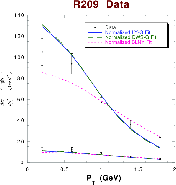
Figure 1: Comparison to the R209 data for the process $p+p\rightarrow\mu^{+}\mu^{-}+X$ process at $\sqrt{S}=62$ GeV. The data are the published experimental values. The curves are the results of the fits and are multiplied by the best-fit values of $1/N_{fit}$ given in Table III.

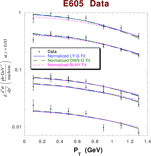
Figure 2: Comparison to the E605 data for the process $p+Cu\rightarrow\mu^{+}\mu^{-}+X$ at $\sqrt{S}=38.8$ GeV. The data are the published experimental values. The curves are the results of the fits multiplied by the best-fit values of $1/N_{fit}$ given in Table III.

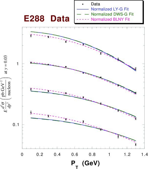
Figure 3: Comparison to the E288 data for the process $p+Cu\rightarrow\mu^{+}\mu^{-}+X$ at $\sqrt{S}=27.4$ GeV. The data are the published experimental values. The curves are the results of the fits and are multiplied by the best-fit values of $1/N_{fit}$ given in Table III.

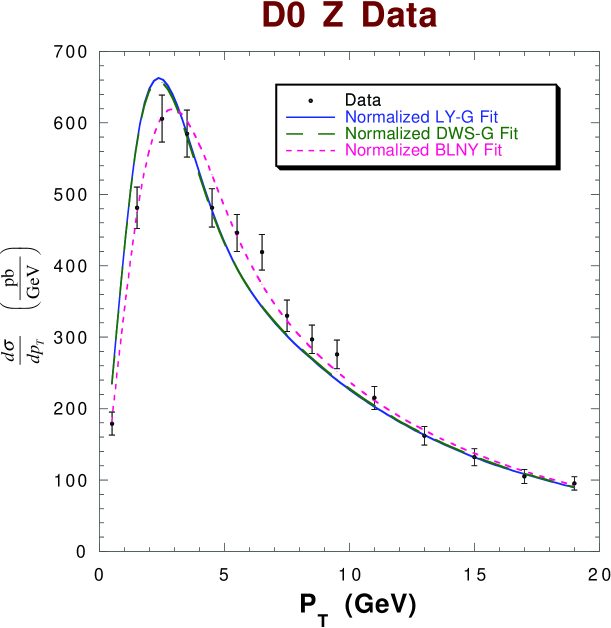
Figure 4: Comparison to the DØ -$Z$ Run-1 data. The data are the published experimental values. The curves are the results of the fits and are multiplied by the best-fit values of $1/N_{fit}$ given in Table III.

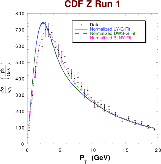
Figure 5: Comparison to the CDF-$Z$ Run-1 data. The data are the published experimental values. The curves are the results of the fits and are multiplied by the best-fit value of $1/N_{fit}$ given in Table III.

It is evident that the Gaussian BLNY parameterization fits the whole data sample noticeably better than the other two parameterizations, both in terms of $\chi^{2}$ per degree of freedom (dof) given in Table 3 and in terms of the pictorial comparison in Figs. 1-5. When compared to the Run-1 $Z$ data, the DWS-G and LY-G fits both fail to match the height and position of the peak in the transverse momentum distribution (Figs. 4 and 5). Similarly, according to Fig. 3, the BLNY parameterization leads to the best agreement with the E288 data. The three fits are indistinguishable when compared to the E605 data, cf. Fig. 2. Fig. 1 shows a clear difference between the BLNY fit and the other two fits for the lowest mass bin of the R209 data (the upper data in the Figure). However, the $\chi^{2}$ contribution from this mass bin is about the same for all three fits.

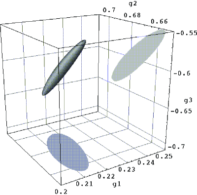
Figure 6: Uncertainty contour and two dimensional projections for the 3-parameter Gaussian BLNY form fit, cf. Eq. (12).

The error on the fitted nonperturbative parameters $g_{1}$, $g_{2}$ and $g_{3}$ can be calculated by examining the $\chi^{2}$ distribution of the fit. For the BLNY form

$$\widetilde{W}_{j\bar{k}}^{NP}(b,Q,Q_{0},x_{1},x_{2})={\textrm{exp}}\left[-g_{1}(1+g_{3}\ln{(100x_{1}x_{2})})-g_{2}\ln\left({\frac{Q}{2Q_{0}}}\right)\right]b^{2}$$ (13)

with $Q_{0}=1.6\mbox{\, GeV}$ and $b_{max}=0.5\mbox{\, GeV}^{-1}$, we found that

$$g_{1}=0.21_{-0.01}^{+0.01}\mbox{\, GeV}^{2}\;,\;g_{2}=0.68_{-0.02}^{+0.01}\mbox{\, GeV}^{2}\;,\;g_{3}=-0.6_{-0.04}^{+0.05}.$$ (14)

The errors in Eq. (14) were computed as follows. First, $\chi^{2}$ values were calculated around their minimum $\chi^{2}_{min}$ in order to obtain, in essence, a three dimensional function $\chi^{2}(g_{1},g_{2},g_{3})$. Next, we plotted an ellipsoid surface determined by the condition $\chi^{2}(g_{1},g_{2},g_{3})=\chi^{2}_{min}+1$ in the three-dimensional space of parameters $g_{i}$, cf. Fig. 6. The extremes in each coordinate for this surface were taken as the errors for the respective parameters. Finally, we note that using $\chi^{2}_{min}+1$ as the confidence limit for determining the values of $g_{i}$ in the presence of substantial systematic errors is generally idealistic, for the experiments often make judgments on systematic uncertainties that are not of a Gaussian nature. Further discussion of this issue can be found in the next Section.

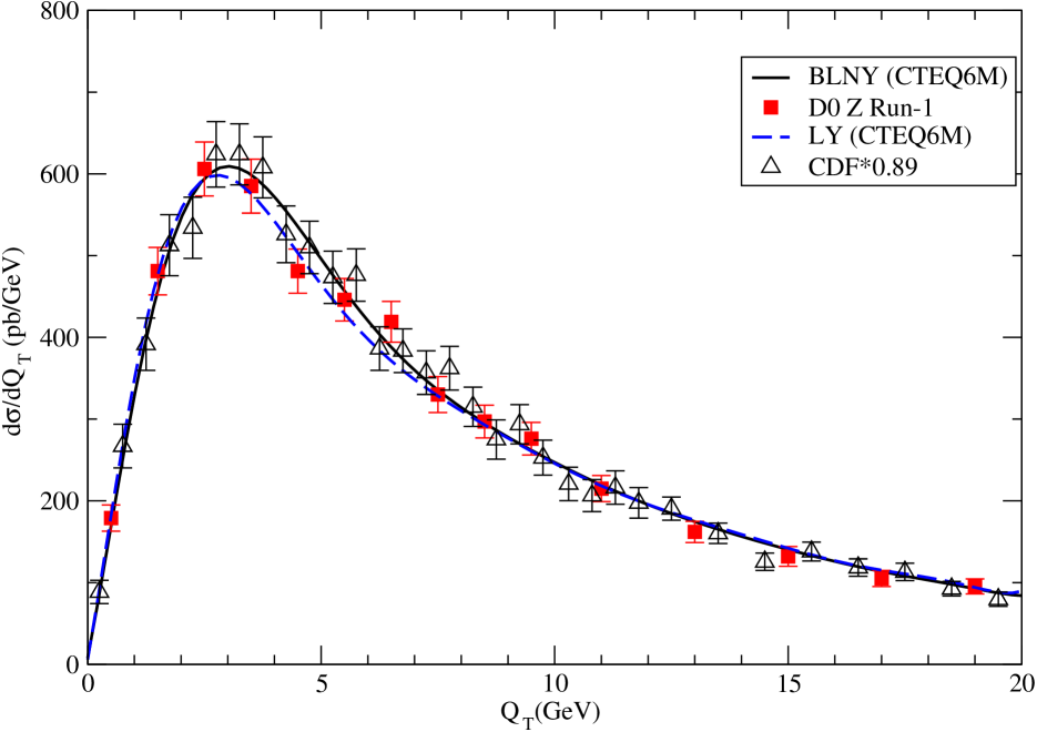
Figure 7: Transverse momentum distributions of $Z$ bosons at the Tevatron Run-1. The theory curves, calculated using the CTEQ6M PDF’s cteq6 and the BLNY parameterization (solid line) or the original LY parameterization, shown as dashed line, are compared to the DØ  data and CDF data. The data curves have been multiplied by an overall normalization factor 1.0 in DØ  data and 0.9 in CDF data.

IV Discussion

To fit the complete set of the experimental data (more than 100 data points), this analysis introduced 3 free parameters ($g_{1}$, $g_{2}$ and $g_{3}$) in the parameterization of $\widetilde{W}_{j\bar{k}}^{NP}$, together with the chosen values of the parameters $Q_{0}$ and $b_{max}$. In this paper and Ref. BLLY , we have chosen $Q_{0}=1.6$ GeV, which coincides with the lowest energy scale used in the CTEQ3M PDF set. This choice is nothing more than a matter of convenience, since it enforces positivity of the logarithm $\ln(Q/2Q_{0})$ in the $Q$ range of the fitted data ($Q\geq 5$ GeV). But $Q_{0}$ does not have to take that special value, since its variations can be compensated for in the full nonperturbative function $\widetilde{W}_{j\bar{k}}^{NP}$ by adjusting parameters $g_{1}$ and $g_{3}$ (at $g_{2}$ fixed). For instance, we could have chosen $Q_{0}$ to be equal to $1/b_{max}$ and rewrite Eq. (12) as

$$\widetilde{W}_{j\bar{k}}^{NP}(b,Q,Q_{0},x_{1},x_{2})={\textrm{exp}}\left[-g^{{}^{\prime}}_{1}(1+g^{{}^{\prime}}_{3}\ln{(100x_{1}x_{2})})-g^{{}^{\prime}}_{2}\ln(Qb_{max})\right]b^{2},$$ (15)

where $g^{{}^{\prime}}_{2}=g_{2}$, $g^{{}^{\prime}}_{1}=g_{1}-g_{2}\ln(2Q_{0}b_{max})$, and $g^{{}^{\prime}}_{3}=g_{3}g_{1}/g^{{}^{\prime}}_{1}$. This new form of $\widetilde{W}^{NP}_{j\bar{k}}$ would be completely identical to the original form in Eq. (12). Hence, the total number of parameters needed to describe $\widetilde{W}_{j{\bar{k}}}(b)$ in the used prescription is four, i.e., $g_{i}$ and $b_{max}$.

While the parameter $Q_{0}$ plays no dynamical role, the meaning of the parameter $b_{max}$ is quite different. Roughly speaking, its purpose is to separate nonperturbative effects from perturbative contributions through the introduction of the variable $b_{*}$ defined in Eq. (7). According to its definition, the variable $b_{*}$ is practically equal to $b$ when $b^{2}\ll b^{2}_{max}$. For $b\rightarrow\infty$, it asymptotically approaches $b_{max}$. Hence, in the factorized CSS representation (6) the perturbative part $\widetilde{W}^{pert}_{j{\bar{k}}}(b_{*})$ approaches its exact value (evaluated at $b$) when $b\rightarrow 0$, and it is frozen at $b_{*}\approx b_{max}$ when $b\rightarrow\infty$. While $b_{max}$ should lie in the perturbative region to make the computation of $\widetilde{W}^{pert}_{j\bar{k}}(b_{*})$ feasible, it is also desirable to make it as large as possible, to reduce deviations of $\widetilde{W}^{pert}_{j\bar{k}}$ from its exact behavior at smaller $b$. Note, however, that the changes in the behavior of $\widetilde{W}^{pert}_{j\bar{k}}$ due to the $b_{*}$ prescription, such as the loss of suppression of $\widetilde{W}^{pert}_{j\bar{k}}$ by the perturbative Sudakov factor at $b\gtrsim b_{max}$, can be compensated for by increasing the magnitude of the nonperturbative function $\widetilde{W}^{NP}_{j\bar{k}}$. Hence, in the $b_{*}$ prescription the nonperturbative function $\widetilde{W}^{NP}_{j\bar{k}}$ generally serves a dual purpose of the parameterization for truly nonperturbative effects and compensation factor for modifications in $\widetilde{W}^{pert}_{j\bar{k}}$ due to the $b_{*}$ variable. Consequently, the best-fit parameterization of $\widetilde{W}^{NP}_{j\bar{k}}$ depends on the choice of $b_{max}$.

Based on the fact that the $b_{*}$ prescription with the BLNY form of the non-perturbative function provides an excellent fit to the whole set of Drell-Yan-like data, we conclude that the $b_{*}$ prescription remains an adequate method for studies of resummed $Q_{T}$ distributions.This, however, does not mean that future tests and improvements of this method will not be necessary. For instance, one might consider a larger value of $b_{max}$ for the fit. Up to now, all the fits performed in the literature have taken $b_{max}$ to be $0.5{\,\mbox{GeV}}^{-1}$. However, $b_{max}$ could be chosen to be as large as $b_{0}/\mu_{F}^{0}$, where $b_{0}=2e^{-\gamma_{E}}\approx 1.122...$, and $\mu_{F}^{0}$ is the initial energy scale for the PDF set in use. Several of the most recent PDF sets, such as CTEQ6M cteq6 , MRST’2001 MRST2001 and MRST’2002 MRST2002 , use $\mu_{F}^{0}$ as low as 1 GeV. Correspondingly, for the new PDF sets $b_{max}$ can be as large as $1.122\mbox{\, GeV}^{-1}$. It will be interesting to test the $b_{*}$ prescription with such increased value of $b_{max}$ in a future study. Moreover, an approach alternative to the $b_{*}$ prescription was recently proposed in Refs. qiu1 ; qiu2 . Fig. 7 of Ref. qiu2 shows the comparison of this new theory calculation to the Run-1 CDF data, which should be compared to Fig. 5 of this paper. Furthermore, in Refs. joint ; joint2 , another method for performing the extrapolation to the large-$b$ region was proposed. To see the difference between the theory predictions for the Tevatron $Z$ data, one can compare Figs. 5 and 6 of Ref. joint2 to Figs. 5 and 4 of this paper. In a forthcoming publication BalazsNadolskyYuan2002 , we shall present a detailed comparison of various methods for description of large-$b$ physics to the Tevatron $Z$ data.

We would like to conclude this section with a remark about the dependence of our results on the choice of parton distribution functions. As noted above, the fitted nonperturbative function $\widetilde{W}_{j{\bar{k}}}^{NP}(b)$ in the CSS resummation formalism is correlated to the PDF’s used in the theory calculation. In the current fit, we have chosen to use CTEQ3M PDF’s to facilitate the comparison with the previous results in Ref. BLLY . The usage of a more modern PDF set with the BLNY parameterization of $\widetilde{W}^{NP}_{j\bar{k}}$ would result in a difference of a few percent in $Q_{T}$ distributions. Currently, such differences are of order of normalization errors quoted by the experiments. Hence, good agreement between the theory and data can be obtained by small normalization shifts in the data. We illustrate this point in Fig. 7, which compares the Tevatron Run-1 $Z$ data to the CSS resummation calculation performed using CTEQ6M PDF’s cteq6 and BLNY parameterization (12) with the best-fit nonperturbative parameters (14). By adjusting the normalization of the CDF data by the best-best value $N_{fit}=0.89$ in Fig. 7, the theory is brought in a good agreement with both sets of the Run-1 $Z$ data. For comparison, we also show in Fig. 7 the prediction from using CTEQ6M PDF’s and the original LY parametrization LY .

As the quality of the data improves in the future, the correlation between the nonpertubative function $\widetilde{W}_{j{\bar{k}}}^{NP}(b)$ and PDF’s will become more important. Hence, it will be certainly desirable to repeat the work done in this paper using the most recent set of PDF’s and potentially perform the joint global analysis of the PDF’s and CSS nonperturbative function. Furthermore, as the statistical errors decrease, correct treatment of the systematic errors (which are hardly of a Gaussian nature in many experiments) becomes ever more necessary. Therefore, a method more elaborate than the simple criterion $\chi^{2}_{min}+1$ used in the current analysis will be needed to determine the true confidence limit for the nonperturbative function. Recently, new efficient methods were proposed to perform the error analysis on the nonperturbative parameters in the PDF’s in the presence of systematic errors pdferr ; cteq6 ; MRST2002 . In the future, the same methods can also be applied to determine the errors for the nonperturbative parameters $g_{1}$, $g_{2}$, and $g_{3}$ in the BLNY nonperturbative function.

V Conclusions

We have shown for the first time that the complete set of low energy Drell-Yan data (R209, E605 and E288) and the Tevatron Run-1 $Z$-boson data can be simultaneously described by the CSS resummation formalism. This is the first truly global fit, which treats all the low energy Drell-Yan data and the Tevatron Z data on the same footing. This fact strongly supports the universality of the CSS nonperturbative function $\widetilde{W}_{j\bar{k}}^{NP}$. Just as the universality of the PDF’s allows us to predict the inclusive rate for a scattering process in hadron collisions, the universality of $\widetilde{W}_{j\bar{k}}^{NP}$ allows us to predict the transverse momentum distributions in production of single vector bosons and other similar processes at hadron colliders. For example, if true, the resummation formalism can be applied not only to the Drell-Yan pair production and $W$ (or $Z$) boson production, but also to associated production of Higgs and $W$ (or Higgs and $Z$) bosons hw , diphoton production twoW1 , $ZZ$ (or $WW$) pair production twoW2 , and $s$-channel neutral or charged Higgs boson production (induced from quark fusion with large Yukawa coupling to Higgs boson) qqhp . When these processes are measured to a good accuracy, they can be used to further test the CSS resummation formalism. Just as the PDF’s must be constantly refined in order to fit new experimental data, the nonperturbative function $\widetilde{W}_{j\bar{k}}^{NP}$ may also require modification in the future. At the current stage, the existing data shows remarkable preference for a Gaussian form of the nonperturbative function with $Q$ dependence predicted by the CSS formalism.

References

- (1) J. C. Collins, D. Soper, and G. Sterman, Nucl. Phys. B250 (1985) 199.
- (2) P.B. Arnold and R.P. Kauffman, Nucl. Phys. B349 (1991) 381.
- (3) C. Balázs and J.-W. Qiu, C.–P. Yuan, Phys. Lett. B355 (1995) 548.
- (4) C. Balázs and C.–P. Yuan, Phys. Rev. D56 (1997) 5558.
- (5) R.K. Ellis, D.A. Ross, and S. Veseli, Nucl. Phys. B503 (1997) 309.
-
(6)
C. Balázs, E.L. Berger, S. Mrenna, and C.–P. Yuan, Phys. Rev. D57
(1998) 6934;
C. Balázs, P. Nadolsky, C. Schmidt, and C.–P. Yuan, Phys. Lett. B489 (2000) 157. - (7) C. Balázs and C.–P. Yuan, Phys. Rev. D59 (1999) 114007.
-
(8)
S. Catani, E.D’Emilio, and L. Trentadue, Phys. Lett. B211 (1988)
335;
I. Hinchliffe and S.F. Novaes, Phys. Rev. D38 (1988) 3475;
R.P. Kauffman, Phys. Rev. D44 (1991) 1415;
C.–P. Yuan, Phys. Lett. B283 (1992) 395. - (9) C. Davies, B. Webber, and W. Stirling, Nucl. Phys. B256 (1985) 413.
- (10) G.A. Ladinsky and C.–P. Yuan, Phys. Rev. D50 (1994) 4239.
- (11) F. Landry, R. Brock, G. Ladinsky, and C.–P. Yuan, Phys. Rev. D63 (2001) 013004.
- (12) J.-W. Qiu and X.-F. Zhang, Phys. Rev. Lett. 86 (2001) 2724.
- (13) J.-W. Qiu and X.-F. Zhang, Phys. Rev. D63 (2001) 114011.
-
(14)
J. Paradiso, Ph.D. Thesis, Massachusetts Institute of Technology (1981);
D. Antreasyan, et al., Phys. Rev. Lett. 47 (1981) 12. - (15) G. Moreno, et al., Phys. Rev. D43 (1991) 2815.
- (16) A.S. Ito, et al., Phys. Rev. D23 (1981) 604.
-
(17)
F. Abe, et al., Phys. Rev. Lett. 67 (1991) 2937;
J.S.T. Ng, Ph.D. Thesis (1991), Harvard University preprint HUHEPL-12. - (18) DØ Collaboration (B. Abbott et al.), Phys. Rev. D61 (2000) 032004.
- (19) CDF Collaboration (T. Affolder et al.), Phys. Rev. Lett. 84 (2000) 845.
- (20) J. C. Collins and D. E. Soper, Nucl. Phys. B193, 381 (1981) [Erratum-ibid. B213, 545 (1983)]; Nucl. Phys. B197, 446 (1982).
- (21) G.P. Korchemsky and G. Sterman, Nucl. Phys. B437 (1995) 415.
- (22) H. L. Lai et al., Phys. Rev. D51 (1995) 4763.
- (23) P.L. McGaughey, et al., Phys. Rev. D50 (1994) 3038.
- (24) W.-K. Tung, private communication.
- (25) C. Balázs and C.–P. Yuan, Phys. Lett. B478, 192 (2000).
- (26) S. Mrenna and C.–P. Yuan, Phys. Lett. B416 (1998) 200.
- (27) C. Balázs, H.J. He, and C.–P. Yuan, Phys. Rev. D60 (1999) 114001
- (28) W. L. Anderson, ACM Trans. Math. Softw. 8, No. 4, p. 344 (1982).
- (29) C. Balázs, P. M. Nadolsky, C.–P. Yuan, in preparation.
- (30) E. Laenen, G. Sterman and W. Vogelsang, Phys. Rev. Lett. 84, 4296 (2000).
- (31) A. Kulesza, G. Sterman and W. Vogelsang, Phys. Rev. D 66, 014011 (2002).
- (32) J. Pumplin, D. R. Stump, J. Huston, H.-L. Lai, P. Nadolsky, and W.-K. Tung, JHEP 0207, 012 (2002).
- (33) A. D. Martin, R. G. Roberts, W. J. Stirling, and R. S. Thorne, Eur. Phys. J. C23, 73 (2002).
- (34) A. D. Martin, R. G. Roberts, W. J. Stirling and R. S. Thorne, arXiv:hep-ph/0211080.
-
(35)
W. T. Giele and S. Keller, Phys. Rev. D58, 094023 (1998);
W. T. Giele, S. A. Keller, and D. A. Kosower, arXiv:hep-ph/0104052;
M. Botje, Eur. Phys. J. C14, 285 (2000);
V. Barone, C. Pascaud and F. Zomer, Eur. Phys. J. C12, 243 (2000);
J. Pumplin, D. R. Stump, and W. K. Tung, Phys. Rev. D 65 (2002) 014011;
D. R. Stump et al., Phys. Rev. D 65 (2002) 014012;
J. Pumplin et al., Phys. Rev. D 65 (2002) 014013;
S. I. Alekhin, Phys. Rev. D63, 094022 (2001);
C. Adloff et al. [H1 Collaboration], Eur. Phys. J. C21, 33 (2001);
A. M. Cooper-Sarkar, J. Phys. G28, 2669 (2002). -
(36)
F. J. Landry, Ph. D. Thesis, Michigan State University, (2001);
also available as UMI-30-09135-mc (microfiche).