Solar Neutrinos Before and After KamLAND

Abstract:

We use the recently reported KamLAND measurements on oscillations of reactor anti-neutrinos, together with the data of previously reported solar neutrino experiments, to show that: (1) the total ⁸B neutrino flux emitted by the Sun is $1.00(1\pm 0.06)$ (1$\sigma$) of the standard solar model (BP00) predicted flux, (2) the KamLAND measurements reduce the area of the globally allowed oscillation regions that must be explored in model fitting by six orders of magnitude in the $\Delta m^{2}-\tan^{2}\theta$ plane, (3) LMA is now the unique oscillation solution to a CL of $4.7\sigma$, (4) maximal mixing is disfavored at $3.1\sigma$, (5) active-sterile admixtures are constrained to $\sin^{2}\eta\leq 0.13$ at $1\sigma$, (6) the observed ⁸B flux that is in the form of sterile neutrinos is $0.00^{+0.09}_{-0.00}$ (1$\sigma$), of the standard solar model (BP00) predicted flux, and (7) non-standard solar models that were invented to avoid completely solar neutrino oscillations are excluded by KamLAND plus solar data at $7.9\sigma$. We also refine quantitative predictions for future ⁷Be and $p-p$ solar neutrino experiments.

1 Introduction

KamLAND is the first experiment to explore with a terrestrial beam the region of neutrino oscillation parameters that is relevant for solar neutrino oscillations. This spectacular achievement [1] makes possible new studies of the physics of neutrinos  [2, 3, 4, 5, 6, 7, 8, 9, 10] and of the solar interior [11]. We concentrate here on refining the allowed regions in neutrino oscillation space and on what can be learned about the total ⁸B solar neutrino flux, as well as the sterile neutrino component of the ⁸B neutrino flux. The procedures we use have been described in refs. [2, 12].

We assume throughout this paper that CPT is satisfied and that the anti-neutrino measurements by KamLAND apply directly to the neutrino section. In fact, the first KamLAND results already show that CPT is satisfied in the weak sector to a characteristic accuracy of about $10^{-20}$ GeV [4].

We begin in section 2 by determining the allowed oscillation regions using the recently released KamLAND data. Our principal results, which are in good agreement with the analysis of the KamLAND collaboration [1], are summarized in figure 1 and in table 3. We also show that the numerical values of the physical quantities that we calculate in this paper are insensitive to the details of the analysis of the KamLAND data (see discussion at the end of section 6).

We derive in section 3 a global solution for the neutrino oscillation parameters using, together with the KamLAND measurements, all the available solar neutrino data from the chlorine [13], gallium [14, 15, 16], Super-Kamiokande [17], and SNO [18, 19] experiments. The enormous reduction in the size of the allowed oscillation regions is evident from a comparison of the ‘Before’ and ‘After’ allowed regions, figure 3 and figure 4.

We determine in section 4 the total ⁸B solar neutrino flux, as well as the uncertainties in the flux that are implied by the existing experimental data. This flux can be compared directly with the flux predicted by the standard solar model.

Could there be a large but unobservable flux of ⁸B solar neutrinos that reaches Earth in the form of sterile (right-handed) neutrinos? Prior to the announcement of the KamLAND results [1], the answer to this question was a resounding “Yes”[2, 20]. At $3\sigma$, the sterile component of the ⁸B flux could be, prior to KamLAND, as large as 1.1 times the BP00 predicted flux, which amounts to 50% of the total flux for this extreme case. However, the KamLAND measurement allows us to place a strong upper limit on the flux of sterile ⁸B neutrinos. We determine in section 5 the best-estimate sterile ⁸B neutrino flux and the associated uncertainties in the sterile flux.

We summarize and discuss our main conclusions in section 6.

2 KamLAND only

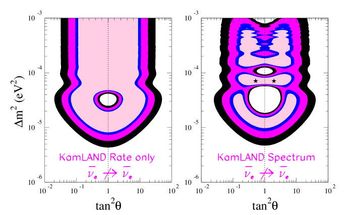
Figure 1: Anti-neutrino oscillation parameters regions allowed by KamLAND. The figure shows the allowed regions for anti-neutrino oscillation, $\bar{\nu}_{e}~{}\not\rightarrow~{}\bar{\nu}_{e}$, as implied by the first KamLAND results [1]. The contours shown in the left hand panel were calculated using only the total rate observed in the KamLAND experiment; the contours in the right hand panel were calculated using the measured KamLAND energy spectrum. The contours shown in figure 1 are $90$%, $95$%, $99$%, and $99.73$% ($3\sigma$)confidence limits. The dark crosses mark the best-fit values for the energy spectrum. The non-observation of anti-neutrino oscillations in the CHOOZ [21] reactor experiment rules out solutions with $\Delta m^{2}$ greater than $\sim 1\times 10^{-3}{\rm eV^{2}}$ at $3\sigma$ or $\sim 8\times 10^{-4}{\rm eV^{2}}$ at 99% CL .

Figure 1 shows the allowed regions for anti-neutrino oscillations that we have determined using the description of the detector operation and the measured data presented in the recent KamLAND publication [1]. The left hand panel of figure 1 shows the allowed regions calculated using only the KamLAND total event rate; the right hand panel shows the allowed regions calculated using the experimental energy spectrum, which also contains a rate normalization. In computing the right hand panel of figure 1, we also used the data from the CHOOZ reactor experiment. This experiment rules out solutions with $\Delta m^{2}$ greater than $\sim 1\times 10^{-3}{\rm eV^{2}}$ at $3\sigma$ or $\sim 8\times 10^{-4}{\rm eV^{2}}$ at 99% CL.

Section 2.1 contains our version (used in the following sections of the paper) of the science results from the KamLAND measurements and may be of general interest. Section 2.2 contains a description of how we do the data analysis and is rather specialized. We describe in sec. 2.3 Earth matter effects in the KamLAND experiment. The results of sec. 2.3 show that matter effects must be included in future precision analyses of the KamLAND experiment. We have carried out the KamLAND-only and the solar plus KamLAND analyses described in this paper both with and without including matter effects for the KamLAND experiment and have verified that, at the present level of accuracy for KamLAND measurements, the predictions for future experimental measurements are unaffected by including matter effects for KamLAND. Section 2.2 and Section 2.3 are rather technical and can be skipped by the reader who is primarily interested in the science.

We have verified that different plausible approaches to analyzing the KamLAND data do not lead to significant differences in the quantities in which we are most interested: the total ⁸B solar neutrino flux, the sterile component of the ⁸B neutrino flux, the CL at which maximal mixing is excluded, and the predictions for future solar neutrino experiments.

2.1 The KamLAND allowed regions

As expected, the allowed regions shown in figure 1 are in agreement with those reported by the KamLAND collaboration. It was necessary to establish explicitly this agreement in order to have confidence in the subsequent steps of our analysis, which involve determining: the globally allowed regions (section 3.1.1), predictions for future solar neutrino experiments (section 3.1.2), the total ⁸B solar neutrino flux (section 4), an upper limit to the sterile component of the ⁸B neutrino flux (section 5), and an upper limit to the CNO contribution of the solar luminosity (ref. [11]).

The results we obtain for the global solar plus KamLAND contours of the allowed regions, and all of the quantities derived from these contours, are essentially independent of the details of the analysis of the KamLAND results. We have verified this independence by analyzing the KamLAND measurements in a number of different ways (see discussion at the end of section 6).

The most important aspect of figure 1 is the demonstration by the KamLAND results that anti-neutrinos oscillate with parameters that are consistent with the LMA solar neutrino solution [22]. We shall exploit this extraordinary achievement in detail in the following sections. The symmetry shown in figure 1 with respect to the line $\theta=\pi/4$ (or $\tan^{2}\theta=1$) is just a reflection of the fact that the KamLAND experiment is an essentially vacuum experiment (but cf. sec. 2.3 and fig. 2) and hence the survival probabilities depend almost entirely upon $\sin^{2}2\theta$.

For the rates-only analysis, the best-fit oscillation parameters form a degenerate line in the $\Delta m^{2}$-$\tan^{2}\theta$ plane. For large $\Delta m^{2}$, the line only depends upon $\theta$ and is described by $\tan^{2}\theta=0.36$.

Expressed in terms of the rate expected if there were no flavor changes, the KamLAND rate is

$$R_{\rm KamLAND}~{}=0.611\pm 0.094\;.$$ (1)

The measured rate is in excellent agreement with the pre-KamLAND expectations [12]

$$R_{\rm KamLAND,\,expected}~{}=0.58^{+0.10}_{-0.27}\;,$$ (2)

based on purely solar neutrino experiments.

As can be seen in the right hand panel of figure 1 and as is summarized in table 1, the KamLAND spectral data lead to three local minima. The allowed region is separated into ‘islands.’ These islands correspond to oscillations with wavelengths that are approximately tuned to the average distance between the reactors and the detector, $180$ km. The best-fit point in the lowest mass island ($\Delta m^{2}=1.5\times 10^{-5}\,{\rm eV^{2}}$) is near the first-maximum in the oscillation probability (minimum in the event rate). The overall best-fit point ($\Delta m^{2}=7.1\times 10^{-5}\,{\rm eV^{2}}$) lies within the island around the second maximum in the oscillation probability. The tuning is less accurate for the best-fit point in the highest mass island.

For each of the allowed islands in neutrino oscillation parameter space that are shown in the right hand panel of figure 1 (analysis of the energy spectrum), table 1 gives the best-fit values of $\Delta m^{2}$ and $\tan^{2}\theta$. The global best-fit point for the KamLAND data set lies at $\Delta m^{2}=7.1\times 10^{-5}$ eV² and mixing angle $\tan^{2}\theta=0.52$. For the same mass difference, maximal mixing is slightly less favored, $\Delta\chi^{2}=0.4$. With the present statistical accuracy, KamLAND cannot discriminate between large angle (non-maximal) mixing and maximal mixing.

Table 1: KamLAND allowed regions. The table presents the best-fit oscillation parameters for the current 3$\sigma$-allowed LMA islands determined by the KamLAND energy spectrum (see figure 1). We also give the $\chi^{2}$ difference between the local minimum in each region and the global minimum.

$\Delta\bar{m}^{2}$	$\tan^{2}\bar{\theta}$	$\Delta\chi^{2}_{min}$
$7.1\times 10^{-5}$	$5.2\times 10^{-1}$ ($1.9\times 10^{0})$	0.0
$1.7\times 10^{-4}$	$3.5\times 10^{-1}$ ($2.8\times 10^{0})$	1.6
$1.5\times 10^{-5}$	$3.7\times 10^{-1}$ ($2.7\times 10^{0})$	3.0

At what level are other, non-LMA oscillation solutions excluded? For $\Delta m^{2}<10^{-6}{\rm eV^{2}}$, there is no significant oscillation probability in the KamLAND experiment. All such low $\Delta m^{2}$ solutions (like the previously-discussed LOW and Vacuum solar neutrino oscillation solutions), have $\Delta\chi^{2}>15.9$ and are excluded by at least $3.6\sigma$ (2 dof).

Comparing the total number of observed and expected events in KamLAND we find that alternative explanations to the solar neutrino problem that predict no deficit in the KamLAND experiment are now excluded at 3.6$\sigma$. This applies, for instance, to spin flavor precession, or flavor changing neutrino interactions which are now ruled out at 3.6$\sigma$ as the dominant mechanism for solar neutrino flavor conversion. In particular, all ‘non-standard solar model’ explanations of the ‘solar neutrino problem’ which assume particle physics with $P_{ee}=1$ (no neutrino oscillations) are also excluded by the KamLAND experiment at $3.6\sigma$.

2.2 KamLAND analysis

¿From the experimental point of view, KamLAND involves different systematic uncertainties than solar neutrino experiments. From a theoretical point of view, KamLAND uses anti-neutrinos to perform a pure disappearance experiment in vacuum. Solar neutrino studies use neutrinos to perform disappearance (or appearance) experiments in matter (or in vacuum). The analysis of the KamLAND data requires a treatment that is different from, and in many ways more simple than, the global analysis of solar neutrino data.

Using the data provided in the KamLAND paper [1], we calculate the positron spectrum in KamLAND detector with the procedures described in refs. [2, 23, 24, 25, 26]. In the absence of neutrino oscillations, we find (in agreement with ref. [1]) 86.8 expected neutrino events above 2.6 MeV visible energy, for 145.1 days of live time, a 408 ton fiducial mass with 3.46 $\times 10^{31}$ free target protons, detection efficiency of 78.3%, energy resolution $\sigma(E)/E=7.5\%/\sqrt{E}$, integrated total thermal power flux during the measurement live time of 254 Joule/${\rm cm^{2}}$, and relative fission yields from different fuel components as specified in ref. [1]. The positron energy spectrum that we calculate is in excellent agreement with the energy spectrum without oscillations presented by the KamLAND collaboration.

We perform, following the KamLAND collaboration, two analyses of the first KamLAND results: 1) including only the total event rate, and 2) including the total measured energy spectrum. For the rate only analysis, the $\chi^{2}$ can be written as  [1],

$$\chi^{2}_{\rm Rate}=\frac{(0.611-R(\theta,\Delta m^{2}))^{2}}{\sigma_{\rm R}^{2}}\;,$$ (3)

with $\sigma_{\rm R}^{2}~{}=~{}(0.085)^{2}~{}+~{}(0.041)^{2}$ and

$$R=1-\sin^{2}2\theta\langle\sin^{2}\left(\frac{\Delta m^{2}L}{4E_{\nu}}\right)\rangle\;.$$ (4)

We denote by $\langle\rangle$ the convolution over the energy spectrum, the interaction cross section, and the energy resolution function. For simplicity in the notation, we have neglected in writing eq. 4 all matter effects (see sec. 2.3 for details of the matter effects).

In the left hand panel of figure 1, we show the allowed regions (2 dof) that are obtained from this rate-only analysis. The vertical asymptotes can be calculated simply from eq. (3) since for large $\Delta m^{2}$ the quantity $\left<\sin^{2}\left(\Delta m^{2}L/4E_{\nu}\right)\right>$ averages to 0.5 . Thus in the large $\Delta m^{2}$ limit, the mixing angle boundary of the allowed region satisfies $\sin^{2}(2\theta)=-2\sigma_{\rm R}\sqrt{\Delta\chi^{2}_{CL}}~{}+~{}0.778$. Here $\Delta\chi^{2}$ is fixed by the CL of interest; $\Delta\chi^{2}=5.99(11.83)$ for 95% CL (for $3\sigma$ CL).

We included the data from the KamLAND energy spectrum in a way that has become conventional when analyzing low statistics binned data  [27], assuming that data is Poisson distributed. We define the $\chi^{2}$ function as

$$\chi^{2}(\Delta m^{2},\theta)=-2{\cal L}=$$ (5)

$${\rm min}_{\alpha}\sum_{i}\left[2(\alpha N_{i}^{\rm th}(\Delta m^{2},\theta)-N_{i}^{\rm exp})+2N_{i}^{\rm exp}\ln\left(\frac{N_{i}^{\rm exp}}{\alpha N_{i}^{\rm th}(\Delta m^{2},\theta)}\right)\right]+\frac{(\alpha-1)^{2}}{\sigma_{\rm sys}^{2}}\;,\ \ \ \ \ \ \ \$$

where $\alpha$ is an absolute normalization constant and $\sigma_{\rm sys}=6.42\%$ represents the systematic uncertainties presented in table 2 of ref. [1]. The KamLAND collaboration analyzed the event sample by separating the total rate from the spectrum shape and using a maximum likelihood method.

In the right hand panel of figure 1, we show the allowed regions (2 dof) that we obtain from our analysis of the KamLAND spectrum.

We have performed a series of tests of the dependence of the allowed solutions on the statistical treatment of the data. For example, we have performed a standard $\chi^{2}$ analysis using the first 5 energy bins above 2.6 MeV visible energy as presented by the KamLAND collaboration, but with all the events above the fifth bin ($E>4.725$ MeV) collected into a single bin (or into two bins). We then assumed Gaussian statistics for all bins. We find that the exact size and shape of the $3\sigma$ allowed regions of the KamLAND-only analysis depend mildly on the strategy adopted, i.e., whether we use eq. (5) or the standard $\chi^{2}$. However, the differences are unimportant for quantities calculated using the global solar plus KamLAND allowed regions. We have also studied the effect of carefully treating the energy dependence of the energy threshold error by computing, as a function of the oscillation parameters, the systematic uncertainty for each bin due to the estimated systematic error for the energy scale (1.91% at 2.6 MeV[1]). This refinement has no discernible effect on any of the quantities we calculate in this paper.

We discuss at the end of section 6 the small quantitative dependence upon analysis strategy of each of the quantities we calculate in this paper.

2.3 Matter effects in the KamLAND experiment

It is conventional to ignore matter effects in analyzing the KamLAND results. However, as we shall see below, matter effects can influence the calculated anti-neutrino event rate by as much as $4$% if the mass and mixing angle are near the region of maximum sensitivity. Thus matter effects will have to be included in future analyses of the KamLAND results when greater statistical and systematic precision are obtained.

In the results described in this paper, we have included matter effects by assuming that the anti-neutrinos traverse a constant density medium ($\rho=2.7\,{\rm gm\,cm^{-3}}$, cf. ref. [23])with the path length appropriate to each reactor. Since matter effects are small, the assumption of a constant density is an excellent approximation. Once matter effects are included, the survival probability for the KamLAND experiment also depends on the active-sterile admixture. However, allowing sterile neutrinos reduces the influence of matter effects with respect to what is calculated for the pure active case.

To the accuracy that can be discerned by even the most expert eye, matter effects do not change the contours of figures given in the present paper.

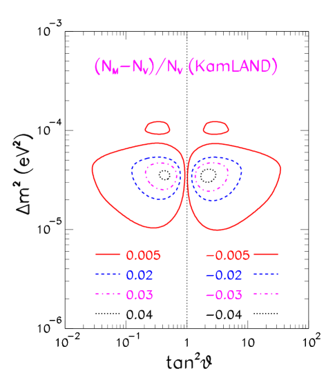
Figure 2: Matter effects in the KamLAND reactor experiment. The contours depict the fractional difference, defined in eq. 6, in the event rate calculated with and without including matter effects from anti-neutrinos traversing the Earth.

We define, $F({\rm matter~{}vs~{}vacuum})$, as the fractional difference in the event rate for the KamLAND detector calculated with and without including matter effects in the Earth. Thus

$$F({\rm matter~{}vs~{}vacuum})~{}=~{}\frac{R_{\rm matter}-R_{\rm vacuum}}{R_{\rm vacuum}}\,.$$ (6)

Figure 2 shows the contours of $F({\rm matter~{}vs~{}vacuum})$ in the $\Delta m^{2}$-$\tan^{2}\theta$ plane for active neutrinos. The maximum value of $|F({\rm matter~{}vs~{}vacuum})|$ corresponds to -4.2% (+4.3%) at $\Delta m^{2}~{}=~{}3.55\times 10^{-5}{\rm~{}eV^{2}}$ and $\tan^{2}\theta=0.43(2.18)$. Within the $1\sigma(3\sigma)$ allowed region of the analysis of the KamLAND energy spectrum (cf. the right hand panel of fig. 1), the maximum value of $|F({\rm matter~{}vs~{}vacuum})|$ corresponds to $0.9$% ($3.9$%). The maximum change in $\chi^{2}$ due to including matter effects in the KamLAND-only analysis is 0.2 (1.5) at $1\sigma(3\sigma)$. At the best-fit point for the analysis of the KamLAND energy spectrum, matter effects change the value of $\chi^{2}$ by only 0.1%.

We anticipate the results given latter in sec. 3 (see especially fig. 4) by noting that the matter effects in the KamLAND experiment are somewhat less important within the globally allowed solar plus KamLAND oscillation regions. For the global solution, $|F({\rm matter~{}vs~{}vacuum})|$ varies between $0.9$% ($2.7$%) at $1\sigma(3\sigma)$. The maximum change in $\chi^{2}$ in the global analysis due to matter effects is 0.2 (1.0).

For simplicity, we have described in the rest of this paper the KamLAND experiment as if matter effects could be completely ignored.

3 Global solutions: solar plus KamLAND

We present and discuss in section 3.1 the allowed regions in neutrino oscillation parameter space that are permitted at $3\sigma$ by the combined solar and KamLAND experimental data (see especially figure 4). We also present in this section (see especially table 2) the predictions of future solar neutrino observables that are calculated using the current global oscillation solutions.

In order to isolate the crucial measurements that have identified LMA as the correct description of solar neutrino oscillations, we present in section 3.2 the results of an analysis of just the rates of the solar neutrino experiments. We show in this section that, if we did not have the essentially undistorted electron recoil energy spectrum measured by Super-Kamiokande and confirmed by SNO, vacuum oscillations would be the preferred solution prior to the KamLAND measurements.

We include two sections that are primarily intended for aficionados of neutrino oscillation analyses. We outline briefly in section 3.3 how we have combined the solar and the KamLAND analyses. We have already described in section 2.2 how we have analyzed the KamLAND measurements. In section 3.3.1, we summarize our treatment of the solar data. We describe in section 3.3.2 our treatment of the sterile component of the solar neutrino flux.

3.1 Scientific results

We describe in section 3.1.1 the allowed regions in neutrino oscillation space that are determined by the solar and KamLAND data and in section 3.1.2 we present predictions for future solar neutrino experiments of the presently allowed global oscillation solutions.

3.1.1 Allowed regions

Figure 3 presents the ‘Before’ figure, the allowed neutrino oscillation regions for all the available solar neutrino data prior to the announcement of the first KamLAND results. We show in figure 3 the results of our analysis for this paper of the pre-KamLAND solar neutrino data. We include here for the first time the recently reported GNO measurements [16]; this inclusion does not affect figure 3 significantly. Our calculational procedures, which are described in ref. [12], contain some refinements not taken account of in other analyses. However, the overall results for the pre-KamLAND allowed regions are very similar in most treatments, cf. [28].

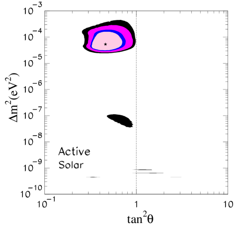
Figure 3: Before: Solar neutrino oscillations before KamLAND. The contours shown in figure 3 are $90$%, $95$%, $99$%, and $99.73$% ($3\sigma$)confidence limits. The global best-fit points are marked by a star.The input data used in constructing the figure include all the available solar neutrino measurements [13, 18, 19, 14, 15, 16, 17] and the neutrino fluxes and uncertainties predicted by the BP00 solar model [29] for all but the ⁸B flux. The ⁸B neutrino flux is treated as a free parameter.

Figure 4 displays the ‘After’ figure, the much reduced allowed regions that are determined by including the recently announced KamLAND measurements[1] together with the solar neutrino data.

Figure 4: After: Solar neutrino oscillations after KamLAND. The allowed contours shown in figure 3 include the recent KamLAND measurements and all the available solar neutrino data [13, 14, 15, 16, 17, 18, 19]. The contour limits are the same as in figure 1 and figure 3.

Comparing figure 3 with figure 4, we see that KamLAND has shrunk enormously the allowed parameter space that is accessible to theoretical models, by five orders of magnitude in $\Delta m^{2}$ and one order of magnitude in $\tan^{2}\theta$. The LMA region in parameter space is the only remaining allowed solution. The best-fit LOW solution is excluded at $4.8\sigma$ and vacuum solutions are excluded at $4.9\sigma$. The once ‘favored’ SMA solution is now excluded at $6.1\sigma$.

The allowed range for the mixing angle within the 1$\sigma$ (3$\sigma$) region shown in the ‘After’ figure 4 is

$$0.36(\,0.27)<\tan^{2}\theta<0.58\,(0.94)\,.$$ (7)

For the pre-KamLAND analysis, figure 3, the allowed $3\sigma$ domain for the mixing angle was $0.26<\tan^{2}\theta<0.98$. Therefore, the allowed range of mixing angles has only been marginally improved by the inclusion of the KamLAND data.

At what confidence level is maximal mixing excluded? There are no solutions with $\tan^{2}\theta=1$ at the $3.1\sigma$ CL. For the pre-KamLAND analysis, figure 3, there were no solutions with maximal mixing within the LMA region at $3.1\sigma$. However, maximal mixing was still allowed at $2.8\sigma$ within the vacuum solution regions, which is now excluded.

Figure 5 shows how solar neutrino experiments break the symmetry of the survival probability, $P_{\rm ee}\left(E\right)$, about a mixing angle of $\theta=\pi/2$ that exists for vacuum oscillation experiments. Vacuum oscillation survival probabilities are identical for two mixing angles $\theta_{1}$ and $\theta_{2}$, with $\theta_{2}=\pi/2~{}-~{}\theta_{1}$ and a fixed value for $\Delta m^{2}$. The left hand panel shows the vacuum survival probabilities for a source-detector separation of 180 km, similar to the actual experimental situation for KamLAND. The right hand panels displays the daytime survival probabilities for the two LMA solar neutrino oscillation solutions. Matter effects in the Sun are responsible for the different LMA survival probabilities.

Which solar neutrino experiments choose the lower probabilities (the smaller value for $\tan^{2}\theta$)? Originally, the chlorine experiment, in conjunction with the standard solar model predictions, indicated strongly that the smaller probabilities were correct. The measured event rate in the chlorine experiment, $\sim 2.6$ SNU [13], was closer to $0.35$ of the standard solar model prediction than to $0.65$ of the solar model prediction ($\sim 8$ SNU) [29]. This result was confirmed by the comparison of the Super-Kamiokande $\nu-e$ scattering measurements with the SNO CC measurement [30]. The comparison within the same experiment of the SNO CC and NC rates selects unambiguously the curve with the lower survival probabilities [18].

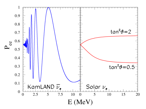
Figure 5: Breaking the degeneracy: $P_{\rm ee}$ vs $E$. Figure 5 shows the survival probability, $P_{\rm ee}$, as a function of neutrino energy, $E$, for two mixing angles related by $\theta_{2}=\pi/2~{}-~{}\theta_{1}$ ($\theta_{1}=35.3^{0},\tan^{2}\theta_{1}=0.5,\tan^{2}\theta_{2}=2.0$), with $\Delta m^{2}=7\times 10^{-5}{\rm~{}eV^{2}}$. The left hand panel shows the survival probability (averaged over $0.1$ MeV energy bins) in vacuum for a source-detector separation of $180$ km. The vacuum survival probabilities are identical for $\theta_{1}$ and $\theta_{2}$. The right hand panel shows the daytime LMA oscillation solutions for solar neutrinos. Matter effects in the Sun cause the differences between the two solar solutions.

Finally, we have evaluated the present status of ‘non-standard’ solar model explanations of the solar plus KamLAND data under the hypothesis of standard particle physics. We perform a fit to the total measured rates in the chlorine [13], gallium [14, 15, 16], Super-Kamiokande [17], SNO CC [18], and SNO NC [18] experiments, allowing the dominant $p-p$, ⁸B, ⁷B and CNO fluxes to vary freely but imposing the luminosity constraint (see [31] and references therein for details). We find that $\chi^{2}_{\rm min,solar}=53.9$ for $2$ dof (5 rates - 4 free fluxes + 1 constraint), which implies that non-standard solar model explanations of the solar data can be excluded at $7\sigma$. Adding to the analysis the evidence of antineutrino disappearance observed in the KamLAND experiment, we find that non-standard solar models invented to avoid solar neutrino oscillations are excluded by solar plus KamLAND experiments at $7.9\sigma$.

3.1.2 Predictions for future experiments

Table 2 presents the best-fit predictions and the expected ranges for some important solar neutrino observables. The results summarized in table 2 correspond to the globally allowed oscillation regions shown in figure 4. We consider predictions for SNO, for a large SK-like neutrino-electron scattering experiment, and for a neutrino-electron scattering detector, BOREXINO [32] or KamLAND [23], that observes the ⁷Be solar neutrinos. We also include predictions for a generic $p-p$ neutrino detector. The notation used here is the same as in ref. [12].

Table 2: Post-KamLAND Predictions. This table presents for future solar neutrino observables the best-fit predictions, and the $1\sigma$ and $3\sigma$ ranges, that were obtained from the global analysis shown in figure 4.

Observable	b.f. $\pm 1\sigma$	b.f $\pm 3\sigma$
AN-D (SNO CC) (%)	$3.3^{+0.7}_{-0.6}$	$3.3^{+5.7}_{-3.1}$
AN-D (SK ES) (%)	$1.9\pm 0.4$	$1.9^{+2.5}_{-1.8}$
$[$R (7Be)$]$ $\nu-e$ scattering	$0.64\pm 0.02$	$0.64^{+0.08}_{-0.04}$
AN-D (7Be) (%)	$0.0^{+0.0}_{-0.0}$	$0.0^{+0.1}_{-0.0}$
$[$R (8B)$]$ $\nu-e$ scattering
($T_{\rm th}=3.5$ MeV)	$0.46\pm 0.03$	$0.46\pm 0.04$
($T_{\rm th}=5$ MeV)	$0.45\pm 0.03$	$0.45\pm 0.04$
$[p$-$p]$ $\nu-e$ scattering
($T_{\rm th}=100$ keV)	$0.697\pm 0.023$	$0.697^{+0.064}_{-0.042}$
($T_{\rm th}=50$ keV)	$0.693\pm 0.024$	$0.693^{+0.064}_{-0.043}$

The day-night asymmetry $A_{\rm N-D}$ is defined in terms of the Day and the Night event rates by the expression

$$A_{\rm N-D}~{}=~{}2{\rm{[Night-Day]}\over{[Night+Day]}}~{}.$$ (8)

The prediction for the day-night asymmetry in the SNO CC measurement is one of the most interesting new results to come from the much smaller, post-KamLAND allowed regions (see discussion of earth matter effects in the LMA regime in refs. [33, 34, 35]).

Within the unique 1$\sigma$ region (2 dof), the prediction is

$$A_{\rm N-D}({\rm SNO~{}CC})~{}=~{}3.3^{+0.7}_{-0.6}\%\,.$$ (9)

Within the $3\sigma$ region (2 dof), $A_{\rm N-D}({\rm SNO~{}CC})~{}=~{}3.3^{+5.7}_{-3.1}\%\,.$

An accurate day-night asymmetry measurement in the SNO CC mode could, in principle, help to discriminate between larger and smaller values of $\Delta m^{2}$. For values of $\Delta m^{2}<10^{-4}{\rm eV^{2}}$ within the currently allowed $3\sigma$ (2 dof) region,

$$A_{\rm N-D}({\rm SNO~{}CC})~{}=~{}3.3^{+5.7}_{-1.6}\%\,,~{}(\Delta m^{2}<10^{-4}\,{eV^{2}})\,.$$ (10)

For values of $\Delta m^{2}\geq 10^{-4}{\rm eV^{2}}$, the day-night asymmetry is small,

$$A_{\rm N-D}({\rm SNO~{}CC})~{}=~{}0.6^{+1.1}_{-0.4}\%\,,~{}(\Delta m^{2}\geq 10^{-4}\,{eV^{2}})\,.$$ (11)

Unfortunately, it will be very difficult to reach the required experimental precision.

In table 2 we also present the predicted day-night asymmetry at a SK-like neutrino-electron scattering detector with a threshold $E_{\rm th}=5$ MeV. For ES the day-night effect is decreased relative to pure CC interactions by the contribution of the neutral currents.

The prediction for the reduced ⁷Be $\nu-e$ scattering rate,

$$[{\rm{}^{7}Be}]~{}\equiv~{}\frac{\rm Observed~{}\nu-e~{}scattering~{}rate}{\rm BP00~{}predicted~{}rate}~{},$$ (12)

is remarkably precise and remarkably stable. Within the $1\sigma$ allowed region, the pre-KamLAND prediction was $[{\rm{}^{7}Be}]~{}=0.64\pm 0.03,~{}1\sigma$ [12]. The post-KamLAND prediction for the currently allowed $1\sigma$ region is

$$\left[{\rm{}^{7}Be}\right]_{\rm post-KamLAND}~{}=0.64\pm 0.02\,.$$ (13)

The predicted event rate for the ⁷Be rate experiment has a precision of $\pm 3$% in units of the rate calculated with the BP00 flux and assuming no neutrino oscillations.

Now that LMA is the only oscillation solution allowed at $3\sigma$, the predicted ⁷Be day-night asymmetry averaged over a year is too small to be observed. Within the current 3$\sigma$ allowed oscillation region, the limit on the predicted values of $A_{\rm N-D}$ is

$$\left|A_{\rm N-D}({\rm{}^{7}Be})\right|~{}<~{}0.001.$$ (14)

We also include in table 2 predictions for the rate at which ⁸B neutrinos will be scattered by electrons resulting in recoil electrons in BOREXINO or KamLAND above two different electron recoil kinetic-energy energy thresholds, $T_{\rm th}=3.5$ MeV and $T_{\rm th}=5$ MeV. The predictions are given in terms of the reduced event rate for ⁸B neutrinos, [R(⁸B)], which is defined analogously to [⁷Be] [see eq. (12)] relative to the scattering rate predicted for the standard solar model flux with no oscillations. The predicted ranges of [R(⁸B)] are obtained from the allowed 1$\sigma$ or 3$\sigma$ regions in the three parameter space of $\Delta m^{2},\tan^{2}\theta$, and $f_{\rm B,total}$. Not surprisingly, the predicted ⁸B neutrino-electron scattering rates are essentially identical to the neutrino-electron scattering rates measured by the SNO [18] and Super-Kamiokande [17] experiments, which are $0.47\pm 0.05$ and $0.465\pm 0.015$, respectively. For plausible assumptions about how the BOREXINO detector will operate, one expects [12] $\sim 175$ events above a $3.5$ MeV recoil electron energy threshold and $\sim 110$ events per year above a $5$ MeV threshold.

In addition, we have evaluated the predictions for a generic $p-p$ neutrino-electron scattering detector. The reduced rate for this detector is defined by the relation

$$[p-p]~{}\equiv~{}\frac{\rm Observed~{}\nu-e~{}scattering~{}rate}{\rm BP00~{}predicted~{}rate}~{}.$$ (15)

We present the predicted rate for two plausible kinetic energy thresholds, $100$ keV and $50$ keV. The predicted rate is precise and robust. The precision of the prediction is $\pm 3$%; the best-fit predictions have changed by less than $1$% from the pre-KamLAND predictions [12].

The principal differences between the post-KamLAND predictions summarized in table 2 and the pre-KamLAND predictions given in table 2 of ref. [12] are a consequence of the disappearance of the LOW and the vacuum solutions. As a consequence, no significant day-night asymmetry nor seasonal variations are expected for ⁷Be neutrino measurements by BOREXINO or KamLAND. For all other observables, the main effect is the reduction of the 1$\sigma$ LMA ranges. Within the 3$\sigma$ LMA ranges, the changes are generally insignificant.

3.2 Rates only analysis

It is instructive to carry out a global analysis using only the total measured rates in the chlorine [13], gallium [14, 15, 16], Super-Kamiokande [17], SNO CC [18], and SNO NC [18] experiments. In this simplified analysis, we ignore all spectral energy data and all measurements of the zenith-angle (or day-night) dependence. We let the total ⁸B neutrino flux be a free variable in the standard rates-only analysis. For simplicity, we consider pure active, or pure sterile, neutrino oscillations. Therefore, the rates-only analysis has three degrees of freedom ($\Delta m^{2},\,\tan^{2}\theta$, and the ⁸B neutrino flux) and five measured rates.

The best-fit solution lies in the vacuum region. The oscillation parameters of the best fit solution are: ${\Delta m^{2}=8\times 10^{-11}{\rm\,eV^{2}},\,\tan^{2}\theta=0.30(3.35)}$ with $\chi^{2}_{\rm min}=2.2$. The values of $\chi^{2}_{\rm min}$ for the other well known solutions are: SMA (3.1) , LMA (3.8), and LOW (8.6), and pure sterile (23.1). All four solutions for active neutrinos, VAC, SMA, LMA, and LOW are allowed at $3\sigma$ in the rates-only analysis. If only rates are considered, the VAC, SMA, and LMA solutions are essentially equivalent.

We have done several tests to determine the robustness of this conclusion. The vacuum solutions always appear to be slightly preferred in the rates-only analyses, but the relative order of SMA-LMA can be reversed by slightly changes (such as using the original SNO CC data [30] with a 6.75 MeV threshold rather than the more recent data [18] with a 5.0 MeV threshold).

This analysis illustrates the fact that the measurement of the essentially undistorted recoil electron energy spectrum by Super-Kamiokande [17], which was confirmed by SNO [18], was required in order to establish, prior to the KamLAND measurements, that LMA was the favored solution. Previous rates-only analyses have established the critical importance of the Super-Kamiokande spectrum analysis [36, 37]. However, this is the first calculation that we know about in which all five of the currently available rate experiments have been included.

3.3 KamLAND plus Solar Analysis

It is convenient and conventional to discuss the experimentally determined ⁸B neutrino flux in units of the flux predicted by the standard solar model. Let $f_{\rm B,\,total}$ be the ratio of the total ⁸B solar neutrino flux to the flux predicted by the BP00 standard solar model, i.e.,

$$f_{\rm B,\,total}~{}\equiv~{}\frac{\phi(^{8}{\rm B})}{~{}\phi(^{8}{\rm B})_{\rm BP00}}\,,$$ (16)

where $\phi(^{8}{\rm B})_{\rm BP00}~{}\equiv~{}5.05\times 10^{6}\,{\rm cm^{-2}s^{-1}}$ [29].

We allow for the possibility that the ⁸B neutrino flux that arrives at Earth contains a significant component of sterile neutrinos which we parameterize in terms of the active-sterile admixture parameter $\sin^{2}\eta$ (See Sec. 3.3.2).

We calculate the global $\chi^{2}$ by fitting to all the available data, solar plus reactor. Formally, the global $\chi^{2}$ can be written in the form

$$\chi^{2}_{\rm global}~{}=~{}\chi^{2}_{\rm solar}(\Delta m^{2},\tan^{2}\theta,f_{\rm B,\,total},\sin^{2}\eta)~{}+~{}\chi^{2}_{\rm KamLAND}(\Delta m^{2},\tan^{2}\theta)\,.$$ (17)

There are four free parameters in $\chi^{2}_{\rm global}$, $\Delta m^{2},\tan^{2}\theta,f_{\rm B,\,total},$ and $sin^{2}\eta$, although $\chi^{2}_{\rm KamLAND}$ depends only on $\Delta m^{2},$ and $\tan^{2}\theta$. The most computationally intensive task in our analysis of solar plus KamLAND data, computing the multi-dimensional $\chi^{2}$ for all of the solar neutrino data, was calculated before the KamLAND announcement [1] and stored. This data set amounted to about 9.4 gigabytes. We do not include the CHOOZ data [21] explicitly in eq. 17 since the combined solar data also excluded larger values of $\Delta m^{2}$.

We have carried out a global analysis [12] of the combined solar neutrino data (80 measurements), see the discussion in section 3.3.1 below, and the KamLAND data (as described in section 2.2). We also consider the possibility that the ⁸B neutrino flux that arrives at Earth contains a significant component of sterile neutrinos. We describe in section 3.3.2 the aspects of the analysis that are related to sterile neutrinos.

3.3.1 Solar analysis

The details of our calculational methods are described in ref. [12]. We treat the ⁸B solar neutrino flux as a free parameter, but adopt the predictions of the BP00 solar model [29] for the other neutrino fluxes and uncertainties. The free ⁸B strategy adopted in the present paper was, in ref. [12], the preferred analysis procedure among the three analysis strategies that were used earlier.

We summarize briefly in this subsection the main features of our analysis of solar neutrino data.

For the solar neutrino analysis, we use 80 data points. We include the two measured radiochemical rates, from the chlorine [13] and the gallium [14, 15, 16] experiments, the 44 zenith-spectral energy bins of the electron neutrino scattering signal measured by the Super-Kamiokande collaboration  [17], and the 34 day-night spectral energy bins measured with the SNO [18, 19, 38] detector. The average rate for the gallium experiments [14, 15, 16] has been updated to $70.8\pm 4.4$ SNU by including the preliminary GNO data reported at Neutrino 2002 [16].

We take account of the BP00 [29] predicted fluxes and uncertainties for all solar neutrino sources except for ⁸B neutrinos. The Super-Kamiokande [17] and SNO [18, 19] experiments can now determine the ⁸B solar neutrino flux at a level of precision that is comparable with the precision of the BP00 prediction. Therefore, we treat the total ⁸B solar neutrino flux as a free parameter to be determined by experiment and to be compared with solar model predictions.

Following the SNO collaboration [19], we have considered together (consistent with the way they are measured) the SNO charged current, neutral current, and electron scattering events. For each point in neutrino oscillation parameter space, we have computed the 34 day-night spectrum energy bins by convolving the computed survival probabilities with the appropriate neutrino cross sections, as well as the experimental energy resolution and sensitivity functions.

We include the errors and their correlations for all of these observables. We construct an $80\times 80$ covariance matrix that includes the effect of correlations between the differ error as off diagonal elements. The errors and their correlations are described in in the Appendix of ref. [2] and in section 5.4 of ref. [12]

The analysis of the theoretical and experimental uncertainties is subtle. Many of the differences in the precise borders of the allowed oscillation regions that are reported by different groups may be traced to variations in the ways in which the errors are treated. We have performed the calculations accurately, although some of the refinements we have used are computationally demanding. As described in the Appendix of ref. [2], we include the energy dependencies and the correlations of the chlorine and gallium neutrino absorption cross sections. For both the Super-Kamiokande and the SNO experiments, we take account of the energy dependence and the correlation of the ⁸B spectral energy shape errors, the absolute energy scale errors, and the energy resolution errors.

3.3.2 Sterile component

We have also considered the possibility that $\nu_{e}$ oscillates into a state that is a linear combination of active ($\nu_{a}$) and sterile ($\nu_{s}$) neutrino states,

$$\nu_{e}\to\cos\eta\,\nu_{a}\,+\,\sin\eta\,\nu_{s}\,,$$ (18)

where $\eta$ is the parameter that describes the active-sterile admixture. This admixture arises in the framework of 4-$\nu$ mixing [39]. The total ⁸B neutrino flux can be written

$$\phi({\rm{}^{8}B})_{\rm total}~{}=~{}\phi(\nu_{e})~{}+~{}\phi(\nu_{a})~{}+~{}\phi(\nu_{s}),$$ (19)

where $\phi(\nu_{s})~{}=~{}\tan^{2}\eta\times\phi(\nu_{a})$.

The solar neutrino data analysis depends on four parameters: the oscillation parameters $\Delta m^{2}$ and $\tan^{2}\theta$, the total ⁸B neutrino flux $f_{\rm B,\,total}$ [see eq. (16)], and the sterile component characterized by $\sin^{2}\eta$. We can also characterize the sterile contribution to the total flux in terms of $f_{\rm B,\,sterile}$, which is defined as

$$f_{\rm B,\,sterile}~{}\equiv~{}\frac{~{}\phi(^{8}{\rm B,\,sterile})}{\phi(^{8}{\rm B})_{\rm BP00}}\,.$$ (20)

We obtain from eqs. (19) and (18) the relation

$$f_{\rm B,\,sterile}=f_{\rm B,\,total}\sin^{2}\eta\left(1-P_{ee}(E,\Delta m^{2},\tan^{2}\theta,\sin^{2}\eta)\right).$$ (21)

Thus for a given set of parameters $\Delta m^{2}$, $\tan^{2}\theta$, $f_{\rm B,\,total}$ and $\sin^{2}\eta$, the inferred sterile flux parameter $f_{\rm B,\,sterile}$ is an energy dependent, and time dependent, function. However, the energy and time dependences are mild since, for the LMA solution, $P_{ee}$ is nearly constant for the ⁸B neutrino energies that are accessible to direct measurement.

In this paper, we account for the mild energy and time dependences by defining $f_{\rm B,\,sterile}$ as the average sterile flux parameter inferred for the SNO experiment, i.e.,

$$f_{\rm B,\,sterile}=f_{\rm B,\,total}\sin^{2}\eta\left(1-\langle P_{ee}(E,\Delta m^{2},\tan^{2}\theta,\sin^{2}\eta)\rangle_{\rm SNO}\right)$$ (22)

where $\langle P_{ee}(E,\Delta m^{2},\tan^{2}\theta,\sin^{2}\eta)\rangle_{\rm SNO}$ is

$$\langle P_{ee}(\Delta m^{2},\tan^{2}\theta)\rangle_{\rm SNO}~{}=~{}\frac{\int\!dE_{\nu}\,\phi^{\rm SSM}({\rm{}^{8}B},\,E_{\nu})\sigma_{e}(E_{\nu})P_{ee}(E_{\nu},\Delta m^{2},\tan^{2}\theta)}{R^{\rm SSM}_{\rm SNO}}\,.$$ (23)

Here $P_{ee}$ is the average survival probability and $R^{\rm SSM}_{\rm SNO}$ is the predicted SSM [29] rate for the CC SNO measurement [18, 30] in the absence of neutrino oscillations,

$$R^{\rm SSM}_{\rm SNO}=\int\!dE_{\nu}\,\phi^{\rm SSM}({\rm{}^{8}B},\,E_{\nu})\sigma_{e}(E_{\nu}).$$ (24)

The cross section $\sigma_{e}(E_{\nu})$ [40, 41] is the weighted average cross-section for the CC reaction, $\nu_{e}+{{}^{2}H}~{}\rightarrow~{}e^{+}+n+p$, for the neutrino energy $E_{\nu}$ . The average includes the experimental energy resolution function, ${\rm Res}(T,\,T^{\prime})$, where $T(T^{\prime})$ is the measured (true) recoil kinetic energy of the electron. Thus

$$\sigma_{e}(E_{\nu})=\int_{T_{\rm min}}^{T_{\rm max}}\!dT\int_{0}^{{T_{\rm max}}^{\prime}(E_{\nu})}\!dT^{\prime}\,{\rm Res}(T,\,T^{\prime})\,\frac{d\sigma_{e}(E_{\nu},\,T^{\prime})}{dT^{\prime}}\ .$$ (25)

The lower limit, $T_{\rm min}$, in the integral in eq. (25) is taken here to be the threshold, 5 MeV, used by the SNO Collaboration in ref. [18]. The calculated value for the CC rate is not sensitive to the assumed value of $T_{\rm max}$, as long as $T_{\rm max}\geq 17$ MeV.

We construct $\chi^{2}_{\rm solar}(\Delta m^{2},\tan^{2}\theta,f_{\rm B,\,total},\sin^{2}\eta)$ in four–dimensional neutrino parameter space. The results shown in figs. 3 and 4 are the two dimensional allowed regions in $\Delta m^{2},\tan^{2}\theta$ that are obtained after marginalizing $\chi^{2}_{\rm solar}$ and $\chi^{2}_{\rm global}$ [defined in eq. (17)] over $f_{\rm B,\,total}$ and $\sin^{2}\eta$. The allowed domain of the oscillation parameters at a given CL is defined from the condition

$$\chi^{2}_{\rm marginalized}(\Delta m^{2},\tan^{2}\theta)~{}\leq~{}\chi^{2}_{min}+\Delta\chi^{2}(2,\rm CL)$$ (26)

where $\chi^{2}_{\rm min}=81.2$ is the global minimum for the solar plus KamLAND analysis (for $89=80+13-4$ dof) in the four-dimensional neutrino parameter space and $\chi^{2}_{\rm marginalized}(\Delta m^{2},\tan^{2}\theta)$ is obtained by minimizing with respect to $f_{\rm B,\,total}$ and $\sin^{2}\eta$ either $\chi^{2}_{\rm solar}$ or $\chi^{2}_{\rm global}$ for each value of $\Delta m^{2}$ and $\tan^{2}\theta$.

Conversely, in section 4 (and 5) we determine $f_{\rm B,\,total}$ (and the sterile contribution) by minimizing $\chi^{2}_{\rm global}$ with respect to $\Delta m^{2},\tan^{2}\theta,$ and $\sin^{2}\eta$ (or $f_{\rm B,\,total}$). The allowed ranges for each of these parameters at a given CL are obtained from the corresponding condition for 1 dof. For instance, the allowed range of $f_{\rm B,\,total}$ is obtained by applying condition eq. (27), and similarly for $\sin^{2}\eta$ (or $f_{\rm B,\,sterile}$).

4 The total ⁸B solar neutrino flux

One can determine the allowed range of the total ⁸B neutrino flux using the results of the KamLAND reactor neutrino experiment and the results of solar neutrino experiments ref. [2]. The conceptually simplest approach is to use just the KamLAND determination of the neutrino oscillation parameters (cf. figure 1) together with the measured CC event rate in the SNO [18] experiment to infer the total ⁸B solar neutrino flux. However, this KamLAND-only approach, while very intuitive, does not make use of the greatly reduced allowed regions obtained when solar and KamLAND data are combined (cf. figure 3 and figure 4). With the present accuracy of the KamLAND data set, the KamLAND-only determination yields an imprecise value for the total ⁸B neutrino flux ($1\sigma$ uncertainty $\sim 30$%).

Therefore, we present in this section the more accurate total ⁸B solar neutrino flux that is derived from the four–dimensional global analysis of solar plus KamLAND neutrino data (see definition of $\chi^{2}_{\rm global}$ in eq. (17) and discussion in section 3.3). Our results for $f_{\rm B,\,total}$ are summarized in columns three and four of table 3.

Table 3: The total and the sterile ⁸B solar neutrino flux. For the two currently allowed LMA islands in the space of neutrino oscillation parameters that are shown in figure 4, the table presents the best-fit values for the total ⁸B solar neutrino flux $f_{\rm B}({\rm total})$ and the sterile component of the ⁸B neutrino flux, $f_{\rm B}({\rm sterile})$. The values are given in units of the predicted standard solar model ⁸B neutrino flux [29]. We also present the associated 3$\sigma$ allowed ranges for the global solar plus KamLAND analysis. The different allowed regions are labeled by the best-fit point in oscillation parameter space.

$\Delta m^{2}$	$\tan^{2}\theta$	$\chi^{2}$	$f_{\rm B,total}$	3$\sigma$ $f_{\rm B,total}$	$f_{\rm B,sterile}$	3$\sigma$ $f_{\rm B,sterile}$
$7.1\times 10^{-5}$	$4.5\times 10^{-1}$	81.2	1.00	[0.81,1.36]	0.0	[0.0,0.45]
$1.5\times 10^{-4}$	$4.3\times 10^{-1}$	87.3	0.88	[0.83,0.92]	0.0	[0.0,0.08]

In determining $f_{\rm B,\,total}$, we can use all of the available solar neutrino data as well as the KamLAND measurements. This method is much more computationally demanding than the more intuitive KamLAND-only approach since in the global approach one includes, in addition to the KamLAND data, all of the 80 solar measurements and their associated (sometimes correlated) uncertainties. Formally, we calculate (as in section 3) a global $\chi^{2}$, see the definition of $\chi^{2}_{\rm global}$ defined in eq. (17).

We obtain the allowed range of $f_{\rm B,\,total}$, the total ⁸B solar neutrino flux in units of the BP00 predicted flux [see definition in eq. (16)] by marginalizing $\chi^{2}_{\rm global}$ with respect to $\Delta m^{2},\tan^{2}\theta$, and $\sin^{2}\eta$. To be explicit, we minimize $\chi^{2}_{\rm global}$ for each value of $f_{\rm B,\,total}$ with respect to $\Delta m^{2},\tan^{2}\theta$, and $\sin^{2}\eta$. The corresponding range of $f_{\rm B,\,total}$ at a given CL is obtained from the condition

$$\chi^{2}_{\rm marginalized}(f_{\rm B,\,total})~{}\leq~{}\chi^{2}_{min}+\Delta\chi^{2}(1,\rm CL)\,.$$ (27)

We find, after extensive numerical explorations of the four-dimensional space of $\chi^{2}_{\rm global}$, that the current best empirical estimate for $f_{\rm B,\,total}$ is

$$f_{\rm B,total}~{}=~{}1.00(1\pm 0.06)~{}(1\sigma)\,.$$ (28)

The result given in eq. (28) agrees with the standard solar model prediction [29].

In table 3, we show the ranges for $f_{\rm B,\,total}$ for within each of the LMA islands in figure 4.

5 The sterile component of the ⁸B solar neutrino flux

The sterile component of the ⁸B solar neutrino flux can be determined directly by subtracting the active ⁸B neutrino flux, which is given by the SNO NC measurement [18], from the total ⁸B neutrino flux determined in section 4 (cf. refs. [2, 9]). This subtraction can be made in a model independent fashion using the oscillation parameters obtained from the analysis of the KamLAND data alone. However, this direct method, while conceptually simple, yields an imprecise determination of the sterile component of the ⁸B neutrino flux ($1\sigma$ uncertainty of order 18%).

The more powerful approach is to include all of the solar plus KamLAND measurements (cf. section 4). In this approach, we first evaluate the global $\chi^{2}$, $\chi^{2}_{\rm global}(\Delta m^{2},\tan^{2}\theta,f_{\rm B,\,total},\sin^{2}\eta)$, which is defined in eq. (17). Not only are all of the relevant data used in calculating $\chi^{2}_{\rm global}$, but also this method properly includes the correlated uncertainties. Thus calculating $\chi^{2}_{\rm global}$ is the preferred statistical method as well as the more powerful (but computationally intensive) method.

As discussed in refs. [2, 20], the allowed sterile component in the ⁸B neutrino flux is strongly correlated with the allowed departure from the standard solar model prediction of the total ⁸B neutrino flux. We illustrate this correlation in figure 6.

We show in figure 6 the allowed regions in the $f_{\rm B,\,total}-\sin^{2}\eta$ parameter space after marginalizing with respect to $\Delta m^{2}$ and $\tan^{2}\theta$. For the sake of clarity, we show separately the results of marginalizing for both of the LMA islands shown in figure 4.

Figure 6: Limit on active-sterile admixture. The figure shows the active-sterile admixture $\sin^{2}\eta$ as a function of $f_{\rm B,\,total}$, the total ⁸B flux relative to the BP00 predicted standard ⁸B neutrino flux . The contours shown in figure 6 are $90$%, $95$%, $99$%, and $99.73$% ($3\sigma$)confidence limits.

In figure 7, we display the corresponding allowed regions in terms of $f_{\rm B,\,total}-f_{\rm B,\,sterile}$ (after marginalizing with respect to $\Delta m^{2}$ and $\tan^{2}\theta$).

Figure 7: The Sterile-Total flux correlation . The figure shows the sterile component, $f_{\rm B,\,sterile}$ as a function of $f_{\rm B,\,total}$, the total ⁸B flux, both relative to the BP00 predicted standard ⁸B neutrino flux . The contours shown in figure 7 are $90$%, $95$%, $99$%, and $99.73$% ($3\sigma$)confidence limits.

Finally, marginalizing with respect to $\Delta m^{2},\tan^{2}\theta,{~{}\rm and}f_{\rm B,\,total}$, we obtain the allowed range of the active-sterile admixture

$$\sin^{2}\eta\leq 0.13~{}(0.52)\;,$$ (29)

at 1$\sigma$ (3$\sigma$).

Correspondingly for $f_{\rm B,\,sterile}$, we show in columns five and six of table 3 the best-fit values and the 3$\sigma$ ranges for the local minima of the two currently allowed LMA islands. The $1\sigma$ range from this global analysis is

$$f_{\rm B,\,sterile}~{}=~{}0.00^{+0.09}_{-0.0}\,.$$ (30)

We use eq. (30) as our best-estimate of the sterile contribution to the observed ⁸B solar neutrino flux.

Is the limit on $f_{\rm B,\,sterile}$ given in eq. (30) (or on $\sin^{2}\eta$ in eq. (29) changed significantly if a more general mixing of sterile neutrinos is considered? We have investigated numerically cases in which a second $\Delta m^{2}$ affects solar neutrino oscillations. We have adopted as a paradigm the model discussed in ref. [9], in which there is a third neutrino mass scale, $\Delta m^{2}\sim 10^{-6}$eV², related to a sterile neutrino. We find that, within the accuracy indicated by eq. (30), our best-estimate of the sterile contribution (and the associated uncertainty) of the ⁸B solar neutrino flux is not affected by the presence of this lower mass scale. The main effect of this low-mass sterile neutrino scenario is that the sterile neutrinos add an extra energy dependence to the survival probability and to the sterile fraction. So the limit given in eq. (30) for the ⁸B solar neutrino flux will not apply to the sterile component of the lower energy $p-p$ and ⁷Be solar neutrino fluxes. The sterile component for the $p-p$ and ⁷Be neutrino fluxes must be determined by a combination of CC and $\nu-e$ scattering experiments at low energies ($<1$ MeV).

6 Summary

The allowed oscillation regions that are determined by including the initial KamLAND results [1] together with the previously known solar neutrino results (see figure 4) populate 6 orders of magnitude less area in neutrino oscillation parameter space ($\Delta m^{2},\tan^{2}\theta$) than the allowed oscillation regions that are determined with just solar neutrino data (see figure 3). The LMA solution is now the only allowed solution at $3\sigma$. The LOW, Vacuum, and SMA solutions are disfavored at, respectively, $4.7\sigma$, $4.8\sigma$, and $6.1\sigma$. All alternative explanations to the solar neutrino problem that do not also predict a deficit in KamLAND are now excluded at 3.6$\sigma$. Combining solar neutrino data with the KamLAND measurements, non-standard solar model explanations of the solar neutrino problem that do not include new particle physics (e.g., neutrino oscillations) are excluded at the $7.9\sigma$ CL. Maximal mixing, $\tan^{2}\theta=1$, is disfavored at $3.1\sigma$. The results in this paragraph are described in sec 3.1.1.

At the present level of accuracy, matter effects are not important in determining the allowed oscillation regions permitted by the KamLAND experiment. However, when the precision of the experiment is improved, matter effects must be included (see sec. 2.3). Within the currently allowed oscillation regions, the maximum change is 4% in the calculated event rate for the KamLAND experiment for a specific value of $\Delta m^{2}$ and $\tan^{2}\theta$.

The LMA prediction of the $\nu-e$ scattering rate for ⁷Be solar neutrinos is precise, $0.64\pm 0.03$ within the $1\sigma$ (2 dof)currently allowed oscillation region (see section 3.1.2), in units of the rate predicted by the standard solar model and assuming no flavor conversion. The estimated uncertainty in the predicted standard solar model ⁷Be solar neutrino flux, $\pm 10$% [29], is much larger than the current uncertainty in the predicted scattering rate due to neutrino oscillation parameters. Thus BOREXINO and KamLAND can provide a crucial test of solar model predictions by measuring accurately the ⁷Be $\nu-e$ scattering rate.

Table 2 of section 3.1.2 summarizes the predicted rates for $\nu-e$ scattering by $p-p$ as well as ⁷Be ( and ⁸B) neutrinos. Within the $1\sigma$ (2 dof) allowed region, the predicted $p-p$ scattering rate is $\sim\pm 2$% due to imperfectly known oscillation parameters, which is about twice the currently estimated uncertainty in the solar model prediction of the $p-p$ neutrino flux. If our current ideas regarding the accuracy of the solar model predictions are valid and if the popular neutrino oscillation framework is correct, then a measurement of the $p-p$ solar neutrino will provide a precise determination of the mixing angle $\theta$.

It will be difficult with the existing SNO detector [18, 19] to measure the predicted SNO CC day-night asymmetry: $A_{\rm N-D}({\rm SNO~{}CC})~{}=~{}3.3^{+0.7}_{-0.6}\%(~{}1\sigma)$ (see eq. 9).

The event rate measured at KamLAND, (eq. 1) lies within the 1-sigma pre-KamLAND expectations based on purely solar neutrino experiments (eq. 2). This excellent agreement indicates that the main features of solar neutrinos are beginning to be well understood.

The most accurate method to determine the total ⁸B flux is to combine together all of the solar as well as KamLAND experimental data. Using this computationally intensive method, we find (see section 4) that the total ⁸B solar neutrino flux is $1.00\left(1\pm 0.06\right)$ in units of the standard solar model predicted flux [29].

The sterile component of the ⁸B neutrino flux can be determined similarly by using all of the available solar and KamLAND data. The allowed range of the active-sterile admixture is $\sin^{2}\eta\leq 0.13$. Correspondingly, our best estimate for the sterile component of the ⁸B solar neutrino flux is $0.00^{+0.09}_{-0.00}$ in units of the standard solar model predicted flux (see section 5).

Our results for the total ⁸B solar neutrino flux, and for the sterile component of this flux, are summarized in table 3. The present determination of the total ⁸B solar neutrino flux reduces the $1\sigma$ experimental uncertainty in this quantity by a factor of two with respect to the previous most accurate determination [2]. The experimental bounds on the total ⁸B neutrino flux are now more than a factor of two smaller that the uncertainties in the predicted standard solar model flux [29]. This is the first ocassion on which the experimental errors on a solar neutrino flux are smaller than the solar model uncertainties. The uncertainty in the sterile neutrino component of the ⁸B neutrino flux represents a factor of two improvement over the previous most stringent bound.

We conclude with an important methodological question. Do the results given in this paper depend in a significant way upon details of the analysis of the KamLAND data? This is a natural question to ask since the KamLAND results represent a crucial but low statistics addition to the solar neutrino data. Fortunately, different analysis strategies lead to essentially the same quantitative inferences regarding solar neutrino properties and predictions.

We have studied the robustness of our quantitative conclusions to different plausible variations in the statistical analysis of the KamLAND data. Most of these variations made no discernible difference in the final answers that were obtained from the global solar plus KamLAND analysis. For quantities such as the total ⁸B neutrino flux, the sterile component of the ⁸B neutrino flux, and the predictions for observables in future experiment, there were no significant differences. For specificity, we report here the results of a $\chi^{2}$ analysis of the KamLAND data which led to the largest changes of any of the alternative analysis strategies we adopted. In this $\chi^{2}$ analysis, we used the first 5 energy bins above 2.6 MeV visible energy as presented by the KamLAND collaboration but collected all the events above the fifth bin ($E>4.725$ MeV) into a single bin (or into two bins) in order to have enough events in each bin to assume Gaussian errors. We found that the allowed regions of the KamLAND-only analysis are slightly modified, but in ways that would be noticed only by the trained and expert eye (not to the casual reader). However, the effect of using a standard $\chi^{2}$ with Gaussian errors is even less important for determining the global, solar plus KamLAND, allowed regions. In particular, this alternative analysis changes $f_{\rm B,\,total}$ by $\pm 0.01$ ($1\sigma$) and $f_{\rm B,\,sterile}$ by $\pm 0.005$ ($1\sigma$). The maximum change in the range of predicted solar neutrino observables in table 2 occurs for the $R(^{8}{\rm B})$ and amounts to $2$% at 1$\sigma$ in the largest allowed value. For all other observables, the changes are less than $2$% in the $3\sigma$ range.

We are grateful E. Akmedov and M. Smy for helpful comments and to G. Feldman for asking the important question of how large are the matter effects in the KamLAND experiment. JNB and CPG acknowledge support from NSF grant No. PHY0070928. MCG-G is supported by the European Union Marie-Curie fellowship HPMF-CT-2000-00516. This work was also supported by the Spanish DGICYT under grants PB98-0693 and by Generalitat Valenciana CTIDIB/2002/24.

References

- [1] K. Eguchi et al., the KamLAND collaboration, First results from KamLAND: Evidence for reactor anti-neutrino disappearance, hep-ex/0212021.
- [2] J.N. Bahcall, M.C. Gonzalez-Garcia and C. Peña-Garay, If sterile neutrinos exist, how can one determine the total solar neutrino fluxes?, Phys. Rev. C 66 (2002) 035802 [hep-ph/0204194].
- [3] A. Friedland and A. Gruzinov, Has Super-Kamiokande observed antineutrinos from the sun?, hep-ph/0202095; P. Aliani, V. Antonelli, M. Picariello and E. Torrente-Lujan, KamLAND, solar antineutrinos and their magnetic moment, hep-ph/0208089; E. Kh. Akhmedov and J. Pulido, Solar neutrino oscillations and bounds on neutrino magnetic moment and solar magnetic field, hep-ph/0209192.
- [4] J.N. Bahcall, V. Barger and D. Marfatia, How accurately can one test CPT conservation with reactor and solar neutrino experiments?, Phys. Lett. B 534 (2002) 120.
- [5] J.F. Beacom and N.F. Bell, Do solar neutrinos decay?, Phys. Rev. D 65 (2002) 113009.
- [6] I. Mocioiu and R. Shrock, Neutrino oscillations with two scales, J. High Energy Phys. 11 (2001) 050.
- [7] P. Aliani, V. Antonelli, M. Picariello and E. Torrente-Lujan, KamLAND potentiality on the determination of neutrino mixing parameters in the post SNO-NC era, hep-ph/0207348.
- [8] W. Grimus, M. Maltoni, T. Schwetz, M.A. Tórtola and J.W.F. Valle, Constraining Majorana neutrino electromagnetic properties from the LMA-MSW solution of the solar neutrino problem, hep-ph/0208132.
- [9] P.C. de Holanda and A.Yu. Smirnov, Searches for sterile component with solar neutrinos and KamLAND, hep-ph/0211264.
- [10] A. Bandyopadhyay, S. Choubey, R. Gandhi, S. Goswami and D.P. Roy, Testing the solar LMA region with KamLAND data, hep-ph/0211266.
- [11] J.N. Bahcall, M.C. Gonzalez-Garcia and C. Peña-Garay, Does the sun shine by p-p or CNO reactions?, astro-ph/0212331.
- [12] J.N. Bahcall, M.C. Gonzalez-Garcia and C. Peña-Garay, Before and after: how has the SNO NC measurement changed things?, J. High Energy Phys. 07 (2002) 054 [hep-ph/0204314].
- [13] B.T. Cleveland et al., Measurement of the solar electron neutrino flux with the Homestake chlorine detector, Astrophys. J. 496 (1998) 505.
- [14] SAGE collaboration, J.N. Abdurashitov et al., Measurement of the solar neutrino capture rate by the Russian-American gallium solar neutrino experiment during one half of the 22-year cycle of solar activity, J. Exp. Theor. Phys. 95 (2002) 181 [astro-ph/0204245].
- [15] GALLEX collaboration, W. Hampel et al., GALLEX solar neutrino observations: results for GALLEX IV, Phys. Lett. B 447 (1999) 127.
- [16] T. Kirsten, Progress in GNO, talk at the XXth International Conference on Neutrino Physics and Astrophysics (NU2002), Munich, (May 25-30, 2002); GNO collaboration, M. Altmann et al., GNO solar neutrino observations: results for GNO I, Phys. Lett. B 490 (2000) 16.
- [17] Super-Kamiokande Collaboration, S. Fukuda et al., Solar and hep neutrino measurements from 1258 days of Super-Kamiokande data, Phys. Rev. Lett. 86 (2001) 5651.
- [18] SNO collaboration, Q.R. Ahmad et al., Direct evidence for neutrino flavor transformation from neutral-current interactions in the Sudbury Neutrino Observatory, Phys. Rev. Lett. 89 (2002) 011301 [nucl-ex/0204008].
- [19] SNO collaboration, Q.R. Ahmad et al., Measurement of day and night neutrino energy spectra at SNO and constraints on neutrino mixing parameters, Phys. Rev. Lett. 89 (2002) 011302 [nucl-ex/0204009].
- [20] V. Barger, D. Marfatia, K. Whisnant, Piecing the Solar Neutrino Puzzle Together at SNO, Phys. Lett. B 509 (2001) 19.
- [21] M. Apollonio et al., Limits on neutrino oscillations from the CHOOZ experiment, Phys. Lett. B 466 (1999) 415.
- [22] L. Wolfenstein, Neutrino oscillations in matter, Phys. Rev. D 17 (1978) 2369; S.P. Mikheyev and A.Y. Smirnov, Resonance enhancement of oscillations in matter and solar neutrino spectroscopy, Sov. Jour. Nucl. Phys. 42 (1985) 913.
- [23] KamLAND collaboration, P. Alivisatos et al., KamLAND: a liquid scintillator anti-neutrino detector at the Kamioka site, Stanford-HEP-98-03; KamLAND collaboration, A. Piepke, KamLAND: a reactor neutrino experiment testing the solar neutrino anomaly, in Neutrino 2000, Proc. of the XIXth International Conference on Neutrino Physics and Astrophysics, 16–21 June 2000, eds. J. Law, R.W. Ollerhead and J.J. Simpson, Nucl. Phys. B 91 (Proc. Suppl.) (2001) 99.
- [24] A. de Gouvea and C. Peña-Garay, Solving the solar neutrino puzzle with KamLAND and solar data, Phys. Rev. D 64 (2001) 113011; M.C. Gonzalez-Garcia and C. Peña-Garay, On the effect of on the determination of solar oscillation parameters at KamLAND, Phys. Lett. B 527 (2002) 199.
- [25] R. Barbieri and A. Strumia, Non standard analysis of the solar neutrino anomaly, J. High Energy Phys. 12 (2000) 016; V. Barger, D. Marfatia and B.P. Wood, Resolving the solar neutrino problem with KamLAND, Phys. Lett. B 498 (2001) 53; H. Murayama and A. Pierce, Energy spectra of reactor neutrinos at KamLAND, Phys. Rev. D 65 (2002) 013012.
- [26] J.N. Bahcall, M.C. Gonzalez-Garcia, and C. Peña-Garay, Robust signatures of solar neutrino oscillation solutions, J. High Energy Phys. 04 (2002) 007 [hep-ph/0111150].
- [27] K. Hagiwara et al. [Particle Data Group Collaboration], Review Of Particle Physics, Phys. Rev. D 66 (2002) 010001.
- [28] V. Barger, D. Marfatia, K. Whisnant and B.P. Wood, Imprint of SNO neutral current data on the solar neutrino problem, Phys. Lett. B 537 (2002) 179; P. Creminelli, G. Signorelli and A. Strumia, Frequentist analyses of solar neutrino data, J. High Energy Phys. 05 (2001) 052 [hep-ph/0102234, see addendum 04/22/2002]; G.L. Fogli, E. Lisi, A. Marrone, D. Montanino and A. Palazzo, Getting the most from the statistical analysis of solar neutrino oscillations, Phys. Rev. D 66 (2002) 053010; A. Bandyopadhyay, S. Choubey, S. Goswami and D.P. Roy, Implications of the first neutral current data from SNO for solar neutrino oscillation, Phys. Lett. B 540 (2002) 14; P.C. de Holanda and A.Yu. Smirnov, Solar neutrinos: global analysis with day and night spectra from SNO, hep-ph/0205241; Y. Fukuda et al., Determination of solar neutrino oscillation parameters using 1496 days of super-Kamiokande-I data, Phys. Lett. B 539 (2002) 179; A. Strumia, C. Cattadori, N. Ferrari and F. Vissani, Which solar neutrino data favour the LMA solution?, Phys. Lett. B 541 (2002) 327; S. Pascoli and S.T. Petcov, The SNO solar neutrino data, neutrinoless double beta-decay and neutrino mass spectrum, Phys. Lett. B 544 (2002) 239 [hep-ph/0205022]; M. Maltoni, T. Schwetz, M.A. Tortola and J.W.F. Valle, Constraining neutrino oscillation parameters with current solar and atmospheric data, hep-ph/0207227.
- [29] J.N. Bahcall, M.H. Pinsonneault and S. Basu, Solar models: current epoch and time dependences, neutrinos, and helioseismological properties, Astrophys. J. 555 (2001) 990.
- [30] SNO collaboration, Q.R. Ahmad et al., Measurement of charged current interactions produced by solar neutrinos at the Sudbury Neutrino Observatory, Phys. Rev. Lett. 87 (2001) 071301.
- [31] J. N. Bahcall, The Luminosity Constraint on Solar Neutrino Fluxes Phys. Rev. C 65 (2002) 025801.
- [32] BOREXINO collaboration, G. Alimonti et al., Science and technology of BOREXINO: a real time detector for low energy solar neutrinos, Astropart. Phys. 16 (2002) 205.
- [33] J. N. Bahcall, P. I. Krastev and A. Y. Smirnov, Is large mixing angle MSW the solution of the solar neutrino problems?, Phys. Rev. D 60 (1999), 093001.
- [34] J. N. Bahcall, P. I. Krastev and A. Y. Smirnov, SNO: Predictions for ten measurable quantities, Phys. Rev. D 62 (2000), 093004.
- [35] M. C. Gonzalez-Garcia, C. Pena-Garay and A. Y. Smirnov, Zenith angle distributions at Super-Kamiokande and SNO and the solution of the solar neutrino problem, Phys. Rev. D 63 (2001), 113004.
- [36] J.N. Bahcall, P.I. Krastev, A.Yu. Smirnov, Solar neutrinos: global analysis and implications for SNO, J. High Energy Phys. 05 (2001) 015 [hep-ph/0103179].
- [37] J.N. Bahcall, M.C. Gonzalez-Garcia, and C. Peña-Garay, Global analysis of solar neutrino oscillations including SNO CC measurement, J. High Energy Phys. 08 (2001) 014 [hep-ph/0106258].
- [38] http://www.sno.phy.queensu.ca/. Choose ‘Latest results from SNO (April 20, 2002).’ Click on ‘Look at our data base.’
- [39] D. Dooling, C. Giunti, K. Kang and C.W. Kim, Matter effects in four-neutrino mixing, Phys. Rev. D 61 (2000) 073011; C. Giunti, M.C. Gonzalez-Garcia and C. Peña-Garay, Four-neutrino oscillation solutions of the solar neutrino problem, Phys. rev. D 62 (2000) 013005.
- [40] S. Nakamura, T. Sato, S. Ando, T.-S. Park, F. Myhrer, V. Gudkov and K. Kubodera, Neutrino-deuteron reactions at solar neutrino energies, Nucl. Phys. A 707 (2002) 561 [nucl-th/0201062]. See also, A. Kurylov, M.J. Ramsey-Musolf and P. Vogel, Radiative corrections in neutrino-deuterium disintegration, Phys. Rev. C 65 (2002) 055501; J.F. Beacom and S.J. Parke, Normalization of the neutrino-deuteron cross section, Phys. Rev. D 64 (2001) 091302.
- [41] M. Butler, J.-W. Chen and X. Kong, Neutrino-deuteron scattering in effective field theory at next-to-next-to-leading order, Phys. Rev. C 63 (2001) 035501.