Abstract

The first results from the KamLAND experiment have provided confirmational evidence for the Large Mixing Angle (LMA) Mikheyev-Smirnov-Wolfenstein (MSW) solution to the solar neutrino problem. We do a global analysis of solar and the recently announced KamLAND data (both rate and spectrum) and investigate its effect on the allowed region in the $\Delta m^{2}-\tan^{2}\theta$ plane. The best-fit from a combined analysis which uses the KamLAND rate plus global solar data comes at $\Delta m^{2}=6.06\times 10^{-5}$ eV ² and $\tan^{2}\theta=0.42$, very close to the global solar best-fit, leaving a large allowed region within the global solar LMA contour. The inclusion of the KamLAND spectral data in the global fit gives a best-fit $\Delta m^{2}=7.17\times 10^{-5}$ eV ² and $\tan^{2}\theta=0.43$ and constrains the allowed areas within LMA, leaving essentially two allowed zones. Maximal mixing though allowed by the KamLAND data alone is disfavored by the global solar data and remains disallowed at about $3\sigma$. The low $\Delta m^{2}$ solution (LOW) is now ruled out at about 5$\sigma$ with respect to the LMA solution.

1 Introduction

It is fair to say that the recently announced first results of the Kamioka Liquid scintillator Anti-Neutrino Detector (KamLAND) experiment [1] constitute a highly anticipated milestone in our understanding and resolution of the three decade old solar neutrino problem. The origins of this puzzle lie in the early deficit measurements of the solar neutrino flux in the pioneering Homestake chlorine experiment[2]. This discrepancy between the expected rate, as predicted by increasingly refined solar model calculations [3] and the measured one has been subsequently confirmed and buttressed over the years by results from the ${}^{71}{Ga}$ experiments SAGE, GALLEX and GNO [4, 5], the Kamiokande and the Super-Kamiokande experiments (SK) [6], and most recently from the Sudbury Neutrino Observatory (SNO) [7, 8]. In particular, SK has provided valuable zenith angle and energy spectrum information in addition to total rate measurements of the high energy Boron flux, and SNO has provided crucial neutral current (NC) and charged current (CC) rate data along with spectrum results. Over the years, these experimental results have been culled together with our understanding of neutrino mass, mixing and resonant matter oscillations to obtain the allowed parameter space in terms of the mixing angle $\tan^{2}\theta$ and mass-squared difference $\Delta m^{2}$ of the neutrino states. The analysis of global solar data carried out by various groups favours the LMA solution based on MSW resonant matter oscillations [9] as the most probable resolution of the solar neutrino problem [10, 11, 12, 13, 14, 15, 16, 17, 18, 19, 20].

KamLAND [21] is a 1 kton liquid scintillator neutrino detector, designed specifically to test the LMA solution. It is located at the earlier Kamiokande site in the Kamioka mine in Japan. Its main objective is to look for oscillation of $\bar{\nu_{e}}$ coming from Japanese nuclear power reactors situated at distances ranging from $\sim$ $80$ km to $800$ km. The bulk ($\sim 79\%$) of the measured flux is however from reactors which are at distances between 138 km to 214 km. The $\bar{\nu}_{e}$s are detected via the inverse beta decay reaction $\bar{\nu}_{e}+p\rightarrow e^{+}+n$. Both the scintillation emitted by the positron as it moves through the detection medium, and its subsequent annihilation with an electron are recorded. The delayed coincidence of the positron with the 2.2 MeV $\gamma$-ray from the capture of the neutron constitutes a largely background free signal. The total visible energy ($E_{vis}$) corresponds to $E_{e^{+}}+m_{e}$, where $E_{e^{+}}$ is the total energy of the positron and $m_{e}$ the electron mass. The positron energy is related to the incoming antineutrino energy as $E_{e^{+}}=E_{\nu}-{\bar{E}_{rec}}-(m_{n}-m_{p})$ MeV ($m_{n}-m_{p}=1.293~{}$MeV is the neutron–proton mass difference). ${\bar{E}_{rec}}$ is the average neutron recoil energy calculated here using [22]. The energy resolution is $\sigma(E)/E=7.5\%/\sqrt{E}$, $E$ is in MeV.

The first data from KamLAND gives the ratio of the observed number of events to the expected number of events to be [1]

$$R_{KL}=0.611\pm 0.085(stat)\pm 0.041(syst)$$ (1)

for an exposure of 162 ton-yr and a visible energy above 2.6 MeV . They have also presented the observed positron energy spectrum.

In a pre-KamLAND analysis [23] we have shown that an energy integrated rate in the range 0.3 -0.8 will provide confirmation for the LMA solution. In particular the solar LMA best-fit predicted a KamLAND rate of 0.65 which is close to the observed rate. This is the first confirmation of the LMA solution to the solar neutrino problem using terrestrial neutrino sources. We also showed that for a rate below 0.9 the LOW solution to the solar neutrino problem is disallowed at more than 3$\sigma$. Hence in this paper we focus on the LMA solution and perform a global analysis which combines
(i)KamLAND rate and global solar data
(ii)KamLAND spectrum and global solar data
We find the allowed area from each of the above analyses and discuss their contributions in sharpening our knowledge of neutrino mass and mixing parameters. The current KamLAND and global solar data split the allowed LMA region in two parts – a low $\Delta m^{2}$ region (low-LMA) and a high $\Delta m^{2}$ region (high-LMA), which has less (by $\approx 2\sigma$) statistical significance. A more precise determination of $\Delta m^{2}$ and $\tan^{2}\theta$ should be possible with increased statistics and reduced systematics of the spectral data from KamLAND [24, 25, 26, 27, 28, 29, 30, 23]. We demonstrate the potential of 1 kton-yr spectral data in discriminating between the two allowed regions and further constraining the parameter values by simulating the spectrum at different values of $\Delta m^{2}$ and $\tan^{2}\theta$ selected from the allowed area of the global solar+KamLAND analysis. We find that if the true spectrum corresponds to that simulated at points in the low-LMA region then with 1 kton-yr exposure the high-LMA part can be further disfavoured. For spectrum simulated at high-LMA values however the ambiguity between the two zones persists.

2 Analysis and Results

The total event-rate/sec in the KamLAND detector is given as [23]

$$N_{KL} = \int dE_{\nu}\sigma(E_{\nu})N_{p}\sum_{i}S_{i}\frac{P_{i}(\bar{\nu}_{e}\leftrightarrow\bar{\nu}_{e})}{4\pi d_{i}^{2}}$$ (2)

where $\sigma({E_{\nu}})$ denotes the cross-section; $S_{i}$ denotes the spectrum from a given reactor $i$ and involves the neutrino spectrum from the fission of a particular isotope, the characteristic energy released per fission by the isotope and the fractional abundance of the isotopes. For further details of the spectrum, cross-section, fuel composition etc. we refer the reader to [23]. $N_{p}$ denotes the number of target protons. The declared KamLAND data corresponds to a fiducial mass of 408 ton, resulting in 3.46 $\times$ 10³¹ free target protons[1]. Relative fission yields for the various fuel isotopes are also taken in accordance with [1], as is the integrated thermal power flux of 254 Joule/cm². $P_{i}(\bar{\nu}_{e}\leftrightarrow\bar{\nu}_{e})$ is the two-generation survival probability for the antineutrinos from each of the reactors $i$ and $d_{i}$ is the distance of reactor $i$ to KamLAND in $km$. In addition, we include the event selection criteria used by the KamLAND collaboration corresponding to an efficiency of $78.3\%$ [1].

We first do a statistical analysis of the KamLAND rate and global solar data. For KamLAND rate we define the $\chi^{2}$ as

$$\chi^{2}_{KL}=\frac{(R_{KL}^{expt}-R_{KL}^{theory})^{2}}{\sigma^{2}}$$ (3)

where $\sigma=\sqrt{\sigma_{syst}^{2}+\sigma_{stat}^{2}}$, $\sigma_{syst}$ and $\sigma_{stat}$ being the total systematic and statistical error in the KamLAND data respectively (cf. Eq.(1)).

$$R_{KL}=\frac{N_{KL}}{N^{0}_{KL}}$$ (4)

$N^{0}_{KL}$ is obtained from Eq.(2) with $P(\bar{\nu}_{e}\leftrightarrow\bar{\nu}_{e})=1$.

For the solar analysis we define the $\chi^{2}$ function in the “covariance” approach as

$$\chi^{2}_{\odot}=\sum_{i,j=1}^{N}(R_{i}^{\rm expt}-R_{i}^{\rm theory})(\sigma_{ij}^{2})^{-1}(R_{j}^{\rm expt}-R_{j}^{\rm theory})$$ (5)

where $R_{i}$ are the solar data points, $N$ is the number of data points (80 in our case) and $(\sigma_{ij}^{2})^{-1}$ is the inverse of the covariance matrix, containing the squares of the correlated and uncorrelated experimental and theoretical errors. We use the data on total rate from the Cl experiment, the combined rate from the Ga experiments (SAGE+GALLEX+GNO), the 1496 day data on the SK zenith angle energy spectrum and the combined SNO day-night spectrum. For further details of our solar analysis we refer the reader to [12, 13].

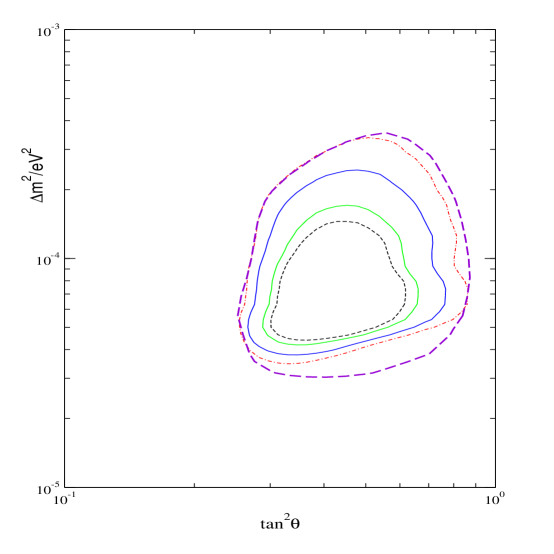
Figure 1: The 90%, 95%, 99% and 99.73%($3\sigma$) C.L. contours from a $\chi^{2}$ analysis using KamLAND rate + global solar data. The dashed line shows the presently allowed $3\sigma$ solar contour.

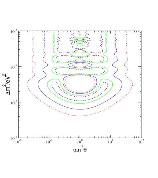
Figure 2: The 90%, 95%, 99% and 99.73%($3\sigma$) C.L. contours from a $\chi^{2}$ analysis using the KamLAND spectrum data.

The $\chi^{2}$ for the combined solar and KamLAND rate analysis is defined as

$$\chi^{2}=\chi^{2}_{\odot}+\chi^{2}_{KL}$$ (6)

The best-fit after including the KamLAND data comes at $\Delta m^{2}=6.06\times 10^{-5}$ eV² and $\tan^{2}\theta=0.42$. Thus the best-fit point does not change significantly with respect to that obtained from only solar analysis [12]. In Figure 1 we draw the 90%, 95%, 99% and 99.73% C.L. allowed area in the LMA region from a combined solar+KamLAND rate analysis. Superimposed on that we show the $3\sigma$ (99.73% C.L.) allowed area from solar data alone. Large area within the LMA regions is seen to remain allowed.

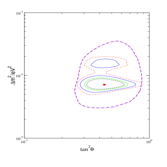
Figure 3: The 90%, 95%, 99% and 99.73% C.L. contours from a $\chi^{2}$ analysis using KamLAND spectrum data along with global solar data. The dashed line shows the presently allowed $3\sigma$ only solar contour.

Data	$\Delta m^{2}$	$\tan^{2}\theta$	$\chi^{2}_{min}$
Used	in eV2
	$7.17\times 10^{-5}$	$0.64$	5.71
KamLAND	$1.50\times 10^{-4}$	0.34	8.24
	$7.17\times 10^{-5}$	0.43	74.39
KamLAND + Solar	$1.48\times 10^{-4}$	0.44	81.51

Table 1: The $\chi^{2}_{min}$ and the best-fit values of the oscillation parameters obtained from the analysis of the KamLAND spectrum data alone and from the global analysis of the KamLAND spectrum data and the solar neutrino data.

Apart from the data on energy integrated total rates, KamLAND collaboration has also provided the observed positron visible energy spectrum, albeit with low statistics. We incorporate this in our analysis to extract the shape information from this data as the spectral distortion is a very sensitive probe of $\Delta m^{2}$. For the KamLAND spectral data, we perform our analysis using a definition of $\chi^{2}_{klspec}$ assuming the data to be Poisson-distributed which is appropriate for data with low statistics. For this case

$$\chi^{2}_{klspec}=\sum_{i}\left[2(X_{n}S_{KL,i}^{theory}-S_{KL,i}^{expt})+2S_{KL,i}^{expt}\ln(\frac{S_{KL,i}^{expt}}{X_{n}S_{KL,i}^{theory}})\right]+\frac{(X_{n}-1)^{2}}{\sigma^{2}_{sys}}$$ (7)

where $\sigma_{sys}$ is taken to be 6.42% [1] and a normalisation factor $X_{n}$ is allowed to vary freely. The sum is over the 13 KamLAND spectral bins. In [1] the errors for the shape distortion are attributed to energy scale, energy resolution, $\bar{\nu}_{e}$ spectrum and fiducial volume. A more refined statistical analysis would involve evaluating the systematic errors in each bin due to these sources at each $\Delta m^{2}$ and $\tan^{2}\theta$ as well as taking into account of the background events and their errors in each bin. This will be possible as and when more detailed information will be available.

For the spectrum analysis we get the best-fit values of $\Delta m^{2}$ and $\tan^{2}\theta$ to be $7.17\times 10^{-5}$ eV² and 0.64 respectively. This is close to that obtained by the KamLAND collaboration but our best-fit $\theta$ is not maximal as in [1]. Apart from the above there are other minimas with reduced statistical significance. In Table 1 we present the best-fit values and $\chi^{2}_{min}$ for the global minima and the second minima which is obtained at a higher $\Delta m^{2}$ value. In Figure 2 we present the allowed areas in $\Delta m^{2}-\tan^{2}\theta$ plane from KamLAND spectrum analysis. This is understandably slightly different from what KamLAND has obtained in [1]. The KamLAND data analysis procedure as outlined in [1] is somewhat different and the full details are not known to us.

Next we do a combined analysis of KamLAND spectral data together with the global solar data. The $\chi^{2}$ for the combined analysis is defined as the sum of the individual contributions. We present the results in Table 1. The best-fit comes at $\Delta m^{2}=7.17\times 10^{-5}$ eV² and $\tan^{2}\theta=0.43$. From Table 1 we also see that there is a second minima at a higher $\Delta m^{2}$ with a reduced statistical significance by about 2$\sigma$ with respect to (w.r.t.) the global minima.

In Figure 3 we show the combined allowed area with the solar and KamLAND spectrum analysis superimposed on the 3$\sigma$ solar contour. The allowed area is seen to be much constricted with the inclusion of the KamLAND spectral data. At 90% C.L. only a small region about the best-fit point remains allowed. At 99% C.L. however there are two distinct allowed zones – one around the global best-fit point (low-LMA) and the other around the higher $\Delta m^{2}$ corresponding to the second minima (high-LMA). The former is preferred by the KamLAND data and to a greater extent by the global solar data. At 99.73% the demarkation between the two zones disappear.

In Table 2 we show the allowed ranges of the values of the parameters at 99% C.L. obtained from the global analysis including the solar and KamLAND spectrum data. The allowed range of $\tan^{2}\theta$ is not reduced in the preferred low-LMA zone with the inclusion of KamLAND data, although in the high-LMA zone it is somewhat restricted.

Allowed	99% C.L. Range of	99% C.L. Range of
Zone	$\Delta m^{2}$ in eV2	$\tan^{2}\theta$
low-LMA	$5.3\times 10^{-5}<\Delta m^{2}<9.9\times 10^{-5}$	$0.28<\tan^{2}\theta<0.79$
high-LMA	$1.3\times 10^{-4}<\Delta m^{2}<1.8\times 10^{-4}$	$0.34<\tan^{2}\theta<0.55$

Table 2: Range of parameter values allowed at 99% C.L. from the global solar and KamLAND spectrum analysis.

For the LOW solution we get $\chi^{2}_{min}=97.28$. This implies that LOW is now ruled out at 4.4$\sigma$ w.r.t. the LMA solution. The maximal mixing solution ($\chi^{2}_{min}=88.89$) is disfavored at 3.4$\sigma$ (w.r.t. LMA) from the combined KamLAND + solar analysis.

3 Projected Analysis

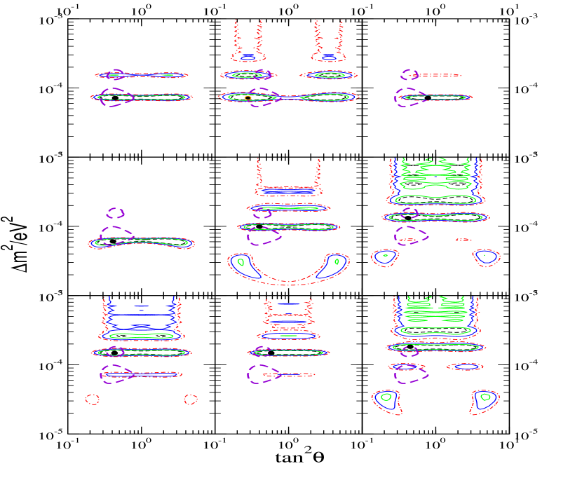
Figure 4: The 90%, 95%, 99% and 99.73% C.L. contours for using the 1 kton-yr projected KamLAND spectrum. The different panels are for the simulated spectrum at values of $\Delta m^{2}$ and $\tan^{2}\theta$ indicated by the black dots. The dashed line shows the currently allowed 99% C.L. contour from solar+KamLAND analysis.

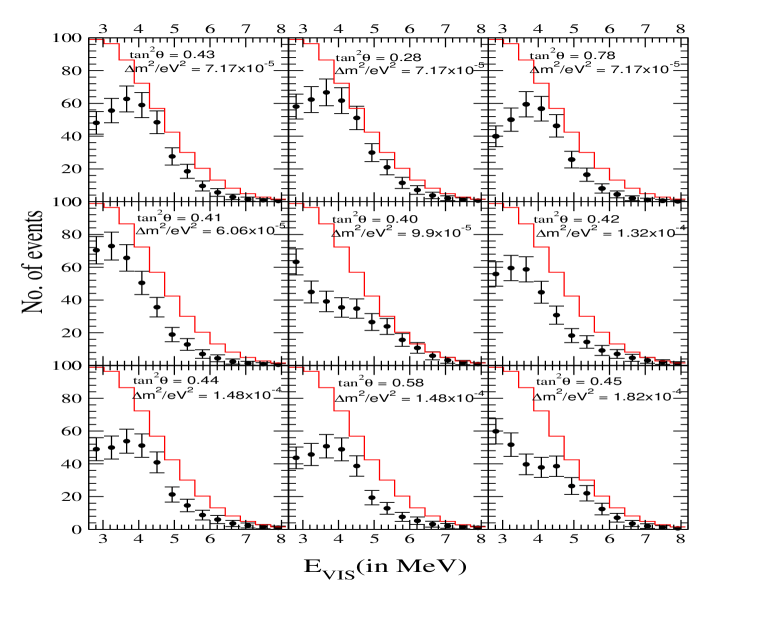
Figure 5: The 1 kton-yr simulated KamLAND spectrum for the different sets of $\Delta m^{2}$ and $\tan^{2}\theta$ corresponding to Figures 4 and 6. The histogram shows the unoscillated spectrum for 1 kton-yr.

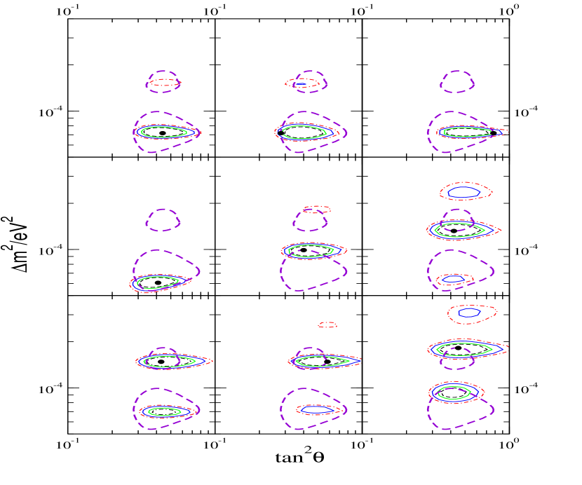
Figure 6: Same as in Figure. 4 but from a combined analysis using the solar+CHOOZ+1 kton-yr projected KamLAND spectrum data. Since the solar data disfavour the $\theta>\pi/4$ regions this figure is plotted with $\tan^{2}\theta$ extending upto 1.0.

In this section we explore whether the future KamLAND spectrum data would be able to determine the allowed zones more precisely. In particular, it would be interesting to see whether KamLAND , either by itself or in conjunction with the solar data, can choose between one of the two allowed islands, and pin down the values of the mass and mixing parameters unambiguously. We try to look into this by doing a statistical analysis of the projected 1 kton-yr KamLAND data. We choose sample values of $\Delta m^{2}$ and $\tan^{2}\theta$, from the allowed zones obtained from the global solar+KamLAND analysis (cf. fig.3) and simulate the spectrum at these points for 1 kton-yr of data (approximately 2.5 years of KamLAND live-time ), using a randomizing procedure which takes care of the fluctuations. We use these simulated spectra in a $\chi^{2}$ analysis and reconstruct the allowed regions in the $\Delta m^{2}$–$\tan^{2}\theta$ plane. In Figure 4 we display these reconstructed allowed regions from 1 kton-yr projected KamLAND spectrum alone. Figure 5 shows the 1 kton-yr simulated spectrum with errorbars at the $\Delta m^{2}$ and $\tan^{2}\theta$ corresponding to each of the panels of Figure 4. In Figure 6 we present the allowed regions from a combined analysis of global solar data and 1 kton-yr KamLAND spectrum data, simulated at the same set of points as in the previous two figures. The dashed lines in Figures 4 and 6 give the current 99% C.L. allowed regions. For the analysis with the projected KamLAND spectra we assume Gaussian statistics, which is more appropriate in this case.

First let us make a note on the rationale of the representative values of $\Delta m^{2}$ and $\tan^{2}\theta$ chosen to simulate the spectrum. Panel 1 corresponds to the KamLAND spectrum simulated at the low-LMA best-fit while panel 7 corresponds to that generated at the high-LMA best-fit. These are the two favored points from the current data. We also simulate the 1 kton-yr KamLAND spectrum at few other points deviated from the best-fits. In panel 2(3) we have chosen $\Delta m^{2}$ corresponding to the low-LMA best-fit but a lower(higher) value of $\theta$. Similarly panel 8 is for $\Delta m^{2}$ corresponding to the high-LMA best fit but at a higher value of $\theta$. The panels with same $\Delta m^{2}$ but different $\theta$ are chosen to demonstrate the impact of $\theta$ on the reconstructed regions. We choose $\Delta m^{2}$ values lower(higher) than the low(high)-LMA best-fit in panels 4(5). Panels 6 and 8 display the reconstructed regions for $\Delta m^{2}$ values lower and higher than the high-LMA best-fit respectively. These set of values give adequate coverage for studying the projected sensitivity of the reconstructed regions on the choice of $\Delta m^{2}$ and $\theta$ currently allowed at 99% C.L..

Figure 4 addresses the issue if future KamLAND data can by itself make a sharper demarkation between the two allowed islands and the dependence of this on the oscillation parameters. The figure shows that if we choose the simulation point at higher $\Delta m^{2}$ values (panels 5, 6, 7, 8 and 9) then there are large allowed regions from the spectrum data, extending upto $10^{-3}$ eV². The Figure 5 shows that for these values of $\Delta m^{2}$ the spectral suppression tends to become flat (undistorted) leading to increased fuzziness. The same is also true for lower values of $\theta$. The lesser distortion at low values of $\tan^{2}\theta$ is due to a diminished energy dependence resulting from a small oscillatory term in the survival probability [23]. This also leads to an increase in allowed area (cf. panel 2) although to a lesser extent as compared to the panels with high $\Delta m^{2}$ values discussed earlier. There are also some allowed regions at $\Delta m^{2}$ values lower than that allowed by the current 99% C.L. contour in panels 5, 6, 7 and 9. However the figure reveals that the allowed $\Delta m^{2}$ range around the low-LMA and high-LMA zones get reduced in most of the panels. With 1 kton-yr KamLAND spectrum data the region around $\Delta m^{2}\sim 10^{-4}$ eV² present in Figure 3 gets disallowed in all the panels and the low-LMA and high-LMA regions get bifurcated even at 3$\sigma$ level. In general, tighter constraints in the Figure 4 are associated with spectra with a shape significantly different from the no oscillation spectrum. For the KamLAND baselines this corresponds to a lower $\Delta m^{2}$ than the present best-fit. Panel 4, which is at the global solar best-fit, shows that for such cases just the 1 kton-yr spectrum data from KamLAND can pick out a sharply defined allowed zone around the simulation point unambiguously.

In Figure 6 we show the C.L. allowed regions from a combined analysis of the global solar + CHOOZ + 1 kton-yr KamLAND simulated spectrum data. Through these plots we investigate the impact of the current solar data to resolve the ambiguity still admitted by the 1 kton-yr projected KamLAND spectrum data. We find that the solar data is instrumental in ruling out a large part of the parameter space allowed by the 1 kton-yr KamLAND only analysis. A comparison of the panels 1, 2, 3 and 5 in the figures 4 and 6 shows that for spectrum simulated in the low-LMA region the inclusion of the solar data reduces the statistical significance of the high-LMA zone. It also disallows the high $\Delta m^{2}$ regions above $2\times 10^{-4}$ eV². In these regions the solar data requires a ${}^{8}{B}$ flux normalisation factor ($f_{B}$) $\sim$ 0.8 which is in conflict with the SNO NC measurement of $f_{B}\sim 1.0$, thus disfavoring these zones. For spectrum simulated in the high-LMA region in panels 6 to 9, even though the large allowed regions beyond $2\times 10^{-4}$ eV² as well as the allowed regions at low $\Delta m^{2}$ get mostly removed by the solar data, the ambiguity between the allowed islands remain. In fact a comparison with Figure 4 reveals that for these panels the inclusion of the solar data increases the statistical significance of the low-LMA allowed regions. The KamLAND spectral data allows the low-LMA region only at 99% C.L. in panels 7, 8 and 9, and at 99.73% C.L. in panel 6. However with the inclusion of the solar data in the analysis, these regions become allowed at 90% and 99% C.L. respectively, as the solar data prefers the low-LMA zone. Therefore to remove the ambiguity for the spectrum corresponding to the high-LMA zones, one would require KamLAND data with higher statistics, which will be able to determine the spectral shape and hence $\Delta m^{2}$ more precisely.

4 Conclusions

In conclusion, we have investigated the impact of the first results from KamLAND on neutrino mass and mixing parameters in conjunction with the global solar neutrino data. KamLAND is completely consistent with the LMA solution, to the extent that the observed KamLAND rate is close to that predicted by the best-fit point of the LMA solution to the solar neutrino problem. As a result the combined analysis of the solar and KamLAND rates data allows a large area within the solar LMA region and the global solar best-fit does not change much with inclusion of KamLAND rates. The constraining capabilities of the spectrum data is much stronger and with only 145 days observed spectrum KamLAND can exclude certain parts of the LMA parameter space. After including the spectral data the allowed LMA zone consists mainly of two disconnected regions, one around the best-fit and another at a higher $\Delta m^{2}$. The two zones merge at $3\sigma$. Maximal mixing though allowed by the KamLAND alone, is found to be still disfavored by the combined solar and KamLAND data at more than $3\sigma$. The LOW solution which was allowed at $3\sigma$ from the global solar data and which predicts null oscillations in KamLAND is now disfavored at almost $5\sigma$ w.r.t the LMA solution.

With LMA now confirmed, the next focus of KamLAND would be a more accurate determination of the mass parameter by distinguishing between the two allowed sectors in the LMA region. We have explored this through a projected analysis with 1 ktyr simulated data. With 1 kton-yr projected spectrum data the allowed $\Delta m^{2}$ ranges around both low-LMA and high-LMA zones decrease in size and they get separated at 3$\sigma$ by the spectrum data itself. The inclusion of the solar data disfavours(favours) the high(low)-LMA zone if the spectrum is simulated in the low(high)-LMA area. Thus the allowed areas become more precise for low-LMA spectrum while ambiguity between the two zones remains for high-LMA spectrum. A higher statistics from KamLAND is expected to resolve this ambiguity. A more precise determination of the mixing angle will be possible from a more accurate measurement of the CC/NC ratio at SNO.

Acknowledgment We acknowledge S. Pakvasa for useful discussions. RG would like to thank John Beacom for a helpful discussion. SC acknowledges discussions with S.T. Petcov.

References

- [1] K. Eguchi et al. [KamLAND Collaboration], Phys. Rev. Lett. 90, 021802 (2003) [arXiv:hep-ex/0212021].
- [2] B. T. Cleveland et al., Astroph. J. 496 (1998) 505.
- [3] J. N. Bahcall, M.H. Pinsonneault and S. Basu, Astrophys. J. 555 (2001)990.
- [4] T. Kirsten, talk at Neutrino 2002, XXth International Conference on Neutrino Physics and Astrophysics, Munich, Germany, May 25-30, 2002. (http://neutrino2002.ph.tum.de/); See also J.N. Abdurashitov et al., . Exp. Theor. Phys. 95, 181 (2002) [Zh. Eksp. Teor. Fiz. 122, 211 (2002)] [arXiv:astro-ph/0204245].
- [5] V. Gavrin, talk at Neutrino 2002, XXth International Conference on Neutrino Physics and Astrophysics, Munich, Germany, May 25-30, 2002. (http://neutrino2002.ph.tum.de/)
- [6] S. Fukuda et al. [Super-Kamiokande Collaboration], Phys. Lett. B 539, 179 (2002) [arXiv:hep-ex/0205075].
- [7] Q. R. Ahmad et al. [SNO Collaboration], Phys. Rev. Lett. 89, 011301 (2002) [arXiv:nucl-ex/0204008].
- [8] Q. R. Ahmad et al. [SNO Collaboration], Phys. Rev. Lett. 89, 011302 (2002) [arXiv:nucl-ex/0204009].
- [9] L. Wolfenstein, Phys. Rev. D34, 969 (1986); S.P. Mikheyev and A.Yu. Smirnov, Sov. J. Nucl. Phys. 42(6), 913 (1985); Nuovo Cimento 9c, 17 (1986).
- [10] V. Barger, D. Marfatia, K. Whisnant and B. P. Wood, Phys. Lett. B 537, 179 (2002) [arXiv:hep-ph/0204253].
- [11] A. Bandyopadhyay, S. Choubey, S. Goswami and D. P. Roy, Phys. Lett. B 540, 14 (2002) [arXiv:hep-ph/0204286].
- [12] S. Choubey, A. Bandyopadhyay, S. Goswami and D. P. Roy, arXiv:hep-ph/0209222.
- [13] A. Bandyopadhyay, S. Choubey and S. Goswami, Phys. Lett. B 555, 33 (2003) [arXiv:hep-ph/0204173].
- [14] J. N. Bahcall, M. C. Gonzalez-Garcia and C. Pena-Garay, JHEP 0207, 054 (2002) [arXiv:hep-ph/0204314].
- [15] P. Creminelli, G. Signorelli A. Strumia, hep-ph/0102234, v3 22 April 2002 (addendum 2).
- [16] P. Aliani, V. Antonelli, R. Ferrari, M. Picariello and E. Torrente-Lujan, Phys. Rev. D 67, 013006 (2003) [arXiv:hep-ph/0205053].
- [17] P. C. de Holanda and A. Y. Smirnov, Phys. Rev. D 66, 113005 (2002) [arXiv:hep-ph/0205241].
- [18] A. Strumia, C. Cattadori, N. Ferrari and F. Vissani, Phys. Lett. B 541, 327 (2002) [arXiv:hep-ph/0205261].
- [19] G. L. Fogli, E. Lisi, A. Marrone, D. Montanino and A. Palazzo, Phys. Rev. D 66, 053010 (2002) [arXiv:hep-ph/0206162].
- [20] M. Maltoni, T. Schwetz, M. A. Tortola and J. W. Valle, Phys. Rev. D 67, 013011 (2003) [arXiv:hep-ph/0207227].
- [21] P. Alivisatos et al., KamLAND, Stanford-HEP-98-03, Tohoku-RCNS-98-15. J. Busenitz et. al, “Proposal for US Participation in KamLAND”, March 1999, ( http://bfk1.lbl.gov/KamLAND/).
- [22] P. Vogel and J. F. Beacom, Phys. Rev. D 60, 053003 (1999) [arXiv:hep-ph/9903554].
- [23] A. Bandyopadhyay, S. Choubey, R. Gandhi, S. Goswami and D. P. Roy, arXiv:hep-ph/0211266.
- [24] V. D. Barger, D. Marfatia and B. P. Wood, Phys. Lett. B 498, 53 (2001) [arXiv:hep-ph/0011251].
- [25] H. Murayama and A. Pierce, Phys. Rev. D 65 (2002) 013012 [arXiv:hep-ph/0012075].
- [26] A. de Gouvea and C. Pena-Garay, Phys. Rev. D 64, 113011 (2001) [arXiv:hep-ph/0107186].
- [27] A. Strumia and F. Vissani, JHEP 0111, 048 (2001) [arXiv:hep-ph/0109172].
- [28] M. C. Gonzalez-Garcia and C. Pena-Garay, Phys. Lett. B 527, 199 (2002) [arXiv:hep-ph/0111432].
- [29] P. Aliani, V. Antonelli, M. Picariello and E. Torrente-Lujan, New J. Phys. 5, 2 (2003) [arXiv:hep-ph/0207348].
- [30] G. L. Fogli, G. Lettera, E. Lisi, A. Marrone, A. Palazzo and A. Rotunno, Phys. Rev. D 66, 093008 (2002) [arXiv:hep-ph/0208026].
- [31] M. Apollonio et al. [CHOOZ Collaboration], Phys. Lett. B 420, 397 (1998) [arXiv:hep-ex/9711002]; M. Apollonio et al. [CHOOZ Collaboration], Phys. Lett. B 466, 415 (1999) [arXiv:hep-ex/9907037].