We investigate $\overline{B^{0}}\rightarrow D_{s}^{-}\pi^{+}$ decay in perturbative QCD approach which has recently been applied to $B$ meson decays. $\overline{B^{0}}\rightarrow D_{s}^{-}\pi^{+}$ decay (and its charge conjugated mode) can be one of the hopeful modes to determine $|V_{ub}|$ since it occurs through $b\rightarrow u$ transition only. We estimate both factorizable and non-factorizable contribution, and show that the non-factorizable contribution is much less than the factorizable one. Our calculation gives $\mbox{BR}(\overline{B^{0}}\rightarrow D_{s}^{-}\pi^{+})=(50\sim 70)\times f_{Ds}^{2}|{V_{ub}}{V_{cs}}|^{2}$.

Keywords: KM matrix; $V_{ub}$; non-leptonic B decay; pQCD approach.

PACS Nos. : 12.15.Hh, 12.38.Bx, 12.39.St, 13.25.Hw

The determination of all the elements of Kobayashi-Maskawa matrix [1] is important for the consistency check of the standard model and a search for new physics. Much extensive experimental efforts have been being done at $B$ meson dedicated facilities (B factories) to complete the determination of KM matrix elements to third generation. $|V_{cb}|$ has well been determined owing to heavy quark symmetry[2] to the accuracy of less than 10 % error. But $|V_{ub}|$ has not yet been determined so precisely[3]. The experimental error will be greatly reduced by the coming experiments in the very near future, while we need more effort to reduce the theoretical uncertainty. It is mainly due to hadronic effects which we do not yet have an precise method to calculate.

So far $b\rightarrow u$ semi-leptonic decays have been mainly used for the experimental determination of $|V_{ub}|$. It is interesting to investigate other modes involving non-leptonic decays to extract $|V_{ub}|$ for the consistency checks of the experimental value of $|V_{ub}|$ and the theoretical methods to estimate hadronic effects. More experimental information can be available and we can tune up the theoretical methods. We propose here $\overline{B^{0}}\rightarrow D_{s}^{-}\pi^{+}$ decay as one of good candidates to investigate. The final state $D_{s}^{-}\pi^{+}$ is composed of $(s\bar{c})$ $(u\bar{d})$ quark state. The $b$ quark in $\overline{B^{0}}$ meson cannot directly decay into $\bar{c}$ quark by $W^{-}$ emission as the color quantum number is different. Also no penguin, exchange nor annihilation contributions exist since no $q\bar{q}$ state presents in the final state. Therefore, the decay occurs through $b\rightarrow u$ transition only, which makes $\overline{B^{0}}\rightarrow D_{s}^{-}\pi^{+}$ a good mode to determine $|V_{ub}|$.

$\overline{B^{0}}\rightarrow D_{s}^{-}\pi^{+}$ and its charge conjugate mode are hopeful from experimental point of view also. Both $D_{s}$ and charged pion are relatively easy to be identified in the present experiments. Recently, BABAR and BELLE groups obtained the branching ratio, BR$(B^{0}\rightarrow D_{s}^{+}\pi^{-})=3.2\pm 0.9\pm 1.0\times 10^{-5}$ (BABAR) [4], $2.4{\scriptsize\begin{array}[]{l}+1.0\\ -0.8\end{array}}\pm 0.7\times 10^{-5}$ (BELLE) [5]. With increasing statistics at B factories we can expect that the branching ratio is fixed more precisely in the very near future.

The $\overline{B^{0}}\rightarrow D_{s}^{-}\pi^{+}$ decay occurs through the effective Hamiltonian,

$${\cal H}_{eff} = \frac{G_{F}}{\sqrt{2}}{V_{ub}}{V_{cs}}^{*}[c_{1}(\bar{s}b)_{V-A}(\bar{u}c)_{V-A}+c_{2}(\bar{u}b)_{V-A}(\bar{s}c)_{V-A}]+\mbox{(h.c.)}$$ (1)

$$\equiv \frac{G_{F}}{\sqrt{2}}{V_{ub}}{V_{cs}}^{*}[c_{1}O_{1}+c_{2}O_{2}]+\mbox{(h.c.)},$$ (2)

where $c_{1,2}$ are the Wilson coefficients obtained by solving renormalization group equations, and $O_{1,2}$ are 4-quark operators[6]. We need to estimate $\langle D_{s}^{-}\pi^{+}|O_{1,2}|\overline{B^{0}}\rangle$ to obtain the branching ratio theoretically. So far, factorization ansatz[7] has often been used to estimate this kind of 2-body decay hadron matrix elements;

$$A[\overline{B^{0}}\rightarrow D_{s}^{-}\pi^{+}] \simeq \frac{G_{F}}{\sqrt{2}}{V_{ub}}{V_{cs}}^{*}\left(c_{2}+\frac{c_{1}}{N_{eff}}\right)\langle D_{s}^{-}(P_{2})|(\bar{s}c)_{V-A}|0\rangle\langle\pi^{+}(P_{3})|(\bar{u}b)_{V-A}|\overline{B^{0}}(P_{1})\rangle$$ (3)

$$= if_{Ds}\frac{G_{F}}{\sqrt{2}}{V_{ub}}{V_{cs}}^{*}\left(c_{2}+\frac{c_{1}}{N_{eff}}\right)M_{B}^{2}F_{0}({M_{Ds}}^{2}),$$

where $N_{eff}$ is the effective color number and $f_{Ds}$ is the $D_{s}$ meson decay constant. Pion mass is neglected. The $B\rightarrow\pi$ transition form factors are defined as follows;

$$\langle\pi^{+}(P_{3})|\bar{u}\gamma_{\mu}b|\overline{B^{0}}(P_{1})\rangle\equiv\left[(P_{1}+P_{3})_{\mu}-\left(\frac{M_{B}^{2}}{q^{2}}\right)q_{\mu}\right]F_{1}(q^{2})+\left(\frac{M_{B}^{2}}{q^{2}}\right)q_{\mu}F_{0}(q^{2}),$$ (4)

where $q=P_{1}-P_{3}$. Form factors are to be obtained from another theory or experimental data. The deviation of $N_{eff}$ from the number of color, $N_{C}=3$, accounts for so-called non-factorizable contributions. With the amplitude given by eq.(3) the $\overline{B^{0}}\rightarrow D_{s}^{-}\pi^{+}$ branching ratio is calculated as

$$\mbox{BR}(\overline{B^{0}}\rightarrow D_{s}^{-}\pi^{+})=\tau(\overline{B^{0}})\frac{(1-r^{2})}{32\pi}G_{F}^{2}M_{B}^{3}\left(c_{2}+\frac{c_{1}}{N_{eff}}\right)^{2}F_{0}(M_{Ds})^{2}f_{Ds}^{2}|V_{ub}V_{cs}|^{2},$$ (5)

where $r\equiv M_{Ds}/M_{B}$. Below we first give estimations of the branching ratio based on the factorization ansatz by using the $B\rightarrow\pi$ transition form factor from light-cone sum rules and lattice QCD. Then we calculate ${\overline{B^{0}}}\rightarrow D_{s}^{-}\pi^{+}$ amplitude by using perturbative QCD (pQCD) approach to estimate non-factorizable contribution. pQCD approach has been applied to estimate pion electro-magnetic form factor, $B\rightarrow D$, $B\rightarrow\pi$ transition form factors and several decay amplitudes of 2-body decays of B meson ($D\pi$, $\pi\pi$, $K\pi$ and $K^{*}\gamma$) [8]. The results of pQCD approach nicely agree with experimental data. The advantage of pQCD approach lies in the point that the non-factorizable contribution can be calculated based on well-established perturbative QCD technique for heavy meson decays. We show that the non-factorizable contribution is about 10% or less of the factorizable one in $B\rightarrow D_{s}\pi$, so that naive factorization estimation gives a reasonable prediction for this decay mode.

In the evaluation of eq.(5) we consider the Wilson coefficients at two scales, $\mu=M_{B}$ and $M_{B}/2$, to estimate the ambiguity coming from the choice of the scale;

$\mu$	$M_{B}$	$M_{B}/2$
$c_{1}(\mu)$	$-0.274$	$-0.393$
$c_{2}(\mu)$	$1.12$	$1.19$

The $B\rightarrow\pi$ transition form factor based on light-cone sum rules calculation can be parametrized as

$$F_{0}(q^{2})=\frac{F_{0}(0)}{1-a_{F}(q^{2}/M_{B}^{2})+b_{F}(q^{2}/M_{B}^{2})^{2}}$$ (6)

with $F_{0}(0)=0.305$, $a_{F}=0.266$ and $b_{F}=-0.752$ [10]. With the calculation by lattice QCD[11] we make a fit for $B\rightarrow\pi$ transition form factor as

$$F_{0}(q^{2})=\frac{F_{0}(0)}{1-c_{F}(q^{2}/M_{B}^{2})}$$ (7)

with $F_{0}(0)=0.310$, $c_{F}=0.760$. The estimated value of $\mbox{BR}(\overline{B^{0}}\rightarrow D_{s}^{-}\pi^{+})/(f_{Ds}^{2}|V_{ub}V_{cs}|^{2})$ is given in Table 1.

	$\begin{array}[]{c}N_{eff}=3\\ \mu=M_{B}\end{array}$	$\begin{array}[]{c}N_{eff}=2\\ \mu=M_{B}\end{array}$	$\begin{array}[]{c}N_{eff}=3\\ \mu=M_{B}/2\end{array}$	$\begin{array}[]{c}N_{eff}=2\\ \mu=M_{B}/2\end{array}$
lattice $F_{0}$	51.1	46.7	53.9	47.4
sum rules $F_{0}$	44.0	40.1	46.4	40.8

Table 1: $\mbox{BR}(\overline{B^{0}}\rightarrow D_{s}^{-}\pi^{+})/(f_{Ds}^{2}|V_{ub}V_{cs}|^{2})$

By adopting $f_{Ds}=0.241\pm 0.032$ GeV obtained by taking average of several experimental data[12], we can summarize the naive factorization estimation as

$$\mbox{BR}(\overline{B^{0}}\rightarrow D_{s}^{-}\pi^{+})/|V_{ub}V_{cs}|^{2}=\left\{\begin{array}[]{cl}2.0\sim 4.0&\mbox{(lattice $F_{0}$)}\\ 1.8\sim 3.5&\mbox{(sum rules $F_{0}$)}\end{array}\right..$$ (8)

The ambiguity from the choice of $N_{eff}$ and $\mu$ is about 10% and 5%, respectively. The major ambiguity lies in $f_{Ds}$ value.

There are factorizable and non-factorizable contribution in $\overline{B^{0}}\rightarrow D_{s}^{-}\pi^{+}$. When a gluon connects the spectator $\bar{d}$ quark and a quark in $D_{s}$ meson in Fig.1, the contribution cannot be factorized as in eq.(3).

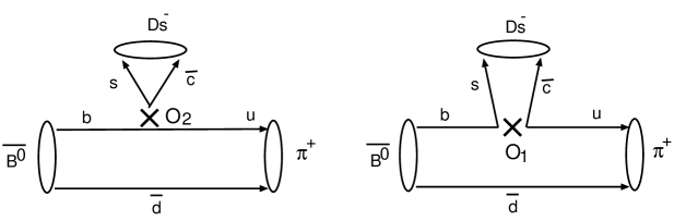
Figure 1: Diagrams contributing to $\overline{B^{0}}\rightarrow D_{s}^{-}\pi^{+}$. Gluon is not shown.

The non-factorizable contribution is taken into account by changing the color number from $N_{C}=3$ to $N_{eff}$ in the calculation based on the factorization ansatz. However, the number to be taken as $N_{eff}$ is theoretically unclear. We have to rely on fit of $N_{eff}$ by using experimental data other than $B\rightarrow D_{s}\pi$. But, we cannot simply adopt the $N_{eff}$ in other decays because the topology of diagrams contributing to other decays is not necessary same as in the case of $\overline{B^{0}}\rightarrow D_{s}^{-}\pi^{+}$ decay. Here we calculate $\overline{B^{0}}\rightarrow D_{s}^{-}\pi^{+}$ amplitude in pQCD approach[8] to estimate the non-factorizable contribution based on QCD.

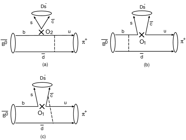
Figure 2: Some diagrams contributing to $\overline{B^{0}}\rightarrow D_{s}^{-}\pi^{+}$ in pQCD. Gluon is shown in dashed line.

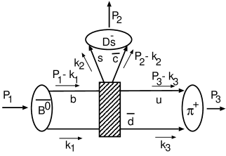
Figure 3: Momentum flow in the diagrams contributing to $\overline{B^{0}}\rightarrow D_{s}^{-}\pi^{+}$ in pQCD.

Some of representative diagrams contributing to $\overline{B^{0}}\rightarrow D_{s}^{-}\pi^{+}$ in pQCD approach is shown in Fig.2. The point is that in 2 body decays of $B$ meson the spectator quark has to obtain high momentum to form a meson with one of the emitted rapid quarks from $b$ quark decay. The high momentum is carried by a gluon, so the perturbative QCD treatment is possible. The non-perturbative nature is put into meson wave functions. For more details refer the papers in [8]. There is another approach of calculating non-leptonic 2-body decays of B meson by using perturbative QCD, the so-called QCD factorization method[9]. One of the major differences between pQCD approach and QCD factorization lies in the treatment of the transverse momentum. It is taken into account in the pQCD approach while neglected in the QCD factorization. Without the transverse momentum the diagrams given in fig.2 have infrared singularities which makes the results of the calculation implausible. The calculation based on pQCD approach can be done in a similar way to calculate $B\rightarrow D\pi$ amplitude given in Li and Melić[8]. The assignment of momenta is shown in Fig.3 where $P_{1}=(M_{B}/\sqrt{2})\>(1,1,0_{T})$, $P_{2}=(M_{B}/\sqrt{2})\>(r^{2},1,0_{T})$, $P_{3}=(M_{B}/\sqrt{2})\>(1-r^{2},1,0_{T})$ and $k_{1}=(0,x_{1}(M_{B}/\sqrt{2}),k_{1T})$, $k_{2}=(0,x_{2}(M_{B}/\sqrt{2}),k_{2T})$, $k_{3}=(x_{3}(1-r^{2})(M_{B}/\sqrt{2}),0,k_{3T})$ in light-cone coordinate. We obtain

$$\Gamma[\overline{B^{0}}\rightarrow D_{s}^{-}\pi^{+}]=\frac{G_{F}^{2}}{128\pi}|V_{ub}V_{cs}|^{2}M_{B}^{3}\frac{(1-r^{2})^{3}}{r}|f_{Ds}\xi_{\rm int}+{\cal M}_{\rm int}|^{2}.$$ (9)

The factorizable contribution, $f_{Ds}\xi_{\rm int}$, is given as

$$\xi_{\rm int} = 16\pi C_{F}\sqrt{r}M_{B}^{2}\int_{0}^{1}dx_{1}dx_{3}\int_{0}^{1/\Lambda}b_{1}db_{1}b_{3}db_{3}\phi_{B}(x_{1},b_{1})$$ (10)

$$\times\alpha_{s}(t_{\rm int})\left(c_{2}(t_{\rm int})+\frac{c_{1}(t_{\rm int})}{N_{C}}\right)\exp[-S_{B}(t_{\rm int})-S_{\pi}(t_{\rm int})]$$

$$\times\Biggl{[}[\{1+x_{3}(1-r^{2})\}\phi_{A}(x_{3})+r_{0}\{\left(\frac{1+r^{2}}{1-r^{2}}\right)-2x_{3}\}\phi_{P}(x_{3})$$

$$\ \ \ \ \ -r_{0}(2x_{3}-1)\phi_{T}(x_{3})]h(x_{1},x_{3},b_{1},b_{3},m_{\rm int})$$

$$\ \ +[x_{1}r^{2}\phi_{A}(x_{3})+2r_{0}\{1-\left(\frac{r^{2}}{1-r^{2}}\right)x_{1}\}\phi_{P}(x_{3})]h(x_{3},x_{1},b_{3},b_{1},m_{\rm int})\Biggr{]}\;,$$

where $\exp[-S_{B}(t_{\rm int})-S_{\pi}(t_{\rm int})]$ is Sudakov factor[8], $m_{\rm int}=(1-r^{2})M_{B}^{2}$, $\Lambda=\Lambda_{\rm QCD}$ and $t_{\rm int}={\rm max}(\sqrt{x_{1}m_{\rm int}},\sqrt{x_{3}m_{\rm int}},1/b_{1},1/b_{3})$. The parameter $b_{i}$ ($i=1\sim 3$) is the conjugate variable of $k_{iT}$. The function $h(x_{1},x_{3},b_{1},b_{3},m)$ is defined as

$$h(x_{1},x_{3},b_{1},b_{3},m) = S_{t}(x_{3})K_{0}\left(\sqrt{x_{1}x_{3}m}b_{1}\right)$$ (11)

$$\times\left[\theta(b_{1}-b_{3})K_{0}\left(\sqrt{x_{3}m}b_{1}\right)I_{0}\left(\sqrt{x_{3}m}b_{3}\right)\right.$$

$$\ \ \ \left.+\theta(b_{3}-b_{1})K_{0}\left(\sqrt{x_{3}m}b_{3}\right)I_{0}\left(\sqrt{x_{3}m}b_{1}\right)\right],$$

where

$$S_{t}(x)=\frac{2^{1+2c}\Gamma(c+3/2)}{\sqrt{\pi}\Gamma(c+1)}[x(1-x)]^{c}\ \ (c=0.3\sim 0.4),$$ (12)

which comes from threshold resummation[13]. The non-factorizable contribution is given as

$${\cal M}_{\rm int} = -32\pi\sqrt{2N_{C}}C_{F}\sqrt{r}M_{B}^{2}\int_{0}^{1}dx_{1}dx_{2}dx_{3}\int_{0}^{1/\Lambda}b_{1}db_{1}b_{2}db_{2}\phi_{B}(x_{1},b_{1})\phi_{Ds}(x_{2},b_{2})$$ (13)

$$\times\alpha_{s}(t_{d})\frac{c_{1}(t_{d})}{N_{C}}\exp[-S(t_{d})|_{b_{3}=b_{1}}]$$

$$\times\Biggl{[}[(x_{1}-x_{2})(1+r^{2})\phi_{A}(x_{3})+r_{0}\{x_{3}-\frac{(x_{1}-x_{2})r^{2}}{(1-r^{2})}\}\phi_{P}(x_{3})$$

$$\ \ \ \ \ +r_{0}\{x_{3}+\frac{(x_{1}-x_{2})r^{2}}{(1-r^{2})}\}\phi_{T}(x_{3})]S^{(1)}_{\rm int}h^{(1)}_{d}(x_{i},b_{i})$$

$$\hskip 14.22636pt+[\{1-x_{1}-x_{2}+(1-r^{2})x_{3})\}\phi_{A}(x_{3})-r_{0}\{x_{3}-\frac{(2+x_{1}+x_{2})r^{2}}{(1-r^{2})}\}\phi_{P}(x_{3})$$

$$\ \ \ \ \ \ \ -r_{0}\{x_{3}+\frac{(x_{1}+x_{2})r^{2}}{(1-r^{2})}\}\phi_{T}(x_{3})]S^{(2)}_{\rm int}h^{(2)}_{d}(x_{i},b_{i})\Biggr{]}\;,$$

where $N_{C}=3$, $t_{d}={\rm max}(DM_{B},\sqrt{|D_{1}^{2}|}M_{B},\sqrt{|D_{2}^{2}|}M_{B},1/b_{1},1/b_{2})$,

$$D^{2} = x_{1}x_{3}(1-r^{2})\;,$$

$$D_{1}^{2} = (x_{1}-x_{2})x_{3}(1-r^{2})\;,$$

$$D_{2}^{2} = (x_{1}+x_{2})r^{2}-(1-x_{1}-x_{2})x_{3}(1-r^{2})\;.$$ (14)

The functions $h_{d}^{(1)}$ and $h_{d}^{(2)}$ are defined as

$$h^{(j)}_{d} = \left[\theta(b_{1}-b_{2})K_{0}\left(DM_{B}b_{1}\right)I_{0}\left(DM_{B}b_{2}\right)\right.$$ (17)

$$\quad\left.+\theta(b_{2}-b_{1})K_{0}\left(DM_{B}b_{2}\right)I_{0}\left(DM_{B}b_{1}\right)\right]\;$$

$$\times\left(\begin{array}[]{cc}K_{0}(D_{j}M_{B}b_{2})&\mbox{for $D^{2}_{j}\geq 0$}\\ \frac{i\pi}{2}H_{0}^{(1)}(\sqrt{|D_{j}^{2}|}M_{B}b_{2})&\mbox{for $D^{2}_{j}\leq 0$}\end{array}\right)\;.$$

The factor $S_{\rm int}$ accounts for threshold resummation in non-factorizable contribution investigated in the work by Li and Ukai[14]. The effects of this factor shall be discussed later.

We have included twist 3 component into wave functions;

$$B(P) = [\not P+M_{B}]\gamma_{5}\phi_{B}(x),$$ (18)

$${D_{s}}(P) = \gamma_{5}[\not P+M_{Ds}]\phi_{Ds}(x),$$ (19)

$$\pi^{+}(P) = \gamma_{5}[\not P\phi_{A}(x)+m_{0}\phi_{P}(x)-m_{0}(\not v\not n-v\cdot n)\phi_{T}(x)],$$ (20)

where $m_{0}\equiv M_{\pi}^{2}/(m_{u}+m_{d})$, $r_{0}\equiv m_{0}/M_{B}$, $v=(1,0,0_{T})$ and $n=(0,1,0_{T})$ in light-cone coordinate. We have adopted the following functions for $B$ meson and pion;

$$\phi_{B}(x,b) = N_{B}x^{2}(1-x)^{2}\exp\left[-\frac{1}{2}\left(\frac{xM_{B}}{\omega_{B}}\right)^{2}-\frac{1}{2}(\omega_{B}^{\prime}b)^{2}\right],$$ (21)

$$\phi_{A}(x) = \frac{3f_{\pi}}{\sqrt{2N_{C}}}x(1-x)[1+a_{2}C_{2}^{3/2}(1-2x)+a_{4}C_{4}^{3/2}(1-2x)],$$ (22)

$$\phi_{P}(x) = \frac{f_{\pi}}{2\sqrt{2N_{C}}}[1+a_{2p}C_{2}^{1/2}(1-2x)+a_{4p}C_{4}^{1/2}(1-2x)],$$ (23)

$$\phi_{T}(x) = \frac{f_{\pi}}{2\sqrt{2N_{C}}}(1-2x)[1+6a_{2t}(10x^{2}-10x+1)],$$ (24)

where $N_{B}$ is normalization constant to have $\int_{0}^{1}\phi_{B}(x,0)dx=f_{B}/2\sqrt{6}$, and $C_{j}^{k}$ is a Gegenbauer polynomial: $C_{2}^{1/2}(x)=(1/2)(3x^{2}-1)$, $C_{4}^{1/2}(x)=(1/8)(35x^{4}-30x^{2}+3)$, $C_{1}^{3/2}(x)=3x$, $C_{2}^{3/2}(x)=(3/2)(5x^{2}-1)$, $C_{4}^{3/2}(x)=(15/8)(21x^{4}-14x^{2}+1)$. The parameters in the pion wave functions are given in ref.[15];

$$a_{2}=0.44,\ \ a_{4}=0.25,\ \ a_{2p}=30\eta_{3},\ \ a_{4p}=-30\eta_{3}\omega_{3},\ \ a_{2t}=5\eta_{3}-\frac{1}{2}\eta_{3}\omega_{3},$$ (25)

with $\eta_{3}=0.015$ and $\omega_{3}=-3.0$. As for $D_{s}$ meson wave function we take;

$$\phi_{Ds}=N_{D}x(1-x)[1+\frac{c_{d}}{3}C_{1}^{3/2}(1-2x)].$$ (26)

By analyzing $B\rightarrow\pi$ and $B\rightarrow D$ form factors we have obtained a set of parameters consistent with experimental data and other theoretical predictions[13, 16];

$$\omega_{B}=\omega_{B}^{\prime}=0.4\mbox{ for $B$ meson and }c_{d}=0.7\mbox{ for $D$ meson}.$$

The $D_{s}$ meson wave function is thought to be similar to $D$ meson wave function by $SU(3)$ flavor symmetry. The parameter $c_{d}$ are varied in the numerical analysis to see their effects;

$$c_{d}=0.5,\ 0.7,\ 0.9.$$

The numerical results on the $\overline{B^{0}}\rightarrow D_{s}^{-}\pi^{+}$ branching ratio is given in Table 2 by taking $c=0.35$ and $S_{\rm int}^{(1,2)}=1$, i.e. without the threshold resummation effect in non-factorizable contribution. The results show that the branching ratio of this mode is almost insensitive to the $D_{s}$ meson wave function for a reasonable range of parameter $c_{d}\;$[16].

$c_{d}$	0.5	0.7	0.9
$|{\cal M}_{\rm int}|/f_{Ds}\xi_{\rm int}$	0.093	0.088	0.082
${\rm BR}/{(f_{Ds}^{2}|V_{ub}V_{cs}|^{2})}$	60	59	59

Table 2: $\mbox{BR}(\overline{B^{0}}\rightarrow D_{s}^{-}\pi^{+})/|V_{ub}V_{cs}|^{2}$ and the ratio of non-factorizable contribution to factorizable one for different $D_{s}$ meson wave function parameter $c_{d}$. $f_{Ds}$ should be given in GeV.

The effect of the threshold resummation is also investigated. The threshold resummation parameter $c$ in eq.(12) for the factorizable contributions is varied within the range consistent with the $B\rightarrow\pi$ form factor analysis[13]. As for the non-factorizable contribution we take $S_{\rm int}^{(1)}=S_{t}(x_{3})$ and $S_{\rm int}^{(2)}=1$ following the arguments given in ref.[14]. The parameter $c$ is taken to be the same with that for factorizable contributions for the simplicity of the calculation. Two kinds of calculations have been made with or without threshold resummation factor in the non-factorizable contribution. The results are shown in Table 3. It is found that the branching ratio varies about 15% depending on the choice of the parameter $c$. But this parameter is just a numerical convenience to fit the true form of the following threshold resummation factor by eq.(12);

$$S_{t}(x)=\int_{a-i\infty}^{a-i\infty}\frac{dN}{2\pi i}\frac{J(N)}{N}(1-x)^{-N},$$ (27)

where $a$ is an arbitrary real constant larger than all the real parts of the poles in the integrand and

$$J(N)=\exp\left[\frac{1}{2}\int_{0}^{1}dz\frac{1-z^{N-1}}{1-z}\int_{(1-z)}^{(1-z)^{2}}\frac{d\lambda}{\lambda}\gamma_{K}(\alpha_{s})\right]$$ (28)

with $\gamma_{K}(\alpha_{s})$ being the anomalous dimensions[14, 16]. Thus the parameter $c$ is absent in the more careful (but complicated) treatment of numerical calculation where the above equations are used. So this ambiguity does not lead to a true theoretical error. The effect of the existence of the threshold resummation in non-factorizable contribution is found to be small in this decay. This is because non-factorizable contribution is small, 10% or less in amplitude, in comparison with the factorizable one in this decay mode. But the effects of the threshold resummation in non-factorizable part can be significant in another modes such as color-suppressed decay like $B^{0}\rightarrow\overline{D^{0}}\pi^{0}$[18].

	$c$	0.30	0.35	0.40
(a)	${\cal M}_{\rm int}/f_{Ds}\xi_{\rm int}$	$0.079-0.022i$	$0.085-0.024i$	$0.090-0.026i$
	${\rm BR}/{(f_{Ds}^{2}|V_{ub}V_{cs}|^{2})}$	68	59	52
(b)	${\cal M}_{\rm int}/f_{Ds}\xi_{\rm int}$	$0.069+0.018i$	$0.074+0.025i$	$0.077+0.031i$
	${\rm BR}/{(f_{Ds}^{2}|V_{ub}V_{cs}|^{2})}$	66	58	51

Table 3: (a) $\mbox{BR}(\overline{B^{0}}\rightarrow D_{s}^{-}\pi^{+})/|V_{ub}V_{cs}|^{2}$ and the ratio of non-factorizable contribution to factorizable one for different threshold resummation parameter $c$ without threshold resummation in non-factorizable contribution. (b) same as (a) with threshold resummation in non-factorizable contribution.

The prediction by pQCD approach is given considering the ambiguity discussed before as

$$\mbox{BR}(\overline{B^{0}}\rightarrow D_{s}^{-}\pi^{+}) = (50\sim 70)\times f_{Ds}^{2}|{V_{ub}}{V_{cs}}|^{2}$$ (29)

$$= (2.4\sim 4.6)\times|{V_{ub}}{V_{cs}}|^{2}.$$ (30)

If we take the central values of parameters and the experimental data of $B\rightarrow D_{s}\pi$ branching ratio given by BABAR and BELLE, we obtain,

$$|V_{ub}|=(3\pm 1)\times 10^{-3},$$ (31)

which is in good agreement with the value of $|V_{ub}|$ obtained in $b\rightarrow u$ semi-leptonic decay[19]. This agreement gives a support to our treatment of $B$ meson decays in pQCD approach. It also implies that the naive factorization ansatz works well also in this decay mode[17] since our calculation has shown the dominance of factorizable contribution. The ambiguity will be reduced when $f_{Ds}$ value is fixed more precisely in the future experiments. In the near future high statistics of $B$ meson decay data will be available, then we can make pQCD prediction more precise by fitting parameters of the wave functions with rich experimental data. Then $|V_{ub}|$ can be determined as precise as those from semi-leptonic decay by using the branching ratio of $\overline{B^{0}}\rightarrow D_{s}^{-}\pi^{+}$.

Acknowledgements

The authors thank Prof. M. Yamauchi at KEK for pointing out the possibility of $|V_{ub}|$ determination by $\overline{B^{0}}\rightarrow D_{s}^{-}\pi^{+}$. T.K thanks the members of pQCD working group for fruitful discussions and encouragement. The work of T.K was supported in part by Grant-in Aid for Scientific Research from the Japan Society for the Promotion of Science under the Grant No. 11640265.

References

[1] M. Kobayashi and T. Maskawa, Prog. Theor. Phys.
42, 652 (1973).
[2] For a review see M. Neubert, Phys.Report 245, 259 (1994).
[3] Particle Data Group, Euro. Phys. J. C15, 1 (2000).
[4] The BABAR Collaboration, SLAC-PUB-9302, hep-ex/0207053 (2002).
[5] The Belle Collaboration,
Phys. Rev. Lett. 89, 231804 (2002)
[6] For a review see G. Buchalla, A.J. Buras and
M.E. Lautenbacher, Rev. Mod. Sci. 68, 1125 (1996).
[7] M. Bauer, B. Stech and M. Wirbel, Z.Phys. C29, 637 (1985);
Z.Phys. C34, 103 (1987).
[8] G.P. Lapage and S.J. Brodsky, Phys. Lett. 87B, 359
(1979);
Phys. Rev. D22, 2157 (1980); D243, 287 (1990).
J.C. Collins and D.E. Soper, Nucl. Phys. B193, 381 (1981).
A. Szczepaniak, E.M. Henly and S.J. Brodsky, Z. Phys. C29, 637 (1985).
J. Botts and G. Sterman, Nucl. Phys. B225, 62 (1989).
H-n. Li and G.Sterman, Nucl. Phys. B381, 129 (1992).
H-n. Li and H.L. Yu, Phys. Rev. Lett. 74, 4388 (1995);
Phys. Lett. 353B, 301 (1995); Phys. Rev. D53, 2480 (1996).
H-n. Li, Phys. Rev. D52, 3958 (1995).
H-n. Li and B. Melić, Eur. Phys. J. C11, 695 (1999).
Y.Y. Keum, H-n. Li, and A.I. Sanda, Phys.Lett. B504, 6 (2001);
Phys. Rev. D63, 054008 (2001).
C. D. Lu, K. Ukai, and M.Z. Yang, Phys. Rev. D63, 074009 (2001).
[9] M. Beneke, G. Buchalla, M. Neubert and C.T. Sachrajda,
Phys. Rev. Lett. 83, 1914 (1999); Nucl.Phys. B591, 313 (2000);
Nucl.Phys. B606, 245 (2001).
[10] P. Ball, JHEP 09, 005 (1998).
[11] K.C. Bowler, L. Del Debbio, J.M. Flynn,
L. Lellouch, V. Lesk, C.M. Maynard, J. Nieves
and D.G. Richards, Phys.Lett. B486, 111 (2000).
[12] F. Parodi, P. Roudeau and A. Stocchi, Nuovo Cim. A112, 833 (1999).
[13] T. Kurimoto, H-n. Li, and A.I. Sanda, Phys. Rev. D65,
014007 (2002).
[14] H-n. Li, hep-ph/0102013 (2001); H-n. Li and K. Ukai, hep-ph/0211272 (2002).
[15] P. Ball, JHEP 01, 010 (1999).
[16] T. Kurimoto, H-n. Li, and A.I. Sanda, hep-ph/0210289 (2002).
[17] C-W. Chiang, Z. Luo and J. L. Rosner, Phys. Rev. D65, 057503 (2002).
[18] T. Kurimoto, H-n. Li, and C. D. Lu, in preparation.
[19] K. Hagiwara et. al., Phys. Rev. D66, 010001 (2002).