The Photon Spectrum in $\Upsilon$ Decays

Abstract

We present a theoretical prediction for the photon spectrum in radiative $\Upsilon$ decay. Parts of the spectrum have already been understood, but an understanding of the endpoint region has remained elusive. In this paper we provide the missing piece, and resolve a controversy in the literature. We treat the endpoint region of $\Upsilon\to X\gamma$ decay within the framework of the soft-collinear effective theory (SCET). Within this approach the $\Upsilon$ structure function arises naturally, and kinematic logarithms are summed by running operators using renormalization group equations. In a previous paper we studied the color-octet contribution to the decay. Here we treat the color-singlet contribution. We combine our result with previous results to obtain the $\Upsilon\to X\gamma$ spectrum. We find that resumming the color-singlet contribution in the endpoint gives a result that is in much better agreement with the data than the leading order prediction.

I Introduction

The large mass of the constituent quarks in quarkonium makes this system simple enough to use as a testing ground for theory. For example, the spectrum of quarkonium has been extensively studied in Lattice QCD, allowing qualitative investigations of systematic errors and extractions of parameters (such as the strong coupling constant and the $b$ quark mass). In addition, the gross under-estimate of the production of $\psi^{\prime}$ at the Tevatron helped establish the validity of a Non-Relativistic effective field theory of QCD (NRQCD) bbl ; lmr . While much has been learned about the charmonium and bottomonium systems, it is still a useful probe for theory.

Inclusive decays of quarkonium are understood in the framework of the operator product expansion (OPE), with power-counting rules given by NRQCD. The OPE for the direct photon spectrum of $\Upsilon$ decay is bbl

$$\frac{d\Gamma}{dz}=\sum_{n}C_{n}(M,z)\langle\Upsilon|{\cal O}_{n}|\Upsilon\rangle\,,$$ (1)

where $z=2E_{\gamma}/M$, with $M=2m_{b}$. The $C_{i}$ are short-distance Wilson coefficients which can be calculated as a perturbative series in $\alpha_{s}(M)$, and the ${\cal O}$ are NRQCD operators. NRQCD power counting assigns a power of the relative velocity, $v\ll 1$, of the heavy quarks to each operator, which organizes the sum into a power series in $v$. At leading order in $v$ only one term in the sum must be kept, the so called color-singlet contribution. The color-singlet operator ${\cal O}_{1}({}^{3}S_{1})$ creates and annihilates a quark-antiquark pair in a color-singlet ${}^{3}S_{1}$ configuration, and is multiplied by the color-singlet Wilson coefficient, which at leading order is proportional to $\alpha^{2}_{s}(M)$.

This simple picture of the photon spectrum in inclusive $\Upsilon$ decays is only valid in the intermediate range of the photon energy spectrum ($0.3\lesssim z\lesssim 0.7$). In the lower range, $z\lesssim 0.3$, photon-fragmentation contributions are important Catani:1995iz ; Maltoni:1999nh . At large values of the photon energy, $z\gtrsim 0.7$, both the perturbative expansion Maltoni:1999nh and the OPE Rothstein:1997ac break down.

The breakdown of the OPE and the perturbative expansion is a consequence of NRQCD not containing the correct low energy degrees of freedom to describe the endpoint of the photon spectrum. The effective theory which correctly describes this kinematic regime is a combination of NRQCD for the heavy degrees of freedom, and the soft-collinear effective theory (SCET) Bauer:2001ew ; Bauer:2001yr ; Bauer:2001ct ; Bauer:2001yt for the light degrees of freedom. In a previous paper Bauer:2001rh we applied SCET to the color-octet contributions to radiative $\Upsilon$ decay. First we used the SCET power counting to show that in the endpoint region there is a color-octet contribution which is the same order as the color-singlet contribution. As discussed above this is not what pure NRQCD power counting gives. We then showed that in SCET the octet structure functions arise naturally, and that Sudakov logarithms are summed using the renormalization group equations (RGEs). However, before a meaningful comparison to data can be made the color-singlet contribution at the endpoint must also be treated within SCET. This is the purpose of this work, which is an expanded version of Ref. Fleming:2002rv .

The logarithms at the endpoint for the color-singlet rate were previously studied by Photiadis Photiadis:1985hn and Hautmann Hautmann:2001yz . We find that these logarithms come entirely from collinear physics, and can be summed into the form

$${\rm exp}\bigg{[}\sum_{n}a_{n}\alpha_{s}^{n}(M)\,\ln^{n}(1-z)\bigg{]}\,.$$ (2)

Our result agrees with that of Photiadis. Hautmann argues that all logarithms cancel in the color-singlet contribution. We do not agree with that statement. However, the analysis in Ref. Hautmann:2001yz was based on the eikonal approximation, which is valid for soft physics. We do find that there are no logarithms arising from physics at this scale, only from the collinear scale.

In Section II we review the tree level spectrum, as calculated in NRQCD, and the fragmentation results. In Section III we match onto SCET and present the leading operators consistent with the symmetries of SCET. There are two color-octet operators and one color-singlet operator. In Section IV we show how the color-singlet rate factorizes into hard, jet and usoft functions. In Section V we perform an OPE by integrating out collinear modes, and derive the tree-level, direct rate in the $z\to 1$ limit. In Section VI we sum the Sudakov logarithms in the color-singlet rate, by running the color-singlet operator using the RGEs in SCET. By using the resummed coefficient for the color-singlet operator from the previous section, we have a prediction for the resummed rate in the endpoint region. In Section VII we discuss the phenomenology of the $\Upsilon$ radiative decay rate, including the results of the previous sections. We also compare our results to calculations in the literature. Finally we conclude in Section VIII.

II Tree level spectrum and fragmentation

Before we venture to the endpoint of the photon spectrum in inclusive radiative $\Upsilon$ decay we review the theoretical results in the lower and intermediate range of the photon energy spectrum, $z\lesssim 0.7$. The leading order color-singlet contribution to the decay rate was first calculated in Refs. firstRad . The conventional wisdom at the time was that this process is computable within QCD. However, Catani and Hautmann Catani:1995iz pointed out that there is a non-perturbative contribution which becomes important at low $z$. This contribution is due to the hadronic content of the photon, and makes itself noticed in perturbation theory through the presence of infrared divergences. Catani and Hautmann showed that these divergences can be absorbed into a non-perturbative photon structure function $D(z,M)$. A consequence of their analysis is that the photon spectrum in $\Upsilon\to X\gamma$ can be written as a sum of a direct contribution and a fragmentation contribution,

$$\frac{d\Gamma}{dz}=\frac{d\Gamma^{\rm dir}}{dz}+\frac{d\Gamma^{\rm frag}}{dz},$$ (3)

where the direct term includes all contributions where the photon is produced in the hard scattering, and the fragmentation term is the contribution when the photon fragments from a parton produced in the initial hard scattering. We will look at each contribution in turn.

II.1 The direct rate

In NRQCD, the direct contribution can be calculated as an expansion in $\alpha_{s}(M)$, where $M=2m_{b}$ is the $\Upsilon$ mass, and in $v$, the relative velocity of the $b$ quarks inside the bound state. The rate is written as

$$\frac{1}{\Gamma_{0}}\frac{d\Gamma^{\rm dir}}{dz}=\sum_{n}C_{n}(M,z)\langle\Upsilon|{\cal O}_{n}|\Upsilon\rangle,$$ (4)

where the $C_{n}(z,M)$ are short distance Wilson coefficients, calculable in perturbation theory, and the NRQCD matrix elements scale with a certain power in $v$. The lowest order contribution is the color-singlet ${}^{3}S_{1}$ operator. The matrix element of this operator can be related to the $\Upsilon$ wavefunction at the origin

$$\langle\Upsilon|{\cal O}_{1}(^{3}S_{1})|\Upsilon\rangle = \langle\Upsilon|\psi_{\bf p}^{\dagger}\mbox{\boldmath$\sigma$}_{i}\chi_{-\bf p}\chi_{-{\bf p}^{\prime}}^{\dagger}\mbox{\boldmath$\sigma$}_{i}\psi_{\bf p^{\prime}}|\Upsilon\rangle$$ (5)

$$= \frac{N_{c}}{2\pi}|R(0)|^{2},$$

where $\psi^{\dagger}_{\bf p}$ and $\chi_{-\bf p}$ creates a heavy quark and antiquark, respectively.

The direct contribution was first calculated in the color-singlet model in Ref. firstRad , which for $\Upsilon$ decay is equivalent to the leading order in $v$ in NRQCD. At lowest order in $\alpha_{s}$, the rate is given by

$$\frac{1}{\Gamma_{0}}\frac{d\Gamma^{\rm dir}_{\rm LO}}{dz}=\frac{2-z}{z}+\frac{z(1-z)}{(2-z)^{2}}+2\frac{1-z}{z^{2}}\ln(1-z)-2\frac{(1-z)^{2}}{(2-z)^{3}}\ln(1-z),$$ (6)

where

$$\Gamma_{0}=\frac{32}{27}\alpha\alpha_{s}^{2}e_{b}^{2}\frac{\langle\Upsilon|{\cal O}_{1}(^{3}S_{1})|\Upsilon\rangle}{m_{b}^{2}},$$ (7)

and $e_{b}=-1/3$. The $\alpha_{s}$ correction to this rate was calculated numerically in Ref. Kramer:1999bf . It leads to small corrections over most of phase space; however in the endpoint region the corrections are of order the leading order (LO) contribution.

At higher order in the velocity expansion, there are direct contributions from the color-octet matrix elements Maltoni:1999nh . The decay through a color-octet matrix element can occur at one lower order in $\alpha_{s}$, with the $b\bar{b}$ decaying to a photon and gluon. At order $v^{4}$ and lowest order in $\alpha_{s}$, the decay rates are

$$\frac{d\Gamma^{\rm dir}(^{1}S_{0}^{(8)})}{dz} = 4\pi e_{b}^{2}\alpha\alpha_{s}\frac{\langle\Upsilon|{\cal O}_{8}(^{1}S_{0})|\Upsilon\rangle}{m_{b}^{2}}\delta(1-z),$$ (8)

$$\frac{d\Gamma^{\rm dir}(^{3}P_{J}^{(8)})}{dz} = 28\pi e_{b}^{2}\alpha\alpha_{s}\frac{\langle\Upsilon|{\cal O}_{8}(^{3}P_{0})|\Upsilon\rangle}{m_{b}^{4}}\delta(1-z),$$ (9)

where we have summed over $J=0,2$ in Eq. (9) and used the relation

$$\langle\Upsilon|{\cal O}_{8}(^{3}P_{J})|\Upsilon\rangle=(2J+1)\langle\Upsilon|{\cal O}_{8}(^{3}P_{0})|\Upsilon\rangle.$$ (10)

At order $\alpha_{s}$, these are the only contributions. Note that these contributions are singular at the upper endpoint. The next-to-leading order (NLO) $\alpha_{s}^{2}$ color-octet contributions were also calculated in Maltoni:1999nh . At this order, there are also contributions from the color-octet ${}^{3}S_{1}$ and ${}^{3}P_{1}$ channels. Large Sudakov logarithms appear in the ${}^{1}S_{0}$ and ${}^{3}P_{0,2}$ contributions near the upper endpoint, and have been resummed in Bauer:2001rh . We will discuss this resummation below.

II.2 Fragmentation contribution

Catani and Hautmann pointed out the importance of fragmentation for the photon spectrum in quarkonium decays Catani:1995iz . The fragmentation rate can be written as

$$\frac{d\Gamma^{\rm frag}}{dz}=\sum_{a=q,\bar{q},g}\int_{z}^{1}\frac{dx}{x}\frac{d\Gamma_{a}}{dx}D_{a\gamma}\left(\frac{z}{x},M\right),$$ (11)

where the rate to produce parton $a$, $d\Gamma_{a}/dx$, is convoluted with the probability that the parton fragments to a photon, $D_{a\gamma}$, with energy fraction $z/x$. The rate to produce parton $a$ can again be expanded in powers of $v$ Maltoni:1999nh , with the leading term being the color-singlet rate for an $\Upsilon$ to decay to three gluons,

$$\frac{d\Gamma^{\rm frag}_{\rm LO}}{dz}=\int_{z}^{1}\frac{dx}{x}\frac{d\Gamma_{ggg}}{dx}D_{g\gamma}\left(\frac{z}{x},M\right).$$ (12)

The rate to three gluons can be obtained from Eq. (6) by a change of color-factors,

$$\frac{d\Gamma_{ggg}}{dz}=\frac{5}{12}\frac{\alpha_{s}}{e_{b}^{2}\alpha}\frac{d\Gamma^{\rm dir}_{\rm LO}}{dz}.$$ (13)

At order $v^{4}$ there are three color-octet fragmentation contributions, with the order $\alpha_{s}^{2}$ partonic rates being Maltoni:1999nh

$$\frac{d\Gamma(^{1}S_{0}^{(8)}\to gg)}{dz} = \frac{5\pi\alpha_{s}^{2}}{3}\frac{\langle\Upsilon|{\cal O}_{8}(^{1}S_{0})|\Upsilon\rangle}{m_{b}^{2}}\delta(1-z),$$ (14)

$$\frac{d\Gamma(^{3}P_{J}^{(8)}\to gg)}{dz} = \frac{35\pi\alpha_{s}^{2}}{3}\frac{\langle\Upsilon|{\cal O}_{8}(^{3}P_{0})|\Upsilon\rangle}{m_{b}^{4}}\delta(1-z),$$ (15)

$$\frac{d\Gamma(^{3}S_{1}^{(8)}\to q\bar{q})}{dz} = \frac{\pi\alpha_{s}^{2}}{3}\frac{\langle\Upsilon|{\cal O}_{8}(^{3}S_{1})|\Upsilon\rangle}{m_{b}^{2}}\delta(1-z).$$ (16)

The $\alpha_{s}$ corrections to these have been calculated, and can be found in Ref. Petrelli:1997ge .

These rates must be convoluted with the fragmentation functions, $D_{a\gamma}(z,M)$. The $M$-dependence of the fragmentation functions can be predicted using perturbative QCD via Altarelli-Parisi evolution equations. However, the solution depends on non-perturbative fragmentation function at some input scale $\Lambda$, which must be measured from experiment. This has been done by the ALEPH collaboration for the $D_{q\gamma}$ fragmentation function Buskulic:1995au , which is parameterized as

$$D_{q\gamma}(z,\mu)=\frac{e_{q}^{2}\alpha(\mu)}{2\pi}\left[P_{q\gamma}(z)\ln\left(\frac{\mu^{2}}{\mu_{0}^{2}(1-z)^{2}}\right)+C\right],$$ (17)

where $C=-1-\ln(M_{Z}^{2}/(2\mu_{0}^{2}))$ and $P_{q\gamma}(z)$ is the Altarelli-Parisi splitting function Altarelli:1977zs ,

$$P_{q\gamma}(z)=\frac{1+(1-z)^{2}}{z}.$$ (18)

The value for $\mu_{0}$ extracted from the data is

$$\mu_{0}=0.14^{+0.43}_{-0.12}{\rm\ GeV}.$$ (19)

The gluon to photon fragmentation function has not yet been measured. Here we show the parameterization due to Owens Owens:1986mp , which uses the approximation $D_{a\gamma}(z,\Lambda_{\rm QCD})=0$,

$$zD_{g\gamma}(z,M) = \frac{\alpha}{2\pi}0.0243(1-z)z^{-0.97}\ln(M^{2}/\Lambda_{QCD})$$ (20)

$$= \frac{2\alpha}{\alpha_{s}(M)\beta_{0}}0.0243(1-z)z^{-0.97},$$

where $\beta_{0}=11-2n_{f}/3$ is the QCD beta function.

III Matching onto SCET

Next we turn our attention to the endpoint region. The NRQCD power-counting rules break down in this regime because NRQCD does not include the appropriate long distance modes: collinear physics is missing from the theory. An effective theory which does include collinear physics is SCET Bauer:2001ew ; Bauer:2001yr ; Bauer:2001ct ; Bauer:2001yt . This theory describes the interactions of highly energetic collinear modes with soft degrees of freedom. To describe $\Upsilon$ decay at the endpoint we have to couple SCET with NRQCD.

Before we describe how to match onto SCET it is helpful to understand the scales which arise in the problem. Consider the momentum of a collinear particle moving near the lightcone. In lightcone coordinates we can write this momentum as $p=(p^{+},p^{-},p_{\perp})$. Since the mass of the particle is much smaller than its energy, we define $p^{2}\sim M^{2}\lambda^{2}$, where $M$ is the scale that sets the energy and $\lambda$ is a small parameter. The lightcone momentum components of the collinear particle are widely separated. If we choose $p^{-}$ to be ${\cal O}(M)$, then $p_{\perp}/p^{-}\sim\lambda$, and $p^{+}/p^{-}\sim\lambda^{2}$. We refer to the latter two scales as collinear and ultrasoft (usoft), respectively. To be concrete consider the $b\bar{b}$ pair to have momentum $Mv^{\mu}+k^{\mu}$, where $v^{\mu}=(1,0,0,0)$ and $k^{\mu}$ is ${\cal O}(\Lambda_{\rm QCD})$ in the $\Upsilon$ center-of-mass frame. The photon momentum is $Mz\bar{n}^{\mu}/2$, where we have chosen $\bar{n}^{\mu}=(1,0,0,1)$. In the endpoint region the hadronic jet recoiling against the photon moves in the opposite lightcone direction $n^{\mu}=(1,0,0,-1)$, with momentum $p^{\mu}_{X}=Mn^{\mu}/2+M(1-z)\bar{n}^{\mu}/2+k^{\mu}$ . Thus the hadronic jet has $\bar{n}\cdot p_{X}=p^{-}_{X}\sim M$. Next note that $m^{2}_{X}\approx M^{2}(1-z)$. For $(1-z)\sim v^{2}\sim\Lambda_{\rm QCD}/M$ we find

$$m_{X}\sim\sqrt{M\Lambda_{\rm QCD}}\,,$$ (21)

which is the collinear scale. This implies that for this process the collinear-soft expansion parameter $\lambda$ is of order $\sqrt{1-z}\sim\sqrt{\Lambda_{\rm QCD}/M}$. The usoft scale is the component of the hadronic momentum in the $n$ direction:

$$n\cdot p_{X}\sim\frac{m^{2}_{X}}{\bar{n}\cdot p_{X}}\sim\Lambda_{\rm QCD}\sim M\lambda^{2}\,.$$ (22)

By matching onto SCET the large scale $M$ is integrated out. In practice, the matching procedure is to calculate matrix elements in QCD, expand them in powers of $\lambda$, and match onto products of Wilson coefficients and operators in SCET. Thus it is important to be able to deduce the SCET operators which can arise at a given order in $\lambda$. Field theory generally allows any operators that are consistent with the symmetries of the theory. As explained in detail in Ref. Bauer:2001yt , the symmetry of SCET which restricts the operators that can arise is the combined collinear- and usoft-gauge invariance of the theory.

We will use the usoft- and collinear-gauge invariance of SCET to obtain the operators which are needed for the endpoint distribution of $\Upsilon\to X\gamma$ decays. However, we first review the building blocks from which these operators are constructed. In SCET there are fundamental fields and Wilson lines, which are built out of the fields. Furthermore there are two separate sectors to the theory: collinear and usoft. In the collinear sector there is a collinear fermion field $\xi_{n,p}$, a collinear gluon field $A_{n,q}^{\mu}$, and a collinear Wilson line

$$W_{n}(x)=\bigg{[}\sum_{\rm perms}{\rm exp}\left(-g_{s}\frac{1}{\bar{\cal P}}{\bar{n}}\cdot A_{n,q}(x)\right)\bigg{]}\,.$$ (23)

The subscripts on the collinear fields are the lightcone direction $n^{\mu}$, and the large components of the lightcone momentum (${\bar{n}}\cdot q,q_{\perp}$). The operator ${\cal P}^{\mu}$ projects out the momentum label Bauer:2001ct . For example ${\bar{n}}\cdot{\cal P}\xi_{n,p}\equiv\bar{\cal P}\xi_{n,p}={\bar{n}}\cdot p\xi_{n,p}$. Likewise in the usoft sector there is a usoft fermion field $q_{s}$, a usoft gluon field $A^{\mu}_{s}$, and a usoft Wilson line $Y$. Operators in SCET are constructed out of these objects such that they are gauge invariant. For example under collinear-gauge transformations $\xi_{n,p}\to U_{n}\xi_{n,p}$, and $W_{n}\to U_{n}W_{n}$, so the combination

$$\chi_{n}\equiv W^{\dagger}_{n}\xi_{n,p}$$ (24)

is collinear-gauge invariant. This combination, however, still transforms under a usoft-gauge transformation $\chi_{n}\to V(x)\chi_{n}$. A collinear-gauge invariant field strength is

$$G^{\mu\nu}_{n}\equiv-\frac{i}{g_{s}}W^{\dagger}[i{\cal D}_{n}^{\mu}+g_{s}A_{n,q}^{\mu},i{\cal D}_{n}^{\nu}+g_{s}A_{n,q^{\prime}}^{\nu}]W\,,$$ (25)

where

$$i{\cal D}_{n}^{\mu}=\frac{n^{\mu}}{2}\bar{\cal P}+{\cal P}_{\perp}^{\mu}+\frac{{\bar{n}}^{\mu}}{2}in\cdot D,$$ (26)

and $iD^{\mu}=i\partial^{\mu}+g_{s}A^{\mu}_{s}$ is the usoft covariant derivative. Note that $G^{\mu\nu}_{n}$ is not homogeneous in the power counting. The leading piece scales like $\lambda$, and is given by $\bar{\cal P}B^{\mu}_{\perp}\equiv{\bar{n}}_{\nu}G^{\nu\mu}_{n}$, where the perp subscript on $B$ indicates that the $\mu$ index only has support over perpendicular components. Simplifying we obtain

$$B^{\mu}_{\perp}=\frac{-i}{g_{s}}W^{\dagger}({\cal P}_{\perp}^{\mu}+g_{s}(A^{\mu}_{n,q})_{\perp})W.$$ (27)

We use these objects to build the operators we need to match onto SCET at the endpoint of the $\Upsilon\to X\gamma$ spectrum. For further examples the reader is referred to Ref. Bauer:2002nz .

We are now in a position where we can write down the leading operators. Aside from $B_{\perp}$, we will also need the heavy quark and antiquark fields, $\psi_{\bf p}(x)$ and $\chi_{-{\bf p}}(x)$, from NRQCD. Consider first the color-octet ${}^{1}S_{0}$ operator Bauer:2001rh . The heavy quark-antiquark pair must be in an octet ${}^{1}S_{0}$ state, and we know that at the endpoint this pair annihilates into a photon and a jet. Since the operator with a quark jet has a vanishing tree level Wilson coefficient we do not consider it here. We only consider the gluon jet operator. So our operator must include the collinear-gauge invariant field strength. We want the operator to be homogeneous in the power counting, so it is $B^{\mu}_{\perp}$ that we use to build our operator. The most general LO color-octet ${}^{1}S_{0}$ operator which is consistent with these requirements, and is usoft- and collinear-gauge invariant is

$$\chi^{\dagger}_{-{\bf p}}\,\Gamma^{(8,{}^{1}S_{0})}_{\alpha\mu}(-\bar{\cal P},\mu)B^{\alpha}_{\perp}\psi_{\bf p}\,,$$ (28)

where $\Gamma^{(8,{}^{1}S_{0})}_{\alpha\mu}(-\bar{\cal P})$ is the matching coefficient. It is a function of the renormalization scale $\mu$, and the large lightcone component of the collinear momentum projected out by $\bar{\cal P}$. By momentum conservation the large lightcone momentum component must be equal to $-M$, so $\bar{\cal P}B^{\alpha}_{\perp}=-MB^{\alpha}_{\perp}$, and Eq. (28) simplifies to

$$\Gamma^{(8,{}^{1}S_{0})}_{\alpha\mu}(M,\mu)\,\chi^{\dagger}_{-{\bf p}}B^{\alpha}_{\perp}\psi_{\bf p}\,.$$ (29)

Note this operator is order $\lambda$, and there is no operator of lower order in $\lambda$ which can be constructed.

We determine the matching coefficient by requiring the SCET amplitude for a color-octet ${}^{1}S_{0}$ $b\bar{b}$ pair decaying into a photon and collinear gluons to be equal to the QCD amplitude expanded to order $\lambda$. This matching is carried out order by order in an expansion in $\alpha_{s}(M)$. As an explicit example we determine $\Gamma^{(8,{}^{1}S_{0})}_{\alpha\mu}(M)$ to leading order in $\alpha_{s}$. The Feynman graphs are shown in Fig. 1.

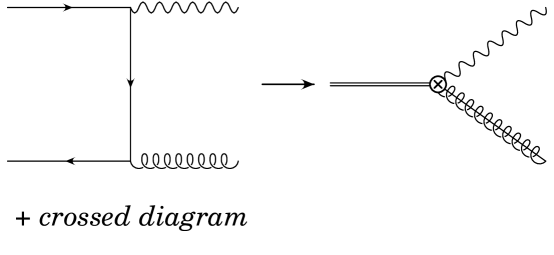
Figure 1: Matching the decay amplitude for $b\bar{b}\to\gamma+g$ in QCD and SCET. Collinear gluons are represented by a spring with a line through it.

The amplitude for a color-octet ${}^{1}S_{0}$ $b\bar{b}$ pair to decay into a photon and a collinear gluon is simply given by the Feynman rule for the color-octet ${}^{1}S_{0}$ operator in Eq. (29)

$$\Gamma^{(8,{}^{1}S_{0})}_{\alpha\mu}(M)\Big{(}\epsilon^{\alpha}_{\perp}-\frac{q^{\alpha}_{\perp}}{{\bar{n}}\cdot q}{\bar{n}}\cdot\epsilon\Big{)}\eta^{\dagger}_{-{\bf p}}T^{A}\xi_{\bf p}\,,$$ (30)

where $\eta$ and $\xi$ are two component spinors, and momentum conservation sets ${\bar{n}}\cdot q=M$. The tree level QCD expression for this amplitude expanded to order $\lambda$ is

$$2g_{s}ee_{b}\epsilon_{\alpha\mu}^{\perp}\Big{(}\epsilon_{\perp}^{\alpha}-\frac{q_{\perp}^{\alpha}}{{\bar{n}}\cdot q}{\bar{n}}\cdot\epsilon\Big{)}\eta^{\dagger}_{-{\bf p}}T^{A}\xi_{\bf p}\,,$$ (31)

where $\epsilon^{\alpha\mu}_{\perp}=\epsilon^{\alpha\mu\rho\beta}\bar{n}_{\rho}v_{\beta}$. Note there is no $\lambda^{0}$ piece. Setting the two expressions equal to each other we obtain

$$\Gamma^{(8,{}^{1}S_{0})}_{\alpha\mu}(M)=2g_{s}ee_{b}\epsilon_{\alpha\mu}^{\perp}\,.$$ (32)

The color-octet ${}^{3}P_{J}$ operator is also order $\lambda$. We give that operator and the matching coefficient in Appendix A. At order $\lambda$ these are the only two possible operators that can be constructed.

Next we construct the color-singlet ${}^{3}S_{1}$ operator at the endpoint. A $b\bar{b}$ pair in a color-singlet ${}^{3}S_{1}$ configuration decays into a photon and a collinear jet of gluons that must be colorless. The only way to construct such an operator is to include two of the $B_{\perp}$ fields in a colorless configuration. The only operator that can be constructed such that it is collinear- and usoft-gauge invariant is

$${\cal O}(1,{}^{3}S_{1})=\chi^{\dagger}_{-{\bf p}}\Lambda\cdot\mbox{\boldmath$\sigma$}^{\delta}\psi_{\bf p}{\rm Tr}\big{\{}B^{\alpha}_{\perp}\,\Gamma^{(1,{}^{3}S_{1})}_{\alpha\beta\delta\mu}(\bar{\cal P},\bar{\cal P}^{\dagger})\,B^{\beta}_{\perp}\big{\}}\,,$$ (33)

where $\bar{\cal P}^{\dagger}$ operates on the fields to the left, and $\Lambda$ boosts from the $\Upsilon$ rest frame to a frame where the $\Upsilon$ has arbitrary four-momentum bc . This operator is ${\cal O}(\lambda^{2})$ in the power counting. Once again momentum conservation forces the total momentum of the jet to be $M$, so that $B^{\alpha}_{\perp}(\bar{\cal P}+\bar{\cal P}^{\dagger})B^{\beta}_{\perp}=-MB^{\alpha}_{\perp}B^{\beta}_{\perp}$. Introducing ${\cal P}_{-}=\bar{\cal P}-\bar{\cal P}^{\dagger}$, Eq. (33) can be simplified to

$${\cal O}(1,{}^{3}S_{1})=\chi^{\dagger}_{-{\bf p}}\Lambda\cdot\mbox{\boldmath$\sigma$}^{\delta}\psi_{\bf p}{\rm Tr}\big{\{}B^{\alpha}_{\perp}\,\Gamma^{(1,{}^{3}S_{1})}_{\alpha\beta\delta\mu}(M,{\cal P}_{-})\,B^{\beta}_{\perp}\big{\}}\,.$$ (34)

The tree matching is shown in Fig. 2.

Figure 2: Matching the decay amplitude for $b\bar{b}\to\gamma+gg$ in QCD and SCET.

We obtain

$$\Gamma^{(1,{}^{3}S_{1})}_{\alpha\beta\delta\mu}(M,{\bar{n}}\cdot q_{-}) = \frac{4g_{s}^{2}ee_{b}}{3M}g_{\alpha\beta}^{\perp}\Big{[}g_{\mu\delta}+\frac{1}{2}n_{\delta}n_{\mu}\Big{]}$$ (35)

$$= \frac{4g_{s}^{2}ee_{b}}{3M}g_{\alpha\beta}^{\perp}g_{\mu\delta}\,,$$

where $g_{\perp}^{\mu\nu}=g^{\mu\nu}-(n^{\mu}\bar{n}^{\nu}+n^{\nu}\bar{n}^{\mu})/2$, ${\bar{n}}\cdot q_{-}={\bar{n}}\cdot q-{\bar{n}}\cdot q^{\prime}$, and the last line holds if the photon is transverse.

IV Factorization in Inclusive $\Upsilon\to X\gamma$

Next we show that in the endpoint region the inclusive $\Upsilon\to X\gamma$ decay rate can be factored into a hard coefficient, a collinear jet function, and a usoft function. We then perform an OPE by integrating out collinear modes at the scale $\mu_{c}\approx M\sqrt{1-z}\gg\Lambda_{\rm QCD}$, and match onto a usoft operator convoluted with a matching function. The usoft operator is nonlocal along one lightcone direction, and, as pointed out by Rothstein and Wise in Ref. Rothstein:1997ac , can be calculated for the color-singlet contribution.

The factorization proof for $\Upsilon\to X\gamma$ is similar to that of $b\to X_{s}\gamma$, and we follow Refs. Bauer:2001yt ; Bauer:2002nz . Using the optical theorem the inclusive photon energy spectrum can be written as

$$\frac{d\Gamma}{dz}=z\frac{M}{16\pi^{2}}{\rm Im}T(z)\,,$$ (36)

where the forward scattering amplitude $T(z)$ is

$$T(z)=-i\int d^{4}xe^{-iq\cdot x}\langle\Upsilon|TJ^{\dagger}_{\mu}(x)J_{\nu}(0)|\Upsilon\rangle g^{\mu\nu}_{\perp}\,.$$ (37)

The $\Upsilon$ states are relativistically normalized, and the $T$ indicates time ordering. We will show that in the endpoint region, at leading order in the SCET power counting the decay rate can be expressed in a factored form to all orders in $\alpha_{s}$

$$\frac{d\Gamma}{dz}=\sum_{\omega}H(M,\omega,\mu)\int dk^{+}S(k^{+},\mu)\;{\rm Im}\,J_{\omega}(k^{+}+M(1-z),\mu)\,.$$ (38)

The first step is to match the QCD current $J_{\mu}$ in Eq. (37) onto SCET operators. The leading order in $\lambda$ operators are the color-octet ${}^{1}S_{0}$ and ${}^{3}P_{J}$ operators. At one order higher in $\lambda$ we match onto the color-singlet operator, Eq. (33). We will show in this section how the color-singlet contribution factorizes, and leave the color-octet contribution for Appendix B.

Matching the current to leading order in $\lambda$ we obtain

$$J_{\mu}=\sum_{\omega}e^{-i(Mv+\bar{\cal P}\frac{n}{2})\cdot x}i\Gamma^{(1,{}^{3}S_{1})}_{\alpha\beta\delta\mu}(\omega)\,\tilde{J}^{\delta\alpha\beta}_{(1,{}^{3}S_{1})}(\omega)\,,$$ (39)

where the effective current is

$$\tilde{J}^{\delta\alpha\beta}_{(1,{}^{3}S_{1})}(\omega)=\chi^{\dagger}_{-{\bf p}}\Lambda\cdot\mbox{\boldmath$\sigma$}^{\delta}\psi_{\bf p}{\rm Tr}\big{\{}B^{\alpha}_{\perp}\,\delta_{\omega,{\cal P}_{-}}\,B^{\beta}_{\perp}\big{\}},$$ (40)

and $\Gamma^{(1,{}^{3}S_{1})}_{\alpha\beta\delta\mu}(\omega)$ is given in Eq. (35). Note momentum conservation forces $\bar{\cal P}\tilde{J}(\omega)=-M\tilde{J}(\omega)$, so we can replace $\bar{\cal P}$ by $-M$ in the phase factor. Substituting Eq. (39) into Eq. (37) gives

$$T(z)=\sum_{\omega,\omega^{\prime}}H_{\delta\delta^{\prime}\alpha\alpha^{\prime}\beta\beta^{\prime}}(\omega,\omega^{\prime})T^{\delta\delta^{\prime}\alpha\alpha^{\prime}\beta\beta^{\prime}}_{\rm eff}(\omega,\omega^{\prime},z,\mu)\,,$$ (41)

where

$$T^{\delta\delta^{\prime}\alpha\alpha^{\prime}\beta\beta^{\prime}}_{\rm eff}(\omega,\omega^{\prime},z,\mu)=-i\int d^{4}xe^{i(M\frac{{\bar{n}}}{2}-q)\cdot x}\langle\Upsilon|T\tilde{J}^{\delta\alpha\beta\dagger}_{(1,{}^{3}S_{1})}(\omega,x)\tilde{J}^{\delta^{\prime}\alpha^{\prime}\beta^{\prime}}_{(1,{}^{3}S_{1})}(\omega^{\prime},0)|\Upsilon\rangle\,,$$ (42)

and to leading order in $\alpha_{s}(M)$ we obtain

$$H_{\delta\delta^{\prime}\alpha\alpha^{\prime}\beta\beta^{\prime}}(\omega,\omega^{\prime})=-\left(\frac{4g_{s}^{2}ee_{b}}{3M}\right)^{2}g^{\perp}_{\alpha\beta}g^{\perp}_{\alpha^{\prime}\beta^{\prime}}g^{\perp}_{\delta\delta^{\prime}}.$$ (43)

The usoft gluons in $T^{\rm eff}$ can be decoupled from the collinear fields as explained in Ref. Bauer:2001yt by making the field redefinition

$$A^{\mu}_{n,q}=YA^{(0)\mu}_{n,q}Y^{\dagger}\hskip 14.22636pt\to\hskip 14.22636ptW=YW^{(0)}Y^{\dagger}\,,$$ (44)

where the first identity implies the second. The fields with the superscript $(0)$ do not interact with usoft physics. In the color-singlet contribution all usoft Wilson lines $Y$ cancel due to the identity $Y^{\dagger}Y=1$. Furthermore the $\Upsilon$ state contains no collinear quanta. Thus we can separate the collinear physics from the usoft physics and write the effective forward scattering amplitude as

$$T^{\delta\delta^{\prime}\alpha\alpha^{\prime}\beta\beta^{\prime}}_{\rm eff}(\omega,\omega^{\prime},z,\mu) = -i\int d^{4}xe^{\frac{i}{2}M(1-z){\bar{n}}\cdot x}\langle\Upsilon|T\big{[}\psi^{\dagger}_{\bf p}\Lambda\cdot\mbox{\boldmath$\sigma$}^{\delta}\chi_{-{\bf p}}\big{]}(x)\big{[}\chi^{\dagger}_{-{\bf p}^{\prime}}\Lambda\cdot\mbox{\boldmath$\sigma$}^{\delta^{\prime}}\psi_{{\bf p}^{\prime}}\big{]}(0)|\Upsilon\rangle$$ (45)

$$\times\langle 0|T\,{\rm Tr}\big{[}B^{(0)\alpha}_{\perp}\delta_{\omega,{\cal P}_{-}}B^{(0)\beta}_{\perp}\big{]}(x){\rm Tr}\big{[}B^{(0)\alpha^{\prime}}_{\perp}\delta_{\omega^{\prime},{\cal P}_{-}}B^{(0)\beta^{\prime}}_{\perp}\big{]}(0)|0\rangle\,,$$

where we have chosen a frame such that $q^{\mu}=\frac{M}{2}z{\bar{n}}^{\mu}$. The collinear and usoft matrix elements appearing on the left hand side of the above equation can be simplified. Using rotational invariance bc , the usoft matrix element can be written as

$$\Lambda^{\delta}_{i}\Lambda^{\delta^{\prime}}_{j}\langle\Upsilon|T\big{[}\psi^{\dagger}_{\bf p}\mbox{\boldmath$\sigma$}^{i}\chi_{-{\bf p}}\big{]}(x)\big{[}\chi^{\dagger}_{-{\bf p}^{\prime}}\mbox{\boldmath$\sigma$}^{j}\psi_{{\bf p}^{\prime}}\big{]}(0)|\Upsilon\rangle=$$

$$\qquad\frac{1}{3}\delta^{ij}\Lambda^{\delta}_{i}\Lambda^{\delta^{\prime}}_{j}\langle\Upsilon|T\big{[}\psi^{\dagger}_{\bf p}\mbox{\boldmath$\sigma$}^{k}\chi_{-{\bf p}}\big{]}(x)\big{[}\chi^{\dagger}_{-{\bf p}^{\prime}}\mbox{\boldmath$\sigma$}^{k}\psi_{{\bf p}^{\prime}}\big{]}(0)|\Upsilon\rangle\,.$$ (46)

We can then use the identity $\delta^{ij}\Lambda^{\delta}_{i}\Lambda^{\delta^{\prime}}_{j}=(v^{\delta}v^{\delta^{\prime}}-g^{\delta\delta^{\prime}})$, where $v^{\delta}$ is the four-velocity of the $\Upsilon$.

Next we define a color-singlet jet function

$$\langle 0|T\,{\rm Tr}\big{[}B^{(0)\alpha}_{\perp}\delta_{\omega,{\cal P}_{-}}B^{(0)\beta}_{\perp}\big{]}(x){\rm Tr}\big{[}B^{(0)\alpha^{\prime}}_{\perp}\delta_{\omega^{\prime},{\cal P}_{-}}B^{(0)\beta^{\prime}}_{\perp}\big{]}(0)|0\rangle \equiv$$ (47)

$$\frac{i}{2}(g^{\alpha\alpha^{\prime}}_{\perp}g^{\beta\beta^{\prime}}_{\perp}+g^{\alpha\beta^{\prime}}_{\perp}g^{\beta\alpha^{\prime}}_{\perp})\,\delta_{\omega,\omega^{\prime}}\,\int\frac{d^{4}k}{(2\pi)^{4}}e^{-ik\cdot x}J_{\omega}(k^{+},\mu)\,.$$

The jet function, $J_{\omega}(k^{+},\mu)$, is only a function of one component of the usoft momentum, $k^{+}$, which follows from the collinear Lagrangian containing only the $n\cdot\partial$ derivative Bauer:2001yt . The hard coefficient in Eq. (41) will contract with the factors in Eqs. (IV) and (47) so that the expression for the forward scattering amplitude can be written as

$$T(z)=\sum_{\omega}H(\omega,\mu)T_{\rm eff}(\omega,z,\mu)\,,$$ (48)

where

$$T_{\rm eff}(\omega,z,\mu) = \int\frac{d^{4}x}{2\pi}\int dk^{+}\delta(x^{+})\delta^{(2)}(x_{\perp})e^{\frac{i}{2}[M(1-z)-k^{+}]x^{-}}J_{\omega}(k^{+},\mu)$$ (49)

$$\qquad\times\langle\Upsilon|T\big{[}\psi^{\dagger}_{\bf p}\mbox{\boldmath$\sigma$}_{i}\chi_{-{\bf p}}\big{]}(x)\big{[}\chi^{\dagger}_{-{\bf p}^{\prime}}\mbox{\boldmath$\sigma$}_{i}\psi_{{\bf p}^{\prime}}\big{]}(0)|\Upsilon\rangle\,,$$

and the leading order hard function is

$$H(\omega,\mu)=\frac{4}{3}\left(\frac{4g_{s}^{2}ee_{b}}{3M}\right)^{2}\,.$$ (50)

Finally we define a color-singlet usoft function

$$S(\ell^{+},\mu)=\int\frac{dx^{-}}{4\pi}e^{\frac{-i}{2}\ell^{+}x^{-}}\langle\Upsilon|T\big{[}\psi^{\dagger}_{\bf p}\mbox{\boldmath$\sigma$}_{i}\chi_{-{\bf p}}\big{]}(x^{-})\big{[}\chi^{\dagger}_{-{\bf p}^{\prime}}\mbox{\boldmath$\sigma$}_{i}\psi_{{\bf p}^{\prime}}\big{]}(0)|\Upsilon\rangle\,,$$ (51)

which when substituted into Eq. (49) gives the desired factored form

$$T_{\rm eff}(\omega,z,\mu)=\int d\ell^{+}J_{\omega}[\ell^{+}+M(1-z),\mu]S(\ell^{+},\mu)\,.$$ (52)

This proves the factorization theorem Eq. (38).

V The Operator Product Expansion

As we discussed in Section III the collinear scale in $\Upsilon\to X\gamma$ decay at the endpoint is of order $\sqrt{M\Lambda_{\rm QCD}}\sim 3\,{\rm GeV}$. It is our opinion that this is large enough so that we can perform an OPE and integrate out collinear physics. However one does not have to carry out this step. Then only hard contributions are integrated out, and both the jet function and the usoft function in Eq. (38) are non-perturbative.

The OPE is carried out by expanding the jet function in powers of $\alpha_{s}(M\lambda)$, and matching onto a non-local usoft operator of the form given in Eq. (51) convoluted with a Wilson coefficient. The forward scattering amplitude will then be of the form

$$T(z)=\int d\ell^{+}S(\ell^{+},\mu){\cal H}_{J}[\ell^{+}+M(1-z),\mu]\,,$$ (53)

where the Wilson coefficient is labeled with a $J$ to remind us that it contains the hard part $H$ which is determined by matching SCET and QCD in an expansion in $\alpha_{s}(M)$. In addition it contains the perturbative expansion of the jet function in powers of $\alpha_{s}(M\sqrt{1-z})$. We now perform the OPE for the color-singlet contribution, and finally use the results of Rothstein and Wise Rothstein:1997ac to calculate the usoft function.

First we calculate the jet function, Eq. (47), to leading order. The Feynman diagram for the vacuum matrix element is shown in Fig. 3.

Figure 3: Feynman diagram for the leading order jet function.

Evaluating the diagram gives

$$\langle 0|T\,{\rm Tr}\big{[}B^{(0)\alpha}_{\perp}\delta_{\omega,{\cal P}_{-}}B^{(0)\beta}_{\perp}\big{]}(x){\rm Tr}\big{[}B^{(0)\alpha^{\prime}}_{\perp}\delta_{\omega^{\prime},{\cal P}_{-}}B^{(0)\beta^{\prime}}_{\perp}\big{]}(0)|0\rangle = -2(g^{\alpha\alpha^{\prime}}_{\perp}g^{\beta\beta^{\prime}}_{\perp}+g^{\alpha\beta^{\prime}}_{\perp}g^{\beta\alpha^{\prime}}_{\perp})$$

$$\times\int\frac{d^{4}K}{(2\pi)^{4}}\int\frac{d^{4}k}{(2\pi)^{4}}\frac{\delta_{\omega,{\bar{n}}\cdot q}\,\delta_{\omega,\omega^{\prime}}\,e^{-iK\cdot x}}{[(M+{\bar{n}}\cdot q)(K^{+}+k^{+})+q^{2}_{\perp}+i\delta][(M-{\bar{n}}\cdot q)(K^{+}-k^{+})+q^{2}_{\perp}+i\delta]}\,,$$

where we have used momentum conservation to set ${\bar{n}}\cdot q_{1}+{\bar{n}}\cdot q_{2}=M$, and $q^{\mu}_{1\perp}+q^{\mu}_{2\perp}=0$, and we let ${\bar{n}}\cdot q={\bar{n}}\cdot q_{1}-{\bar{n}}\cdot q_{2}$ and $q^{\mu}_{\perp}=q^{\mu}_{1\perp}-q^{\mu}_{2\perp}$. In addition $K$ is the sum of residual momenta and $k$ is the difference of residual momenta. In SCET there are always implicit sums over label momenta that come with collinear fields. This turns the integrals over residual momenta into integrals over the full momenta. There also is an implicit delta function which conserves label momenta. This delta function enforces the above momentum relations (see Ref. Bauer:2001ct for details). We get

$$\sum_{{\bar{n}}\cdot q}\sum_{q_{\perp}}\int\frac{d^{4}k}{(2\pi)^{4}}\to\frac{1}{2}\int\frac{dk^{+}}{2\pi}\int\frac{d{\bar{n}}\cdot q}{2\pi}\int\frac{d^{2}q_{\perp}}{(2\pi)^{2}}\,.$$ (55)

Once we make this replacement, the loop integral over the relative momentum in Eq. (V) can be performed giving

$$\langle 0|T\,{\rm Tr}\big{[}B^{(0)\alpha}_{\perp}\delta_{\omega,\bar{\cal P}}B^{(0)\beta}_{\perp}\big{]}(x){\rm Tr}\big{[}B^{(0)\alpha^{\prime}}_{\perp}\delta_{\omega^{\prime},\bar{\cal P}}B^{(0)\beta^{\prime}}_{\perp}\big{]}(0)|0\rangle = \frac{i}{2}(g^{\alpha\alpha^{\prime}}_{\perp}g^{\beta\beta^{\prime}}_{\perp}+g^{\alpha\beta^{\prime}}_{\perp}g^{\beta\alpha^{\prime}}_{\perp})\,\delta_{\omega,\omega^{\prime}}$$ (56)

$$\times\int\frac{d^{4}K}{(2\pi)^{4}}e^{-iK\cdot x}\,\frac{\Gamma(\epsilon)}{8\pi^{2}}\left(4\pi\frac{\mu^{2}}{-M^{2}-i\delta}\right)^{\epsilon}\int^{1}_{-1}d\xi\,\frac{1}{[(K^{+}/M)(1-\xi^{2})]^{\epsilon}}\,\delta_{\omega,M\xi}\,.$$

By comparing the above result to Eq. (47) it is straightforward to determine the jet function,

$$J_{\omega}(k^{+},\mu)=\frac{\Gamma(\epsilon)}{8\pi^{2}}\left(4\pi\frac{\mu^{2}}{-M^{2}-i\delta}\right)^{\epsilon}\int^{1}_{-1}d\xi\,\frac{1}{[(k^{+}/M)(1-\xi^{2})]^{\epsilon}}\,\delta_{\omega,M\xi}\,.$$ (57)

The decay rate is given by the imaginary part of the forward scattering amplitude. Taking the imaginary part of the jet function we obtain

$${\rm Im}J_{\omega}(k^{+},\mu)=\frac{1}{8\pi}\Theta(k^{+})\int^{1}_{-1}d\xi\,\delta_{\omega,M\xi}\,.$$ (58)

Substituting the above equation and the hard coefficient $H(\omega,\mu)$ into the imaginary part of the forward scattering amplitude in Eq. (48), and summing over $\omega$ gives

$${\rm Im}T(z) = \frac{2M}{M^{2}}\int d\ell^{+}\,S(\ell^{+},\mu)\,\Theta[\ell^{+}+M(1-z)]\,\frac{1}{8\pi}\int_{-1}^{1}d\xi\,H(M\xi,\mu)$$ (59)

$$= \frac{2M}{M^{2}}\int d\ell^{+}\,S(\ell^{+},\mu)\,\Theta[\ell^{+}+M(1-z)]\,\frac{16\pi}{3}\bigg{(}\frac{4\alpha_{s}(M)ee_{b}}{3M}\bigg{)}^{2}\,,$$

where the $2M/M^{2}$ accounts for the non-relativistic normalization of the $\Upsilon$ state in the usoft function. The second line is obtained by using the tree level hard coefficient Eq. (50). The integral over $\xi$ then gives only a numerical factor of two above. However, we will show in the next section that once logarithms are summed the hard coefficient depends on $\xi$ and the integral is no longer trivial. Eq. (59) is precisely in the form given in Eq. (53), and it is straightforward to read off the ${\cal H}_{J}$.

For the final step we first note that the usoft function may formally be written as

$$S(\ell^{+},\mu)=\langle\Upsilon|\psi^{\dagger}_{\bf p}\mbox{\boldmath$\sigma$}_{i}\chi_{-{\bf p}}\delta(in\cdot\partial-\ell^{+})\chi^{\dagger}_{-{\bf p}^{\prime}}\mbox{\boldmath$\sigma$}_{i}\psi_{{\bf p}^{\prime}}|\Upsilon\rangle\,.$$ (60)

It is then possible to do the integral over $\ell^{+}$ in Eq. (59), giving

$${\rm Im}T(z)=\langle\Upsilon|\psi^{\dagger}_{\bf p}\mbox{\boldmath$\sigma$}_{i}\chi_{-{\bf p}}\Theta[in\cdot\partial+M(1-z)]\chi^{\dagger}_{-{\bf p}^{\prime}}\mbox{\boldmath$\sigma$}_{i}\psi_{{\bf p}^{\prime}}|\Upsilon\rangle\,\frac{16\pi^{2}}{M}\bigg{(}\frac{32\alpha\alpha^{2}_{s}(M)e_{b}^{2}}{27m_{b}^{2}}\bigg{)}.$$ (61)

In Ref. Rothstein:1997ac it was shown that

$$\langle\Upsilon|\psi^{\dagger}_{\bf p}\mbox{\boldmath$\sigma$}_{i}\chi_{-{\bf p}}\Theta(in\cdot\partial+M-2E_{\gamma})\chi^{\dagger}_{-{\bf p}^{\prime}}\mbox{\boldmath$\sigma$}_{i}\psi_{{\bf p}^{\prime}}|\Upsilon\rangle =$$ (62)

$$\Theta(M_{\Upsilon}-2E_{\gamma})\langle\Upsilon|\psi^{\dagger}_{\bf p}\mbox{\boldmath$\sigma$}_{i}\chi_{-{\bf p}}\chi_{-{\bf p}^{\prime}}\mbox{\boldmath$\sigma$}_{i}\psi_{{\bf p}^{\prime}}|\Upsilon\rangle\,,$$

where the matrix element on the right hand side is a local operator, which can be determined from the $\Upsilon\to\ell^{+}\ell^{-}$ decay rate. Remembering that $z=2E_{\gamma}/M$ we can substitute the above equation into Eq. (61) to obtain the final expression for the imaginary part of the forward scattering amplitude

$${\rm Im}T(z)=\Theta(M_{\Upsilon}-Mz)\,\frac{16\pi^{2}}{M}\Gamma_{0},$$ (63)

where $\Gamma_{0}$ is given in Eq. (7). Plugging the above equation into Eq. (36), gives the $z\to 1$ limit of the tree level rate, Eq. (6).

VI Summing Sudakov Logarithms

One of the powers of an effective field theory approach is the ability to sum logarithms using the renormalization group equations. If there exists a hierarchy of well separated scales in a process, then logarithms of ratios of these scales arise naturally in perturbation theory. If these terms are large enough so their product with the perturbative expansion parameter is order one, then the original expansion is no longer valid. By matching onto an effective theory, as we have done here, the large scale is removed, and replaced with a running scale $\mu$. While the matching, which determines the Wilson coefficient, is carried out at the high scale, operators are run from the matching scale to the low scale using the RGEs. This sums all large logarithms into an overall factor, and any logarithms that arise in a perturbative expansion of the effective theory are order one.

As discussed previously, near the endpoint of $\Upsilon\to X\gamma$ there arises a hierarchy of scales. As an explicit example consider the color-octet ${}^{1}S_{0}$ processes. We studied the endpoint behavior of this contribution in a previous work Bauer:2001rh . At next-to-leading order in $\alpha_{s}$ the Wilson coefficient in the $z\to 1$ limit is

$$C_{\bf 8}^{(1)}(^{1}S_{0})(z) = \frac{\alpha_{s}}{2\pi}\tilde{C}_{\bf 8}^{(0)}(^{1}S_{0})\left[-2C_{A}\left(\frac{\log(1-z)}{1-z}\right)_{+}-\left(\frac{23}{6}C_{A}-\frac{n_{f}}{3}\right)\left(\frac{1}{1-z}\right)_{+}\right],$$ (64)

where $\tilde{C}_{\bf 8}^{(0)}(^{1}S_{0})=16\alpha_{s}\alpha e_{b}^{2}\pi/M^{2}$. If this coefficient is integrated over the endpoint region ($1-v^{2}<z<1$), the first plus distribution on the right-hand side gives rise to a double logarithm, $\log^{2}v^{2}$, and the second plus distribution gives a single logarithm, $\log v^{2}$. Both of these are numerically of order $1/\alpha_{s}$. This clearly ruins the perturbative expansion. We showed in Ref.  Bauer:2001rh that these large logarithms are summed by matching onto SCET at the scale $M$ and running to the usoft scale. The is also true of the color-octet ${}^{3}P_{J}$ contribution.

For the color-singlet ${}^{3}S_{1}$ contribution we can not explicitly give the NLO contribution in the endpoint region since this has only been calculated numerically Kramer:1999bf . However, while the NLO correction to the color-singlet contribution does not change the LO prediction very much for low and intermediate values of $z$, it does change the endpoint prediction by an amount of order one. This, as we will show, is due to the presence of endpoint logarithms. However, unlike the color-octet case these endpoint logarithms are single, not double logarithms.

In Section III we matched onto the SCET color-singlet operator. This integrates out the scale $M$. We now run the color-singlet operator from the hard scale to the collinear scale, which sums all logarithms of $1-z$. Unlike the color-octet contribution the color-singlet operator does not run below the collinear scale. To run the color-singlet operator given in Eq. (34), we calculate the counterterm for the operator, then determine the anomalous dimension, and finally use this in the RGEs. The four graphs that need to be evaluated to obtain the counterterm are shown in Fig. 4.

  

  

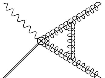
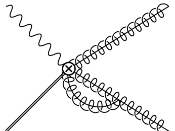
Figure 4: Diagrams needed to calculate the counterterm to the color-singlet operator.

Note that the diagrams only involve collinear gluons. All of the diagrams involving usoft gluons vanish because the color-singlet process is transparent to usoft gluons. This is clear from the previous section where we showed that usoft Wilson lines completely cancel in the color-singlet contribution. This is very different than the color-octet contribution where usoft gluons play a crucial role. The Feynman rules for the vertex operators are given in Appendix A. The result of each of the loop integrals is complicated so we do not give each individual expression. However, when all the terms are added we obtain a relatively simple result for the one-loop UV-divergent term

$${\cal A} = \frac{1}{\epsilon}\,\chi^{\dagger}_{-{\bf p}}\Lambda\cdot\mbox{\boldmath$\sigma$}^{\delta}\psi_{\bf p}\sum_{\omega}\Gamma^{(1,{}^{3}S_{1})}_{\alpha\beta\delta\mu}(M,\omega){\rm Tr}\big{\{}B^{\alpha}_{\perp}\,\delta_{\omega,{\cal P}_{-}}\,B^{\beta}_{\perp}\big{\}}$$

$$\qquad\qquad\times\frac{\alpha_{s}(\mu)C_{A}}{2\pi}\bigg{[}1+\frac{M^{2}+\omega^{2}}{M^{2}}\bigg{(}\frac{M}{M+\omega}\ln\frac{M-\omega}{2M}+\frac{M}{M-\omega}\ln\frac{M+\omega}{2M}\bigg{)}\bigg{]},$$

where we have introduced a sum over the index $\omega$. Note that the divergent contribution depends on the large momentum component of the collinear gluons. This means that the counterterm will depend on the large momentum components, as will the anomalous dimension. This divergent piece must be canceled by $Z_{3}/Z_{\cal O}-1$, where $Z_{\cal O}$ is the counterterm for the color-singlet vertex in SCET, and $Z_{3}$ is the gluon wave function counterterm

$$Z_{3}=1+\frac{\alpha_{s}}{4\pi}\frac{1}{\epsilon}\left(C_{A}\frac{5}{3}-n_{f}\frac{2}{3}\right)\,.$$ (66)

This leads to

$$Z_{\cal O}-1=\frac{1}{\epsilon}\,\frac{\alpha_{s}}{2\pi}\bigg{\{}C_{A}\bigg{[}\frac{11}{6}+\frac{M^{2}+\omega^{2}}{M^{2}}\bigg{(}\frac{M}{M+\omega}\ln\frac{M-\omega}{2M}+\frac{M}{M-\omega}\ln\frac{M+\omega}{2M}\bigg{)}\bigg{]}-\frac{n_{f}}{3}\bigg{\}}\,.$$ (67)

The anomalous dimension is obtained through the standard method, and the RGE for the color-singlet Wilson coefficient is

$$\mu\frac{d}{d\mu}\Gamma^{(1,{}^{3}S_{1})}(\mu,\omega)=\gamma(\mu,\omega)\Gamma^{(1,{}^{3}S_{1})}(\mu,\omega)\,.$$ (68)

We have made the dependence on the momentum label $\omega$ explicit to emphasize that the anomalous dimension depends on these labels. Solving the RGE gives

$$\ln\!\bigg{(}\frac{\Gamma^{(1,{}^{3}S_{1})}(\mu,\omega)}{\Gamma^{(1,{}^{3}S_{1})}(M,\omega)}\bigg{)} =$$

$$\frac{2}{\beta_{0}}\bigg{\{}C_{A}\bigg{[}\frac{11}{6}+\frac{M^{2}+\omega^{2}}{M^{2}}\bigg{(}\frac{M}{M+\omega}\ln\frac{M-\omega}{2M}+\frac{M}{M-\omega}\ln\frac{M+\omega}{2M}\bigg{)}\bigg{]}-\frac{n_{f}}{3}\bigg{\}}\ln\!\bigg{(}\frac{\alpha_{s}(\mu)}{\alpha_{s}(M)}\bigg{)},$$

where $\Gamma^{(1,{}^{3}S_{1})}(M,\omega)$ is given in Eq. (35). Logarithms of the form $\ln(\mu/M)$ have been summed into $\Gamma^{(1,{}^{3}S_{1})}(\mu,\omega)$, and any logarithms in the operator are of the form $\ln(\mu_{c}/\mu)$, where $\mu_{c}\approx M\sqrt{1-z}$ is the collinear scale. If we take $\mu\sim\mu_{c}$ logarithms in the operator will be small, and all large logarithms of the ratio $\mu_{c}/M$ will sit in the Wilson coefficient.

We can now obtain the resummed rate, by substituting the Wilson coefficient at the collinear scale $\mu=M\sqrt{1-z}$, Eq. (VI), into Eq. (59), giving

$${\rm Im}T(z) = 2M\int d\ell^{+}\,S(\ell^{+},\mu)\,\Theta[\ell^{+}+M(1-z)]\,\frac{16\pi}{3}\bigg{(}\frac{4\alpha_{s}(M)ee_{b}}{3M^{2}}\bigg{)}^{2}$$

$$\times\int_{0}^{1}d\eta\bigg{[}\frac{\alpha_{s}(M\sqrt{1-z})}{\alpha_{s}(M)}\bigg{]}^{2\gamma(\eta)},$$

where

$$\gamma(\eta)\equiv\frac{2}{\beta_{0}}\bigg{\{}C_{A}\bigg{[}\frac{11}{6}+\big{(}\eta^{2}+(1-\eta)^{2}\big{)}\bigg{(}\frac{1}{1-\eta}\ln\eta+\frac{1}{\eta}\ln(1-\eta)\bigg{)}\bigg{]}-\frac{n_{f}}{3}\bigg{\}}.$$ (71)

We have substituted $\xi=2\eta-1$. As in the previous section, using the formal result for the usoft function, Eq. (60), and the results of Ref. Rothstein:1997ac we obtain the final expression for the imaginary part of the forward scattering amplitude including resummation

$${\rm Im}T(z)=\Theta(M_{\Upsilon}-Mz)\,\frac{16\pi^{2}}{M}\Gamma_{0}\int_{0}^{1}d\eta\bigg{[}\frac{\alpha_{s}(M\sqrt{1-z})}{\alpha_{s}(M)}\bigg{]}^{2\gamma(\eta)}\,,$$ (72)

where $\Gamma_{0}$ is given in Eq. (7). The resummed color-singlet contribution to the decay rate in the endpoint region is obtained by inserting the above equation into Eq. (36)

$$\frac{1}{\Gamma_{0}}\frac{d\Gamma_{\rm resum}}{dz}=\Theta(M_{\Upsilon}-Mz)\,z\int_{0}^{1}d\eta\bigg{[}\frac{\alpha_{s}(M\sqrt{1-z})}{\alpha_{s}(M)}\bigg{]}^{2\gamma(\eta)}.$$ (73)

Note we can expand Eq. (73) in powers of $\alpha_{s}(M)$ and obtain an analytic expression for the NLO logarithmic contribution

$$\frac{1}{\Gamma_{0}}\frac{d\Gamma}{dz}=z\bigg{\{}1+\frac{\alpha_{s}(M)}{6\pi}\big{[}C_{A}(2\pi^{2}-17)+2n_{f}\big{]}\ln(1-z)\bigg{\}}\,.$$ (74)

As $z$ approaches one the ${\cal O}(\alpha_{s})$ term becomes negative and of order one, precisely the behavior observed in Ref. Kramer:1999bf for the NLO decay rate at the endpoint.

VII Phenomenology and Discussion

In this section we combine the different contributions to obtain a prediction for the photon spectrum in $\Upsilon\to X\gamma$ decay. We will marry our expression for the color-singlet spectrum in the endpoint with the leading order result by interpolating between the two

$$\frac{1}{\Gamma_{0}}\frac{d\Gamma_{\rm int}}{dz}=\bigg{(}\frac{1}{\Gamma_{0}}\frac{d\Gamma_{\rm LO}^{\rm dir}}{dz}-z\bigg{)}+\frac{1}{\Gamma_{0}}\frac{d\Gamma_{\rm resum}}{dz}\,.$$ (75)

The term in brackets vanishes as $z\to 1$, leaving only the resummed contribution in that region. Away from the endpoint the resummed contribution combines with the $-z$ to give higher order in $\alpha_{s}(M)$ corrections. This clear from Eq. (74).

Before we proceed we need the NRQCD matrix elements. The color-singlet matrix element can be related to the wavefunction at the origin, Eq. (5), which can be calculated in potential models, on the lattice, or extracted from the $\Upsilon$ leptonic decay rate,

$$\Gamma(\Upsilon\to e^{+}e^{-})=\frac{2\pi\alpha^{2}e_{b}^{2}}{3}\left[1-\frac{8}{3}\frac{\alpha_{s}(m_{b})}{\pi}-\frac{1}{3}\frac{M_{\Upsilon(nS)}-2m_{b}}{2m_{b}}\right]^{2}\frac{\langle\Upsilon|{\cal O}_{1}(^{3}S_{1})|\Upsilon\rangle}{m_{b}^{2}}.$$ (76)

The relativistic correction was first expressed in terms of $M_{\Upsilon}-2m_{b}$ by Gremm and Kapustin Gremm:1997dq . The matrix element is sensitive to the value of the $b$ quark mass. We will use $m_{b}=4.8$ GeV, and $\alpha_{s}(m_{b})=0.21$, giving $\langle\Upsilon|{\cal O}_{1}(^{3}S_{1})|\Upsilon\rangle=3.40{\rm\ GeV}^{3}$.

The color-octet matrix elements are more difficult to determine. They can, in principle, be extracted from data or calculated on the lattice (e.g., see Ref. Bodwin:2001mk ). NRQCD predicts that the color-octet matrix elements scale as $v^{4}$ compared to the color-singlet matrix element. In Ref. Petrelli:1998ge it was argued that a factor of $1/2N_{c}$ should be included in a naive estimate of the color-octet matrix elements. For now, we leave these parameters free.

For the color-octet ${}^{1}S_{0}$ and ${}^{3}P_{0}$ rates, we need a structure function Rothstein:1997ac ; Wolf:2001pm . We will use the simple model introduced in Ref. Bauer:2001rh

$$f(k^{+}) = N\left(1-\frac{k^{+}+\Lambda_{1}}{\bar{\Lambda}}\right)^{a}\,e^{(1+a)(k^{+}+\Lambda_{1})/\bar{\Lambda}}\;,$$ (77)

where $N$ is chosen so that the integral of the structure function is normalized to one. In principle the structure function can be different for the different color-octet states. But since we are ignorant of the non-perturbative structure function, we will naively use the same model for both the ${}^{1}S_{0}$ and ${}^{3}P_{0}$ configurations. For quarkonium the first moment of the structure function with respect to $k^{+}$ is

$$\Lambda_{1}=\frac{\langle\Upsilon|\sum_{{\bf p},{\bf p^{\prime}}}[\psi^{\dagger}_{\bf p^{\prime}}T^{a}\Gamma_{i}\chi_{-{\bf p^{\prime}}}]iD^{+}[\chi^{\dagger}_{-{\bf p}}T^{a}\Gamma_{i}\psi_{\bf p}]|\Upsilon\rangle}{\langle\Upsilon|\sum_{{\bf p},{\bf p^{\prime}}}[\psi^{\dagger}_{\bf p^{\prime}}T^{a}\Gamma_{i}\chi_{-{\bf p^{\prime}}}][\chi^{\dagger}_{-{\bf p}}T^{a}\Gamma_{i}\psi_{\bf p}]|\Upsilon\rangle}\,.$$ (78)

The integration limits for $k^{+}$ are from $-M$ to $M_{\Upsilon}-M$, and both $\bar{\Lambda}$ and $\Lambda_{1}$ are non-perturbative parameters related through $\bar{\Lambda}=M_{\Upsilon}-M-\Lambda_{1}$. We use the following numbers in our plots: $a=1$, $\bar{\Lambda}=480\,{\rm MeV}$, and $\Lambda_{1}=-620\,{\rm MeV}$.

In Fig. 5 we show the color-singlet rate.

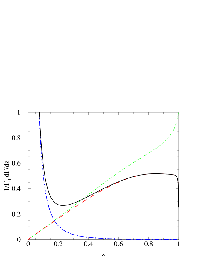
Figure 5: The color-singlet rate. The dotted curve is the tree-level direct rate. The dashed curve is the interpolated resummed direct rate. The dot-dashed curve is the fragmentation contribution, and the solid curve is the sum of the resummed rate and the fragmentation rates.

Since each contribution is proportional to the same matrix element, we can normalize the rate to $\Gamma_{0}$ in Eq. (7). The dotted curve is the tree-level direct rate, Eq. (6), the dashed is the interpolated resummed result, Eq. (75), the dot-dashed is the fragmentation contribution, Eq. (12), and the solid is the sum of the interpolated resummed and fragmentation contributions. As can be seen, the resummed rate rate turns over and decreases near the endpoint. At some point the resummed rate has a problem with the Landau pole, which can be handled in a manner described in Ref. Leibovich:2001ra ; however the Landau pole is not reached until $z\sim 0.999$, at which point the curve is in the resonance region and our results are no longer valid.

The resummed result depends on the collinear scale. In Fig. 5 the collinear scale was set to $\mu_{c}=M\sqrt{1-z}$. In Fig. 6 the solid curve again uses this choice of $\mu_{c}$.

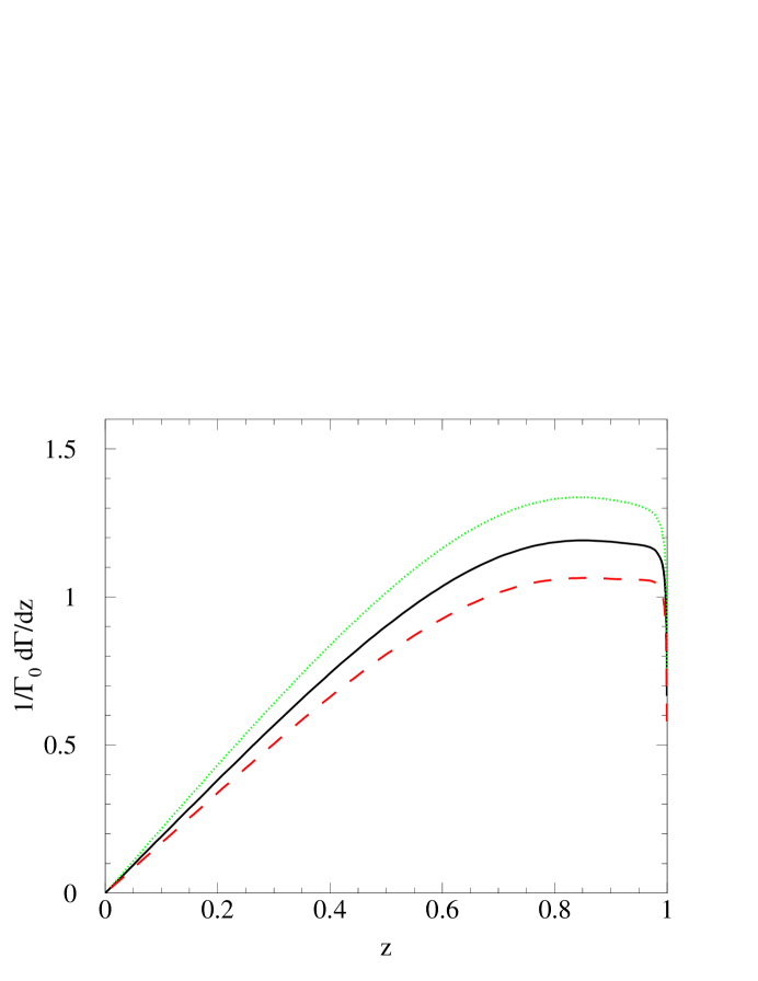
Figure 6: The resummed color-singlet rate for different choices of collinear scale $\mu_{c}$. The solid curve uses $\mu_{c}=M\sqrt{1-z}$, the dotted $\mu_{c}=M\sqrt{2(1-z)}$, and the dashed $\mu_{c}=M\sqrt{(1-z)/2}$.

The dotted is made with the collinear scale set to $\mu_{c}=M\sqrt{2(1-z)}$, and the dashed has $\mu_{c}=M\sqrt{(1-z)/2}$. The choice of scale is a higher order effect, which can only be determined by calculating higher order corrections to our results. The scale variation changes the rate by about 10%. This can be considered part of the theoretical uncertainty.

We also need to include the color-octet contributions to the decay rate, which requires knowledge of the the color-octet matrix elements. Since these are unknown at present, we first show in Fig. 7 the color-octet contributions with arbitrary choices of $\langle\Upsilon|{\cal O}_{8}(^{3}S_{1})|\Upsilon\rangle$ and

$$\langle\Upsilon|{\cal O}_{8}(^{1}S_{0})|\Upsilon\rangle+7\frac{\langle\Upsilon|{\cal O}_{8}(^{3}P_{0})|\Upsilon\rangle}{m_{b}^{2}},$$ (79)

the linear combination which occurs in both the fragmentation and the resummed rates. The solid curve is the octet ${}^{3}S_{1}$ fragmentation contribution, and the dashed curve is the octet ${}^{1}S_{0}$ and ${}^{3}P_{0}$ resummed rate convoluted with the shape function added to the octet ${}^{1}S_{0}$ and ${}^{3}P_{0}$ fragmentation rate.

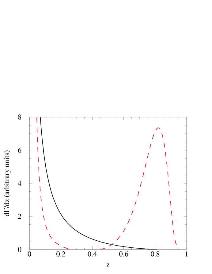
Figure 7: The color-octet rate with arbitrary choice of NRQCD matrix elements. The solid curve is the octet ${}^{3}S_{1}$ fragmentation contribution, while the dashed curve is the octet ${}^{1}S_{0}$ and ${}^{3}P_{0}$ resummed rate convoluted with the shape function and the octet ${}^{1}S_{0}$ and ${}^{3}P_{0}$ fragmentation rate.

The ${}^{3}S_{1}$ octet fragmentation rate has support at larger values of $z$ than the other fragmentation contributions at this order. However, higher order perturbative corrections to the other octet fragmentation contributions do increase the support at higher $z$ Maltoni:1999nh . The resummed octet rate produces a large peak near $z\sim 0.8$ which does not appear to be present in the data. We will therefore have to choose the combination in Eq. (79) to be small enough to agree with data.

The CLEO collaboration has measured the number of photons in inclusive $\Upsilon(1S)$ radiative decays in Ref. Nemati:1996xy . The data presented does not remove the efficiency or energy resolution and is the number of photons in the barrel region of the detector, $|\cos\theta|<0.7$. Therefore, in order to compare our theoretical prediction to the data, we first integrate over the barrel region and then convolute with the efficiency that was modeled in the CLEO paper. We did not do a bin-to-bin smearing of our prediction. Since we do not know the size of the color-octet matrix elements, we will set the ${}^{1}S_{0}$ and ${}^{3}P_{0}$ matrix elements to zero, and the ${}^{3}S_{1}$ matrix element to

$$\langle\Upsilon|{\cal O}_{8}(^{3}S_{1})|\Upsilon\rangle=v^{4}\langle\Upsilon|{\cal O}_{1}(^{3}S_{1})|\Upsilon\rangle,$$ (80)

where we set $v^{2}=0.08$.

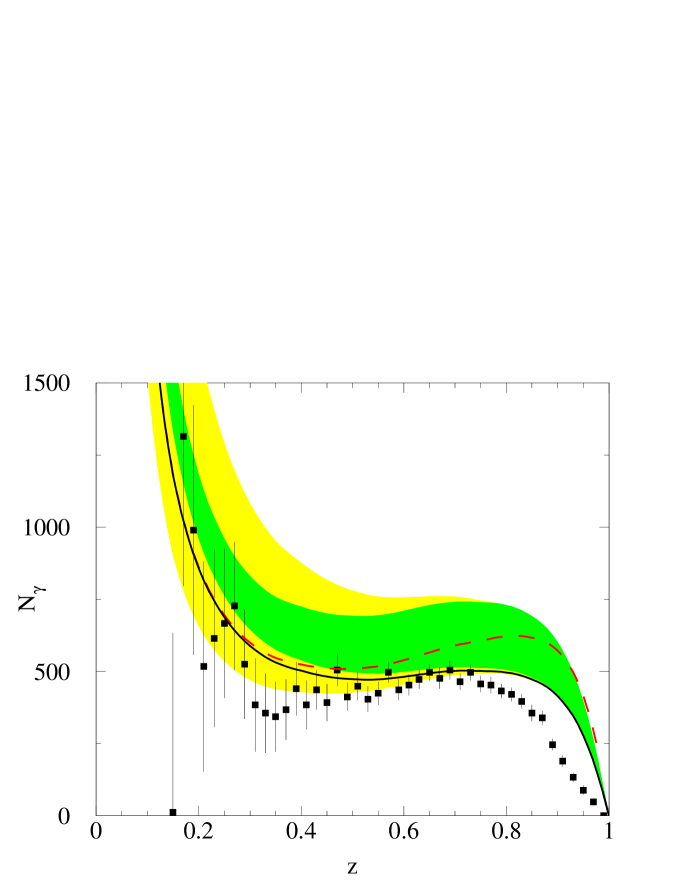
Figure 8: The inclusive radiative $\Upsilon$ photon spectrum, compared with data from CLEO Nemati:1996xy . The error bars on the data are statistical only. The theoretical prediction, shown by the solid curve, includes the color-singlet interpolated resummed and fragmentation contribution and the color-octet ${}^{3}S_{1}$ fragmentation contribution, with $\alpha_{s}$ set to the value extracted in Nemati:1996xy . The other color-octet matrix elements are set to zero. The dashed line is the direct tree-level and fragmentation result, with the same choice of $\alpha_{s}$. The theoretical prediction using the PDG value for $\alpha_{s}$, shown by the shaded bands, includes the color-singlet interpolated resummed plus fragmentation contribution and the color-octet ${}^{3}S_{1}$ fragmentation contribution. The inner band is obtained by varying $m_{b}$, $\alpha_{s}$, and the collinear scale, while the outer band includes variation of the fragmentation function, as described in the paper.

In Fig. 8 we compare our prediction to the data. The error bars on the data are statistical only. The dashed line is the direct tree-level and fragmentation result, and the solid curve is the sum of the interpolated resummed result and the fragmentation result. For these two curves we used the value of $\alpha_{s}$ extracted by CLEO from these data, $\alpha_{s}(M_{\Upsilon})=0.163$, which corresponds to $\alpha_{s}(M_{Z})=0.110$ Nemati:1996xy . While not a perfect fit, the shape of the resummed result is closer to the data than the tree-level curve. We also show in this plot the interpolated resummed and fragmentation result, using the PDG value of $\alpha_{s}(M_{Z})$, including theoretical uncertainties, denoted by the shaded region. To obtain the darker band, we first varied the choice of $m_{b}$ between $4.7{\rm\ GeV}<m_{b}<4.9{\rm\ GeV}$ and the value of $\alpha_{s}$ within the errors given in the PDG, $\alpha_{s}(M_{Z})=0.1172\pm 0.002$ Hagiwara:pw . Varying $m_{b}$ and $\alpha_{s}$ modifies the extraction of the color-singlet matrix element in Eq. (76) from $3.31{\rm\ GeV}^{3}$ to $3.56{\rm\ GeV}^{3}$. We also varied the collinear scale, $\mu_{c}$ as we did in Fig. 6 from $M\sqrt{(1-z)/2}<\mu_{c}<M\sqrt{2(1-z)}$. Finally, the lighter band also includes the variation, within the errors, of the parameters for the quark to photon fragmentation function, Eq. (17), that was extracted by ALEPH Buskulic:1995au . The low $z$ prediction is dominated by the quark to photon fragmentation coming from the color-octet ${}^{3}S_{1}$ channel. We did not assign any error to the color-octet ${}^{3}S_{1}$ matrix element. Since it is unknown, there is a very large uncertainty in the lower part of the prediction that we decided not to show. We also do not include in our error estimate contributions from higher order SCET operators, which are generically suppressed by a least a power of $\lambda/M\sim\sqrt{1-z}$. Note that the color-octet ${}^{1}S_{0}$ and ${}^{3}P_{0}$ contribution increases the theoretical prediction at the upper endpoint, as shown in Fig. 7. It is thus clear the data favors a very small value for the linear combination Eq. (79). This is why we set these matrix elements to zero in our analysis. If we used small negative values for these matrix elements we would fit the shape in the endpoint region a bit better.

As mentioned earlier, the NLO calculation of the photon spectrum was previously calculated numerically in Ref. Kramer:1999bf . The $\alpha_{s}$ correction is small for low and intermediate values of $z$, but becomes larger above $z\approx 0.8$ until it is of order one above $z\approx 0.9$. Much of the difference between the LO and NLO piece in the endpoint is due to a $\alpha_{s}\log(1-z)$ term. However, some of the difference is due to the non-logarithmic contributions. Here we resummed logarithms of the form $\alpha_{s}\log(1-z)$ so our result includes the logarithmic piece of the NLO contribution. However, we do not incorporate any of the non-logarithmic NLO corrections. This would be done by matching onto SCET at NLO. Since some of the difference between the shape of the LO and NLO contribution at the endpoint is due to these terms, a NLO matching may give a better fit to data in the endpoint region.

The logarithms in the color-singlet rate have previously been studied in Refs. Photiadis:1985hn ; Hautmann:2001yz . In Ref. Photiadis:1985hn collinear logarithms were summed including mixing with quarks. Since we neglected mixing with quark operators (see footnote 4) we compare to the expression obtained in Ref. Photiadis:1985hn by setting the quark contribution zero. When we do that we find that the results are in agreement. In Ref. Hautmann:2001yz it was argued that all logarithms cancel in the color-singlet rate, which is not what we found. However, the analysis of Ref. Hautmann:2001yz was based on the eikonal approximation, which is equivalent to including only usoft gluon modes. It did not include purely collinear modes. We do agree with the statement in Ref. Hautmann:2001yz that all logarithms due to usoft gluons cancel in the rate. This is clear in Section IV where we found that at leading order in $\lambda$ the usoft Wilson lines cancel in the usoft function. Equivalently we saw this cancellation in Section VI where we found that here are no diagrams renormalizing the color-singlet operator involving usoft gluons. However, there are logarithms due to collinear gluons. Note that at higher order in $\lambda$, there would be diagrams with usoft gluons renomalizing the operator. This would correspond to logarithms in the derivative of the rate, whose existence was pointed out in Ref. Hautmann:2001yz .

In Ref. Field:cy a model is introduced based on the idea that the outgoing gluons shower to produce a jet of particles with a non-zero invariant mass. Specifically in this model gluons are given a mass of order $m_{g}\sim 1{\rm\ GeV}$, which is an estimate based on a Monte Carlo calculation of the invariant mass of the final state jet. It is found that this approach gives a very good fit to the data Field:2001iu . If, as was discussed at the beginning of Section V, we treat the collinear scale $M\sqrt{1-z}$ as non-perturbative, we would also be forced to introduce a model for the jet and usoft functions (since they would be non-perturbative). This approach would then be equivalent to the approach in Refs. Field:cy ; Field:2001iu , if we used as a model for the jet function the LO calculation carried out in Section V including a gluon mass of order $m_{g}\sim 1{\rm\ GeV}$.

VIII conclusion

The photon energy spectrum in $\Upsilon\to X\gamma$ decay proves to be far richer than the simple leading order prediction based upon the color-singlet model. As was first pointed out in Ref. Catani:1995iz , at low photon energies it is crucial to include fragmentation contributions. In addition it has long been known that at high photon energies usoft gluon effects must be incorporated. In Ref. Field:cy a model was introduced to accomplish this, however, the result is no longer a prediction of QCD alone. In this paper we systematically treat the endpoint region in the soft-collinear effective theory. Because SCET is constructed to reproduce QCD in the endpoint region the results of our calculation are model independent predictions of QCD.

Specifically we have determined the behavior of the color-singlet contribution at the endpoint. This calculation consists of matching onto a color-singlet operator in SCET, and running the operator from the matching scale to the collinear scale. The first step integrates out the hard scale set by the $\Upsilon$ mass, and the second step sums logarithms of the ratio of the hard and collinear scales. Our result for the logarithms agrees with Ref. Photiadis:1985hn . Finally we obtain the decay rate by performing an OPE and matching onto a color-singlet shape function. As pointed out by Rothstein and Wise Rothstein:1997ac this shape function can be calculated.

We combine the color-singlet contribution with the color-octet contribution calculated in Ref. Bauer:2001rh to obtain a complete theoretical prediction for the photon spectrum at the endpoint. Furthermore we combine our result with an NRQCD calculation that includes the fragmentation contribution at low photon energy to obtain a theoretical prediction for the entire photon spectrum. We compare our calculation to data taken by the CLEO collaboration Nemati:1996xy . Overall there is good agreement with the data. Moreover the results at the endpoint are now in much better agreement with data than they were previously with the leading order NRQCD prediction. However there is still a discrepancy between data and theory, and in the size and shape of the spectrum. This discrepancy might be corrected by including contributions that are higher order in strong coupling $\alpha_{s}$ and the SCET power counting $\lambda$.

Appendix A SCET operators and Feynman rules

The most general ${}^{3}P_{J}$ operator is given by

$$\chi^{\dagger}_{-{\bf p}}\Gamma_{\alpha\mu\sigma\delta}(\bar{\cal P})B^{\alpha}_{\perp}\Lambda\cdot\widehat{{\bf p}}^{\sigma}\Lambda\cdot\mbox{\boldmath$\sigma$}^{\delta}\psi_{\bf p}\,,$$ (81)

where the tree level Feynman rule for this operator is

$$\Gamma_{\alpha\mu\sigma\delta}(\omega)\Big{(}\epsilon^{\perp}_{\alpha}-\frac{q^{\perp}_{\alpha}}{{\bar{n}}\cdot q}{\bar{n}}\cdot\epsilon\Big{)}\Lambda\cdot\widehat{{\bf p}}^{\sigma}\eta^{\dagger}_{-{\bf p}}\Lambda\cdot\mbox{\boldmath$\sigma$}^{\delta}T^{A}\xi_{\bf p}\,,$$ (82)

and $\widehat{{\bf p}}=p/M$. To match we expand the tree level QCD amplitude to leading order in $\lambda$:

$$4g_{s}ee_{b}(g^{\perp}_{\alpha\delta}g^{\perp}_{\mu\sigma}+g^{\perp}_{\alpha\sigma}g^{\perp}_{\mu\delta}+g^{\perp}_{\alpha\sigma}n^{\delta}{\bar{n}}^{\mu}-g^{\perp}_{\alpha\mu}n^{\delta}n^{\sigma})\Big{(}\epsilon^{\perp}_{\alpha}-\frac{q^{\perp}_{\alpha}}{{\bar{n}}\cdot q}{\bar{n}}\cdot\epsilon\Big{)}\Lambda\cdot\widehat{{\bf p}}^{\sigma}\eta^{\dagger}_{-{\bf p}}\Lambda\cdot\mbox{\boldmath$\sigma$}^{\delta}T^{A}\xi_{\bf p}\,.$$ (83)

If we take the photon to be real (i.e. to only have $\perp$ polarization) then the ${\bar{n}}^{\mu}$ term vanishes and the matching coefficient is

$$\Gamma^{\alpha\mu\sigma\delta}(M)=4g_{s}ee_{b}(g^{\perp}_{\alpha\delta}g^{\perp}_{\mu\sigma}+g^{\perp}_{\alpha\sigma}g^{\perp}_{\mu\delta}-g^{\perp}_{\alpha\mu}n^{\delta}n^{\sigma})\,.$$ (84)

Next we give Feynman rules for the color-singlet operator at order $g^{2}_{s}$, and order $g_{s}^{3}$ To obtain the $g^{2}_{s}$ Feynman rule we first expand Eq. (33) to order $g_{s}^{2}$

$${\cal O}(1,{}^{3}S_{1}) = \sum_{p}\chi^{\dagger}_{-{\bf p}}\Lambda\cdot\mbox{\boldmath$\sigma$}_{\delta}\psi_{\bf p}{\bar{n}}\cdot q{\bar{n}}\cdot q^{\prime}\Gamma^{\alpha\beta\delta\mu}({\bar{n}}\cdot q,{\bar{n}}\cdot q^{\prime})$$ (85)

$${\rm Tr}\Big{\{}\Big{(}\frac{{\bar{n}}\cdot A_{n,q}}{{\bar{n}}\cdot q}q^{\alpha}_{\perp}-(A^{\alpha}_{n,q})_{\perp}\Big{)}\Big{(}\frac{{\bar{n}}\cdot A_{n,q^{\prime}}}{{\bar{n}}\cdot q^{\prime}}q^{\prime\beta}_{\perp}-(A^{\beta}_{n,q^{\prime}})_{\perp}\Big{)}\Big{\}}\,,$$

where $\Gamma^{\alpha\beta\delta\mu}$ is given in Eq. (35), which gives the following tree-level Feynman rule:

$${\cal A}(1,{}^{3}S_{1}) = \eta^{\dagger}_{-{\bf p}}\Lambda\cdot\mbox{\boldmath$\sigma$}_{\delta}\xi_{\bf p}\Gamma^{\alpha\beta\delta\mu}({\bar{n}}\cdot q,{\bar{n}}\cdot q^{\prime})$$ (86)

$$\Big{(}\frac{{\bar{n}}\cdot\epsilon_{n,q}}{{\bar{n}}\cdot q}q^{\alpha}_{\perp}-(\epsilon^{\alpha}_{n,q})_{\perp}\Big{)}\Big{(}\frac{{\bar{n}}\cdot\epsilon_{n,q^{\prime}}}{{\bar{n}}\cdot q^{\prime}}q^{\prime\beta}_{\perp}-(\epsilon^{\beta}_{n,q^{\prime}})_{\perp}\Big{)}\delta^{ab}\,.$$

Expanding Eq. (33) to order $g_{s}^{3}$ gives

$${\cal O}_{g}(1,{}^{3}S_{1}) = ig_{s}\eta^{\dagger}_{-{\bf p}}\Lambda\cdot\mbox{\boldmath$\sigma$}_{\delta}\xi_{\bf p}\Gamma^{\alpha\beta\delta\mu}({\bar{n}}\cdot q,{\bar{n}}\cdot q^{\prime})$$ (87)

$$\Big{[}-q^{\prime}_{\perp}\cdot(A^{a}_{n,q})_{\perp}+q_{\perp}\cdot q^{\prime\prime}_{\perp}\frac{{\bar{n}}\cdot A_{n,q}}{{\bar{n}}\cdot q}\Big{]}\frac{{\bar{n}}\cdot A_{n,q^{\prime}}}{{\bar{n}}\cdot q^{\prime}}\frac{{\bar{n}}\cdot A_{n,q^{\prime\prime}}}{{\bar{n}}\cdot(q^{\prime}+q^{\prime\prime})}\,,$$

which gives the Feynman rule

$$i{\cal A}_{g}(1,^{3}S_{1}) = -\frac{8ee_{b}g_{s}^{3}}{3M}\eta^{\dagger}_{-{\bf p}}\Lambda\cdot\mbox{\boldmath$\sigma$}^{\mu}\xi_{\bf p}f^{abc}\left\{\frac{{\bar{n}}^{\alpha}{\bar{n}}^{\beta}}{{\bar{n}}\cdot(g_{1}+g_{2})}\left(\frac{g_{2\perp}^{\gamma}}{{\bar{n}}\cdot g_{2}}-\frac{g_{1\perp}^{\gamma}}{{\bar{n}}\cdot g_{1}}\right)\right.$$ (88)

$$+\frac{{\bar{n}}^{\beta}{\bar{n}}^{\gamma}}{{\bar{n}}\cdot(g_{2}+g_{3})}\left(\frac{g_{3\perp}^{\alpha}}{{\bar{n}}\cdot g_{3}}-\frac{g_{2\perp}^{\alpha}}{{\bar{n}}\cdot g_{2}}\right)+\frac{{\bar{n}}^{\gamma}{\bar{n}}^{\alpha}}{{\bar{n}}\cdot(g_{3}+g_{1})}\left(\frac{g_{1\perp}^{\gamma}}{{\bar{n}}\cdot g_{1}}-\frac{g_{3\perp}^{\gamma}}{{\bar{n}}\cdot g_{3}}\right)$$

$$+{\bar{n}}^{\alpha}{\bar{n}}^{\beta}{\bar{n}}^{\gamma}\left[\frac{g_{1\perp}\cdot g_{2\perp}}{{\bar{n}}\cdot g_{3}}\left(\frac{1}{{\bar{n}}\cdot g_{2}{\bar{n}}\cdot(g_{1}+g_{3})}-\frac{1}{{\bar{n}}\cdot g_{1}{\bar{n}}\cdot(g_{2}+g_{3})}\right)\right.$$

$$\phantom{{\bar{n}}^{\alpha}{\bar{n}}^{\beta}{\bar{n}}^{\gamma}+}+\frac{g_{2\perp}\cdot g_{3\perp}}{{\bar{n}}\cdot g_{1}}\left(\frac{1}{{\bar{n}}\cdot g_{3}{\bar{n}}\cdot(g_{2}+g_{1})}-\frac{1}{{\bar{n}}\cdot g_{2}{\bar{n}}\cdot(g_{3}+g_{1})}\right)$$

$$\phantom{{\bar{n}}^{\alpha}{\bar{n}}^{\beta}{\bar{n}}^{\gamma}+}+\left.\left.\frac{g_{3\perp}\cdot g_{1\perp}}{{\bar{n}}\cdot g_{2}}\left(\frac{1}{{\bar{n}}\cdot g_{1}{\bar{n}}\cdot(g_{2}+g_{3})}-\frac{1}{{\bar{n}}\cdot g_{3}{\bar{n}}\cdot(g_{2}+g_{1})}\right)\right]\right\}.$$

Appendix B Color-octet Factorization

In this Appendix we show factorization for the color-octet contributions. At leading order in $\lambda$, matching the current gives

$$J_{\mu}=ie^{-i(Mv+\bar{\cal P}\frac{n}{2})\cdot x}\bigg{[}\Gamma^{(8,{}^{1}S_{0})}_{\alpha\mu}(M)\,\tilde{J}^{\alpha}_{(8,{}^{1}S_{0})}+\Gamma^{(8,{}^{3}P_{0})}_{\alpha\mu\sigma\delta}(M)\,\tilde{J}^{\alpha\sigma\delta}_{(8,{}^{3}P_{0})}\bigg{]}\,.$$ (89)

Implicit in this formula is that we are working in a frame where the photon momentum defines the $z$ axis, i.e. $q_{\perp}=0$. The effective theory currents are

$$\tilde{J}^{\alpha}_{(8,{}^{1}S_{0})}=\chi^{\dagger}_{-{\bf p}}B^{\alpha}_{\perp}\psi_{\bf p},\hskip 28.45274pt\tilde{J}^{\alpha\sigma\delta}_{(8,{}^{3}P_{0})}=\chi^{\dagger}_{-{\bf p}}B^{\alpha}_{\perp}\Lambda\cdot\widehat{{\bf p}}^{\sigma}\Lambda\cdot\mbox{\boldmath$\sigma$}^{\delta}\psi_{\bf p}\,.$$ (90)

The Wilson coefficients are given in Eq. (32) and Eq. (84). Next we insert Eq. (89) into Eq. (37), and use momentum conservation to set the $\bar{\cal P}$ in the phase to $-M$. At this order in $v$ there is no mixing between the two color-octet currents so cross-terms in the forward scattering amplitude vanish, and we can write

$$T(z)=\bigg{[}H_{(8,{}^{1}S_{0})}(M,\mu)T^{\rm eff}_{(8,{}^{1}S_{0})}(z,\mu)+H_{(8,{}^{3}P_{0})}(M,\mu)T^{\rm eff}_{(8,{}^{3}P_{0})}(z,\mu)\bigg{]}\,,$$ (91)

where $T^{\rm eff}$ is the forward scattering matrix element in the effective theory:

$$T^{\rm eff}_{(8,{}^{1}S_{0})} = -i\int d^{4}x\,e^{i(M\frac{{\bar{n}}}{2}-q)\cdot x}\langle\Upsilon|T\big{[}\psi^{\dagger}_{\bf p^{\prime}}B^{\alpha}_{\perp}\chi_{-{\bf p^{\prime}}}\big{]}(x)\,\big{[}\chi^{\dagger}_{-{\bf p}}B^{\beta}_{\perp}\psi_{\bf p}\big{]}(0)\,|\Upsilon\rangle\,g^{\perp}_{\alpha\beta},$$ (92)

$$T^{\rm eff}_{(8,{}^{3}P_{0})} = -i\int d^{4}x\,e^{i(M\frac{{\bar{n}}}{2}-q)\cdot x}\frac{1}{3}\langle\Upsilon|T\big{[}\psi^{\dagger}_{\bf p^{\prime}}B^{\alpha}_{\perp}({\bf p^{\prime}}\cdot\mbox{\boldmath$\sigma$})\chi_{-{\bf p^{\prime}}}\big{]}(x)\,\big{[}\chi^{\dagger}_{-{\bf p}}B^{\beta}_{\perp}({\bf p}\cdot\mbox{\boldmath$\sigma$})\psi_{\bf p}\big{]}(0)|\Upsilon\rangle\,g^{\perp}_{\alpha\beta},$$

where the $\Upsilon$ states in $T^{\rm eff}$ are non-relativistically normalized. For the sake of simplicity we only consider the color-octet ${}^{1}S_{0}$ contribution. The treatment of the color-octet ${}^{3}P_{0}$ contribution is identical. The usoft gluons in $T^{\rm eff}$ can be decoupled from the collinear fields using the field redefinition given in Eq. (44). Under this substitution the color-octet ${}^{1}S_{0}$ current becomes

$$\tilde{J}^{\alpha}_{(8,{}^{1}S_{0})}=\chi^{\dagger}_{-{\bf p}}YB^{(0)\alpha}_{\perp}Y^{\dagger}\psi_{\bf p}\,,$$ (93)

where the collinear fields in $B^{(0)}_{\perp}$ do not interact with the usoft fields. Since $|\Upsilon\rangle$ contains no collinear quanta we can write the effective forward scattering amplitude as as

$$T^{\rm eff}_{(8,{}^{1}S_{0})} = \frac{-i}{2}\int d^{4}x\,e^{\frac{i}{2}M(1-z){\bar{n}}\cdot x}\langle\Upsilon|T\big{[}\psi^{\dagger}_{\bf p^{\prime}}YT^{A}Y^{\dagger}\chi_{-{\bf p^{\prime}}}\big{]}(x)\,\big{[}\chi^{\dagger}_{-{\bf p}}YT^{A}Y^{\dagger}\psi_{\bf p}\big{]}(0)|\Upsilon\rangle$$ (94)

$$\times\langle 0|T\,{\rm Tr}\big{\{}T^{B}B^{(0)\alpha}_{\perp}(x)\big{\}}{\rm Tr}\big{\{}T^{B}B^{(0)\beta}_{\perp}(0)\big{\}}\,g^{\perp}_{\alpha\beta}|0\rangle\,,$$

where $q^{\mu}=\frac{M}{2}z{\bar{n}}^{\mu}$, and we used

$$\langle\Upsilon|T\big{[}\psi^{\dagger}_{\bf p^{\prime}}YT^{A}Y^{\dagger}\chi_{-{\bf p^{\prime}}}\big{]}(x)\,\big{[}\chi^{\dagger}_{-{\bf p}}YT^{B}Y^{\dagger}\psi_{\bf p}\big{]}(0)|\Upsilon\rangle =$$ (95)

$$\frac{\delta^{AB}}{8}\langle\Upsilon|T\big{[}\psi^{\dagger}_{\bf p^{\prime}}YT^{C}Y^{\dagger}\chi_{-{\bf p^{\prime}}}\big{]}(x)\,\big{[}\chi^{\dagger}_{-{\bf p}}YT^{C}Y^{\dagger}\psi_{\bf p}\big{]}(0)|\Upsilon\rangle\,.$$

Next we introduce the jet function which is defined as

$$\langle 0|T\,{\rm Tr}\big{\{}T^{B}B^{(0)\alpha}_{\perp}(x)\big{\}}{\rm Tr}\big{\{}T^{B}B^{(0)\beta}_{\perp}(0)\big{\}}\,g^{\perp}_{\alpha\beta}|0\rangle\equiv i\int\frac{d^{4}k}{(2\pi)^{4}}e^{-ik\cdot x}J_{M}(k^{+}),$$ (96)

where the jet function $J_{M}(k^{+})$ is labeled by the large lightcone momentum of the jet (which in this case is $M$). It is a function of only one component of the usoft momentum $k^{+}$, which follows from the collinear Lagrangian containing only the $n\cdot\partial$ derivative Bauer:2001yt . Inserting Eq. (96) into Eq. (94), we can integrate over three of the $k$ momentum components to obtain

$$T^{\rm eff}_{(8,{}^{1}S_{0})} = \frac{1}{4\pi}\int d^{4}x\,\delta(x^{+})\delta^{(2)}(x_{\perp})\,\int dk^{+}\,e^{\frac{i}{2}(M(1-z)-k^{+}){\bar{n}}\cdot x}J_{M}(k^{+})$$ (97)

$$\qquad\times\langle\Upsilon|T\big{[}\psi^{\dagger}_{\bf p^{\prime}}YT^{A}Y^{\dagger}\chi_{-{\bf p^{\prime}}}\big{]}(x)\,\big{[}\chi^{\dagger}_{-{\bf p}}YT^{A}Y^{\dagger}\psi_{\bf p}\big{]}(0)|\Upsilon\rangle\,.$$

Next we simplify the matrix element of usoft operators. We will use the following identity Bauer:2001yt

$$YT^{A}Y^{\dagger}={\cal Y}^{BA}T^{B}\,,$$ (98)

where ${\cal Y}^{BA}$ is the usoft Wilson line in the adjoint representation

$${\cal Y}^{BA}(x)=\bigg{[}{\rm Pexp}\bigg{(}ig\int^{x}_{-\infty}dsn\cdot A^{E}_{s}(ns){\cal T}^{E}\bigg{)}\bigg{]}^{AB}\,,$$ (99)

with $({\cal T}^{E})^{AB}=-if^{EAB}$. Furthermore we introduce a usoft Wilson line of finite length

$${\cal Y}^{BA}(x){\cal Y}^{CA}(0)={\cal Y}^{BC}(0,x)\,,$$ (100)

where

$${\cal Y}^{BC}(0,x)=\bigg{[}{\rm Pexp}\bigg{(}ig\int^{x}_{0}dsn\cdot A^{E}_{s}(ns){\cal T}^{E}\bigg{)}\bigg{]}^{BC}\,.$$ (101)

Finally we introduce an octet usoft function defined as

$$S(\ell^{+})=\int\frac{dx^{-}}{4\pi}\,e^{\frac{-i}{2}\ell^{+}x^{-}}\langle\Upsilon|\big{[}\psi^{\dagger}_{\bf p^{\prime}}T^{B}\chi_{-{\bf p^{\prime}}}\big{]}(x^{-})\,{\cal Y}^{BC}(0,x^{-})\big{[}\chi^{\dagger}_{-{\bf p}}T^{C}\psi_{\bf p}\big{]}(0)|\Upsilon\rangle\,.$$ (102)

Performing three of the integrals over $x$ in Eq. (97), we can substitute the usoft function as defined above to obtain the desired factored form

$$T^{\rm eff}_{(8,{}^{1}S_{0})}=\int d\ell^{+}S(\ell^{+})J_{M}[\ell^{+}+M(1-z)]\,.$$ (103)

The final step is to perform an OPE by integrating out the collinear degrees of freedom. This is done by calculating the jet function order by order in a perturbative expansion in $\alpha_{s}(M\sqrt{1-z})$, and matching the forward scattering amplitude in SCET onto a forward scattering amplitude that is a convolution of a hard coefficient and a usoft operator, Eq. (53). We already know the usoft operator we are matching onto, Eq. (102). We carried out the matching and running for the color-octet contribution in a previous paper Bauer:2001rh , and we will not repeat the calculation here. Readers are referred to that paper for details.

References

- (1) G. T. Bodwin, E. Braaten and G. P. Lepage, Phys. Rev. D 51, 1125 (1995) [Erratum-ibid. D 55, 5853 (1995)] [hep-ph/9407339].
- (2) M. E. Luke, A. V. Manohar and I. Z. Rothstein, Phys. Rev. D 61, 074025 (2000) [hep-ph/9910209].
- (3) S. Catani and F. Hautmann, Nucl. Phys. Proc. Suppl. 39BC, 359 (1995) [hep-ph/9410394].
- (4) F. Maltoni and A. Petrelli, Phys. Rev. D 59, 074006 (1999) [hep-ph/9806455].
- (5) I. Z. Rothstein and M. B. Wise, Phys. Lett. B 402, 346 (1997) [hep-ph/9701404].
- (6) C. W. Bauer, S. Fleming and M. Luke, Phys. Rev. D 63, 014006 (2001) [hep-ph/0005275].
- (7) C. W. Bauer, S. Fleming, D. Pirjol and I. W. Stewart, Phys. Rev. D 63, 114020 (2001) [hep-ph/0011336].
- (8) C. W. Bauer and I. W. Stewart, Phys. Lett. B 516, 134 (2001) [arXiv:hep-ph/0107001].
- (9) C. W. Bauer, D. Pirjol and I. W. Stewart, Phys. Rev. D 65, 054022 (2002) [arXiv:hep-ph/0109045].
- (10) C. W. Bauer, C. W. Chiang, S. Fleming, A. K. Leibovich and I. Low, Phys. Rev. D 64, 114014 (2001) [arXiv:hep-ph/0106316].
- (11) S. Fleming and A. K. Leibovich, arXiv:hep-ph/0211303.
- (12) D. M. Photiadis, Phys. Lett. B 164, 160 (1985).
- (13) F. Hautmann, hep-ph/0102336.
- (14) S. J. Brodsky, D. G. Coyne, T. A. DeGrand and R. R. Horgan, Phys. Lett. B 73, 203 (1978). K. Koller and T. Walsh, Nucl. Phys. B 140, 449 (1978).
- (15) M. Kramer, Phys. Rev. D 60, 111503 (1999) [arXiv:hep-ph/9904416].
- (16) A. Petrelli, M. Cacciari, M. Greco, F. Maltoni and M. L. Mangano, Nucl. Phys. B 514, 245 (1998) [arXiv:hep-ph/9707223].
- (17) D. Buskulic et al. [ALEPH Collaboration], Z. Phys. C 69, 365 (1996).
- (18) G. Altarelli and G. Parisi, Nucl. Phys. B 126, 298 (1977).
- (19) J. F. Owens, Rev. Mod. Phys. 59, 465 (1987).
- (20) C. W. Bauer, S. Fleming, D. Pirjol, I. Z. Rothstein and I. W. Stewart, Phys. Rev. D 66, 014017 (2002) [arXiv:hep-ph/0202088].
- (21) S. Fleming and A. K. Leibovich, work in progress.
- (22) E. Braaten and Y.Q. Chen, Phys. Rev. D54, 3216 (1996).
- (23) M. Gremm and A. Kapustin, Phys. Lett. B 407, 323 (1997) [arXiv:hep-ph/9701353].
- (24) G. T. Bodwin, D. K. Sinclair and S. Kim, Phys. Rev. D 65, 054504 (2002) [arXiv:hep-lat/0107011].
- (25) A. Petrelli, M. Cacciari, M. Greco, F. Maltoni and M. L. Mangano, Nucl. Phys. B 514, 245 (1998) [hep-ph/9707223].
- (26) S. Wolf, Phys. Rev. D 63, 074020 (2001) [hep-ph/0010217].
- (27) A. K. Leibovich, I. Low and I. Z. Rothstein, hep-ph/0105066.
- (28) B. Nemati et al. [CLEO Collaboration], Phys. Rev. D 55, 5273 (1997) [arXiv:hep-ex/9611020].
- (29) K. Hagiwara et al. [Particle Data Group Collaboration], Phys. Rev. D 66, 010001 (2002).
- (30) R. D. Field, Phys. Lett. B 133, 248 (1983).
- (31) J. H. Field, Phys. Rev. D 66, 013013 (2002) [arXiv:hep-ph/0101158].