The Gross-Neveu model at finite temperature
at next to leading order in the $1/N$ expansion

Abstract

We present new results on the Gross-Neveu model at finite temperature and at next-to-leading order in the $1/N$ expansion. In particular, a new expression is obtained for the effective potential which is explicitly invariant under renormalization group transformations. The model is used as a playground to investigate various features of field theory at finite temperature. For example we verify that, as expected from general arguments, the cancellation of ultraviolet divergences takes place at finite temperature without the need for introducing counterterms beyond those of zero-temperature. As well known, the discrete chiral symmetry of the 1+1 dimensional model is spontaneously broken at zero temperature and restored, in leading order, at some temperature $T_{c}$; we find that the $1/N$ approximation breaks down for temperatures below $T_{c}$: As the temperature increases, the fluctuations become eventually too large to be treated as corrections, and a Landau pole invalidates the calculation of the effective potential in the vicinity of its minimum. Beyond $T_{c}$, the $1/N$ expansion becomes again regular: it predicts that in leading order the system behaves as a free gas of massless fermions and that, at the next-to-leading order, it remains weakly interacting. In the limit of large temperature, the pressure coincides with that given by perturbation theory with a coupling constant defined at a scale of the order of the temperature, as expected from asymptotic freedom.

I Introduction

This paper presents a detailed and pedagogical study of the Gross-Neveu model Gross:jv at finite temperature at next-to-leading order in the $1/N$ expansion. As well known, the model describes a system of interacting fermions in one spatial dimension. It is renormalizable and asymptotically free, and, in the vacuum, exhibits chiral symmetry breaking. These properties, chiral symmetry breaking and asymptotic freedom, mimic those of Quantum Chromodynamics (QCD) and the Gross-Neveu model constitutes an ideal playground to study these questions in a much simpler context than that of non abelian gauge theories in four dimensions. Because of this connection, we shall often use the language of QCD in this paper and refer to the fermion as a “quark”, and to the $N$ fermion species as “flavors”.

Aside from being perturbatively renormalizable, the model is also renormalizable in the $1/N$ expansion for any dimension smaller than four Gross:vu ; Rosenstein ; Parisi ; Shizuya ; Zinn-Justin:yn . It is one of the main motivations of the present work to study the details of the renormalization in a scheme which is not restricted to perturbation theory. In particular, it is expected on general grounds Collins84 ; Landsman:uw ; LeBellac96 that the short distance singularities leading to ultraviolet divergences are not affected by the temperature. That is, infinities which occur in finite temperature calculations can all be removed by the zero temperature counterterms. It is interesting to see explicitly, on a non trivial example, how these cancellations of infinities take place.

Because the calculations are simpler in one dimension we restrict ourselves here to this situation. But, our main interest is not the one-dimensional physics and we leave aside aspects of the model which are specific to one dimension, at the cost of obscuring perhaps the physical interpretation of some of our results. In particular, the $1/N$ expansion is built on field configurations which make the action an extremum, and in this paper we consider only static, uniform, such configurations. However the action is extremal also for configurations which are not uniform, namely configurations commonly called “kinks”, which interpolate between the two degenerate minima of the leading order effective potential. The role of these kinks at finite temperature has been qualitatively discussed for the Gross-Neveu model in Ref. Dashen:xz . The kinks have energies typically of order $\varepsilon\sim NM_{f}$ where $M_{f}$ is the fermion mass (arising from symmetry breaking), and their number is $\sim L\,{\rm e}^{-\varepsilon/T}$, where $L$ is the length of the system. Their role depends then of the order of the two limits $N\to\infty$, $L\to\infty$. If one takes the limit $N\to\infty$ first, then the kinks play no role since their number is exponentially small: this is the situation described by the mean field approximation, or the leading order in the $1/N$ expansion, and where symmetry breaking occurs. When going to the next-to-leading order in the $1/N$ expansion, one has to take the thermodynamic limit $L\to\infty$ at fixed $N$; in this case the entropy associated with the positions of the kinks eventually overcome the cost in energy for producing them. These configurations are then expected to dominate, preventing symmetry breaking at any non-zero temperature, in agreement with general results about infinite systems in one-dimension LL58 . Note also that kinks play a major role in the exact solution of the model found recently Fendley:2001mw .

In our calculations, kinks are ignored. Then, in the leading order of the $1/N$ expansion, chiral symmetry is restored at some finite temperature $T_{c}$. But the calculation of the corrections of order $1/N$ reveals that the expansion breaks down as one approaches $T_{c}$: The fluctuations become eventually too large to be treated as corrections, which may be related to the existence of a Landau pole invalidating the calculation of the effective potential for small values of the field. It is unclear to us whether such difficulties with the $1/N$ expansion are consequences of the one dimensional character of the system, and in particular whether they could be cured for instance by taking kinks into account. Since treating kinks explicitly would represent a major effort beyond the scope of this paper, we leave this question open and focus on another interesting regime, that of high temperature. In this regime, because of asymptotic freedom, one expects the system to become a weakly interacting gas of fermions, somewhat similar to the quark-gluon plasma of QCD. As we shall see, verifying explicitly how such properties emerge in the $1/N$ expansion is instructive.

There has been many studies of the Gross-Neveu model, or of the related Nambu Jona-Lasinio model Nambu:fr , at finite temperature. Most of these studies however concentrated on the mean field physics and chiral symmetry breaking Jacobs:ys ; Harrington:tf ; Dittrich:nq ; Wolff:av ; Barducci:cb ; Bernard:ir ; Hatsuda:1986gu ; Asakawa:bq . More recently, $1/N$ corrections where calculated in a version of the Gross-Neveu model with continuous symmetry, focusing on the dominant role of the soft pion modes at low temperature Barducci:1996jv ; Modugno:qm . Investigations of the effect of the $1/N$ corrections in the three-dimensional Nambu Jona-Lasionio model were also presented in Refs. Hufner:ma ; Florkowski:1996wf . However, none of these studies provide systematic answers to the set of questions that we address in the present work.

The outline of this paper is as follows. The next section is a general introduction to the model; we recall the construction of the effective potential at finite temperature and of its $1/N$ expansion. In Sect. III, we calculate explicitly the zero temperature effective potential at next-to-leading order in the $1/N$ expansion and carry out completely its renormalization. Although there exists many calculations of the effective potential at zero temperature Root:1974zr ; Root:1974cs ; Schonfeld:us ; Haymaker:1978kp , the expressions that we obtain are new and exhibit explicit invariance under renormalization group transformations. In particular, we include a correction of order $1/N$ to the fermion mass which has been left out in some previous analysis, but which is needed to ensure the explicit renormalization group invariance of the effective potential. In Sect. IV, we extend the calculation of the effective potential to finite temperature. We analyze in particular the cancellation of ultraviolet divergences, and verify that indeed these cancellations take place without the need for counterterms other than the zero temperature ones. In Sect. V we present a physical discussion of the thermodynamical properties of the system. We first analyze the mean field, or large $N$, approximation and recover known results concerning chiral symmetry breaking, and its restoration at a finite temperature $T_{c}$. Then we show how the $1/N$ expansion breaks down for temperatures below $T_{c}$. This is signaled in particular by the appearance of a Landau pole which invalidates the calculation of the effective potential for small values of the field. Finally we turn to the high temperature regime, where we find that the $1/N$ expansion becomes again a regular expansion. There chiral symmetry is restored and no Landau pole occurs. In this regime, the system behaves as a system of weakly interacting massless fermions, the $1/N$ corrections providing interactions which decrease logarithmically with increasing temperature. This is as expected from asymptotic freedom. However, since the coupling constant does not appear as an explicit parameter in our expression of the effective potential, this result is obtained only after a detailed analysis of the high temperature behavior of the effective potential obtained in the $1/N$ expansion, and a comparison with the first orders of ordinary perturbation theory. We show that both approaches yield identical results when the coupling is the running coupling at a scale of the order of the temperature.

II The Gross-Neveu model. Generalities

The lagrangian of the Gross-Neveu model Gross:jv

$${\cal L}(\bar{\psi},\psi)=\bar{\psi}\,i/\hskip-6.25963pt\partial\,\psi+{g^{2}\over 2N}(\bar{\psi}\psi)^{2}\,,$$ (1)

describes $N$ interacting massless fermions in one spatial dimension. The summation over the $N$ flavors is implicit in Eq. (1), e.g. $\bar{\psi}\psi\equiv\sum_{a=1}^{N}\bar{\psi}_{a}\psi_{a}$. As usual, $\hbox to0.0pt{\hbox to5.30904pt{\hfil/\hfil}\hss}\partial=\gamma^{\mu}\partial_{\mu}$, where the $\gamma$ matrices are 2$\times$2 matrices satisfying $\gamma_{\mu}\gamma_{\nu}+\gamma_{\nu}\gamma_{\mu}=2g_{\mu\nu}$, with $g_{\mu\nu}={\rm diag}(1,-1)$, and $\gamma_{5}=\gamma_{5}^{\dagger}=\gamma^{0}\gamma^{1}$.

The Lagrangian (1) is invariant under the discrete chiral transformation

$$\psi\to\gamma_{5}\psi,\qquad\bar{\psi}\to-\bar{\psi}\gamma_{5}.$$ (2)

Since $\bar{\psi}\psi\to-\bar{\psi}\psi$ under this transformation, while the Lagrangian (1) remains invariant, the quark condensate $\langle\bar{\psi}\psi\rangle$ plays the role of an order parameter: its non vanishing indicates spontaneous chiral symmetry breaking, a situation met in the vacuum state Gross:jv .

In order to study the thermodynamics, we use the imaginary time formalism BR86 ; Kapusta ; LeBellac96 , and write the partition function ${\cal Z}$ as the following path integral:

$${\cal Z}={\cal N}^{-1}\int{\cal D}\bar{\psi}{\cal D}\psi\,\exp\left\{-\int_{0}^{\beta}{\rm d}\tau\int{\rm d}x\,\left[\psi^{\dagger}\left(\partial_{\tau}+h_{0}\right)\psi-{g^{2}\over 2N}(\bar{\psi}\psi)^{2}\right]\right\},$$ (3)

where $\beta=1/T$ is the inverse of the temperature. We shall sometimes denote the space-time volume by $\int{\rm d}^{2}x=\beta L$, with $L$ the length of the system (eventually to be taken infinite). In Eq. (3) $h_{0}=-\gamma^{0}\gamma^{1}\partial_{x}$ is the hamiltonian of a free Dirac particle. The fields $\psi(\tau,x)$ and $\bar{\psi}(\tau,x)$ are antiperiodic, with period $\beta$: $\psi(\beta,x)=-\psi(0,x)$. The (infinite) normalization constant ${\cal N}$ in Eq. (3), which depends on the temperature but not on the coupling constant, can be eliminated when necessary (see e.g. Eq. (9) below) by dividing ${\cal Z}$ by the (known) partition function ${\cal Z}_{0}$ of free fermions at the same temperature:

$${1\over\beta L}\ln{\cal Z}_{0}={2N\over\beta}\int_{-\infty}^{\infty}{{\rm d}p\over 2\pi}\ln(1+{\rm e}^{-\beta e_{p}})+\left(N\int{{\rm d}p\over 2\pi}\,e_{p}\right)\,$$ (4)

with $e_{p}=|p|$, and the factor 2 in the first term accounts for quarks and antiquarks. The last term (in parenthesis) is infinite, but independent of the temperature; it contributes only to the vacuum energy, and can be discarded. This is a trivial part of the renormalization which will be discussed at length in Sect. III.

At this point, let us briefly digress on the notation that we shall use throughout to evaluate momentum integrals in the imaginary time formalism. Such integrals involve actually a sum over Matsubara frequencies and a true integral over the one-dimensional momentum $p$. They will be denoted by:

$$\int\{{\rm d}^{2}P\}\equiv T\sum_{n,\,odd}\int_{-\infty}^{\infty}{{\rm d}{p}\over 2\pi}\qquad\qquad\int[{\rm d}^{2}P]\equiv T\sum_{n,\,even}\int_{-\infty}^{\infty}{{\rm d}{p}\over 2\pi}.$$ (5)

where $P$ denotes a 2-momentum, and the notation $\sum_{n,\,odd}$ ($\sum_{n,\,even}$) indicates a sum over fermionic (bosonic) Matsubara frequencies: $\omega_{n}=(2n+1)\pi T$ for fermions, $\omega_{n}=2n\pi T$ for bosons. Depending upon the context, the 2-momentum $P$ will be either a Minkowski momentum or an Euclidean one. Whenever ambiguities may arise we shall use the more explicit notation $P_{M}=(\omega,p)$ for a Minkowski momentum, and $P_{E}=(p_{0},p)$ for an Euclidean one; we have $P_{M}^{2}=\omega^{2}-p^{2}$, and $P_{E}^{2}=p_{0}^{2}+p^{2}$. Functions of the 2-momentum $P$ will be considered in general as functions of the Minkowski variables $\omega,p$ and, with a slight abuse in notation, denoted by either $f(P)$ or $f(\omega,p)$; when Euclidean variables are appropriate, we shall write $f(P_{E})$ or $f(ip_{0},p)$. In doing finite temperature calculations one is led to set $\omega=i\omega_{n}$, where $\omega_{n}$ is a Matsubara frequency. Zero temperature contributions may be obtained from a finite temperature calculation by replacing $T\sum_{n}$ by $\int_{-i\infty}^{i\infty}{\rm d}\omega/(2\pi i)=\int_{-\infty}^{\infty}{\rm d}p_{0}/(2\pi)$, leading to an Euclidean integral $\int{\rm d}^{2}p/(2\pi)^{2}$. The way to handle the ultraviolet divergences will be described in Sect. III; in the present section we assume that all integrals are properly regularized, without making the regularization explicit.

II.1 Effective potential and the $1/N$ expansion

We now return to the partition function ${\cal Z}$ of Eq. (3). Following a standard procedure Gross:jv , we introduce an auxiliary scalar field $\sigma$ and write:

$${\cal Z}={\cal N}^{-1}_{\sigma}\int{\cal D}\sigma\,{\rm e}^{-{1\over 2}\int{\rm d}^{2}x\,\,\sigma^{2}}\,{\cal Z}_{\sigma},$$ (6)

where ${\cal N}_{\sigma}=\int{\cal D}\sigma\,{\rm e}^{-{1\over 2}\int{\rm d}^{2}x\,\,\sigma^{2}},$ and the integration runs over periodic fields: $\sigma(\beta,x)=\sigma(0,x)$. The quantity ${\cal Z}_{\sigma}$:

$${\cal Z}_{\sigma}={\cal N}^{-1}\int{\cal D}\bar{\psi}{\cal D}\psi\,{\rm e}^{-\int{\rm d}^{2}x\,\psi^{\dagger}\left(\partial_{\tau}+h(\sigma)\right)\psi},$$ (7)

where $h(\sigma)=h_{0}+{g\sigma\over\sqrt{N}}\gamma_{0}$, may be viewed as the partition function for a system of massless fermions in an “external field” $\sigma$. We denote by $S_{\sigma}$ the fermion propagator in this external field; it obeys the equation

$$\left(\partial_{\tau_{1}}+h(\sigma_{1})\right)S_{\sigma}(\tau_{1},x_{1};\tau_{2},x_{2})=\delta(\tau_{1}-\tau_{2})\delta(x_{1}-x_{2}),$$ (8)

where $\sigma_{1}=\sigma(\tau_{1},x_{1})$. For a given field $\sigma$, the Gaussian integral in Eq. (7) can be calculated in terms of $S_{\sigma}$. By taking the ratio ${\cal Z}_{\sigma}/{\cal Z}_{0}$ one eliminates the infinite normalization constant and gets:

$$\ln\left({{\cal Z}_{\sigma}\over{\cal Z}_{0}}\right)={\rm Tr}\ln S_{\sigma}^{-1}-{\rm Tr}\ln S_{0}^{-1},$$ (9)

where the propagator $S_{0}$ satisfies Eq. (8) with $g=0$, and the symbol Tr implies a trace over the Dirac matrices and an integration over space-time coordinates.

The discrete chiral symmetry of the massless Dirac hamiltonian, Eq. (2), entails the following property: $\gamma_{5}h(\sigma)\gamma_{5}=h(-\sigma)$, from which it follows that ${\cal Z}_{\sigma}$ is invariant under the transformation $\sigma\to-\sigma.$ Since the weight function in Eq. (6) is also an even function of $\sigma$, one expects the average value of $\sigma$ to vanish, unless there is spontaneous symmetry breaking.

Whether symmetry breaking occurs or not can be deduced from the effective potential for the field $\sigma$. To get this effective potential, we evaluate first the partition function in the presence of an external source $j$ coupled to $\sigma$:

$${\cal Z}[j]=e^{-W[j]}={\cal N}^{-1}_{\sigma}\int{\cal D}\sigma\,{\cal Z}_{\sigma}\,e^{-\int{\rm d}^{2}x\,({1\over 2}\sigma^{2}+j\sigma)}.$$ (10)

The expectation value of $\sigma$ in equilibrium, that is, in the state of the system corresponding to the minimum of the free energy in the presence of the source $j$, is given by:

$$<\sigma(x)>_{j}={\delta W[j]\over\delta j(x)}\equiv\bar{\sigma}_{j}(x).$$ (11)

A Legendre transform allows us to eliminate the source $j$ in favor of the expectation value of the field:

$$\Gamma[\bar{\sigma}_{j}]=W[j]-\int{\rm d}^{2}x\,\bar{\sigma}_{j}(x)j(x).$$ (12)

When $\bar{\sigma}_{j}$ is constant in space and time, we define (dropping now the subscript $j$):

$$\Gamma[\bar{\sigma}]=V(\bar{\sigma})\,\int d^{2}x\,=\beta LV(\bar{\sigma}),$$ (13)

where $V(\bar{\sigma})$ is the effective potential. Note that while $\Gamma$ is dimensionless, $V$ has the dimension of an energy density: it is the free energy per unit length (or minus the pressure) for a prescribed value of $\bar{\sigma}$. Note also that the discrete chiral symmetry implies that $V$ is an even function of $\bar{\sigma}$, i.e., $V(\bar{\sigma})=V(-\bar{\sigma})$.

The effective potential allows a simple determination of the equilibrium state. Indeed, since by construction $\delta\Gamma/\delta\bar{\sigma}(x)=-j(x)$, the equilibrium state in the absence of the source (i.e, for $j=0$) is determined by the equation

$${{\rm d}V\over{\rm d}\bar{\sigma}}=0.$$ (14)

Furthermore, since the effective potential is a convex function (this follows from the general properties of the Legendre transform and the convexity of $W[j]$), the solutions to Eq. (14) correspond to minima of the effective potential. In the absence of symmetry breaking, $V(\bar{\sigma})$ has a unique minimum, $\bar{\sigma}=0$. When spontaneous symmetry breaking occurs, two degenerate minima appear, at nonzero values of $\bar{\sigma}$, say $\pm\bar{\sigma}_{min}$.

Strictly speaking, the technique of Legendre transforms allows us to construct $V(\bar{\sigma})$ as indicated above for all values of $\bar{\sigma}$ outside the interval $[-\bar{\sigma}_{min},+\bar{\sigma}_{min}]$, and yields a constant value $V(\bar{\sigma})=V(\bar{\sigma}_{min})$ inside this interval (for a pedagogical discussion of this point see e.g. Brown:db ). Note that this construction is somewhat formal; in particular the values of $\bar{\sigma}$ in the interval $[-\bar{\sigma}_{min},+\bar{\sigma}_{min}]$ are not reached as minimal free energy solutions in the presence of a constant source $j$. Now, in the approximations to be developed shortly, we shall find that the relation between the source $j$ and $\bar{\sigma}$ is multivalued: one solution corresponds to the minimal free energy for a given $j$, while other solutions yield higher free energies and values of $\bar{\sigma}$ inside the interval $[-\bar{\sigma}_{min},+\bar{\sigma}_{min}]$. By keeping all solutions, we define a continuation of the effective potential which is not a constant in the interval $[-\bar{\sigma}_{min},+\bar{\sigma}_{min}]$. It is this continuation of the effective potential that is used in particular to calculate the fluctuations of the field $\sigma$.

In this paper we consider the first two orders in the $1/N$ expansion of the effective potential $V$. These are obtained by evaluating the path integral (10) in a saddle point approximation Zinn-Justin:mi , and then performing a Legendre transform. The leading contribution will come from the saddle point itself, the $1/N$ correction from integrating the fluctuations about the saddle point.

The value of the field $\sigma$ at the saddle point, i.e., the value $\sigma_{c}$ for which the exponent in Eq. (10) (with ${\cal Z}_{\sigma}$ of Eq. (7)) is extremum, is the solution of the following self-consistent equation (commonly referred to as the “gap equation”):

$$\sigma_{c}+j={1\over\beta L}\left.{\partial\ln{\cal Z}_{\sigma}\over\partial\sigma}\right|_{\sigma_{c}}=-{g\over\sqrt{N}}\langle\bar{\psi}\psi\rangle_{\sigma_{c}},$$ (15)

where we have used Eq. (7) to express the derivative $\left.{\partial\ln{\cal Z}_{\sigma}}/{\partial\sigma}\right|_{\sigma_{c}}$ in terms of the quark condensate $\langle\bar{\psi}\psi\rangle_{\sigma_{c}}$, and we restrict ourselves to solutions $\sigma_{c}$ which are constant in space and time. The quark condensate $\langle\bar{\psi}\psi\rangle_{\sigma_{c}}$ is easily calculated with the help of the propagator $S_{\sigma}$ (see Eq. (8)), whose Fourier transform for constant $\sigma$ reads:

$$S_{\sigma}(P)={1\over(-\hbox to0.0pt{\hbox to7.80904pt{\hfil/\hfil}\hss}P+M)}.$$ (16)

This is the propagator of a quark with mass $M$ defined as:

$$M={g\sigma\over\sqrt{N}}.$$ (17)

For a given (constant) value of $\sigma$, the quark condensates reads then:

$$\langle\bar{\psi}\psi\rangle_{\sigma}=-\int\{d^{2}P\}{\rm Tr}\left[{1\over-\hbox to0.0pt{\hbox to7.80904pt{\hfil/\hfil}\hss}P+M}\right]=-2N\int\{d^{2}P\}{M\over-P^{2}+M^{2}},$$ (18)

from which we get $\langle\bar{\psi}\psi\rangle_{\sigma_{c}}$ by setting $\sigma=\sigma_{c}$. From the equations above, we observe that $\langle\bar{\psi}\psi\rangle_{\sigma_{c}}$ is of order $N$, so that $\sigma_{c}$ is of order $\sqrt{N}$ (the source $j$ is to be considered as a constant of order $\sqrt{N}$); as for the mass parameter $M$, it is independent of $N$.

At this level of approximation, the free energy in the presence of the source, $W[j]=-\ln{\cal Z}[j]$, is obtained from the value at the saddle point of the integrand in Eq. (10):

$$W^{(0)}[j]=\left({1\over 2}\sigma_{c}^{2}+j\sigma_{c}\right)\beta L-\ln{{\cal Z}_{\sigma_{c}}\over{\cal Z}_{0}},$$ (19)

and, using Eq. (11), the expectation of the field is simply $\bar{\sigma}=\sigma_{c}$. Note that the gap equation (15) may have multiple constant solutions $\sigma_{c}$ corresponding to the same constant $j$ (this can be seen explicitly from the expressions given in subsection  III.1). Keeping, as discussed above, all solutions (i.e., not only that with the lowest free energy), and eliminating the source $j$ according to Eq. (12), one obtains the following “continuation” of the effective potential:

$$V(\bar{\sigma})={1\over 2}\bar{\sigma}^{2}-{1\over\beta L}\ln{{\cal Z}_{\bar{\sigma}}\over{\cal Z}_{0}}.$$ (20)

As we shall see in subsection III.1, this function has two degenerate minima, but is not flat between the two minima: the values of $\bar{\sigma}$ within the two minima correspond to the solutions of the gap equation which, for a given value of $j$, accompany the solutions with minimal free energy.

In order to get the next order in the $1/N$ expansion, we expand the field $\sigma$ around the value $\sigma_{c}$, i.e., we set $\sigma=\sigma_{c}+\tilde{\sigma}$, and do the corresponding change of variable in the functional integral (10). The terms linear in $\tilde{\sigma}$ cancel because $\sigma_{c}$ satisfies Eq. (15). There remains then in (10) a gaussian integral over the fluctuations of the field $\sigma$. This is easily evaluated, with the result:

$${1\over{\cal N}}_{\sigma}\int{\cal D}\tilde{\sigma}\,\exp\left\{-{1\over 2}\int[d^{2}Q]\,\tilde{\sigma}(Q)\,\left(1+g^{2}\Pi(Q)\right)\,\tilde{\sigma}(-Q)\right\}$$ (21)

$$\!\!\!\!\!\!\!\!\!\!\!\!\!\!\!\!\!\!\!\!\!\!\!\!\!\!\!\!\!\!\!\!\!\!\!\!\!\!\!\!\!\!\!\!\!\!\!\!\!\!\!\!\!\!\!\!=\exp\left\{-{\beta L\over 2}\int[d^{2}Q]\,\ln\left(1+g^{2}\Pi(Q)\right)\right\}.$$

The quantity $\Pi(Q)$ that appears in this equation is the contribution of the one loop diagram:

$$\Pi(Q)={1\over N}\int\{d^{2}K\}{\rm Tr}\left[{1\over\hbox to0.0pt{\hbox to9.20833pt{\hfil/\hfil}\hss}K-M}\,{1\over\hbox to0.0pt{\hbox to9.20833pt{\hfil/\hfil}\hss}K+\hbox to0.0pt{\hbox to7.90555pt{\hfil/\hfil}\hss}Q-M}\right],$$ (22)

which is calculated in App. A; it plays the role of a self-energy for the $\sigma$ meson, whose propagator $D(Q)$ can be read from Eq. (21) above:

$$D(Q)={1\over 1+g^{2}\Pi(Q)}.$$ (23)

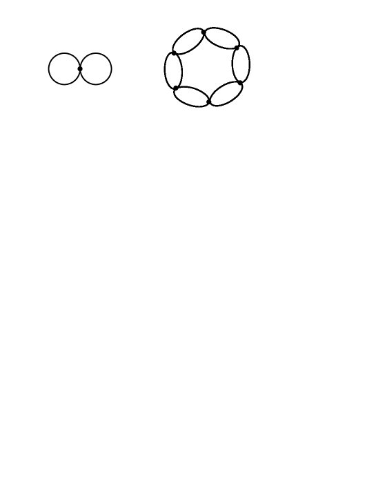
Figure 1: The contributions to the free energy in the $1/N$ expansion: the left diagram represents the Hartree contribution; the right diagram is one of the infinite set of “ring diagrams”.

Combining the value $W^{(0)}$ obtained above, Eq. (19), with the gaussian integral (21), we obtain $W[j]$ at order $1/N$:

$$W[j]=\left({1\over 2}\sigma_{c}^{2}+j\sigma_{c}\right)\beta L-\ln{{\cal Z}_{\sigma_{c}}\over{\cal Z}_{0}}+{\beta L\over 2}\int[d^{2}Q]\,\ln\left(1+g^{2}\Pi(Q)\right)\equiv W^{(0)}+W^{(1)}.$$ (24)

By taking the derivative of $W[j]$ in Eq. (24) with respect to $j$, one obtains $\bar{\sigma}$, the expectation value of the field $\sigma$. (Note that $\sigma_{c}$ depends implicitly on $j$ through the gap equation (15).) We can write $\bar{\sigma}=\sigma_{c}+\delta\bar{\sigma}$, and it follows immediately from Eqs. (24) and (15) that $\delta\bar{\sigma}$ is of order $1/N$ relative to $\sigma_{c}$. In computing the Legendre transform $\Gamma[\bar{\sigma}]=W^{(0)}+W^{(1)}-j\bar{\sigma}\beta L$ (see Eq. (12)), we may simply replace $\sigma_{c}$ by $\bar{\sigma}$, since the error made is of order $1/N^{2}$ (the terms linear in $\delta\bar{\sigma}$ drop in $W^{(0)}$ because $\sigma_{c}$ satisfies the gap equation (15); similarly, one makes an error of order $1/N^{2}$ in ignoring $\delta\bar{\sigma}$ in $W^{(1)}$ which is already a quantity of order $1/N$). The elimination of $j$ is then straightforward and we finally obtain the effective potential in the form:

$$V(M)=N{M^{2}\over 2g^{2}}-N\int\{d^{2}P\}\ln\left(1-{M^{2}\over P^{2}}\right)+{1\over 2}\int[d^{2}Q]\,\ln\left(1+g^{2}\Pi(Q)\right),$$ (25)

where $M$ is given by Eq. (17) with $\sigma$ replaced by $\bar{\sigma}$ . We shall write this effective potential as

$$V(M)=NV^{(0)}(M)+V^{(1)}(M),$$ (26)

where $NV^{(0)}(M)$ is the leading order contribution and $V^{(1)}(M)$ the next-to-leading order one. Before renormalization, $NV^{(0)}(M)$ is the sum of the first two terms in Eq. (25), and $V^{(1)}(M)$ is the last term. After renormalization, as we shall see, the first term in Eq. (25) contributes also at order $1/N$. For this reason, we shall often refer to the first two terms in Eq. (25) as the “fermionic” contribution, and to the last term as the “bosonic” one: the first two terms represent indeed the free energy density of massive fermions in the “Hartree approximation” BR86 , while the last term may be viewed as a the one-loop contribution of the bosonic degrees of freedom associated with the $\sigma$ field. In terms of the fermionic variables of the original lagrangian, the corresponding contributions to the free energy can be given a simple diagrammatic interpretation: the first diagram in Fig. 1 corresponds to the Hartree contribution, the second is one of the family of “ring diagrams” representing the bosonic contribution.

Before closing this subsection, let us recall that the effective potential is the generating functional of the irreducible $n$-point functions for the $\sigma$ field at zero momentum. In particular, the following, leading order, relation for the 2-point function can be easily established at zero temperature:

$$g^{2}{{\rm d}^{2}V^{(0)}\over{\rm d}M^{2}}=D^{-1}(Q=0;M)$$ (27)

where $D^{-1}=1+g^{2}\Pi$ is the inverse of the $\sigma$ propagator (see Eq. (23)). The same relation holds at finite temperature, but care must be exerted in specifying the limit $Q\to 0$ which is in general non analytic (it depends on which limit $\omega\to 0$ and $q\to 0$ is taken first). Thus, at finite temperature, the right hand side of the relation (27) has to be understood as $\lim_{q\to 0}D^{-1}(\omega\!=\!0,q;M)$ (see subsection V.2 and App. A).

II.2 Gap equation and quark condensate

As we have argued before, the equilibrium state is obtained by minimizing the effective potential with respect to $M$. One gets then the gap equation in the form:

$$0=\left.{dV\over dM}\right|_{M_{min}}={NM_{min}\over g^{2}}+\langle\bar{\psi}\psi\rangle_{M_{min}},$$ (28)

where we have used the fact that $\langle\bar{\psi}\psi\rangle$ may be obtained as the derivative with respect to $M$ of the last two terms in Eq. (25) (this may be seen by going back to the expression (6) of the partition function and using the fact that $\langle\bar{\psi}\psi\rangle$ can be obtained by differentiating ${\cal Z}_{\sigma}$ in Eq. (7) with respect to $\sigma$; see also Eq. (15) ). Thus, the value of $M$ at the minimum of the potential and the value of the quark-condensate in equilibrium are proportional:

$$M_{min}=-{g^{2}\over N}\langle\bar{\psi}\psi\rangle_{M_{min}},$$ (29)

which indicates that $\bar{\sigma}$ (or $M$) and $\langle\bar{\psi}\psi\rangle$ are equivalent order parameters for the discrete chiral symmetry.

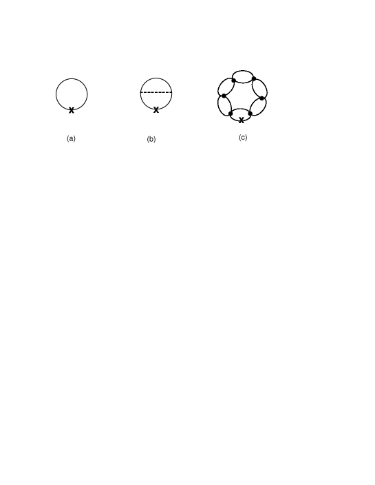
Figure 2: The fermion condensate $\langle\bar{\psi}\psi\rangle$: (a) leading order; (b) $1/N$ correction, the dashed line represents the $\sigma$ propagator; (c) same as (b) in the fermionic language.

We shall solve Eq. (28) order by order in the $1/N$ expansion. To do so, we write:

$$M_{min}=M_{min}^{(0)}+{1\over N}M_{min}^{(1)}.$$ (30)

In leading order, we have:

$$0=\left.{{\rm d}V^{(0)}\over{\rm d}M}\right|_{M_{min}^{(0)}}={M_{min}^{(0)}\over g^{2}}+{\langle\bar{\psi}\psi\rangle_{M_{min}^{(0)}}\over N},$$ (31)

where $\langle\bar{\psi}\psi\rangle_{M_{min}^{(0)}}$ is obtained from Eq. (18) with $M_{min}^{(0)}$ substituted for $M$. This gap equation needs to be solved exactly in order to get $M_{min}^{(0)}$. The correction $M_{min}^{(1)}$ is obtained by solving Eq. (28) to $1/N$ accuracy. We get then:

$$M_{min}^{(1)}=-{\left.{{\rm d}V^{(1)}\over{\rm d}M}\right|_{M_{min}^{(0)}}\over\left.{{\rm d}^{2}V^{(0)}\over{\rm d}M^{2}}\right|_{M_{min}^{(0)}}}.$$ (32)

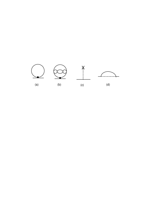
Figure 3: Contributions to the fermion mass. (a) leading order; (b) $1/N$ correction to the minimum of the effective potential; equivalently, the sum of the contributions (a) and (b) can be represented by diagram (c) where the insertion with a cross represents $M_{min}$. Diagram (d) represents an additional $1/N$ correction coming from $\Sigma$. As in Fig. 2, the dashed line in (d) represents the $\sigma$ propagator

To the expansion (30) of $M_{min}$ corresponds, according to Eq. (29), a similar expansion of the quark condensate:

$$\langle\bar{\psi}\psi\rangle=N\langle\bar{\psi}\psi\rangle^{(0)}+\langle\bar{\psi}\psi\rangle^{(1)}.$$ (33)

The two contributions to the quark condensate correspond to the diagrams displayed in Fig. 2. The leading order $\langle\bar{\psi}\psi\rangle^{(0)}$ corresponds to the contribution of the first diagram evaluated for $M_{min}=M_{min}^{(0)}$. The order $1/N$ correction $\langle\bar{\psi}\psi\rangle^{(1)}$ contains the contribution

$${dV^{(1)}\over dM}={1\over 2}\int[d^{2}Q]\,{\partial\Pi/\partial M\over 1+g^{2}\Pi(Q)}$$ (34)

associated with either of the last two diagrams in Fig. 2. In addition, as explicitly indicated in Eq. (32), $\langle\bar{\psi}\psi\rangle^{(1)}$ receives also a contribution from the first diagram in Fig. 2 evaluated at $M_{min}\neq M_{min}^{(0)}$.

Before closing this subsection, it is worth emphasizing that neither the minimum $M_{min}$ of the effective potential, nor the quark condensate are physical observables: after renormalization, and beyond leading order in the $1/N$ expansion, their values will depend on the renormalization scale.

II.3 The quark mass $M_{f}$

As we have mentioned, chiral symmetry is spontaneously broken in the ground state, and because of their coupling to the condensate the quarks acquire a mass. This mass is a physical quantity that we shall denote throughout as $M_{f}$. That is, $M_{f}$ will consistently refer to the mass of the quark in the vacuum, a quantity to be kept constant at all orders of our approximations.

In leading order in the $1/N$ expansion, the coupling to the condensate is the only contribution to the fermion mass and we can identify $M_{min}^{(0)}$ with $M_{f}$. This identification between $M_{min}$ and $M_{f}$ does not hold in higher order. Starting at order $1/N$, there are other contributions to the fermion mass besides $M_{min}$. Quite generally, the fermion mass is given by the pole of the fermion propagator at $P_{E}^{2}=-M_{f}^{2}$. The fermion propagator itself, $S(P)$, can be written as

$$S^{-1}(P)=S^{-1}_{\sigma}(P)+\Sigma(P)=-\hbox to0.0pt{\hbox to7.80904pt{\hfil/\hfil}\hss}P+M_{min}+\Sigma(P).$$ (35)

The various Feynman diagrams contributing to the fermion mass are displayed in Fig. 3. In leading order, $\Sigma(P)=0$. At next-to-leading order, $\Sigma(P)$ can be written as:

$$\Sigma(P)=a\hbox to0.0pt{\hbox to7.80904pt{\hfil/\hfil}\hss}P+b,$$ (36)

where $a$ and $b$ are functions of $P$ given in App. C. The equation $S^{-1}(\hbox to0.0pt{\hbox to7.80904pt{\hfil/\hfil}\hss}P=M_{f})=0$ yields then $M_{f}$ as a sum of two contributions:

$$M_{f}=M_{min}+M_{\Sigma},$$ (37)

where $M_{\Sigma}$ (which is of order $1/N$) is calculated in App. C.

At finite temperature, we shall define a temperature dependent mass $M_{f}(T)$ by the equation:

$$S^{-1}(\omega=M_{f}(T),p=0;T)=0.$$ (38)

where $S(\omega,p;T)$ is the fermion propagator at finite temperature. At leading order in the $1/N$ expansion $\Sigma(\omega,p;T)=0$, and one can simply identify the fermion mass $M_{f}(T)$ with the minimum of the finite temperature effective potential. At next-to-leading order, the evaluation of the $M_{f}(T)$ would require the calculation of $\Sigma(\omega,p;T)$. But, as we shall see in the following sections, this is not needed to evaluate the pressure at next-to-leading order.

III The renormalized effective potential at $T=0$

As we have already mentioned, the formulae given in the previous section contain ultraviolet divergent integrals. We discuss now the procedure of renormalization which allows us to get rid of the infinities. First we need to specify our regularization: this will consist in a simple cut-off $\Lambda$ on the length of the Euclidean momenta (for a discussion of more sophisticated regularizations in this type of models, see e.g. Ref. Ripka:zb ). We then obtain the effective potential as a function $V_{B}(M_{B};g_{B},\Lambda)$, referred to as the “bare” potential; the variables $\sigma_{B}$ (or $M_{B}$) and $g_{B}$, are the bare field (or mass) and coupling constant, respectively.

Divergent integrals appear in ${\rm d}V_{B}/{\rm d}M_{B}$ and ${\rm d}^{2}V_{B}/{\rm d}M_{B}^{2}$, i.e., in the one and two-point functions of the $\sigma$-field. The corresponding diagrams at leading order and at next-to-leading order are displayed in Fig. 4. Besides, there are divergences which are independent of $M_{B}$; these are eliminated by subtracting from $V_{B}(M_{B};g_{B},\Lambda)$ a constant $C(g_{B},\Lambda)$.

In order to construct the renormalized effective potential, we define a renormalized field $\sigma$, a renormalized coupling constant $g$, and a renormalized mass $M$ (related to $\sigma$ and $g$ by Eq. (17)). We set:

$$\sigma_{B}=\sqrt{Z}\sigma,\hskip 56.9055ptg_{B}=\sqrt{{Z^{\prime}\over Z}}g,\qquad\qquad M_{B}=\sqrt{Z^{\prime}}M.$$ (39)

where the renormalization constants $Z$ and $Z^{\prime}$ are dimensionless functions of the renormalized coupling $g$, and the cut-off $\Lambda$. These functions may be expanded in powers of $1/N$:

$$Z=Z^{(0)}+{1\over N}Z^{(1)},\qquad\qquad\qquad Z^{\prime}=Z^{\prime(0)}+{1\over N}Z^{\prime(1)},$$ (40)

and chosen so as to absorb the ultraviolet divergences at each order. Because they are dimensionless, $Z$ and $Z^{\prime}$ can actually depend only on the ratio of $\Lambda$ to another mass scale $M_{0}$, to be referred to as the renormalization scale, at which the renormalized $n$-point functions are specified (see below). In fact, we shall find convenient to consider $Z$ and $Z^{\prime}$ as functions of both $\Lambda/M_{f}$, where $M_{f}$ is the fermion mass, and $M_{0}/M_{f}$ (the latter quantity being eventually a finite function of the renormalized coupling): the dependence in $\Lambda$ will be fixed by the elimination of ultraviolet divergences, that on $M_{0}$ will be determined by renormalization conditions that we now present.

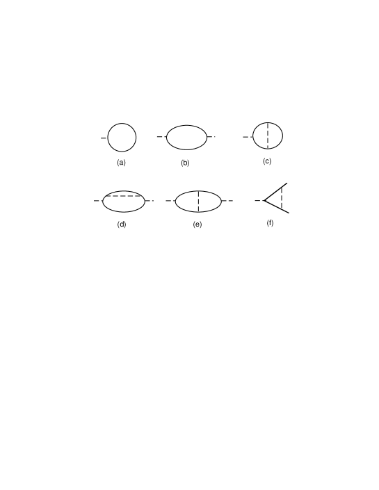
Figure 4: One-point (a,c) and two-point (b,d,e) functions for the $\sigma$ field, in leading order in the $1/N$ expansion (a,b), and at order $1/N$ (c,d,e). Diagram (f) is the first correction to the quark-sigma vertex; it is of order $1/N$. The dashed lines represent $\sigma$ propagators.

To this aim, we note first that the correction to the vertex $\sigma\bar{\psi}\psi$ is of order $1/N$ (see Fig. 4 f). In leading order, this vertex is therefore not renormalized and we may choose to balance the renormalization of the field with that of the coupling constant, i.e., set $g_{B}\sigma_{B}=g\sigma$ or equivalently, according to Eq. (39), set $Z^{\prime(0)}=1$. As for the constant $Z^{(0)}$, it will be determined by the following condition:

$$\left.{{\rm d}^{2}V^{(0)}\over{\rm d}M^{2}}\right|_{M_{0}}={1\over g^{2}}.$$ (41)

According to the relation (27) (extended to the corresponding renormalized quantities) this is equivalent to the condition $D(Q^{2}=0;M_{0})=1$ for the renormalized $\sigma$ propagator. At next-to-leading order we shall impose Coleman:jx that the first and second derivatives of the potential at $M=M_{0}$ are not changed by the $1/N$ corrections, that is:

$$\left.{{\rm d}V^{(1)}\over{\rm d}M^{2}}\right|_{M_{0}}=0,\qquad\qquad\left.{{\rm d}^{2}V^{(1)}\over{\rm d}M^{2}}\right|_{M_{0}}=0.$$ (42)

Summarizing the procedure that we have outlined, we may write the renormalized effective potential $V$ as follows:

$$V(M;g,M_{0})=V_{B}(M_{B};g_{B},\Lambda)-C(g_{B},\Lambda).$$ (43)

By construction, the right hand side has a finite limit when the cut-off $\Lambda$ is sent to infinity. For large $\Lambda$, the renormalized potential becomes therefore independent of $\Lambda$, i.e., it satisfies the renormalization group equation $\Lambda{{\rm d}V}/{{\rm d}\Lambda}=0,$ where the derivative is taken at fixed values of the renormalized quantities, and fixed $M_{0}$. This can be written explicitly as

$$\left[\Lambda{\partial\over\partial\Lambda}+\beta(g_{B}){\partial\over\partial g_{B}}-\gamma(g_{B})M_{B}{\partial\over\partial M_{B}}\right]\left(V_{B}(M_{B};g_{B},\Lambda)-C(g_{B},\Lambda)\right)=0,$$ (44)

where

$$\beta(g_{B})\equiv\Lambda{\partial g_{B}\over\partial\Lambda}={g_{B}\over 2}\,{\partial\ln(Z^{\prime}/Z)\over\partial\ln\Lambda}\,,\qquad\qquad\gamma(g_{B})\equiv-{\Lambda\over M_{B}}{\partial M_{B}\over\partial\Lambda}=-{1\over 2}{\partial\ln Z^{\prime}\over\partial\ln\Lambda}.$$ (45)

Alternatively, expressing the fact that the renormalized potential in Eq. (43) does not depend on the scale $M_{0}$, one can write the renormalization group equation as $M_{0}\,{{\rm d}V}/{{\rm d}M_{0}}=0,$ where the derivative is now taken at fixed bare quantities, and fixed cut-off $\Lambda$. Explicitly:

$$\left[M_{0}{\partial\over\partial M_{0}}+\beta(g){\partial\over\partial g}-\gamma(g)M{\partial\over\partial M}\right]V(M;g,M_{0})=0,$$ (46)

where

$$\beta(g)\equiv M_{0}{\partial g\over\partial M_{0}}={g\over 2}\,{\partial\ln(Z/Z^{\prime})\over\partial\ln M_{0}}\,,\qquad\qquad\gamma(g)\equiv-{M_{0}\over M}{\partial M\over\partial M_{0}}={1\over 2}{\partial\ln Z^{\prime}\over\partial\ln M_{0}}.$$ (47)

These various functions will be calculated in subsection III.3, where we shall also discuss some consequences of the renormalization group equations. We note here a general feature of the model that is useful to keep in mind in order to understand the logic of the construction of the effective potential in the next subsections. The model depends initially on two parameters, the bare coupling $g_{B}$ and the cut-off $\Lambda$. Since these will be adjusted so as to reproduce the fermion mass $M_{f}$, $g_{B}$ will become effectively a function of $\Lambda$. This relation between $g_{B}$ and $\Lambda$ depends on the accuracy with which $M_{f}$ is calculated, and is therefore modified at each order in the $1/N$ expansion. The same property holds in the renormalized theory: there exists a relation between the renormalized coupling $g$ and the scale $M_{0}$, which is redefined at each order so that the calculation of the fermion mass at that order reproduces the value $M_{f}$.

We shall, in the next two subsections, construct the leading and next-to-leading order contributions to the renormalized effective potential. We shall see that it is possible to write these in terms of a variable $x_{M}$ related to $M$, but which is invariant under renormalization group transformations ($M$ is not invariant beyond leading order). This choice of variable will make it obvious that the potential is independent of $M_{0}$, and it follows from the relation between $M_{0}$ and $g$ alluded to above, that it will be also independent of the renormalized coupling.

III.1 The leading order contribution

The zeroth order in the $1/N$ expansion of the potential, $V^{(0)}_{B}$, is the fermionic contribution in Eq. (25). At T=0 it can be written as:

$$NV^{(0)}_{B}(M_{B}) = N{1\over 2g_{B}^{2}}M_{B}^{2}-N\int{d^{2}p\over(2\pi)^{2}}\ln\left(1-{M_{B}^{2}\over P^{2}}\right).$$ (48)

This expression is divergent. Introducing a cut-off $\Lambda$ on the length of the Euclidean momentum ($\sqrt{P_{E}^{2}}<\Lambda$), one obtains:

$$V^{(0)}_{B}(M_{B})={M_{B}^{2}\over 2g_{B}^{2}}+{M_{B}^{2}\over 4\pi}\left(\ln{M_{B}^{2}\over\Lambda^{2}}-1\right)+{\cal O}\left({M_{B}^{2}\over\Lambda^{2}}\right).$$ (49)

We proceed now to the renormalization of the potential along the lines described in the previous section. Since at leading order $Z^{\prime}=Z^{\prime(0)}$=1 (see the discussion after Eq. (40)), we can simply replace $M_{B}$ by $M$, and we need only to renormalize the coupling constant. After this, there will be no need for further subtraction. By expressing $g_{B}$ in terms of $g$ in Eq. (49), using Eq. (39) with $Z=Z^{(0)}$, we get:

$$V^{(0)}(M)={Z^{(0)}M^{2}\over 2g^{2}}+{M^{2}\over 4\pi}\left(\ln{{M^{2}\over\Lambda^{2}}}-1\right).$$ (50)

The $\Lambda$-dependent term is eliminated by choosing

$$Z^{(0)}={g^{2}\over 2\pi}\ln{\Lambda^{2}\over M_{f}^{2}}+\bar{Z}^{(0)},$$ (51)

where the finite constant $\bar{Z}^{(0)}$ is fixed by the renormalization condition (41):

$$\bar{Z}^{(0)}(M_{0},g)=1-g^{2}/\pi+(g^{2}/\pi)\ln(M_{f}/M_{0}).$$ (52)

The renormalized potential at leading order can then be written as:

$$V^{(0)}(M)={M^{2}\over 2g^{2}}\bar{Z}^{(0)}+{M^{2}\over 4\pi}\left(\ln{M^{2}\over M_{f}^{2}}-1\right)={M^{2}\over 4\pi}\left(\ln{M^{2}\over M_{0}}-3+{2\pi\over g^{2}}\right).$$ (53)

It has two minima, at $\pm M_{min}^{(0)}$, with:

$$M_{min}^{(0)}(M_{0},g)=M_{f}\,{\rm e}^{-(\pi/g^{2})\bar{Z}^{(0)}}=M_{0}\,{\rm e}^{1-\pi/g^{2}}.$$ (54)

The existence of such non trivial minima of the effective potential indicates spontaneous symmetry breaking with, according to Eq. (29), a non vanishing value of the quark condensate.

It remains to verify that $V^{(0)}$ does not depend on $M_{0}$. To do so, we remind first that, at this order, we can set $M_{min}^{(0)}=M_{f}$, or equivalently (see Eq. (54)) $\bar{Z}^{(0)}=0$. Then, one gets:

$$V^{(0)}(M)={M^{2}\over 4\pi}\left(\ln{M^{2}\over M_{f}^{2}}-1\right)={M_{f}^{2}\over 4\pi}\,x_{M}(\ln x_{M}-1),$$ (55)

where we have set

$$x_{M}\equiv M^{2}/M_{f}^{2}.$$ (56)

Since at this order $M$ is not renormalized, the variable $x_{M}$ is clearly a renormalization group invariant, and so is the effective potential. At next-to-leading order, we shall see that it is still possible to express the effective potential in terms of a renormalization group invariant $x_{M}$ whose definition generalizes that in Eq. (56) so as to include an $M_{0}$-dependent correction of order $1/N$ (this correction will compensate the $M_{0}$-dependence of $M$; see Eq. (86)). We note also that, as expected from the discussion at the end of the previous subsection, the expression (55) of the effective potential does not depend on the coupling constant anymore: by eliminating the explicit dependence on $M_{0}$, we have also eliminated the dependence on $g$.

In order to get the expression (55) of the effective potential, we did not need the explicit expression of $\bar{Z}^{(0)}$ given by Eq. (52). This is needed however to specify the explicit relation between $M_{0}$ and $g$. From the equation $M_{f}=M_{min}^{(0)}(M_{0},g)$, or equivalently $\bar{Z}^{(0)}(M_{0},g)=0$, one gets:

$$g^{2}(M_{0})={\pi\over 1+\ln(M_{0}/M_{f})}\,.$$ (57)

This formula indicates that $g$ becomes vanishingly small as $M_{0}\to\infty$, as expected from asymptotic freedom. It also shows that $g$ diverges when $M_{0}\to M_{f}/e$, a property that we shall discuss further shortly.

Before we do that, we note that the main results obtained so far in this subsection could be derived by working solely with the bare quantities. In terms of the bare parameters and the cut-off $\Lambda$, the minima of $V^{(0)}_{B}(M_{B})$ are given by the solutions of the gap equation:

$${M_{B}\over g_{B}^{2}}={M_{B}\over 4\pi}\ln\left({\Lambda^{2}\over M_{B}^{2}}\right).$$ (58)

The right hand side of this equation is $-\langle\bar{\psi}\psi\rangle/N$, i.e., it is proportional to the quark condensate (see Eq. (28)). Aside from the trivial solution $M_{B}=0$, the gap equation has two degenerate solutions at $M_{B}=\pm M_{min}^{(0)}$ with:

$$M_{\rm min}^{(0)}(\Lambda,g_{B})=\Lambda{\rm e}^{-\pi/g^{2}_{B}}.$$ (59)

By identifying one of the non trivial solutions with the fermion mass, as we did above, e.g. setting $M_{f}=M_{\rm min}^{(0)}(\Lambda,g_{B})$, we get the relation between the bare coupling and the cut-off:

$$g_{B}^{2}={\pi\over\ln\Lambda/M_{f}}\,.$$ (60)

This may be used to eliminate $\Lambda$ from the expression (49) of the potential and recover Eq. (55) (recall that at this order $M_{B}=M$).

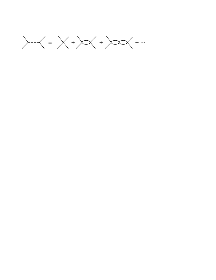
Figure 5: The quark-quark scattering amplitude corresponding to the exchange of a $\sigma$ meson (left-hand side), and its expression in terms of the fermionic variables.

We end this subsection by considering the quark-quark scattering amplitude ${\cal T}(\omega,q;M)$, where the quark mass $M$ is considered as an independent parameter. In leading order (in perturbation theory) this scattering amplitude is simply the bare coupling constant squared $g_{B}^{2}$. Including the exchange of the $\sigma$ meson, which contributes at the same order as the bare coupling in the $1/N$ expansion, one obtains:

$${\cal T}(Q_{E};M)={g_{B}^{2}\over 1+g_{B}^{2}\Pi_{0}(Q_{E};M)}.$$ (61)

A diagrammatic interpretation of ${\cal T}(Q_{E};M)$ is given in Fig. 5. The scattering amplitude can also be expressed in terms of renormalized quantities (see App. A):

$${\cal T}(Q_{E};M)=g^{2}\,D_{0}(Q_{E};M),$$ (62)

where $g^{2}$ is the square of the renormalized coupling constant at the scale $M_{0}$, i.e., $g^{2}=g^{2}(M_{0}^{2})$ (given by Eq. (57)) and $D_{0}$ is the renormalized $\sigma$ propagator (given by Eq. (196)). Note that the explicit $g^{2}$ in the r.h.s. of Eq. (62) cancels with the factor $1/g^{2}$ contained in $D_{0}$ (see Eq. (196)) so that ${\cal T}(Q_{E};M)$ is independent of the renormalisation scale $M_{0}$, i.e., the scattering amplitude is a renormalization group invariant. Using the explicit expression of $D_{0}(Q_{E};M)$ given in App. A, one easily shows that ${\cal T}(Q_{E}=0;M_{f})=g^{2}(M^{2})$, and that at large $Q_{E}^{2}$ ($Q_{E}^{2}\gg M_{f}^{2}$, $M\mathrel{\hbox to0.0pt{\raise 2.20013pt\hbox{$<$}\hss}{\lower 2.20013pt\hbox{$\sim$}}}M_{f}$), ${\cal T}(Q_{E};M_{f})\approx 2\pi/\ln(Q_{E}^{2}/M_{f}^{2})\approx g^{2}(Q_{E}^{2})$. This logarithmic decrease of the interaction strength at large $Q_{E}^{2}$ reflects of course the property of asymptotic freedom.

As explained in App. A (see Eq. (196) and the discussion that follows), the $\sigma$ propagator develops a pole at finite $Q_{E}$ when $M<M_{f}/e$ and, according to Eq. (62), so does the quark-quark scattering amplitude. This pole which does not correspond to a physical excitation of the system is commonly referred to as a Landau pole; as we shall see, it is responsible for several difficulties in our next-to-leading order calculation at finite temperature. We shall denote by $M_{*}$ the value of $M$ at which the Landau pole appears at $Q_{E}=0$. Here $M_{*}=M_{f}/e$. As we have seen before, at $Q_{E}=0$ the scattering amplitude is simply ${\cal T}(Q_{E}=0;M)=g^{2}(M^{2})$ which diverges when $M\to M_{*}$ (see Eq.  (57)). Since ${\cal T}(Q_{E}=0;M)$ is nothing but the inverse of the second derivative of the leading order effective potential $V^{(0)}$ (see Eqs. (27) and (62), and also (197)), $M_{*}$ is also the zero of the second derivative of (55). At zero temperature, $M_{*}$ is far from the physical quark mass $M_{f}$, and the quantum fluctuations of the $\sigma$ field do not probe values of $M$ close to $M_{*}$; the Landau pole is then harmless. We shall see that this is no longer the case at finite temperature.

III.2 The $1/N$ contribution

We consider now the next-to-leading order contributions to the effective potential. There are two such contributions that we call $V^{(1)}_{f}$ and $V^{(1)}_{b}$. The latter is the bosonic contribution, i.e., the last term in Eq. (25). In terms of bare quantities, this reads:

$$V^{(1)}_{b,B}(M_{B};g_{B},\Lambda)={1\over 2}\int^{\Lambda}{d^{2}q\over(2\pi)^{2}}\ln\left[1+g_{B}^{2}\Pi_{0}(Q_{E};M_{B},\Lambda)\right],$$ (63)

where the cut-off $\Lambda$ applies to the magnitude $\sqrt{Q_{E}^{2}}$ of the Euclidean momentum, and $\Pi_{0}(Q_{E};M_{B},\Lambda)$ is given in App. A. The other contribution, $V^{(1)}_{f}$, originates from the renormalization of the coupling constant $g_{B}$ and the mass $M_{B}$, at next-to-leading order, in the fermionic contribution, Eq. (49). It will be examined later in this section.

We first address the problem of finding a constant $C(g_{B},\Lambda)$ to eliminate the $M$-independent divergences of $V^{(1)}_{b,B}$. We define:

$$C(g_{B},\Lambda)={1\over 2}\int^{\Lambda}{d^{2}q\over(2\pi)^{2}}\ln\left[1+g_{B}^{2}\Pi_{0}(Q_{E};M_{\Lambda},\Lambda)\right]-{M_{\Lambda}^{2}\over 4\pi}\ln{\Lambda^{2}\over M_{\Lambda}^{2}}\,-{M_{\Lambda}^{2}\over 4\pi}\ln\ln{\Lambda\over M_{\Lambda}}.$$ (64)

with $M_{\Lambda}\equiv\Lambda{\rm e}^{-\pi/g_{B}^{2}}$, and we verify now that this subtraction fulfills our requirements. First, we express $V^{(1)}_{b,B}(M_{B};g_{B},\Lambda)-C(g_{B},\Lambda)$ in terms of the renormalized mass and coupling constant according to Eqs. (39). Note that since $V^{(1)}_{b}$ is already of order $1/N$, we need only the leading order renormalization constants. That is, we can set $M_{B}=M$ and $g^{2}_{B}=g^{2}/Z^{(0)}$, with $Z^{(0)}$ given by Eq. (51) with $\bar{Z}^{(0)}=0$. Furthermore, we can also replace $M_{\Lambda}=\Lambda e^{-\pi/g_{B}^{2}}$ by $M_{f}$, using the relation (59) and the identification at leading order of $M_{min}^{(0)}$ with $M_{f}$. Thus, at this stage:

$$V^{(1)}_{b}(M)={1\over 2}\int^{\Lambda}{d^{2}q\over(2\pi)^{2}}\,\ln\left[{D^{-1}_{0}(Q_{E};M)\over D^{-1}_{0}(Q_{E};M_{f})}\right]+{M_{f}^{2}\over 4\pi}\ln{\Lambda^{2}\over M_{f}^{2}}\,+{M_{f}^{2}\over 4\pi}\ln\ln{\Lambda\over M_{f}}.$$ (65)

where $D^{-1}_{0}(Q_{E};M)=Z^{(0)}+g^{2}\Pi_{0}(Q_{E};M,\Lambda)$ is the renormalized inverse $\sigma$ propagator given by Eq. (196).

The integrand in Eq. (65) vanishes when $Q_{E}^{2}\to\infty$, but not fast enough to make the integral convergent as $\Lambda\to\infty$. Indeed, from (198) one gets

$${D^{-1}_{0}(Q_{E};M)\over D^{-1}_{0}(Q_{E};M_{f})}\simeq 1+{2{\cal A}(M)\over Q_{E}^{2}}+{2{\cal B}(M)\over Q_{E}^{2}\ln(Q_{E}^{2}/M_{f}^{2})}+{\cal O}\left({M^{4}\over Q_{E}^{4}\ln(Q_{E}^{2}/M_{f}^{2})}\right),$$ (66)

where:

$${\cal A}(M)=M^{2}-M_{f}^{2}\,,\qquad{\cal B}(M)=M^{2}-M_{f}^{2}-M^{2}\ln(M^{2}/M_{f}^{2})\,.$$ (67)

The terms proportional to ${\cal A}$ and ${\cal B}$ yield the following contributions to the integral:

$${{\cal A}(M)\over 4\pi}\ln{\Lambda^{2}\over M_{f}^{2}}\,,\qquad\qquad{{\cal B}(M)\over 4\pi}\ln\ln{\Lambda\over M_{f}},$$ (68)

which contain $M$-dependent but also $M$-independent divergences. The latter cancel exactly the last two terms of Eq. (65). The former contribute $M$-dependent terms to Eq. (65) which are of the same form as those of the leading order potential, $V^{(0)}$, namely $M^{2}$ and $M^{2}\ln M^{2}$ (see Eq. (50)), and they can be eliminated by an appropriate adjustment of the two renormalization constants $Z$ and $Z^{\prime}$. To see that, we need to return to the leading order contribution to the bare potential, (Eq. (49)), and trade then $M_{B}$ and $g_{B}$ for $M$ and $g$, using Eqs. (39). We get:

$${M^{2}Z\over g^{2}}+{M^{2}Z^{\prime}\over 4\pi}\left(\ln\left({M^{2}Z^{\prime}\over\Lambda^{2}}\right)-1\right).$$ (69)

By expanding $Z$ and $Z^{\prime}$ up to order $1/N$ as in Eq. (40), one can write the above expression (69) as $V^{(0)}+({1}/{N})V^{(1)}_{f}$, with $V^{(0)}$ given by Eq. (53) and, dropping terms of order $1/N^{2}$,

$$V^{(1)}_{f}(M)=M^{2}\left({Z^{(1)}\over 2g^{2}}+{Z^{\prime(1)}\over 4\pi}\ln\left({M^{2}\over\Lambda^{2}}\right)\right).$$ (70)

As mentioned at the beginning of this section, $V^{(1)}_{f}(M)$ (from the equation above) adds to $V^{(1)}_{b}(M)$ (from Eq. (65)) to yield the complete next-to-leading order contribution to the renormalized potential, $V^{(1)}(M)=V^{(1)}_{f}(M)+V^{(1)}_{b}(M)$. The requirement that $\Lambda$ disappears from $V^{(1)}(M)$ then allows us to determine the $\Lambda$-dependence of the renormalization constants $Z^{(1)}$ and $Z^{\prime(1)}$. One gets:

$$Z^{(1)}={g^{2}\over 2\pi}\left[(Z^{\prime(1)}-1)\ln\left({\Lambda^{2}\over M_{f}^{2}}\right)-\ln\ln{\Lambda\over M_{f}}\right]+\bar{Z}^{(1)}$$ (71)

$$Z^{\prime(1)}=\ln\ln\left({\Lambda\over M_{f}}\right)+\bar{Z}^{\prime(1)},$$ (72)

where $\bar{Z}^{\prime(1)}$ and $\bar{Z}^{(1)}$ are finite constants to be fixed using the renormalization conditions (42). We postpone this determination till later. Keeping along $\bar{Z}^{\prime(1)}$ and $\bar{Z}^{(1)}$, one can then write the renormalized effective potential in the form:

$$V^{(1)}(M)=\bar{Z}^{(1)}{M^{2}\over 2g^{2}}+\bar{Z}^{\prime(1)}{M^{2}\over 4\pi}\ln{M^{2}\over M_{f}^{2}}-{1\over 2\pi}(M^{2}-M_{f}^{2})+{M_{f}^{2}\over 4\pi}F_{0}(x_{M}),$$ (73)

with $x_{M}=M^{2}/M_{f}^{2}$ (see Eq. (56)), and $F_{0}(x)$ is a finite function defined in App. B.

The renormalization conditions (42) needed to fix the finite constants ${\bar{Z}}^{(1)}$ and ${\bar{Z}}^{\prime(1)}$ require two derivatives of $V^{(1)}$. The first derivative of $V^{(1)}$ with respect to $M^{2}$ is easily obtained from (73):

$${dV^{(1)}\over dM^{2}}={\bar{Z}^{(1)}\over 2g^{2}}-{1\over 2\pi}+{\bar{Z}^{\prime(1)}\over 4\pi}(\ln x_{M}+1)+{1\over 4\pi}F_{0}^{\prime}(x_{M})$$ (74)

where $F_{0}^{\prime}={\rm d}F_{0}/{\rm d}x$. The second derivative of $V^{(1)}$ may be calculated as

$${d^{2}V^{(1)}\over dM^{2}}=2{dV^{(1)}\over dM^{2}}+4x_{M}{d\over dx_{M}}\left({dV^{(1)}\over dM^{2}}\right).$$ (75)

One thus easily gets:

$${d^{2}V^{(1)}\over dM^{2}}={\bar{Z}^{(1)}\over g^{2}}+{\bar{Z}^{\prime(1)}\over 2\pi}(\ln x_{M}+3)-{1\over\pi}+{1\over 2\pi}F_{0}^{\prime}(x_{M})+{x_{M}\over\pi}F_{0}^{\prime\prime}(x_{M}),$$ (76)

where $F_{0}^{\prime\prime}={\rm d}^{2}F_{0}/{\rm d}x^{2}$. The derivatives of $F_{0}(x)$ are given in App. B.

In this subsection we shall in fact only fix $\bar{Z}^{(1)}$ and leave $\bar{Z}^{\prime(1)}$ undetermined. The reason is that, as we shall see, it is not necessary to specify the value of $\bar{Z}^{\prime(1)}$ in order to get a renormalization group invariant expression for the effective potential. By imposing the second renormalization condition (42), viz $d^{2}V^{(1)}/dM^{2}=0$ at $M=M_{0}$, we can express $\bar{Z}^{(1)}$ in terms of $\bar{Z}^{\prime(1)}$. Using Eq. (76), one gets:

$$\bar{Z}^{(1)}={g^{2}\over 2\pi}\left(2-\bar{Z}^{\prime(1)}\left(3+\ln x_{0}\right)-F^{\prime}_{0}(x_{0})-2x_{0}F^{\prime\prime}_{0}(x_{0})\right),$$ (77)

where the quantity $x_{0}$ is the following function of $g$:

$$x_{0}\equiv{\rm e}^{2(\pi/g^{2}-1)}.$$ (78)

At leading order $x_{0}={M_{0}^{2}}/{M_{f}^{2}}$, as can be easily deduced from Eq. (57). We can then write the next-to-leading order contribution to the renormalized potential as follows:

$$V^{(1)}(M)={M^{2}\over 4\pi}\left[\bar{Z}^{\prime(1)}\left(\ln{M^{2}\over M_{f}^{2}}\!-\!3\!-\!\ln x_{0}\right)\!-\!F^{\prime}_{0}(x_{0})\!-\!2x_{0}F^{\prime\prime}_{0}(x_{0})\right]\!+\!{M_{f}^{2}\over 2\pi}+{M_{f}^{2}\over 4\pi}F_{0}(x_{M}).$$ (79)

The full renormalized potential up to next-to-leading order is thus $V=NV^{(0)}+V^{(1)}$ with $V^{(0)}$ and $V^{(1)}$ given by Eqs. (53) and (79), respectively.

The effective potential that we just constructed has an apparent dependence on the scale $M_{0}$. However, as we did in the leading order case, it is possible to exploit the relation between the fermion mass $M_{f}$ and the value $M_{min}$ of $M$ at the minimum of the effective potential, in order to get rid of this apparent $M_{0}$ dependence. The situation is somewhat more complicated here because, as explained in subsection II.2, the fermion mass receives two contributions at order $1/N$, $M_{min}$ and $M_{\Sigma}$. The latter is calculated in the App. C and takes the form:

$$M_{\Sigma}=M_{f}\left({\bar{Z}^{\prime(1)}\over 2N}+{\varphi\over N}\right),$$ (80)

where $\varphi$ is a numerical constant, $\varphi=-0.126229$ (see Eq. (249)) . The value of $M_{min}$ can be calculated by setting $M_{min}=M_{min}^{(0)}+({1}/{N})M_{min}^{(1)}$ (see Eq. (30)), with $M_{min}^{(0)}$ and $M_{min}^{(1)}$ given by Eqs. (54) and (32), respectively. The required derivative of $V^{(1)}$ can be obtained from Eq. (74) (together with (77)). Note also that $M_{min}^{(0)}=M_{f}+{\cal O}(1/N)$ and that, at the minimum, ${\rm d}^{2}V^{(0)}/{\rm d}M^{2}=1/\pi$. One thus gets:

$$M_{min}^{(1)}=M_{min}^{(0)}\left(\left({1\over 2}\ln x_{0}+1\right)\bar{Z}^{\prime(1)}+{1\over 2}F^{\prime}_{0}(x_{0})+x_{0}F^{\prime\prime}_{0}(x_{0})-{1\over 2}F^{\prime}_{0}(1)\right).$$ (81)

Remembering that $M_{f}=M_{min}+M_{\Sigma},$ (see Eq. (37)), and combining Eqs. (80) and (81), one can therefore write $M_{f}$ as:

$$M_{f}=M_{0}\,{1\over\sqrt{x}_{0}}\left[1+{1\over N}\left({\bar{Z}^{\prime(1)}\over 2}(\ln x_{0}+3)\!+\!{1\over 2}F^{\prime}_{0}(x_{0})+x_{0}F^{\prime\prime}_{0}(x_{0})\!-\!{1\over 2}F^{\prime}_{0}(1)\!+\!\varphi\right)\right].$$ (82)

For the purpose of eliminating $M_{0}$, it is convenient to rewrite Eq. (82) as follows (neglecting terms of order $1/N^{2}$):

$$\ln{M_{f}\over M_{0}}=-{1\over 2}\ln x_{0}+{1\over N}\left({\bar{Z}^{\prime(1)}\over 2}(\ln x_{0}+3)+{1\over 2}F^{\prime}_{0}(x_{0})+x_{0}F^{\prime\prime}_{0}(x_{0})-{1\over 2}F^{\prime}_{0}(1)+\varphi\right).$$ (83)

We shall return to this equation in subsection III.3 below. For the moment we note that it allows us to easily eliminate the term $\sim\ln M_{0}$ in the leading order potential $V^{(0)}(M)$ given in Eq. (53). Combining the resulting expression with Eq. (79) and droping again terms of order $1/N^{2}$ (in particular, using $x_{0}=M_{0}^{2}/M_{f}^{2}+O(1/N)$), one finally gets

$$V(M) = NV^{(0)}+V^{(1)}$$ (84)

$$= {NM^{2}\over 4\pi}\left(-1+\ln{M^{2}\over M_{f}^{2}}\right)+{M^{2}\over 4\pi}\left(\xi+\bar{Z}^{\prime(1)}\ln{M^{2}\over M_{f}^{2}}\right)+{M_{f}^{2}\over 2\pi}+{M_{f}^{2}\over 4\pi}F_{0}(x_{M}),$$

where $\xi\equiv 2\varphi-F^{\prime}_{0}(1)=-0.8661636$. At this point we observe that

$$\left(1+{\bar{Z}^{\prime(1)}\over N}\right)\ln{M^{2}\over M_{f}^{2}}-1=\left(1+{\bar{Z}^{\prime(1)}\over N}\right)\left[\ln\left({M^{2}\over M_{f}^{2}}\left(1+{\bar{Z}^{\prime(1)}\over N}\right)\right)-1\right]+{\cal O}(1/N^{2}).$$ (85)

This allows us to express the full effective potential $V$ entirely in terms of the redefined variable $x_{M}$:

$$x_{M}\equiv{M^{2}\over M^{2}_{f}}\left(1+{\bar{Z}^{\prime(1)}\over N}\right).$$ (86)

The final result for the effective potential can then be put in the form (with a slight abuse in the notation):

$$V(x_{M})={M_{f}^{2}\over 4\pi}\left[Nx_{M}(\ln x_{M}-1)+\xi(x_{M}-1)+F_{0}(x_{M})\right].$$ (87)

where we have explicitly subtracted the constant $2+\xi$ so that $V^{(1)}(x_{M}=1)=0$. Note that the definition of $x_{M}$ in Eq. (86) differs from that in Eq. (56) by a term of order $1/N$. There is no contradiction however since $F_{0}(x)$ is already of order $1/N$, so that using $x_{M}=M^{2}/M_{f}^{2}$ instead of the definition (86) inside $F_{0}(x_{M})$ is equivalent to ignoring terms of order $1/N^{2}$. We shall see in the next subsection that $x_{M}$ is a renormalization group invariant. The effective potential $V(x_{M})$ is thus explicitly independent of the scale $M_{0}$, and for the reasons discussed at the beginning of this section (after Eq. (47)), also independent of $g$. Note that in terms of the redefined variable $x_{M}$ (Eq. (86)), the leading order contribution in Eq. (87) is identical to that of Eq. (55).

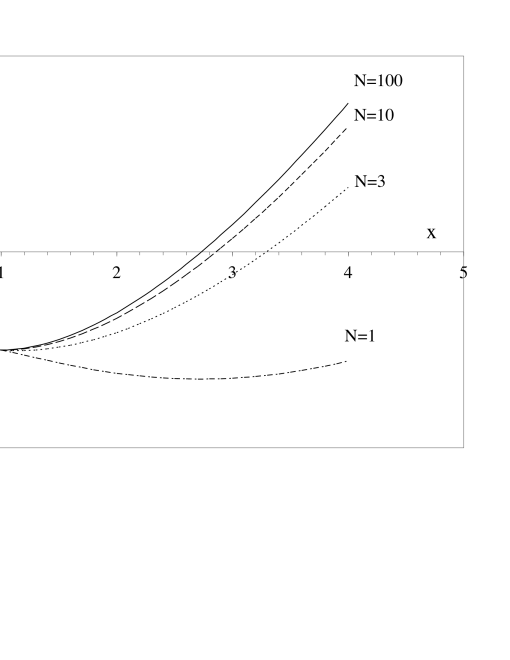
Figure 6: The effective potential divided by $NM_{f}^{2}/4\pi$ as a function of $x_{M}$ for the values $N=1$, $N=3$, $N=10$ and $N=100$. The minimum occurs at $x_{min}=2.721$ for $N=1$, $x_{min}=1.145$ for $N=3$, $x_{min}=1.068$ for $N=5$, $x_{min}=1.029$ for $N=10$, and $x_{min}\approx 1-2\varphi/N\approx 1+0.25/N$ for larger values of $N$. The $1/N$ correction has been adjusted so as to vanish at $x_{M}=1$; it also changes sign at this point.

The effective potential (87) is displayed in Fig. 6 for various values of $N$. One sees that the $1/N$ correction becomes rapidly a small correction. For $N=1$, the approximation is of course meaningless, but already for $N=3$, the shape of the potential is qualitatively the same as at leading order. The variation of the minimum with $N$ may be obtained as explained in Sect. II from the general equation (32):

$$x_{min}=1+{x_{min}^{(1)}\over N}\qquad\qquad x_{min}^{(1)}=-{\left.{{\rm d}V^{(1)}\over{\rm d}x_{M}}\right|_{x_{M}=1}\over\left.{{\rm d}^{2}V^{(0)}\over{\rm d}x_{M}^{2}}\right|_{x_{M}=1}}.$$ (88)

From the explicit expression (87) we get $\left.{{\rm d}^{2}V^{(0)}}/{{\rm d}x_{M}^{2}}\right|_{1}=M_{f}^{2}/4\pi$, and $\left.{{\rm d}V^{(1)}}/{{\rm d}x_{M}}\right|_{1}=(M_{f}^{2}/4\pi)(\xi+F^{\prime}_{0}(1))=\varphi M_{f}^{2}/2\pi$, so that, at next-to-leading order, $x_{min}=1-2\varphi/N\approx 1+0.25/N$. The difference between this value and that of the “exact” minimum found numerically from Eq. (87) can be attributed to terms of order $1/N^{2}$. As can be deduced from the caption of Fig. 6 for $N\mathrel{\hbox to0.0pt{\raise 2.20013pt\hbox{$>$}\hss}{\lower 2.20013pt\hbox{$\sim$}}}10$ these are small, confirming the previous study of Ref. Root:1974zr . (Of course, such considerations say very little about the magnitude of the true $1/N^{2}$ corrections.) It is interesting to recover the previous result for $x_{min}$ in a different way. Using the definition of $x_{M}$ in Eq. (86), we can write $M_{min}=\sqrt{x_{min}}\,M_{f}(1-\bar{Z}^{\prime(1)}/2N)$. The equation $M_{f}=M_{min}+M_{\Sigma}$ reads then:

$$M_{f}=M_{f}\left[1+{x_{min}^{(1)}\over 2N}-{\bar{Z}^{\prime(1)}\over 2N}\right]+M_{f}\left[{\bar{Z}^{\prime(1)}\over 2N}+{\varphi\over N}\right],$$ (89)

where we have used Eq. (80) for $M_{\Sigma}$ and the first equation in (88). Eq. (89) gives back our previous result $x_{min}^{(1)}=-2\varphi$. It also clearly illustrates how the scale dependence cancels out between $M_{min}$ and $M_{\Sigma}$, whereas the magnitude of each individual contribution depends on $M_{0}$ (through $\bar{Z}^{\prime(1)}$). We come back on this issue in the next subsection.

Note finally that the potential is plotted only for $x_{M}>1/e^{2}\equiv x_{M_{*}}$. This is because for $x_{M}<x_{M_{*}}$ a Landau pole appears in the $\sigma$ propagator (see subsection III.1), making the function $F_{0}$ complex (see Eq. (65) or, equivalently Eq. (B)). The influence of this Landau pole on the shape of the effective potential is clearly visible in Fig. 6 on the plot of $V(x_{M})$ for $N=1$: not only does the potential becomes complex for $x_{M}<x_{M_{*}}$, but the “$1/N$ correction” is large and negative for $x_{M}\mathrel{\hbox to0.0pt{\raise 2.20013pt\hbox{$>$}\hss}{\lower 2.20013pt\hbox{$\sim$}}}x_{M_{*}}$. As soon as $N>3$, however, this peculiar behavior is no longer visible.

III.3 Renormalisation group analysis

In this subsection, we shall clarify the behavior under renormalization group transformations of various quantities that have been introduced in the previous subsections. In particular we shall verify that the expression (82) of the fermion mass is invariant, and so is the variable $x_{M}$ defined in Eq. (86). But before we do that, let us verify that our calculation reproduces known results for the renormalization group functions.

The functions $\beta$ and $\gamma$ are most easily obtained by differentiating the renormalization constants with respect to the cut-off $\Lambda$, according to Eq. (45). Using Eqs. (51), (71) and (72) one easily gets:

$$\beta(g_{B})=\beta^{(0)}(g_{B})+{1\over N}\,\beta^{(1)}(g_{B}),$$ (90)

with

$$\beta^{(0)}(g_{B})=-{g_{B}^{3}\over 2\pi},\qquad\beta^{(1)}(g_{B})={g_{B}^{3}\over 2\pi}+{g_{B}^{5}\over 4\pi^{2}}.$$ (91)

Eqs. (90) and (91) show that, for $N=1$, the leading term in a small $g$-expansion (i.e., that of order $g^{3}$) in the $\beta$-function vanishes. This is in agreement with earlier calculations and the fact that for $N=1$ the Gross-Neveu model reduces to the Thirring model Thirring:in , for which the $\beta$-function vanishes identically. (The term of order $g^{5}$ does not vanish when $N=1$ in Eq. (91) because the $1/N$ correction does not contain all the terms of order $g^{5}$ in the small $g$ limit). The two-loop $\beta$-function has been calculated by Wetzel Wetzel:1984nw and reads $\beta(g)=-(1-1/N)(g^{3}/2\pi)+(1/N-1/N^{2})(g^{5}/4\pi^{2})$). Note finally that $\beta^{(0)}(g_{B})$ follows immediately from the explicit relation (60) between $g_{B}$ and the cut-off $\Lambda$.

Following similar steps, one obtains the function $\gamma\equiv\gamma^{(0)}+(1/N)\gamma^{(1)}$. Since at leading order, $Z^{\prime}=1$, $\gamma^{(0)}(g_{B})=0$. Using Eq. (72) and also the relation (60) between the cut-off $\Lambda$ and the bare coupling constant we get:

$$\gamma^{(1)}(g_{B})=-{g_{B}^{2}\over 2\pi}.$$ (92)

It is instructive to repeat the calculation of the renormalization group functions by differentiating with respect to $M_{0}$. The calculation is more involved because $M_{0}$ enters the finite parts of the renormalization constants. The calculation of $\beta^{(0)}(g)$ is trivial however and reproduces Eq. (91), i.e., $\beta^{(0)}(g)=-g^{3}/2\pi$. Note that it also follows immediately from the explicit relation between the renormalized coupling and the scale $M_{0}$, Eq. (57). Using Eqs. (71), (72) and (77) we get for $\beta^{(1)}(g)$:

$$\beta^{(1)}(g)=-{g^{3}\over 2\pi}\left[3x_{0}F^{\prime\prime}_{0}(x_{0})+2x_{0}^{2}F^{\prime\prime\prime}_{0}(x_{0})+\bar{Z}^{\prime(1)}+(\ln x_{0}+3)x_{0}{\partial\bar{Z}^{\prime(1)}\over\partial x_{0}}\right],$$ (93)

where we used

$$\beta^{(0)}(g){\partial\over\partial g}=2x_{0}\,\,{\partial\over\partial x_{0}}$$ (94)

which follows from (78). The calculation of $\gamma^{(1)}$ can be done similarly, using $Z^{\prime}=1+Z^{\prime(1)}/N$:

$$\gamma^{(1)}(g)\equiv{1\over 2}{{\rm d}Z^{\prime(1)}\over{\rm d}\ln M_{0}}={{\rm d}\bar{Z}^{\prime(1)}\over{\rm d}\ln x_{0}}.$$ (95)

To complete these calculations, we now need to specify $\bar{Z}^{\prime(1)}$. This is done with the help of the first of the renormalization conditions (42), which has not been used so far. Using Eq. (74) for the first derivative of $V^{(1)}$, together with the expression (77) of $\bar{Z}^{(1)}$, we get:

$$\bar{Z}^{\prime(1)}=-x_{0}F^{\prime\prime}_{0}(x_{0}).$$ (96)

Eq. (93) becomes then:

$$\beta^{(0)}(g)=-{g^{3}\over 2\pi},\qquad\qquad\beta^{(1)}(g)={g^{3}\over 2\pi}(\ln x_{0}+1)\left(x_{0}F^{\prime\prime}_{0}(x_{0})+x_{0}^{2}F^{\prime\prime\prime}_{0}(x_{0})\right),$$ (97)

where we have written also the leading order contribution for future reference. In the small $g$ limit, $x_{0}\sim 2\pi/g^{2}\to\infty$, and from the results quoted in App. B, we get $(\ln x_{0}+1)(x_{0}F^{\prime\prime}_{0}(x_{0})+x_{0}^{2}F^{\prime\prime\prime}_{0}(x_{0}))\sim 1+g^{2}/2\pi$. Thus, the $\beta$-function (97) coincides at small $g$ with that obtained earlier, Eq. (91), in agreement with the usual expectation that the first two terms in the expansion of the $\beta$-function are independent of the renormalization scheme provided the mapping between the coupling constants corresponding to the various schemes is analytic Gross:vu . The $\beta$-function given by (97) is negative at small $g$, reflecting asymptotic freedom; this property is not affected by the $1/N$ corrections: $(\ln x_{0}+1)\left(x_{0}F^{\prime\prime}_{0}(x_{0})+x_{0}^{2}F^{\prime\prime\prime}_{0}(x_{0})\right)<2$, so $\beta(g)$ remains negative as soon as $N>2$.

Finally, the function $\gamma^{(1)}$ is calculated by using Eqs. (95) and (96):

$$\gamma^{(1)}(g)=x_{0}\,{d\bar{Z}^{\prime(1)}\over dx_{0}}=-\left(x_{0}F^{\prime\prime}_{0}(x_{0})+x_{0}^{2}F^{\prime\prime\prime}_{0}(x_{0})\right).$$ (98)

In the small $g$ limit, $x_{0}F^{\prime\prime}_{0}(x_{0})+x_{0}^{2}F^{\prime\prime\prime}_{0}(x_{0})\sim 1/\ln x_{0}\sim g^{2}/(2\pi)$. Thus, when $g$ is small this expression of $\gamma^{(1)}$ coincides with that of Eq. (92).

One may now verify explicitly that, as claimed in the previous subsection, the expressions (82) of the fermion mass $M_{f}$ and (86) of $x_{M}$ are renormalization group invariant. Consider first $M_{f}$. In this case, the verification can be done by a direct calculation, but it is more instructive to proceed by considering first the variation of $M_{min}=M_{\rm min}^{(0)}+(1/N)M_{\rm min}^{(1)}$, with $M_{\rm min}^{(0)}$ given by Eq. (54) and $M_{\rm min}^{(1)}$ given by Eq. (81). One finds:

$$M_{0}{{\rm d}M_{min}\over{\rm d}M_{0}}=-{1\over N}M_{min}^{(0)}\,x_{0}\,{d\bar{Z}^{\prime(1)}\over dx_{0}}.$$ (99)

Next, from Eq. (80) we get:

$$M_{0}{{\rm d}M_{\Sigma}\over{\rm d}M_{0}}={1\over N}M_{f}\,x_{0}\,{d\bar{Z}^{\prime(1)}\over dx_{0}}.$$ (100)

Note that we can replace $M_{min}^{(0)}$ by $M_{f}$ in Eq. (99). It is then obvious that the variation of $M_{\rm min}$ exactly compensates that of $M_{\Sigma}$, showing that $M_{f}=M_{min}+M_{\Sigma}$ is indeed independent of $M_{0}$.

The relation (99) can be viewed, quite generally, as a direct consequence of the invariance of the effective potential under renormalization group transformations. Indeed, consider such a transformation, in which $M_{0}\to M_{0}^{\prime}$, $M\to M^{\prime}$, $g\to g^{\prime}$ and $V(M^{\prime};M_{0}^{\prime},g^{\prime})=V(M;M_{0},g)$. The relation between $M$ and $M^{\prime}$ is determined, for an infinitesimal variation ${\rm d}M_{0}$, by the renormalization group equation (47). The same transformation relates the values of $M$ at the minimum before and after the transformation, that is,

$${M_{0}\over M_{min}}{{\rm d}M_{min}\over{\rm d}M_{0}}=-\gamma(g)$$ (101)

which, when expanded to order $1/N$, is Eq. (99) (given the relation (95) for $\gamma$).

Consider now $x_{M}$. From the definition (86) one gets

$${{\rm d}x_{M}\over{\rm d}\ln M_{0}}=-2{M^{2}\over M_{f}^{2}}\gamma+{1\over N}{M^{2}\over M_{f}^{2}}2x_{0}\,{d\bar{Z}^{\prime(1)}\over dx_{0}}\,,$$ (102)

which, according to Eq. (95) vanishes at order $1/N$. This may also be seen, perhaps more directly, by writing the relations between $M_{B}$ and $M$ as follows:

$$M_{B}=\sqrt{Z^{\prime}}M = \left(1+{1\over 2N}\ln\ln{\Lambda\over M_{f}}+{1\over 2N}\bar{Z}^{\prime(1)}\right)M$$ (103)

$$= \left(1+{1\over 2N}\ln\ln{\Lambda\over M_{f}}\right)\left(1+{1\over 2N}\bar{Z}^{\prime(1)}\right)M+{\cal O}(1/N^{2}).$$

This equation shows that, up to terms of order $1/N^{2}$, the quantity $\left(1+\bar{Z}^{\prime(1)}/2N\right)M=M_{f}\sqrt{x_{M}}$ remains constant when $M_{0}$ varies, with $M_{B}$ and $\Lambda$ kept fixed.

Before closing this subsection, let us discuss the relation between the renormalized coupling constant $g$ and the scale $M_{0}$. At leading order, this is given by Eq. (57). To go beyond leading order, we use the relation ${\rm d}g=\beta(g){\rm d}\ln M_{0}$ to write:

$$\ln{M_{0}(g)\over M_{0}(g_{1})}=\int_{g_{1}}^{g}{dg^{\prime}\over\beta(g^{\prime})}.$$ (104)

The result of the numerical integration is plotted in Fig. 7, for the choice $g_{1}=\sqrt{\pi}$. For this value of $g_{1}$, $M_{0}(g_{1})=M_{f}$ in leading order; at order $1/N$, using Eq. (82), we get

$$M_{0}(g_{1})=M_{f}\left(1-{1\over 2N}\left(F_{0}^{\prime}(1)-F_{0}^{\prime\prime}(1)+\xi\right)\right)\approx M_{f}(1-{0.48\over N}).$$ (105)

An approximate analytical evaluation can also be obtained by expanding the integrand in (104):

$$\ln{M_{0}(g)\over M_{0}(g_{1})}\approx\int_{g_{1}}^{g}{dg^{\prime}\over\beta^{(0)}(g^{\prime})}\left(1-{1\over N}{\beta^{(1)}\over\beta^{(0)}}\right).$$ (106)

By using Eq. (94), and $x_{0}(g_{1})=1$, one then gets:

$$M_{0}(g)=M_{f}\exp\left\{{1\over 2}\ln x_{0}-{1\over N}{1\over 2}\left(F^{\prime}_{0}(x_{0})-x_{0}(\ln x_{0}+1)F^{\prime\prime}_{0}(x_{0})+\xi\right)\right\}.$$ (107)

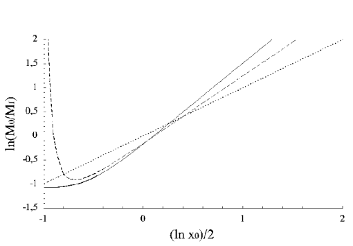
Figure 7: The quantity $\ln(M_{0}/M_{f})$ as a function of $\,\pi/g^{2}-1=(\ln x_{0})/2$, for N=3. Full line: numerical integration; dashed line: leading order relation (from Eq. (57)); long dashed line: approximate integration according to equation (107).

This expression is identical to Eq. (83) that has been used to eliminate the scale dependence in the effective potential. In contrast to the linearized version, Eq. (82), it holds even in cases where $M_{0}\gg M_{f}$, i.e., at weak coupling, where terms involving $\ln(M_{0}/M_{f})$ may become of order $N$; such large logarithms do not enter the $\beta$-function (as we have seen earlier, $\beta^{(1)}$ remains small at weak coupling), but can be generated by the integration over a sufficiently large range of values of $g$ in Eq. (106).

The effective potential that we have obtained does not depend on the scale $M_{0}$ (at order $1/N$) , but the separation of the mass between a contribution coming from the minimum of the potential $M_{min}\sim\langle\bar{\psi}\psi\rangle$ and one coming from the self-energy $\Sigma$ depends on the scale $M_{0}$. In particular, since (see Eqs. (95) and (94))

$$\bar{Z}^{\prime(1)}=2\int{\rm d}g{\gamma^{(1)}(g)\over\beta^{(0)}(g)}\sim\ln{1\over g},$$ (108)

$M_{\Sigma}/M_{f}$ may become of order unity if $g$ is too small (see Eq. (80)); this, however, occurs only for very small $g$, such that $g^{2}\mathrel{\hbox to0.0pt{\raise 2.20013pt\hbox{$<$}\hss}{\lower 2.20013pt\hbox{$\sim$}}}{\rm e}^{-N}$.

Finally let us mention that while the choice of the scale for the effective potential is not an issue at this point (since the effective potential does not depend on $g$), we shall see that at high temperature the coupling constant effectively reappears in the calculation, at a scale determined by the temperature. This will be discussed in subsection V.4.

IV The renormalized effective potential at finite temperature

We turn now to the computation of the effective potential at finite temperature. At leading order in the $1/N$ expansion, the effective potential can be split into a zero temperature contribution and a finite temperature one which is free of ultraviolet divergences. Thus, at leading order, the technical difficulties associated with the elimination of divergences are localized in the contribution which has been studied in the previous section. Beyond leading order however, the situation becomes more complicated and, at some stage of the calculation, ultraviolet divergences appear in terms which depend on the temperature. As mentioned in the introduction, one expects on general grounds LeBellac96 ; Landsman:uw ; Collins84 that such contributions should eventually cancel without the need for counterterms other than those introduced at zero temperature. We shall verify explicitly in this section that this indeed happens.

IV.1 The leading order contribution

At leading order in the $1/N$ expansion, the effective potential is given by the fermionic contribution, i.e., the first two terms in Eq. (25). As we just mentioned, it can be written as the sum of a “zero temperature” contribution, $V^{(0)}(M)$, and a finite temperature one, $\tilde{V}^{(0)}(M,T)$, which vanishes as $T\to 0$. We shall denote the complete bare potential at leading order by $V^{(0)}_{B}(M_{B},T)$, i.e., $V^{(0)}_{B}(M_{B},T)=V^{(0)}_{B}(M_{B})+\tilde{V}^{(0)}_{B}(M_{B},T)$. To isolate the zero temperature contribution, we rewrite the sum over Matsubara frequencies in Eq. (25) as

$$-T\sum_{n,odd}\ln\left(1+{M_{B}^{2}\over\omega_{n}^{2}+p^{2}}\right)=\oint{{\rm d}\omega\over 2\pi i}\,n(\omega)\ln\left(1+{M_{B}^{2}\over-\omega^{2}+p^{2}}\right)$$ (109)

where

$$n(\omega)={1\over{\rm e}^{\beta\omega}+1}$$ (110)

is the fermionic statistical factor, and the integration contour is a set of circles surrounding each of the Matsubara frequencies. By deforming this contour into two lines parallel to the imaginary axis, i.e., by writing $\oint=\int_{-i\infty+\epsilon}^{+i\infty+\epsilon}+\int_{i\infty-\epsilon}^{-i\infty-\epsilon}$, and using the property $n(-\omega)=1-n(\omega)$, one can rewrite the integral as

$$\int_{-i\infty+\epsilon}^{+i\infty+\epsilon}{{\rm d}\omega\over 2\pi i}(1-2n(\omega))\ln\left(1+{M_{B}^{2}\over-\omega^{2}+p^{2}}\right).$$ (111)

The term which does not contain the statistical factor gives the zero temperature contribution and it has been dealt with in subsection III.1. The term with the statistical factor is the finite temperature contribution $\tilde{V}^{(0)}_{B}(M_{B},T)$. It can be calculated by performing a further deformation of the integration contour so as to pick up the singularities on the real $\omega$-axis. We get:

$$\tilde{V}^{(0)}_{B}(M_{B},T)=-{2\over\beta}\int_{0}^{\infty}{{\rm d}p\over\pi}\ln\left(1+{\rm e}^{-\beta E_{p}}\right).$$ (112)

where $E_{p}=\sqrt{p^{2}+M_{B}^{2}}$.

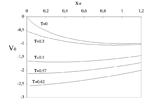
Figure 8: The leading order renormalized potential $V^{(0)}$ (divided by $NM_{f}^{2}/4\pi$) as a function of $x_{M}$, for various temperatures $T$ (in units of the fermion mass $M_{f}$). The temperature $T=0.57M_{f}$ is the temperature $T_{c}$ discussed in the next section (see Eq. (134)), and $0.62M_{f}=1.1T_{c}$.

At this order, the renormalized potential is immediately obtained by substituting $M$ for $M_{B}$ in the equation above. By combining with the zero temperature contribution (55), one obtains then the leading order renormalized effective potential at finite temperature:

$$V^{(0)}(M,T)={M^{2}\over 4\pi}\left(\ln{M^{2}\over M_{f}^{2}}-1\right)-{2\over\beta}\int_{0}^{\infty}{{\rm d}p\over\pi}\ln\left(1+{\rm e}^{-\beta E_{p}}\right).$$ (113)

A noteworthy feature of this expression is that it is analytic around $M=0$, in contrast to the zero temperature contribution. To see that, consider the derivative of $V^{(0)}(M,T)$ with respect to $M^{2}$:

$${\partial V^{(0)}(M,T)\over\partial M^{2}}={1\over 4\pi}\ln{M^{2}\over M_{f}^{2}}+\int_{0}^{\infty}{{\rm d}p\over\pi E_{p}}\,{1\over{\rm e}^{\beta E_{p}}+1}.$$ (114)

The integral in Eq. (114) is infrared divergent when $M\to 0$. By isolating the (logarithmic) singularity one gets Dolan:qd :

$$\int_{0}^{\infty}{{\rm d}p\over E_{p}}\,{1\over{\rm e}^{\beta E_{p}}+1}\approx-{1\over 4}\ln\left({\beta^{2}M^{2}\over\pi^{2}}\right)-{1\over 2}\gamma_{E}+O(\beta^{2}M^{2}),$$ (115)

where $\gamma_{E}$ is Euler’s constant. This formula shows that the logarithms $\sim\ln M^{2}$, at the origin of the non-analyticity, cancel in Eqs. (114) and (113).

As we did in subsection III.1, it is convenient to express the effective potential in terms of the variable $x_{M}=M^{2}/M_{f}^{2}$ (see Eq. (55)). With a slight abuse in the notation, one can then write:

$$V^{(0)}(x_{M},T)={M_{f}^{2}\over 4\pi}\left[x_{M}(\ln x_{M}-1)-{8\over b}\;\int_{0}^{\infty}{\rm d}{\rm u}\ln(1+{\rm e}^{-b\sqrt{u^{2}+x_{M}}})\right],$$ (116)

where $b\equiv M_{f}/T$.

A plot of the leading order effective potential is given in Fig. 8. As seen on this figure, as $T$ increases, the minimum is shifted to lower and lower values of $x_{M}$ and eventually reaches $x_{M}=0$. We come back to this in subsection V.1 when discussing the restoration of chiral symmetry.

IV.2 The $1/N$ contribution and the total effective potential

As was the case already at T=0 (see subsection III.2), at $T\neq 0$ both the fermionic and the bosonic parts in (25) contribute at next-leading-order. The fermionic contribution originates in the next-to-leading order renormalization of $M_{B}$ and $g_{B}$ in $V^{(0)}_{B}(M_{B},T)$. The renormalization of $\tilde{V}^{(0)}_{B}(M_{B},T)$ in Eq. (112) amounts simply to the replacement $M_{B}^{2}\to M^{2}(1+Z^{\prime(1)}/N)$, with $Z^{\prime(1)}$ given by Eq. (72). The resulting expression can be written as $\tilde{V}^{(0)}(M,T)+(1/N)\tilde{V}_{f}^{(1)}(M,T)$, with $\tilde{V}^{0}{(0)}(M,T)$ given by Eq. (112) with $M_{B}\to M$ and

$$\tilde{V}^{(1)}_{f}(M,T)=M^{2}\ln\ln\left({\Lambda\over M_{f}}\right)\left(\int_{0}^{\infty}{{\rm d}k\over\pi}{n_{k}\over E_{k}}\right)+\bar{Z}^{\prime(1)}M^{2}\left(\int_{0}^{\infty}{{\rm d}k\over\pi}{n_{k}\over E_{k}}\right).$$ (117)

where $E_{k}=\sqrt{k^{2}+M^{2}}$ and $n_{k}=n(\omega=E_{k})$ (see Eq. (110)). The first term in Eq. (117) introduces a new divergence, not present at T=0, and which depends explicitly on the temperature. From the discussion at the beginning of this section, such a divergence should not remain in the final result, and indeed we shall see shortly that it is canceled by a similar one coming from the finite temperature contribution of the bosonic part, to which we now turn.

The bosonic contribution comes from the last term of Eq. (25):

$$V^{(1)}_{b,B}(M_{B},T)={1\over 2}\int[d^{2}Q]\ln\left[1+g_{B}^{2}\Pi(\omega,q;M_{B},T,\Lambda)\right].$$ (118)

It is convenient to write the sum over Matsubara frequencies in Eq. (118) as a contour integral, as we did for the fermionic contribution in Eq. (109). By exploiting the parity property $\Pi(-\omega,q)=\Pi(\omega,q)$, one can then write:

$$V^{(1)}_{b,B}(M_{B},T)={1\over 2}\int{{\rm d}q\over 2\pi}\int_{-i\infty+\epsilon}^{i\infty+\epsilon}\,{{\rm d}\omega\over 2\pi i}\,(1+2N(\omega))\,\ln\left[1+g_{B}^{2}\Pi(\omega,q;M_{B},T,\Lambda)\right],$$ (119)

where

$$N(\omega)={1\over{\rm e}^{\beta\omega}-1}$$ (120)

is the bosonic statistical factor.

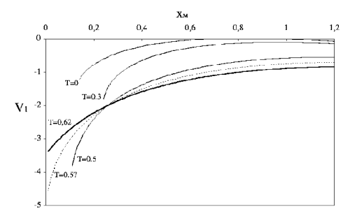
Figure 9: The next-to-leading order renormalized potential $V^{(1)}$ (divided by $M_{f}^{2}/4\pi$) as a function of $x_{M}>x_{M_{*}}(T)$, for various temperatures $T$ (in units of the fermion mass $M_{f}$). The temperature $T=0.57M_{f}$ is the temperature $T_{c}$ discussed in the next section (see Eq.134)), and $0.62M_{f}=1.1T_{c}$.

The expression (119) of the bosonic part of the effective potential is analogous to the corresponding one for the fermionic part, Eq.(111). However in contrast to what happened in the fermionic case where Eq.(111) leads naturally to a separation between zero temperature and non-zero temperature contributions, this is not quite so here: the term containing the statistical factor $N(\omega)$ certainly vanishes as $T\to 0$, and as such can be considered as a genuine finite temperature contribution; the term without the statistical factor reduces to the zero temperature effective potential as $T\to 0$, but it does contain finite temperature contributions (since $\Pi$ depends now on $T$). Nevertheless, the separation suggested by Eq.(119) is useful as it allows us to clearly isolate the ultraviolet divergences: these are contained entirely in the term without the statistical factor. We shall then add the zero temperature counterterms (64) to that term, renormalize the mass and the coupling constant with the leading order renormalization constants ($Z^{(0)}$ from Eq. (51) and $Z^{\prime(0)}=1$), and rewrite the renormalized effective potential $V^{(1)}_{b}(M,T)$ as the sum of two contributions: $V^{(1)}_{b}(M,T)=V^{(1)}_{b,1}(M,T)+V^{(1)}_{b,2}(M,T)$ with

$$V^{(1)}_{b,1}(M,T)={1\over 2}\int^{\Lambda}{{\rm d}^{2}q\over(2\pi)^{2}}\ln\left[{D^{-1}(iq_{0},q;M,T)\over D_{0}^{-1}(Q_{E};M_{f})}\right]+{M_{f}^{2}\over 4\pi}\ln{\Lambda^{2}\over M_{f}^{2}}\,+{M_{f}^{2}\over 4\pi}\ln\ln{\Lambda\over M_{f}},$$ (121)

$$V^{(1)}_{b,2}(M,T)=\int_{-\infty}^{+\infty}{{\rm d}q\over 2\pi}\int_{-i\infty+\epsilon}^{i\infty+\epsilon}{{\rm d}\omega\over 2\pi i}\,N(\omega)\,\ln\left[D^{-1}(\omega,q;M,T)\right],$$ (122)

where $D^{-1}(iq_{0},q;M,T)\equiv D_{0}^{-1}(Q_{E};M)+g^{2}\tilde{\Pi}(iq_{0},q;M,T)$ is the renormalized inverse $\sigma$-propagator studied in App. A.

Clearly, when $T\to 0$, $V^{(1)}_{b,1}(M,T)$ becomes the zero temperature part of the bosonic contribution to the potential analyzed in subsection III.2; in the same limit $V^{(1)}_{b,2}(M,T)$ vanishes. The divergent contributions to $V^{(1)}_{b,1}(M,T=0)$ are dealt with as in subsection III.2. When the temperature is non zero, a new divergence occurs in $V^{(1)}_{b,1}(M,T)$. This can be isolated with the help of the asymptotic behaviors of $D_{0}^{-1}$ and $\tilde{\Pi}$ given in App. A (Eqs. (198) and (216), respectively). One gets:

$$V^{(1)}_{b,1}(M,T)\sim-M^{2}\ln\ln\left({\Lambda\over M}\right)\left(\int_{0}^{\infty}{{\rm d}k\over\pi}{n_{k}\over E_{k}}\right).$$ (123)

This divergence cancels that of the renormalized fermionic contribution $\tilde{V}^{(1)}_{f}$ of Eq. (117), as anticipated (the two $\Lambda$-dependent terms in Eqs. (117) and (123) are identical to within terms which vanish as $\Lambda\to\infty$).

At this point, it is useful to go one step further and, in analogy with what we did in Eq. (85) of the previous section, we absorb the finite part of the counterterm into the redefinition of the variable $x_{M}$ according to Eq. (86). Adding $\tilde{V}^{(0)}(M,T)$ and the second term in Eq. (117) one can write (discarding terms of order $1/N^{2}$):

$$\!\!-{2\over\beta}\int_{0}^{\infty}{{\rm d}{\rm k}\over\pi}\ln\left(1+{\rm e}^{-\beta E_{\rm k}}\right)\!+\!{{\bar{Z}^{\prime(1)}}\over N}\,M^{2}\!\int_{0}^{\infty}{{\rm d}{\rm k}\over\pi}{n_{\rm k}\over E_{\rm k}}=-{2M^{2}_{f}\over b}\!\int_{0}^{\infty}{{\rm d}{\rm u}\over\pi}\ln\left(1+{\rm e}^{-b\sqrt{u^{2}+x_{M}}}\right)$$ (124)

with $x_{M}=M^{2}/M_{f}^{2}\;(1+\bar{Z}^{\prime(1)}/N)$, as defined in Eq. (86), and $b=M_{f}/T$. Thus, in complete analogy with the zero temperature case (see Eq. (87)), after the redefinition of the variable $x_{M}$, the leading order contribution to the renormalized potential keeps the form of $V^{(0)}(x_{M},T)$ given by Eq. (116).

By using the results just obtained and defining new functions $F(x_{M},T)$, and $G(x_{M},T)$, we can then write the complete effective potential at order $1/N$ in the form:

$$V(x_{M},T) = {M_{f}^{2}\over 4\pi}\left[Nx_{M}(\ln x_{M}-1)-N\;{8\over b}\;\int_{0}^{\infty}{\rm d}{\rm u}\ln(1+{\rm e}^{-b\sqrt{u^{2}+x_{M}}})\right.$$ (125)

$$\qquad\qquad\qquad\qquad+\xi(x_{M}-1)+F(x_{M},T)+G(x_{M},T)\Big{]},$$

where the functions $F$ and $G$ are given in App. B. The function $F(x,T)$ is an extension at finite temperature of the function $F_{0}(x)$ introduced in the previous section; to within an additive constant, it is proportional to the finite part of $V^{(1)}_{b,1}(M,T)$. The function $G(x,T)$ is proportional to $V^{(1)}_{b,2}(M,T)$:

$$V^{(1)}_{b,2}={M^{2}_{f}\over 4\pi}G(x_{M},T).$$ (126)

It can be calculated by deforming the integration contour so that it goes around the singularities on the real axis. This operation requires that grand circles at infinity generate no contribution, and that the discontinuity of the integrand vanishes at $\omega=0$, properties that are both satisfied. The resulting integral along the cut is then finite because of the statistical factor. It can be written as:

$$V^{(1)}_{b,2}(M) = \int_{-\infty}^{+\infty}{{\rm d}q\over 2\pi}\int_{0}^{\infty}{{\rm d}\omega\over 2\pi\,i}\,N(\omega)\,\ln\left[{D^{-1}(\omega+i\epsilon,q;M,T)\over D^{-1}(\omega-i\epsilon,q;M,T)}\right]\,$$ (127)

$$= \int_{-\infty}^{+\infty}{{\rm d}q\over 2\pi}\int_{0}^{\infty}{{\rm d}\omega\over 2\pi}\,N(\omega)\,2\,{\rm Im}\ln D^{-1}(\omega+i\epsilon,q;M,T).$$

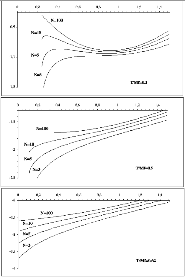
Figure 10: The effective potential (divided by $NM_{f}^{2}/4\pi$) as a function of $x_{M}>x_{M_{*}}(T)$, for various values of $N$ and the temperature $T$. The temperature $T=0.57M_{f}$ is the temperature $T_{c}$ discussed in the next section (see Eq.134)), and $0.62M_{f}=1.1T_{c}$.

One may also express the argument of the logarithm in terms of the phase shift $\delta$ of quark-quark scattering (see e.g. Eq. (232)):

$${\rm e}^{-2i\delta}={D^{-1}(\omega+i\epsilon,q;M,T)\over D^{-1}(\omega-i\epsilon,q;M,T)},$$ (128)

with

$$\tan\delta(\omega,q;M,T)=-g^{2}{{\rm Im}\Pi(\omega+i\epsilon,q;M,T)\over{\rm Re}D^{-1}(\omega+i\epsilon,q;M,T)}.$$ (129)

The latter are the expressions we use to calculate the function $G(x_{M},T)$ numerically and to understand its behavior for small values of $x_{M}$ (see App. B).

To get an intuitive picture for what these formulae represent, let us first rewrite the expression (127) by integrating by parts,

$$V^{(1)}_{b,2}(M,T)=\int_{-\infty}^{+\infty}{{\rm d}q\over 2\pi}\int_{0}^{\infty}{{\rm d}\omega\over\pi}\,{1\over\beta}\ln\left(1-{\rm e}^{-\beta\omega}\right){{\rm d}\delta\over{\rm d}\omega}.$$ (130)

(The boundary term does not contribute because $\delta(\omega,q)$ vanishes at small $\omega$ in the same way as ${\rm Im}\Pi(\omega,q)$.) Then, let us imagine that the $\sigma$ excitation corresponds to a simple pole of the propagator, i.e., assume $D^{-1}(\omega,q)=\omega^{2}-\omega_{q}^{2}$. In this case, ${\rm d}\delta/{\rm d}\omega=\pi\delta(\omega-\omega_{q})$, and $V^{(1)}_{b,2}(M)$ is simply

$$V^{(1)}_{b,2}(M)={1\over\beta}\int_{-\infty}^{+\infty}{{\rm d}q\over 2\pi}\ln\left(1-{\rm e}^{-\beta\omega_{q}}\right),$$ (131)

which is the free energy density of noninterating bosons with energies $\omega_{q}$. In the present case however, the sigma excitation does not correspond to a pole of the propagator (see subsection V.2), and this simple picture does not quite hold.

The $1/N$ contribution to the renormalized effective potential given by the second line in Eq. (125) is displayed in Fig. 9. As was the case at zero temperature (see the remark at the end of subsection III.2)), there is a minimum value $x_{M_{*}}(T)$ of $x_{M}$ below which a Landau pole appears and the function $F(x_{M},T)$ becomes complex. For this reason, the next-to-leading order contribution to the potential is plotted in Fig. 9 only for $x_{M}>x_{M_{*}}(T)$ (the way $x_{M_{*}}$ depends on the temperature is discussed in subsection V.2). In the same region $x_{M}<x_{M_{*}}(T)$ where $F$ is not real, the function $G$ takes anomalously large and negative values (see Fig. 19 and the discussion in App. B). For $x_{M}\mathrel{\hbox to0.0pt{\raise 2.20013pt\hbox{$>$}\hss}{\lower 2.20013pt\hbox{$\sim$}}}x_{M_{*}}$, both $G(x_{M},T)$ and $F(x_{M},T)$, and therefore also $V_{1}(x_{M})$, have a large slope as can be seen in Fig. 9.

The complete effective potential is displayed in Fig. 10 for various values of $N$ and the temperature $T$, as a function of $x_{M}$ (for $x_{M}>x_{M_{*}}(T)$). The curves labelled $N=100$ are very close to those corresponding to the leading order potential (not drawn). If we follow these curves, one recovers the behavior of the leading order potential, already discussed: as the temperature increases, the minimum of the potential shifts to lower values of $x_{M}$ and becomes more and more shallow, until it reaches $x_{M}=0$ where it becomes again a pronounced minimum. A striking feature of the curves in Fig. 10 is the large effect of the $1/N$ corrections: already at moderate temperatures, one sees that the minimum disappears for small values of $N$. This is to be related to the large slopes at small $x_{M}$ of the curves in Fig. 9, which drive quickly the minimum to low values of $x_{M}$, making this minimum dangerously close to the threshold $x_{M_{*}}$ for the appearance of the Landau pole. Note however that, at larger temperatures, the potential has a well defined minimum at $x_{M}=0$ for all values of $N$.

All these properties of the effective potential, and their physical interpretation, will be discussed at length in the next section.

V Thermodynamics

We use now the results that have been established in the previous sections to discuss the thermodynamical properties of the system. We start, in the next subsection, by reviewing known leading order results concerning the restoration of chiral symmetry at a finite temperature $T_{c}$. In this one-dimensional system, this phenomenon is specific of the mean field, or large $N$, approximation based on uniform quark condensates, i.e., on constant solutions of the gap equation (15). (As argued in Ref. Dashen:xz , kink configurations of the condensate, if taken into account, would presumably prevent chiral symmetry breaking at any non-zero temperature). At next-to-leading order in the $1/N$ expansion the fluctuations around the uniform condensate provide a small correction to the mean field picture as long as the temperature remains small. But as the temperature increases these fluctuations become large, eventually making the behavior of the system pathological; as we shall see in subsection V.3, this results in a breakdown of the $1/N$ expansion at some temperature below the mean field transition temperature $T_{c}$. We shall see that this breakdown is related to the presence of a Landau pole which is discussed in subsection V.2.

The last two subsections are devoted to the high temperature limit ($T\gg T_{c}$). There chiral symmetry is realized, and the $1/N$ expansion remains a good approximation scheme. It provides a description of the system as weakly interacting fermions, as expected from asymptotic freedom. Quite remarkably, while the effective potential obtained in the previous section does not depend explicitly on the coupling constant, we shall see that the pressure can nevertheless be expanded in terms of an effective coupling whose magnitude decreases logarithmically with the temperature. To better understand this result, a direct perturbative calculation of the pressure is presented in the last subsection.

V.1 Restoration of chiral symmetry in leading order

The finite temperature effective potential at leading order may be written (see Eq. (116)):

$$V^{(0)}(M,T)={M^{2}\over 4\pi}\left(\ln{M^{2}\over M_{f}^{2}}-1\right)-{2\over\pi\beta}\int_{0}^{\infty}{\rm d}k\ln\left(1+{\rm e}^{-\beta E_{k}}\right),$$ (132)

with $E_{k}=\sqrt{k^{2}+M^{2}}$. As discussed in subsection IIC, at this order the minimum of Eq. (132) is simply the quark mass $M_{f}(T)$. It is a decreasing function of $T$. A simple analysis shows that, at small $T$, this decrease is exponentially small:

$${M_{f}(T)-M_{f}\over M_{f}}\approx\sqrt{{2\pi T\over M_{f}}}\,{\rm e}^{-M_{f}/T}.$$ (133)

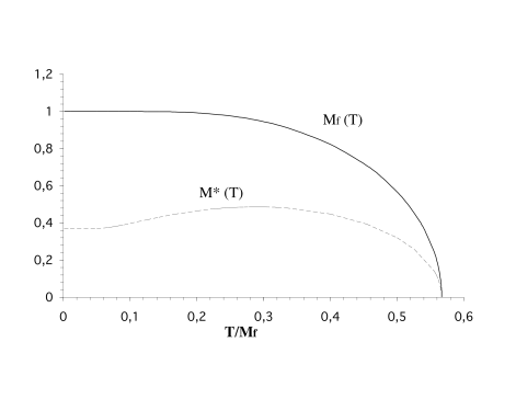
Figure 11: The fermion mass $M_{f}(T)$ in leading order in the $1/N$ expansion as a function of $T/M_{f}$. Also indicated is the value $M_{*}(T)$ of $M$ below which a Landau pole appears (see subsection V.2 and App. A).

As the temperature increases further, however, $M_{f}(T)$ becomes smaller and smaller and eventually vanishes, as can be seen from the plot in Fig. 11 which displays the function $M_{f}(T)$ obtained numerically. One may use the expansion in Eq. (115) to calculate the temperature $T_{c}$ at which $M_{f}(T)$ vanishes Jacobs:ys ; Harrington:tf . One gets:

$$T_{c}=M_{f}{{\rm e}^{\gamma_{E}}\over\pi}\simeq 0.567M_{f}.$$ (134)

As $T\to T_{c}$ the system undergoes a second order phase transition with mean field exponents. To verify this explicitly, we expand the effective potential around $M=0$:

$$V^{(0)}(M,T)\simeq V^{(0)}(0,T)+a\left({M\over M_{f}}\right)^{2}+b\left({M\over M_{f}}\right)^{4}$$ (135)

with

$$a={M_{f}^{2}\over 2\pi}\ln\left({T\over T_{c}}\right)\qquad\qquad b={7\zeta(3)M_{f}^{4}\over 32\pi^{3}T^{2}}$$ (136)

where $\zeta(3)\approx 1.202$. The coefficient $a$ follows easily form the expansion (115). The coefficient $b$ is obtained by using the expression (109) of the potential as a sum over the Matsubara frequencies. By taking the second derivative of this expression with respect to $M^{2}$ one obtains a convergent sum which is proportional to $b$:

$${T\over 4}\sum_{n}{1\over[|2n+1|\pi T]^{3}}={7\zeta(3)\over 16\pi^{3}T^{2}}={2b\over M_{f}^{4}}.$$ (137)

(Note that the expansion (135) of the potential is meaningful only at finite temperature, as is obvious on the form of the coefficients $a$ and $b$ which are singular in the limit $T\to 0$.) The form (135) of the effective potential controls the behavior of $M_{f}(T)/M_{f}$ in the vicinity of $T_{c}$. A simple calculation gives:

$${M_{f}(T)\over M_{f}}\sim\sqrt{{-a\over 2b}}\simeq\sqrt{{8\pi^{2}\over 7\zeta(3)}}{T_{c}\over M_{f}}\sqrt{{T_{c}-T\over T_{c}}}.$$ (138)

Above $T_{c}$, the fermion mass $M_{f}(T)$ vanishes, and so does the (renormalized) quark condensate: $\langle\bar{\psi}\psi\rangle=-NM_{f}(T)/g^{2}$ (see Eq. (29)). Thus, at $T_{c}$ the discrete chiral symmetry is restored.

The pressure is simply related to the effective potential at its minimum: $P(T)=NP^{(0)}=-NV^{(0)}(M=M_{f}(T),T)$. The entropy density can be easily calculated from $s(T)={{\rm d}P}/{{\rm d}T}$. Since $V^{(0)}(M,T)$ is stationary for variations of $M$ around the value $M=M_{f}(T)$, the derivative can be simply taken at fixed $M$. The result is that the entropy density is just that of free particles of mass $M_{f}(T)$:

$$s(T)=Ns^{(0)}(T)=-2N\int_{-\infty}^{\infty}{dk\over 2\pi}\left[(1-n_{k})\ln(1-n_{k})-n_{k}\ln n_{k}\right],$$ (139)

where $n_{k}=n(E_{k})$ is the fermion statistical factor (see Eq. (110)), and $E_{k}=\sqrt{k^{2}+M_{f}^{2}(T)}$. When $T>T_{c}$, the fermion mass vanishes and we have ($\int_{0}^{\infty}dx\ln(1+{\rm e}^{-x})=\pi^{2}/12$):

$$P^{(0)}={\pi T^{2}\over 6}\qquad\qquad s^{(0)}={{\rm d}P^{(0)}\over{\rm d}T}={\pi T\over 3}.$$ (140)

Thus for $T>T_{c}$, interaction effects completely disappear, and the system behaves as a system of free massless fermions.

We show in the last two subsections that the $1/N$ corrections do not alter much this picture at high temperature where, due to asymptotic freedom, the effect of the interactions remains small. But the $1/N$ corrections do affect very strongly the behavior of the system below $T_{c}$, as we shall see shortly. Before turning to these $1/N$ corrections, we shall, in the next subsection, continue to discuss physical properties of the system in the mean field approximation; some of these will be useful in the interpretation of the next-to-leading order results.

V.2 The $\sigma$ excitation and quark-quark scattering amplitude

At zero temperature, the propagator $D_{0}(Q;M_{f})$, obtained by setting $M=M_{f}$ in Eq. (196), describes $\sigma$-meson excitations with mass $M_{\sigma}=2M_{f}$. This is easily seen by solving the equation $D_{0}^{-1}(Q_{E}^{2}=-M_{\sigma}^{2};M_{f})=0$ for $M_{\sigma}$. Note however that this point where $D_{0}^{-1}$ vanishes does not correspond to a simple pole in the $\sigma$ propagator, but to a branch point limiting the region of phase space where the $\sigma$ excitation can decay into quark-antiquark pairs.

Figure 12: The real part of $D_{0}^{-1}(\omega,q;M)$ as a function of $(\omega^{2}-q^{2})/M^{2}$ for $M<M_{f}$. For $M=M_{f}$, ${\rm Re}D_{0}^{-1}$ vanishes at the single point $(\omega^{2}-q^{2})/M_{f}^{2}=4$, beyond which the imaginary part starts to grow. For an arbitrary $M$, Re$D_{0}^{-1}(\omega,q;M)$ has a minimum at this point, with value $(g^{2}/\pi)\ln(M/M_{f})$ (see App. A). When $M=M_{*}=M_{f}/e$, Re $D_{0}^{-1}$ vanishes at $\omega^{2}=q^{2}$.

In order to see that we need to perform an analytic continuation from the Euclidean momentum $Q_{E}=(q_{0},q)$ to the Minkowski one $Q_{M}=(\omega,q)$, with $q_{0}\to-i\omega$. From Eq. (196), one gets:

$$D^{-1}_{0}(\omega,q;M)={g^{2}\over 2\pi}\left[\ln\left({M^{2}\over M_{f}^{2}}\right)+B_{0}\left({-\omega^{2}+q^{2}\over M^{2}}\right)\right].$$ (141)

Let us set $\omega_{q}=\sqrt{q^{2}+4M_{f}^{2}}$. The inverse propagator $D^{-1}_{0}(\omega,q;M_{f})$ has cuts on the real $\omega$ axis for $\omega>\omega_{q}$ and $\omega<-\omega_{q}$; the corresponding imaginary part is (for $\omega>0$):

$${\rm Im}D^{-1}_{0}(\omega+i\epsilon,q;M_{f})=-{g^{2}\over 2}\sqrt{{\omega^{2}-\omega_{q}^{2}\over\omega^{2}-q^{2}}}\,\Theta(\omega-\omega_{q}).$$ (142)

The point $\omega=\omega_{q}$, is the branch point corresponding to the threshold mentioned above. A plot of ${\rm Re}D_{0}^{-1}(\omega+i\epsilon,q;M)={\rm Re}D_{0}^{-1}(\omega+i\epsilon,q;M_{f})+(g^{2}/\pi)\ln(M/M_{f})$ is displayed in Fig. (12).

At finite temperature the threshold remains located at $2M_{f}(T)$, as long as $T<T_{c}$. To see that, consider the equation which defines $M_{\sigma}$;

$$D^{-1}(\omega=M_{\sigma},q=0;M_{f}(T))=0,$$ (143)

where $D^{-1}=D_{0}^{-1}+g^{2}\tilde{\Pi}$ is the finite temperature $\sigma$ propagator studied in App. A. Let us set $M_{\sigma}=2M_{f}(T)$ and verify that indeed this is the solution. Using the explicit expressions for $\tilde{\Pi}(\omega,q)$ given in App. A, we get:

$$D^{-1}(\omega=M_{\sigma},q=0;M_{f}(T))={g^{2}\over\pi}\ln\left({M_{f}(T)\over M_{f}}\right)+2g^{2}\int_{0}^{\infty}{{\rm d}k\over\pi}{n_{k}\over E_{k}}=0,$$ (144)

with $n_{k}$ as in Eq. (139) above. This equation is precisely that which determines $M_{f}(T)$, i.e., the gap equation obtained by equating the right hand side of Eq. (114) to zero, which proves the point.

A more complete description of the $\sigma$ excitation is obtained from the corresponding spectral function $\rho(\omega,q)$. At zero temperature, we define ($\omega$ real):

$$\rho_{0}(\omega,q)={1\over i}[D_{0}(\omega+i\epsilon,q;M_{f})-D_{0}(\omega-i\epsilon,q;M_{f})]=2{\rm Im}D_{0}(\omega+i\epsilon,q;M_{f}).$$ (145)

This is an odd function of $\omega$. Using the formulae given above, one easily obtains (for $\omega>0$):

$$\rho_{0}(\omega,q)={4\over g^{2}}\sqrt{{\omega^{2}-q^{2}\over\omega^{2}-\omega_{q}^{2}}}{\Theta(\omega-\omega_{q})\over 1+{4\over\pi^{2}}\left({\rm Arctanh}\sqrt{{\omega^{2}-\omega_{q}^{2}\over\omega^{2}-q^{2}}}\right)^{2}}.$$ (146)

At fixed $q$, this is a decreasing function of $\omega$, peaked at $\omega\simeq\omega_{q}$; when $\omega\to\infty$, $\rho_{0}(\omega,q)$ vanishes as $\rho_{0}(\omega,q)\sim 4\pi^{2}/(g\ln\omega^{2})^{2}$. By replacing, in Eq. (145), $D_{0}$ by the finite temperature propagator $D(\omega,q;M_{f}(T))$, one obtains the spectral function at finite temperature $\rho(\omega,q;T)$. The typical behavior of $\rho(\omega,q;T)$ for temperatures below and above $T_{c}$ is displayed in Fig. 13. We note, below $T_{c}$, the threshold at $\omega=\sqrt{q^{2}+4M_{f}(T)^{2}}$, beyond which the spectral function resembles $\rho_{0}(\omega,q)$ given by Eq. (146). For $0<\omega<q$, a typical finite temperature contribution appears, that of the scattering of quark-antiquark pairs on quarks or antiquarks present in the heat bath (see App. A for more details). As $T$ approaches $T_{c}$ from below, $M_{f}(T)\to 0$, and the two contributions merge, leaving a sharp peak at small $\omega$. The peak structure survives just above $T_{c}$ (see the curve labelled $T=0.6$ in Fig. 13), but as one raises the temperature the spectral weight becomes spread over a larger and larger energy range, as can be seen in Fig. 13. The behavior of the spectral function is then governed by the high temperature regime of the fermion loop discussed in App. A. In this regime and for large values of $q$ ($q\gg T_{c}$), the spectral function becomes a step function at $\omega=q$ followed by a long logarithmic tail.

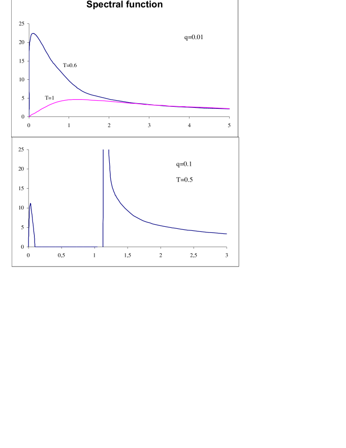
Figure 13: The spectral function of the $\sigma$ excitation above $T_{c}$ (top, $q=0.01$) and below $T_{c}$ (bottom, $q=0.1$), as a function of $\omega$ expressed in units of $M_{f}$ (upper curves) or $M_{f}(T)$ lower curves.

Consider finally the quark-quark scattering amplitude ${\cal T}(\omega,q;M,T)$, where the mass $M$ is treated as an independent parameter. This is the generalization at finite temperature of the quantity introduced in Eq. (62), i.e.: ${\cal T}(\omega,q;M,T)=g^{2}D(\omega,q;M,T).$ At zero momentum, we have (see Eqs. (27)):

$${\cal T}(0,0;M,T)=g^{2}\lim_{q\to 0}D(0,q;M)=\left({{\rm d}^{2}V^{(0)}(M,T)\over{\rm d}M^{2}}\right)^{-1},$$ (147)

This relation may be verified by calculating the second derivative from the expression (113) of the potential and using the results given in App. A to obtain:

$$\lim_{q\to 0}{1\over{\cal T}(0,q;M,T)}={1\over\pi}\left(1+\ln{M\over M_{f}}\right)+2\int_{0}^{\infty}{{\rm d}k\over\pi}\left({M^{2}\over E_{k}^{2}}{{\rm d}n\over{\rm d}E_{k}}+{k^{2}\over E_{k}^{2}}{n\over E_{k}}\right).$$ (148)

The second term in the r.h.s. of Eq. (148) is $\lim_{q\to 0}\tilde{\Pi}(0,q;M,T)$ (where we have used Eq. (199)). The two terms in the integral correspond respectively to the contributions of scattering processes and pair creations (see App. A). As mentioned already, at finite temperature, and when $M\neq 0$, the double limit $\omega\to 0,q\to 0$ of $D(\omega,q)$ is not regular and the result depends on the order in which the two limits are taken. If the limit $q\to 0$ had been taken first, the scattering term, proportional to ${\rm d}n/{\rm d}E$, would be absent in Eq. (148), as may be seen from Eq. (199).

When $M\to 0$, the scattering term vanishes and the limit $\omega\to 0,q\to 0$ of ${\cal T}(\omega,q)$ becomes regular. In that same limit where $M\to 0$, the second term in the integral of Eq. (148) (i.e., the pair creation term) develops a logarithmic divergence, which in fact cancels the logarithm of the $T=0$ contribution (the first term of Eq. (148)). Thus one has (see Eq. (209)):

$$\lim_{M\to 0}{\cal T}(0,0;M,T)={\pi\over\ln(T/T_{c})},$$ (149)

which is nothing but the square of the renormalized coupling constant evaluated at a scale $M_{0}\sim T$ (see Eq. (57)). Thus at high temperature, i.e., when $T\gg T_{c}$, the scattering amplitude becomes small, as expected from asymptotic freedom. It can be also verified that no Landau pole occurs in this regime.

Below $T_{c}$ the situation is complicated by the presence of a Landau pole in the $\sigma$ propagator. The threshold $M_{*}(T)$ for the appearance of the Landau pole, which coincides with the value of $M$ at which the second derivative of $V^{(0)}$ vanishes, is plotted as a function of the temperature in Fig. 11. As the temperature increases, $M_{*}$ is shifted first to slightly larger values: this is because at moderate temperatures the finite temperature contribution in Eq. (148) is dominated by the first, negative, term in the integral. For temperatures beyond approximately $T_{c}/2$ however the second, positive, contribution becomes dominant, resulting in a shift of $M_{*}$ to lower and lower values, reaching $M_{*}=0$ at $T_{c}$. That $M_{*}$ vanishes precisely at $T_{c}$ follows from the simple fact that $M_{*}$ is located between two extrema of the potential, which merge at $T_{c}$. Thus, as $T$ approaches $T_{c}$, the fermion mass $M_{f}(T)$ becomes close to $M_{*}(T)$, and the calculation of the next-to-leading contribution to the effective potential becomes ill defined in the vicinity of its minimum: in particular $F(x_{M};T)$ becomes complex for $x_{M}<x_{M_{*}}$ ($x_{M_{*}}=(M_{*}/M_{f})^{2}$) and both $F(x_{M};T)$ and $G(x_{M};T)$ present large negative slopes for $x_{M}\mathrel{\hbox to0.0pt{\raise 2.20013pt\hbox{$>$}\hss}{\lower 2.20013pt\hbox{$\sim$}}}x_{M_{*}}$ (see discussion in subsection IV.2 and App. B). The latter has important consequences which will become clear in the next subsection.

V.3 The quark condensate at order 1/N

In this subsection, we examine how the physics of chiral symmetry breaking and its restoration, which we have just discussed, is modified by the $1/N$ corrections. Chiral symmetry breaking is characterized by a non-vanishing value of the quark-condensate, and the latter is proportional to the value $M_{min}$ of the minimum of the effective potential (see Eq. (29)). The effective potential has been obtained in subsection IV.2 to order $1/N$ in terms of the renormalization group invariant $x_{M}$ defined in Eq. (86). We shall analyze here the variation with the temperature of $x_{min}\equiv x_{M_{min}}\propto M_{min}^{2}$ obtained at next-to-leading-order.

The quantity $x_{min}(T)$ may be determined to accuracy $1/N$ by following the strategy exposed in subsection II B. Generalizing Eq. (88) at finite temperature, we set

$$x_{min}(T)=x_{min}^{(0)}(T)+{1\over N}x_{min}^{(1)}(T),$$ (150)

where $x_{min}^{(0)}(T)$ is the minimum of $V^{(0)}(x_{M},T)$ in Eq. (116). Clearly, $x_{min}^{(0)}(T)M_{f}^{2}=M_{f}^{2}(T)$, where $M_{f}(T)$ is the temperature dependent quark mass introduced in subsection V.1, and plotted in Fig. 11. The correction $x_{min}^{(1)}(T)$ is given by (see Eq. (88)):

$$x_{min}^{(1)}=-{\left.{{\rm d}V^{(1)}(x_{M},T)\over{\rm d}x_{M}}\right|_{x_{min}^{(0)}(T)}\over\left.{{\rm d}^{2}V^{(0)}(x_{M},T)\over{\rm d}x_{M}^{2}}\right|_{x_{min}^{(0)}(T)}},$$ (151)

with

$${{\rm d}V^{(1)}(x_{M},T)\over{\rm d}x_{M}}=\xi+F^{\prime}({x_{min}^{(0)}(T)},T)+G^{\prime}({x_{min}^{(0)}(T)},T),$$ (152)

and ${{\rm d}^{2}V^{(0)}(x_{M},T)}/{{\rm d}x_{M}^{2}}$ can be determined from the results of subsection V.1. In Eq. (152), $F^{\prime}$ and $G^{\prime}$ are the derivatives of the functions $F$ and $G$ with respect to $x_{M}$; they are calculated numerically.

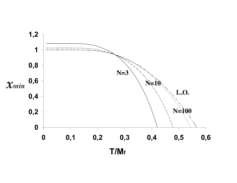
Figure 14: The value of $x_{min}$ calculated from Eqs. (150) and (151), as a function of the temperature $T$ (in units of $M_{f}$), and for various values of $N$. The curve labelled L.O. corresponds to the leading order potential.

A plot of $x_{min}(T)$ is given in Fig. 14. At small $T$, $x_{min}>1$, in agreement with the study of the effective potential at zero temperature (see the caption of Fig. 6). However, when the temperature $T$ increases, the $1/N$ correction eventually turns negative at $T\sim T_{c}/2$ and becomes large when the temperature increases further. Thus, for instance, $|x_{min}^{(1)}/x_{min}^{(0)}|\simeq 0.1$ when $T/T_{c}\sim 0.55$, $|x_{min}^{(1)}/x_{min}^{(0)}|\simeq 1$ when $T/T_{c}\sim 0.65$, $|x_{min}^{(1)}/x_{min}^{(0)}|\simeq 10$ when $T/T_{c}\sim 0.85$ and $|x_{min}^{(1)}/x_{min}^{(0)}|\simeq 30$ when $T/T_{c}\sim 0.92$. Thus, when $T/T_{c}\mathrel{\hbox to0.0pt{\raise 2.20013pt\hbox{$>$}\hss}{\lower 2.20013pt\hbox{$\sim$}}}0.65$ the $1/N$ correction becomes too large to be really considered as a “correction”, and the $1/N$ expansion breaks down. This is to be contrasted with the situation at zero temperature where $|x_{min}^{(1)}/x_{min}^{(0)}|\simeq 0.25$ (see Eq. (88) and the discussion after). Note that what makes $|x_{min}^{(1)}/x_{min}^{(0)}|$ large as $T$ approaches $T_{c}$ is the numerator ${\rm d}V^{(1)}/{\rm d}x_{M}$ (the denominator ${\rm d}^{2}V^{(0)}/{\rm d}x_{M}^{2}$ goes to a constant as $T\to T_{c}$); as we have already discussed, both $F^{\prime}(x_{M})$ and $G^{\prime}(x_{M})$ become large and negative as $x_{M}$ approaches $x_{M_{*}}$, and $x_{min}$ does approach $x_{M_{*}}$ as the temperature increases.

This pathological result is confirmed by a direct (numerical) minimization of the potential in Eq. (125). For all values of $N$ and $T$, one finds values of $x_{min}(T)$ very close to those deduced from Eqs. (150)-(151) whenever the minimum exists (the two evaluations of $x_{min}(T)$ may differ a priori by terms of order $1/N^{2}$). However, as anticipated in subsection IV.2, the potential no longer has a minimum when $T$ exceeds a certain value, which depends on $N$: for $N=100$, the minimum ceases to exist when $T\geq 0.93T_{c}$, for $N=10$ when $T\geq 0.63T_{c}$ and for $N=3$ when $T\geq 0.51T_{c}$. Again the disappearance of the minimum may be related to the rapid drop of the functions $F(x_{M},T)$ and $G(x_{M},T)$ in the vicinity of $x_{M_{*}}$, the value of $x_{M}$ below which a Landau pole appears, as discussed in App. B.

At this point one could speculate and try to relate the breakdown of the $1/N$ expansion to the fact that the true transition temperature of the model is presumably $T_{c}=0$ Dashen:xz . The mean field approximation which ignores part of the important degrees of freedom (e.g. the kink configurations) gives a poor representation of the physics of the system at finite temperature. This mean field physics persists for moderate temperatures: then the fluctuations around the uniform condensate do not change significantly the state of the system. But beyond some value of the temperature the fluctuations become dominant and perhaps mimic the effect of degrees of freedom left-out in the mean field approximation: these fluctuations are responsible for the rapid decrease of $x_{min}$ for $T\mathrel{\hbox to0.0pt{\raise 2.20013pt\hbox{$>$}\hss}{\lower 2.20013pt\hbox{$\sim$}}}T_{c}/2$ which drives the system towards its true equilibrium state, where chiral symmetry is restored.

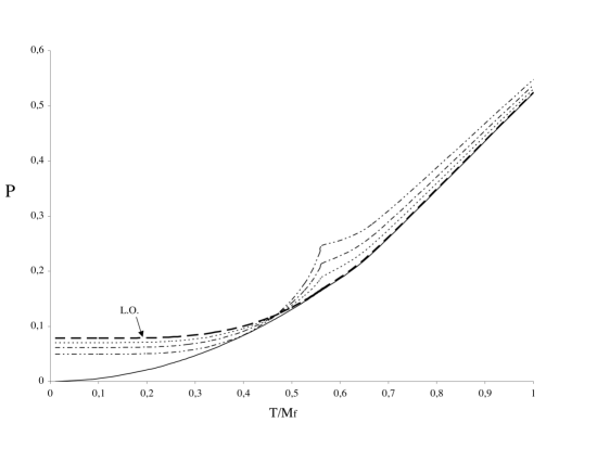
Figure 15: The pressure as a function of $T/M_{f}$. The full line is the pressure of free massless fermions, Eq. (140). The thick dashed line is the pressure at leading order (L.O.). The other curves include the $1/N$ corrections, for $N=10$, $N=5$ and $N=3$. For small temperatures, the pressure is an increasing function of $N$; the curves corresponding to the various values of $N$ cross each other for $T\mathrel{\hbox to0.0pt{\raise 2.20013pt\hbox{$<$}\hss}{\lower 2.20013pt\hbox{$\sim$}}}0.5M_{f}$, and for larger temperature, the pressure decreases with increasing $N$.

Another signal of the inadequacy of the $1/N$ expansion for temperatures $T\mathrel{\hbox to0.0pt{\raise 2.20013pt\hbox{$<$}\hss}{\lower 2.20013pt\hbox{$\sim$}}}T_{c}$ is provided by the study of the pressure. A plot of this quantity is given in Fig. 15. Note that although the determination of the minimum of the effective potential becomes inaccurate in the vicinity of $T_{c}$ (and may not even exist), this is of little consequence for the present calculation: since the potential is flat in the vicinity of $T_{c}$, its value, i.e. the pressure, is well estimated. One sees in particular that the entropy density, i.e., the derivative of the pressure with respect to $T$, smoothly increases with the temperature below $T_{c}$, but decreases suddenly at $T_{c}$, suggesting a first order transition. This is clearly unphysical. In fact the plot reveals two regimes: at low temperature the system exhibits unphysical mean field behavior; this stops abruptly around $T_{c}$ where a new regime sets in. This regime is that of high temperature with restored chiral symmetry: there, the $1/N$ approximation appears to be a good approximation; it allows us to study the physics of the system in conditions where, because of asymptotic freedom, it is expected to behave as a gas of weakly interacting massless fermions. We shall verify in the last two subsections that this is indeed true.

V.4 Thermodynamics at high temperature

We discuss now the limit of high temperature, $T\gg T_{c}$, where the condensate vanishes and, in leading order, the quarks are massless. As we shall see, the thermodynamical functions can then be expanded in powers of $\pi/\ln(T/T_{c})$ which we shall interpret as the running coupling constant at a scale of the order of the temperature. This provides a nice, and non trivial, illustration of the behavior expected from asymptotic freedom. Let us consider the limit of the $1/N$ contribution to the effective potential $V^{(1)}$, i.e., the second line in Eq. (125) when $T\gg T_{c}$. It is obtained from the high temperature limit of $F(0,T)+G(0,T)$, the constant $\xi$ playing no role in this limit. The function $F(0,T)$ is given by the first line of Eq. (B) (the second line is a finite constant and plays no role at high temperature). It can be written as

$$F(0,T)={T^{2}\over M_{f}^{2}}{2\over\pi}\int_{0}^{\infty}{\rm d}s\,\int_{0}^{\infty}{\rm d}r\,\,\ln\left[{1+{\tilde{g}^{2}\over 2\pi}B_{T}(is,r)\over 1+{\tilde{g}^{2}\over 2\pi}\ln\left(T_{c}^{2}/M_{f}^{2}\sqrt{(s^{2}+r^{2})^{2}+M_{f}^{4}/T^{4}}\right)}\right].$$ (153)

where the quantity $\tilde{g}$ that we have introduced in this equation is

$$\tilde{g}^{2}\equiv{\pi\over\ln(T/T_{c})}.$$ (154)

which coincides with the scattering amplitude at zero momentum for massless particles (see Eq. (149)). According to Eq. (57), this quantity may also be interpreted as the effective coupling constant at the scale $M_{0}\sim T$, i.e., $\tilde{g}^{2}=g^{2}(M_{0}=\pi T/{\rm e}^{\gamma_{E}+1})$. We shall come back to this identification in the next subsection. As is clear on Eq. (153), aside from the overall factor $T^{2}$ in front of the integral, all the temperature dependence of the effective potential is entirely contained in $\tilde{g}^{2}$ (the extra temperature dependence in the denominator in Eq. (153) is numerically negligible).

Since $\tilde{g}$ becomes small as $T$ increases, one may attempt to expand $V^{(1)}_{b,1}(T)$ in powers of $\tilde{g}$. In order to do so, we note that $B_{T}(is,r)-\ln\left((s^{2}+r^{2})T_{c}^{2}/M_{f}^{2}\right)$ decreases rapidly as $r,s\gg~{}1$ (see App. A), and the contribution of this region to the integrals is negligeable. The integrand is also regular in the $r,s\to 0$ limit, and correspondingly the contribution to integrals of the region $r,s\ll M_{f}^{2}/T^{2}$ is negligeable. We conclude that the only region of the $s,r$ plane which contributes to the integrals in the limit $T\gg T_{c}$ is the region $r,s\sim 1$. There, both $B_{T}(is,r)-\ln\left((s^{2}+r^{2})T_{c}^{2}/M_{f}^{2}\right)$ and $\ln(s^{2}+r^{2})$ are small compared with $\ln(T/T_{c})$ when $T\gg T_{c}$. One can then proceed to an expansion of $F(0,T)$ to get

$$F(0,T)={T^{2}\over M_{f}^{2}}\left({\tilde{g}^{2}\over 2\pi}F_{2}+{\tilde{g}^{4}\over 4\pi^{2}}F_{4}+\cdots\right),$$ (155)

with

$$F_{2}={2\over\pi}\int_{0}^{\infty}{\rm d}s\,\int_{0}^{\infty}{\rm d}r\,\,\left[B_{T}(is,r)-\ln\left((s^{2}+r^{2})T_{c}^{2}/M_{f}^{2}\right)\right],$$ (156)

and

$$F_{4}=-{1\over\pi}\int_{0}^{\infty}{\rm d}s\,\int_{0}^{\infty}{\rm d}r\,\,\left(\left[B_{T}(is,r)\right]^{2}-\left[\ln\left((s^{2}+r^{2})T_{c}^{2}/M_{f}^{2}\right)\right]^{2}\right).$$ (157)

$F_{2}$ can be calculated analytically by noting that $B_{T}(is,r)-\ln\left((s^{2}+r^{2})T_{c}^{2}/M_{f}^{2}\right)=2\pi\tilde{\Pi}(iTs,Tr;M=0,T)$, that is, $F_{2}$ is proportional to the $(q_{0},q)$ integral of $\tilde{\Pi}(iq_{0},q;M=0,T)$. It can be calculated, by using Eq. (199) for $\tilde{\Pi}$, performing first the $q_{0}$ integral, changing to the variables $k_{\pm}=k\pm q/2$ and doing the $k_{\pm}$ integrals, and finally using $\int_{0}^{\infty}dy\ln(1+e^{-y})=\pi^{2}/12$ for the remaining integration. $F_{4}$ has been calculated numerically. We obtain then:

$$F_{2}={2\over 3}{\pi^{2}}\approx 6.5797\qquad F_{4}\approx-4.322$$ (158)

Let us now turn to the evaluation of the function $G(0,T)$, given by Eq. (232). It can be written as:

$$G(0,T)=-{T^{2}\over M_{f}^{2}}{4\over\pi}\int_{0}^{\infty}{\rm d}s\int_{0}^{\infty}{\rm d}r\,\,N(s)\,\delta(s,r;T)\,,$$ (159)

where $s=\omega/T$, $r=q/T$, $N(s)=1/({\rm e}^{s}-1)$, and:

$$\tan\delta=-{{\rm Im}B_{T}(s,r)\over\ln(T^{2}/T_{c}^{2})+{\rm Re}B_{T}(s,r)}.$$ (160)

To obtain the limit of $G(0,T)$ for$T\gg T_{c}$ one observes that the statistical factor $N(s)$ limits the $s$-integral to $s\mathrel{\hbox to0.0pt{\raise 2.20013pt\hbox{$<$}\hss}{\lower 2.20013pt\hbox{$\sim$}}}2$. For these values of $s$, the imaginary part is significant only in a finite range of values of $r$ (e.g. $r\mathrel{\hbox to0.0pt{\raise 2.20013pt\hbox{$<$}\hss}{\lower 2.20013pt\hbox{$\sim$}}}10$ for $s\sim 1$), and vanishes exponentially at larger $r$. In this domain of values of $s$ and $r$, the factor ${\rm Re}B_{T}(s,r)$ in the denominator remains of order 1 while the term $\ln(T/T_{c})$ becomes large when $T\gg T_{c}$. One can then expand:

$$\tan\delta=-{{\tilde{g}^{2}\over 2\pi}{\rm Im}B_{T}(s,r)\over 1+{\tilde{g}^{2}\over 2\pi}B_{T}(s,r)}\approx-{\tilde{g}^{2}\over 2\pi}{\rm Im}B_{T}(s,r)\left[1-{\tilde{g}^{2}\over 2\pi}{\rm Re}B_{T}(s,r)+\cdots\right]\simeq\delta$$ (161)

The expansion of $G(0,T)$ follows:

$$G(0,T)={T^{2}\over M_{f}^{2}}\left({\tilde{g}^{2}\over 2\pi}\,\,G_{2}+{\tilde{g}^{4}\over 4\pi^{2}}\,G_{4}+\cdots\right),$$ (162)

where

$$G_{2}={4\over\pi}\int_{0}^{\infty}dr\int_{0}^{\infty}ds\,N(s)\,{\rm Im}B_{T}(s,r),$$ (163)

and

$$G_{4}=-{4\over\pi}\int_{0}^{\infty}dr\int_{0}^{\infty}ds\,N(s)\,{\rm Im}B_{T}(s,r)\,{\rm Re}B_{T}(s,r).$$ (164)

$G_{2}$ can be calculated analytically, by noting that $\mathrm{Im}B_{T}(s,r)=2\pi\mathrm{Im}(\Pi(Ts,Tr,T))$. Using then Eq. (212), we can perform the two integrals using $\int_{0}^{\infty}dy\ln(1-e^{-y})=\pi^{2}/6$. $G_{4}$ has been calculated numerically. We obtain:

$$G_{2}=-{2\over 3}\pi^{2}\approx-6.5797,\qquad G_{4}\approx 6.281\,.$$ (165)

At this stage, several comments are in order. Recall that, at leading order, the pressure is that of non interacting massless particles as soon as $T>T_{c}$: $P^{(0)}=\pi T^{2}/6$ (see Eq. (140)); thus, when $T>T_{c}$ all the effects of the interactions are contained in $V^{(1)}$. Asymptotic freedom leads us to expect that, at high temperature, these interactions should be weak. Since the coupling constant has completely disappeared in the final expression of $V^{(1)}$ this property is not immediately obvious, but the analysis of this subsection indicates how this happens. The next-to-leading-order contribution to the pressure can be written as $P^{(1)}(T)=T^{2}f(\tilde{g}^{2})$ where, aside from the explicit $T^{2}$ which carries the dimension, (almost) all temperature dependence is contained in the effective coupling $\tilde{g}$. This effective constant is nothing but the running coupling at a scale $\sim T$, and it becomes small at large $T$. The function $f(\tilde{g}^{2})$, which vanishes for $\tilde{g}^{2}=0$, can be expanded in powers of $\tilde{g}$, and we have given above the leading contributions of this expansion. A noteworthy feature of this expansion is the vanishing of the term of order $\tilde{g}^{2}$: $F_{2}+G_{2}=0$ (see Eqs. (158) and (163)). We shall clarify in the next subsection the origin of this cancellation and, more generally, verify that the properties of the pressure at high temperature that emerge from the $1/N$ expansion are those one expects form perturbation theory.

V.5 Perturbation theory at high temperature

We shall now reconsider the high temperature limit within ordinary perturbation theory, i.e. within an expansion in powers of the coupling constant $g^{2}$ starting directly from the lagrangian (1). We shall then be able to recover the results of the previous subsection, and understand the origin of the properties of the pressure that we have just discussed. Note that in contrast to what happens at zero temperature, where perturbation theory about the symmetric vacuum is meaningless because of infrared divergences, at finite temperature no such divergences occur because the fermions are effectively massive (because of their non vanishing Matsubara frequencies). Consider then the diagrams contributing to the pressure up to order $g^{4}$ (recall that the pressure is minus the effective potential). These are displayed in Fig. 16. Note that these are all included in the calculation of the pressure at order $1/N$. That is, when expanding the result of our $1/N$ calculation in powers of $g$, one should reproduce the perturbative expansion up to order $g^{4}$. Let us call $P_{a}$, $P_{b}$, $P_{c}$, $P_{d}$ their respective contributions. To handle their ultraviolet divergences, we shall follow the standard procedure of perturbation theory. This implies using a renormalization scheme somewhat different from that of the rest of this paper, but this has no consequence for the final results. In the first part of our analysis, we shall assume that the quarks have a small constant mass $m$, i.e. a term $m\bar{\psi}\psi$ is added to the lagrangian (1). This mass will serve both to avoid spurious infrared divergences in intermediate calculations, and also to keep finite expressions which would vanish if $m$ were zero to start with (in fact, all contributions except $P_{d}$ vanish when $m\to 0$): keeping $m$ finite is then useful to illustrate the systematics of the cancellation of ultraviolet divergences and of the various renormalizations involved. Once this will be understood we shall take the limit $m\to 0$.

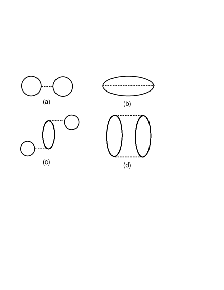
Figure 16: The diagrams of perturbation theory contributing to the pressure to order $g^{2}$ ((a) and (b)) and $g^{4}$ ((c) and (d)). The dotted line represents the fermionic interaction (proportional to $g^{2}/N$), not the full $\sigma$-propagator. The diagrams (a) and (c) are of order $N$, the diagrams (b) and (d) of order 1.

Consider then the first contribution:

$$P_{a}={g^{2}N\over 2}\left[\int{{\rm d}k\over 2\pi}{m\over E_{k}}(1-2n_{k})\right]^{2}$$ (166)

where $E_{k}=\sqrt{k^{2}+m^{2}}$ and $n_{k}=n(E_{k})$ is the fermion statistical factor (110). Note that $P_{a}$ is proportional to $\langle\bar{\psi}\psi\rangle^{2}$ (given by Eq. (18) with $M\to m$), from which one could guess that $P_{a}$ vanishes in the chiral limit $m=0$. However, as it stands, $P_{a}$ is ill defined and needs renormalisation. To do that, we rewrite $P_{a}$ as follows:

$$P_{a}={g^{2}N\over 2}\left\{\left[\int{{\rm d}k\over 2\pi}{m\over E_{k}}\right]^{2}-2\left[\int{{\rm d}k\over 2\pi}{m\over E_{k}}\right]\left[\int{{\rm d}k\over 2\pi}{m\over E_{k}}2n_{k}\right]+\left[\int{{\rm d}k\over 2\pi}{m\over E_{k}}2n_{k}\right]^{2}\right\},$$ (167)

The first term in the second line of Eq. (167) is a vacuum contribution and it can be discarded. The last term is finite. The potential difficulty comes from the second term which is divergent and temperature dependent. However such a divergence can be eliminated by a mass renormalization, i.e., by adding to the Lagrangian the counterterm $\delta m_{2}\,\bar{\psi}\psi$ with $\delta m_{2}$ chosen so as to cancel the correction of the zero temperature mass at order $g^{2}$, i.e.,

$$\delta m_{2}={g^{2}}N\int{{\rm d}k\over 2\pi}{m\over E_{k}}.$$ (168)

With the mass counterterm included, $P_{a}$ becomes

$$P_{a}\longrightarrow P^{\prime}_{a}=P_{a}+{g^{2}}N\int{{\rm d}k\over 2\pi}{m\over E_{k}}\int{{\rm d}k\over 2\pi}{m\over E_{k}}2n_{k},$$ (169)

and the unwanted contribution disappears in $P^{\prime}_{a}$, as expected.

Consider next the “exchange” term

$$P_{b}={g^{2}\over 2}\Pi(\tau\!=\!0,x\!=\!0;m,T),$$ (170)

One can notice that $\Pi(\tau\!=\!0,x\!=\!0;m,T)=\lim_{\tau\to 0}{\rm Tr}S(\tau,x\!=\!0;m,T)S(-\tau,x\!=\!0;m,T)$, where $S$ is the fermion propagator (see Eq. (C)), to write Eq. (170) as:

$$\Pi(\tau\!=\!0,x\!=\!0;m,T)\!=\!-\int{{\rm d}k\over 2\pi}\int{{\rm d}q\over 2\pi}\left\{\!-{1\over 2}\!-\!{m^{2}+k\,q\over 2E_{k}E_{q}}(1\!-\!2n_{k})(1\!-\!2n_{q})\right\}.$$ (171)

Note that before taking the limit $\tau\to 0$, the integrand in Eq. (171) contains exponential factors ${\rm e}^{\pm E_{k,q}\tau}$ which, together with statistical factors, insure the convergence of the integrals over $k$ and $q$. In the limit $\tau=0$, the first term in Eq. (171) is a divergent constant independent of the temperature and it can be ignored. The contribution proportional to $k\,q$ can be written as a product of two integrals which vanish by parity (at any finite $\tau$). What remains then in Eq. (170) is:

$$-{g^{2}\over 4}\left(\int{{\rm d}{k}\over 2\pi}{m\over E_{k}}(1-2n_{k})\right)\,\left(\int{{\rm d}{q}\over 2\pi}{m\over E_{q}}(1-2n_{q})\right)=-{P_{a}\over 2N}.$$ (172)

Thus the exchange term is just proportional to the direct contribution $P_{a}$ calculated above. It can be renormalized in the same way. We note now that all the contributions considered so far remain, after renormalization, proportional to $m$. It follows that all the contributions of order $g^{2}$ to the pressure cancel in the limit $m\to 0$: such contributions are proportional to $\langle\bar{\psi}\psi\rangle^{2}$, a quantity which vanishes when $m=0$.

Let us turn now to the first of the order $g^{4}$ contributions.

$$P_{c}=-{g^{4}N\over 2}\left[\int{{\rm d}k\over 2\pi}{m\over E_{k}}(1-2n_{k})\right]^{2}\Pi(0,0;m,T)=-g^{2}P_{a}\Pi(0,0;m,T)$$ (173)

where $\Pi(0,0;m,T)$ stands for $\Pi(\omega\!=\!0,q\!=\!0;m,T)$. One divergence contained in this quantity is eliminated by coupling constant renormalization. The needed counterterm is obtained form $P_{a}$ of Eq. (167) in which one replaces $g^{2}$ by $g^{2}+g^{4}\Pi_{0}(0,0;M_{0})$. One gets then:

$$P_{a}^{\prime\prime}={g^{2}N\over 2}\left[\int{{\rm d}k\over 2\pi}{m\over E_{k}}(1-2n_{k})\right]^{2}(1+g^{2}\Pi_{0}(0,0;M_{0}))$$ (174)

By combining $P_{c}$ and the order $g^{4}$ of $P_{a}^{\prime\prime}$, one gets

$$P_{c}^{\prime}=-{g^{4}N\over 2}\left[\int{{\rm d}k\over 2\pi}{m\over E_{k}}(1-2n_{k})\right]^{2}(\Pi(0,0;m,T)-\Pi_{0}(0,0;M_{0}))$$ (175)

where the quantity $\Pi(0,0;m,T)-\Pi_{0}(0,0;M_{0})$ is finite. The contribution $P_{c}^{\prime}$ is still divergent, but the divergences can be eliminated by the same procedure as that used above for $P_{a}$, namely by the mass renormalization counterterm. The result obtained at the end of this procedure is again proportional to $m$ and vanishes when $m\to 0$.

Note that the combination $\Pi(0,0;m,T)-\Pi_{0}(0,0;M_{0})$ in Eq. (175) enters also the calculation of the renormalized quark-quark scattering amplitude to order $g^{4}$ in perturbation theory:

$${\cal T}(0,0)=g^{2}-g^{4}\left[\Pi(0,0;T)-\Pi_{0}(0,0;M_{0})\right]=g^{2}-{g^{4}\over\pi}\ln{\pi T\over{\rm e}^{\gamma_{E}+1}M_{0}},$$ (176)

where the limit $m\to 0$ has already been taken (we used Eqs. (192), (194) and (208)). It can easily be verified that this expression is invariant under renormalization group transformations (to order $g^{4}$) when $g$ runs according to the lowest order $\beta$-function (97). Now, as usual in perturbation theory, one can choose the scale $M_{0}$ so as to minimize higher order corrections. In the present case, the order $g^{4}$ contribution to the scattering amplitude vanishes for $M_{0}=\pi T/{\rm e}^{\gamma_{E}+1}$. Note that for this choice of $M_{0}$,

$$g^{2}(M_{0}=\pi T/{\rm e}^{\gamma_{E}+1})={\pi\over\ln(T/T_{c})},$$ (177)

which, is the coupling constant $\tilde{g}^{2}$ introduced above, in Eq. (154). Note also that, for this choice, the quark-quark scattering amplitude in Eq. (176) coincides with that calculated within the non-perturbative scheme (see Eq. (149)).

Before we move on to the last order $g^{4}$ contribution (the only one to survive the limit $m\to 0$ which we implicitly assume from now on), let us return to the contribution $P_{b}$ given in Eq. (170), in order to make closer contact with the $1/N$ calculation. One can rewrite $P_{b}$ as

$$P_{b}={g^{2}\over 2}\int{{\rm d}q\over 2\pi}\int_{-i\infty+\epsilon}^{i\infty+\epsilon}\,{{\rm d}\omega\over 2\pi i}\,(1+2N(\omega))\,\Pi(\omega,q;T)=\Pi(\tau=0,x=0;T).$$ (178)

(By performing the $\omega$-integral and suitably rearranging the statistical factors, one can recover, form this expression, Eq. (171) above.) The quantity $\Pi(\omega,q;T)$ is ill defined, since it contains an infinite constant contribution, independent of the temperature. We can absorb this constant into $\Pi_{0}(0,0;M_{0})$ and discard the corresponding vacuum contribution. Next we write:

$$\Pi(\omega,q;T)-\Pi_{0}(0,0;M_{0})=\left[\Pi(\omega,q;T)-\Pi(0,0;T)\right]+\left[\Pi(0,0;T)-\Pi_{0}(0,0;M_{0})\right].$$ (179)

The last term within brackets is $(1/\pi)\ln\left(\pi T/M_{0}{\rm e}^{\gamma_{E}+1}\right)$ (see Eq. (176) above). The first term within brackets is $(1/2\pi)B_{T}(Q/T)$ which, at large Q, behaves as $(1/2\pi)\ln(Q^{2}T_{c}^{2}/(T^{2}M_{f}^{2}))$ (see App. A). This suggests the following temperature independent subtraction which transforms $P_{b}$ into

$$P_{b}^{\prime\prime}={g^{2}\over 4\pi}\int[{\rm d}^{2}Q]\left(B_{T}(Q/T)+\ln\left({\pi^{2}T^{2}\over M_{0}^{2}{\rm e}^{2(\gamma_{E}+1)}}\right)\right)-{g^{2}\over 4\pi}\int{{\rm d}^{2}q\over(2\pi)^{2}}\ln\left({Q_{E}^{2}\over M_{0}^{2}{\rm e}^{2}}\right).$$ (180)

At this stage, it is necessary to separate the integral into the part which contains the statistical factor, and the other which does not. The part with the statistical factor is calculated by deforming the contour in the usual way (see subsection IV.2) and yields:

$$P_{b}^{G}={g^{2}\over 2\pi^{3}}\int_{0}^{\infty}{\rm d}q\,\int_{0}^{\infty}{\rm d}\omega\,N(\omega)\,{\rm Im}B_{T}(\omega/T,q/T).$$ (181)

This contribution is independent of the vacuum subtraction. Changing to the dimensionless variables $s=\omega/T$, $r=q/T$, fixing the scale $M_{0}$ at the value $M_{0}=\pi T/{\rm e}^{\gamma_{E}+1}$ and identifying $g^{2}$ with the running coupling at that scale (i.e., replacing $g^{2}$ by $\tilde{g}^{2}$ in Eq. (181)), and finally multiplying by $(4\pi/M_{f}^{2})$ (see Eq. (126)) and dividing by $(T^{2}/M_{f}^{2})(\tilde{g}^{2}/2\pi)$ (see Eq. (162)), one recovers the expression (163) of $G_{2}$. The part without the statistical factor in $P_{b}^{\prime\prime}$ reads

$$P_{b}^{F}={g^{2}\over 4\pi}\int{{\rm d}^{2}q\over(2\pi)^{2}}\left(B_{T}(Q/T)+\ln\left({\pi^{2}T^{2}\over M_{0}^{2}{\rm e}^{2(\gamma_{E}+1)}}\right)\right)-{g^{2}\over 4\pi}\int{{\rm d}^{2}q\over(2\pi)^{2}}\ln\left({Q_{E}^{2}\over M_{0}^{2}{\rm e}^{2}}\right),$$ (182)

and it can be verified that it is finite. By choosing again $M_{0}=\pi T/{\rm e}^{\gamma_{E}+1}$, and substituting $\tilde{g}^{2}$ for $g^{2}$ in Eq. (182), one gets:

$$P_{b}^{F}={\tilde{g}^{2}\over 4\pi}\int{{\rm d}^{2}q\over(2\pi)^{2}}B_{T}(Q/T)-{\tilde{g}^{2}\over 4\pi}\int{{\rm d}^{2}q\over(2\pi)^{2}}\ln\left({Q_{E}^{2}T_{c}^{2}\over T^{2}M_{f}^{2}}\right).$$ (183)

The same manipulations as done before for $P_{b}^{G}$ allow us to recover the expression (156) of $F_{2}$.

At this point, we have all the necessary ingredients to understand the origin of the cancellation $F_{2}+G_{2}=0$ observed in the previous subsection. We have just seen that $P_{b}=P_{b}^{G}+P_{b}^{F}\propto F_{2}+G_{2}$; but from the calculation of $P_{b}$ done above with Eq. (170) we have $P_{b}=0$. Hence the cancellation. Consider finally

$$P_{d}={g^{4}\over 4}\int[{\rm d}^{2}Q]\left[\Pi(\omega,q;T)\right]^{2}.$$ (184)

We can proceed as we did for $P_{c}$ and first combine $P_{d}$ with the contribution coming from the coupling constant renormalization of $P_{b}$ which transforms $P_{b}$ into $P_{b}^{\prime}$:

$$P_{b}^{\prime}=P_{b}(1+g^{2}\Pi_{0}(0,0;M_{0}))=P_{b}-{g^{4}\over 2}\int[{\rm d}^{2}Q]\Pi(\omega,q;T)\Pi_{0}(0,0;M_{0}).$$ (185)

(Of course, according to the previous discussion, this is a vanishing correction, but it is convenient to carry it along as it makes the procedure more transparent.) By adding to $P_{d}$ the order $g^{4}$ contribution from $P_{b}^{\prime}$, we get:

$$P_{d}^{\prime}={g^{4}\over 4}\int[{\rm d}^{2}Q]\left[\Pi(\omega,q;T)-\Pi_{0}(0,0;M_{0})\right]^{2}$$ (186)

where we have also added an irrelevant constant $\sim(\Pi_{0}(0,0;M_{0}))^{2}$. The divergence in Eq. (186) is dealt with in analogy with what we just did for $P_{b}$. Thus we write

$$P_{d}^{\prime\prime}=\!{g^{4}\over 4}\!\int[{\rm d}^{2}Q]\left[{1\over 2\pi}B_{T}(Q/T)\!+\!{1\over\pi}\ln\left({\pi T\over M_{0}{\rm e}^{(\gamma_{E}+1)}}\right)\right]^{2}\!-\!{g^{4}\over 4}\!\int{{\rm d}^{2}q\over(2\pi)^{2}}\left[{1\over 2\pi}\!\ln\!\left({Q_{E}^{2}\over M_{0}^{2}{\rm e}^{2}}\right)\right]^{2}.$$ (187)

and it can be verified that $P_{d}^{\prime\prime}$ is finite.

At this stage, one may choose the scale to be $M_{0}=\pi T/{\rm e}^{\gamma_{E}+1}$. Then $P_{d}^{\prime\prime}$ simplifies into:

$$P_{d}^{\prime\prime}={\tilde{g}^{4}\over 4}\int[{\rm d}^{2}Q]\left[{1\over 2\pi}B_{T}(Q/T)\right]^{2}-{\tilde{g}^{4}\over 4}\int{{\rm d}^{2}q\over(2\pi)^{2}}\left[{1\over 2\pi}\ln\left({Q_{E}^{2}T_{c}^{2}\over M_{f}^{2}T^{2}}\right)\right]^{2}.$$ (188)

We can now perform the $\omega$-integral as we did earlier and separate the contributions containing one or no statistical factors. We obtain in this way the contribution of order $g^{4}$ to the functions $F$ and $G$. These are:

$$F_{4}=-{1\over\pi}\int_{0}^{\infty}{\rm d}s\int_{0}^{\infty}{\rm d}r\left(\left[B_{T}(is,r)\right]^{2}-\left[\ln\left(T_{c}^{2}/M_{f}^{2}(s^{2}+r^{2})\right)\right]^{2}\right),$$ (189)

$$G_{4}=-{4\over\pi}\int_{0}^{\infty}{\rm d}s\int_{0}^{\infty}{\rm d}rN(s){\rm Im}B_{T}(s,r){\rm Re}B_{T}(s,r),$$ (190)

which agrees with the expressions given above (Eqs. (157) and (164)).

To summarize, the perturbative calculation performed in this last subsection has allowed us to recover the high temperature limit obtained previously within the $1/N$ expansion. The calculation involves a running coupling at a scale $M_{0}$ which can be chosen, as usual in perturbation theory, so as to minimize the high order corrections. Here the choice $M_{0}=\pi T/{\rm e}^{\gamma_{E}+1}$ allows us to identify the running coupling with $\tilde{g}$ which naturally emerges in the high temperature expansion of the order $1/N$ calculation. We have seen that the second order terms vanish, because they are proportional to the quark condensate which vanish in the high temperature phase; this explains the cancellation of $F_{2}+G_{2}$ shown in the previous subsection. Finally, we have also been able to reproduce explicitly the analytical formulae giving the first few terms of the high temperature expansion of the pressure. This analysis confirms that, as could be expected from asymptotic freedom, the behavior of the system at high temperature can be understood in terms of perturbation theory.

VI Conclusions

The Gross-Neveu model in 1+1 dimension has proven to be a very useful playground to study various aspects of renormalization at finite temperature. We have obtained, at next-to-leading order in the $1/N$ expansion, a new expression for the effective potential, which is explicitly invariant under renormalization group transformations, both at zero and at finite temperature. We have verified, in a non-perturbative context, that the temperature dependent ultraviolet divergences cancel, as expected from general arguments: the same counterterms which make finite the effective potential at zero temperature also make it finite at non zero temperature. There is presently a lot of interest in exploring non perturbative techniques to study the thermodynamics of gauge fields, in particular of QCD vanHees:2002js ; Blaizot:2000fc ; Andersen:2000yj and the present investigations contribute to this general effort, in a much simpler context than that of gauge theories. In contrast to other methods, such as for instance those based on $\Phi$ derivable approximations vanHees:2002js ; Blaizot:2000fc , the $1/N$ expansion has the advantage of being at the same time non perturbative and of providing an expansion parameter: the latter is helpful to understand the systematics of the cancellation of ultraviolet divergences. Within this framework, there are obvious generalizations of the model studied in this paper, for example considering continuous symmetries and higher dimensions, which would be worth exploring.

Part of the motivation for studying the Gross-Neveu model specifically in 1+1 dimension is that it shares with three dimensional non abelian gauge theories like QCD the property of asymptotic freedom. This leads us to expect that at high temperature, the system behaves as a weakly interacting gas of the original constituents, somewhat analogous to the quark-gluon plasma of QCD. The detailed analysis of the high temperature limit is an important part of the present study. We have verified that, as expected from asymptotic freedom, the pressure can be expanded in terms of an effective coupling which decreases with increasing temperature. In fact, we have shown explicitly that, in this high temperature regime the prediction of the $1/N$ expansion is identical to that of ordinary perturbation theory. We find that the pressure goes slowly towards that of the ideal gas as the temperature increases. Compared to QCD where a similar phenomenon occurs, one finds that in the present calculation the pressure is higher than that of the free gas, while it is lower in QCD. In QCD, the dominant correction to the free gas behavior is of second order in the coupling strength, and the sign of the effect is easily understood from the corresponding expression of the entropy density Blaizot:2000fc . Here the contribution of the order $g^{2}$ cancels and the leading correction to the free gas behavior is of order $g^{4}$. Even if the basic mechanisms at work are different here and in QCD, it would be interesting to explore further the properties of the high temperature phase of the Gross-Neveu model along the lines developed in Ref. Blaizot:2000fc .

We find that the $1/N$ expansion provides a sensible approximation scheme at both low and high temperature: At low temperature, this is because it produces only small corrections to the mean field physics; at high temperature, it reproduces essentially perturbative calculations. But, for temperatures of the order of the mean field transition temperature the approximation breaks down: a Landau pole appears in the calculation and fluctuations become too large to be treated as corrections. (The Landau pole is harmless at low temperature and disappears at high temperature.) It would be interesting to explore further this breakdown of the $1/N$ expansion, in particular to study to which extent it is a consequence of the one-dimensional character of the system, by using different techniques, such as Exact Renormalization Group Equations, with which fermionic models have already been extensively studied at zero Ellwanger1994 and finite temperature Berges1999 (for a review see Berges2002 ). In this context, bosonic fluctuations can be included in a simple way, but the $1/N$ expansion has not been explored beyond the leading term.

Appendix A Renormalized $\sigma$ propagator

The bare fermion loop is defined in Eq. (22) and reads:

$$\Pi(Q;M,T)=2\int\{d^{2}{K}\}{M^{2}+{K}\cdot{K}^{\prime}\over(-{K}^{2}+M^{2})(-{K}^{\prime 2}+M^{2})}.$$ (191)

where the notation $\int\{d^{2}{K}\}$ is that of Eq. (5) and ${K}^{\prime}={K}+{Q}$. In this equation, and throughout this Appendix, $M$ is considered as a given parameter, not necessarily equal to the physical fermion mass $M_{f}$. Note that $\Pi(Q)$ is dimensionless.

One may perform the sum over the Matsubara frequencies (see Eq. (199) below) to verify that $\Pi$ can be written as a sum of a zero temperature contribution $\Pi_{0}$ and a finite temperature contribution $\tilde{\Pi}$ which goes to zero when $T\to 0$. This separation is well defined only when $M\neq 0$: indeed the zero temperature contribution, $\Pi_{0}(Q,M)$ is divergent when $M\to 0$. At finite temperature, the fermionic Matsubara frequencies provide an infrared cut-off which makes $\Pi(Q;M\to 0,T)$ well defined.

We consider first the zero temperature contribution $\Pi_{0}(Q;M)$. This may be obtained directly from Eq. (191) as an Euclidean integral, function of $Q_{E}^{2}=q_{0}^{2}+q^{2}$ only. Once regularized with a cut-off $\Lambda$, it yields:

$$\Pi_{0}(Q_{E};M)={1\over 2\pi}\left[\ln\left({M^{2}\over\Lambda^{2}}\right)+B_{0}\left({Q_{E}^{2}\over M^{2}}\right)\right],$$ (192)

where

$$B_{0}(z)\equiv\sqrt{{4+z\over z}}\ln\left[{\sqrt{4+z}+\sqrt{z}\over\sqrt{4+z}-\sqrt{z}}\right]$$ (193)

is an analytic function of $z$ with a cut on the negative real axis. Some properties of $B_{0}(z)$ for $z=x$ real and positive are useful. For small $x$

$$B_{0}(x)=2+{x\over 6}-{x^{2}\over 60}+{\cal O}(x^{3}),$$ (194)

while for large $x$

$$B_{0}(x)=\ln x+{2\over x}(1+\ln x)+{\cal O}\left({a+b\ln x\over x^{2}}\right).$$ (195)

The expression $1+g^{2}_{B}\Pi_{0}(Q;M)$ may be interpreted as the bare inverse propagator for the $\sigma$ field in leading order of the $1/N$ expansion (see Eq. (21)). The renormalized inverse propagator is obtained by multiplying it by $Z$ (coming from the renormalization of $\tilde{\sigma}$ in Eq. (21)), and replacing $g^{2}_{B}$ by $g^{2}/Z$, with $Z=Z^{(0)}=(g^{2}/\pi)\ln(\Lambda/M_{f})$ (see Eq. (51) with $\bar{Z}^{(0)}=0$). One then obtains:

$$D_{0}^{-1}(Q_{E};M) = Z\left(1+{g^{2}\over Z}\Pi_{0}(Q_{E};M)\right)={g^{2}\over 2\pi}\left[\ln\left({M^{2}\over M_{f}^{2}}\right)+B_{0}\left({Q_{E}^{2}\over M^{2}}\right)\right]$$ (196)

$$= {g^{2}\over\pi}\ln\left({M\over M_{f}}\right)+{g^{2}\over 2\pi}\sqrt{1+{4M^{2}\over Q_{E}^{2}}}\ln\left[{Q_{E}^{2}\over 4M^{2}}\left(1+\sqrt{1+{4M^{2}\over Q_{E}^{2}}}\right)^{2}\right].$$

This is an increasing function of $Q_{E}^{2}$, whose minimum, at $Q_{E}^{2}=0$, coincides, up to a factor $g^{2}$ (see Eq. (27)), with the second derivative with respect to $M$ of the leading order contribution to the renormalized effective potential (Eq. (55)):

$$D^{-1}_{0}(Q_{E}=0;M)={g^{2}\over\pi}\left(1+\ln{M\over M_{f}}\right)=g^{2}{{\rm d}^{2}V^{(0)}\over{\rm d}M^{2}}.$$ (197)

Note that $D^{-1}_{0}(Q_{E}=0;M)$ vanishes at the value $M_{*}=M_{f}/e$. For $M>M_{*}$, $D^{-1}_{0}(Q_{E};M)$ is always positive; for $M<M_{*}$, $D^{-1}_{0}(Q_{E};M)$ vanishes at some positive value of $Q_{E}^{2}$ and is negative for smaller values of $Q_{E}^{2}$. That is, when $M\leq M_{*}$ the $\sigma$ propagator has an unphysical pole, whose role in the next-to-leading order calculation of the effective potential is discussed in the main text.

For large values of $Q_{E}^{2}$, we obtain from Eq. (195):

$$D^{-1}_{0}(Q_{E};M)\simeq{g^{2}\over 2\pi}\left[\ln\left({Q_{E}^{2}\over M^{2}_{f}}\right)+{2M^{2}\over Q_{E}^{2}}\left(1+\ln{Q_{E}^{2}\over M^{2}}\right)\right]+{\cal O}\left({M^{3}\over Q_{E}^{3}}\ln{Q_{E}^{2}\over M^{2}}\right).$$ (198)

We now turn to the finite temperature contribution, $\tilde{\Pi}(\omega,q;M,T)$. This is obtained from Eq. (191) by performing the sum over Matsubara frequencies. The resulting expression for the total $\Pi$ is:

$$\Pi_{0}(\omega,q;M)+\tilde{\Pi}(\omega,q;M,T)=-\int_{-\infty}^{\infty}{{\rm d}k\over 2\pi}$$ (199)

$$\left[{E_{+}\,E_{-}+M^{2}-k^{2}+q^{2}/4\over 2E_{+}\,E_{-}}\left({n_{+}-n_{-}\over\omega-E_{+}+E_{-}}-{n_{+}-n_{-}\over\omega+E_{+}-E_{-}}\right)\right.$$

$$+\left.{E_{+}\,E_{-}-M^{2}+k^{2}-q^{2}/4\over 2E_{+}\,E_{-}}\left({n_{+}+n_{-}-1\over\omega-E_{+}-E_{-}}-{n_{+}+n_{-}-1\over\omega+E_{+}+E_{-}}\right)\right],$$

where

$$E_{\pm}=\sqrt{(k\pm q/2)^{2}+M^{2}},\qquad\qquad n_{\pm}\equiv n(E_{\pm})={1\over{\rm e}^{\beta E_{\pm}}+1}.$$ (200)

The finite temperature contribution proper, i.e., $\tilde{\Pi}(\omega,q;M,T)$, is obtained by keeping only terms proportional to statistical factors (i.e., by dropping the 1’s in the third line of Eq. (199)). One can then verify that

$$\tilde{\Pi}(\omega,q)=\tilde{\Pi}(-\omega,q)=\tilde{\Pi}(\omega,-q).$$ (201)

Thus we need to calculate $\tilde{\Pi}$ only in the region $\omega>0$, $q>0$. Note also that changing $k$ into $-k$ in the integrand of Eq. (199) is equivalent to changing $q$ into $-q$ which leaves the integrand invariant; we can therefore limit the $k$-integration to the range $[0,\infty[$.

The imaginary part is defined as usual as the imaginary part of $\tilde{\Pi}(\omega+i\epsilon,q)$ with $\omega$ real. In the region of interest, this is non vanishing for $k$ values such that (a): $E_{+}-E_{-}=\omega$, or (b): $E_{+}+E_{-}=\omega$. The case (a) is typical of finite temperature and corresponds to scattering processes in the heat bath. The case (b) corresponds to processes which are analogous to those occurring at zero temperature (decay of the sigma into quark-antiquark pairs; see Sect. V.2). For each value of $\omega$ and $q$, the “phase-space” is limited to a single value of the momentum and the energy of the quark. This is given by ($\omega_{q}=\sqrt{q^{2}+4M^{2}}$):

$$(a)\qquad 0<\omega<q\qquad\qquad{\rm(scattering\,processes)}\qquad\qquad\qquad\qquad\qquad\qquad$$

$$k^{a}={\omega\over 2}\sqrt{{\omega_{q}^{2}-\omega^{2}\over q^{2}-\omega^{2}}}\qquad E^{a}_{\pm}={1\over 2}\left(\pm\omega+q\sqrt{{\omega_{q}^{2}-\omega^{2}\over q^{2}-\omega^{2}}}\right)\qquad$$ (202)

$$(b)\qquad\omega>\omega_{q}\qquad\qquad{\rm(pair\,creation)}\qquad\qquad\qquad\qquad\qquad\qquad$$

$$k^{b}={\omega\over 2}\sqrt{{\omega^{2}-\omega_{q}^{2}\over\omega^{2}-q^{2}}}=k^{a}\qquad E^{b}_{\pm}={1\over 2}\left(\omega\pm q\sqrt{{\omega^{2}-\omega_{q}^{2}\over\omega^{2}-q^{2}}}\right)\qquad$$ (203)

The corresponding imaginary parts are given by:

$$(a)\qquad 0<\omega<q\qquad\qquad{\rm Im}\tilde{\Pi}={1\over 2}\sqrt{{\omega_{q}^{2}-\omega^{2}\over q^{2}-\omega^{2}}}\,\left(n(E_{+}^{a})-n(E_{-}^{a})\right)$$ (204)

$$(b)\qquad\omega>\omega_{q}\qquad{\rm Im}\tilde{\Pi}={1\over 2}\sqrt{{\omega^{2}-\omega_{q}^{2}\over\omega^{2}-q^{2}}}\,\left(n(E_{+}^{b})+n(E_{-}^{b})\right)$$ (205)

For $\omega>0$ outside the regions $[0,q]$ and $[\omega_{q},\infty[$, ${\rm Im}\tilde{\Pi}=0$. The real parts are determined as principal value integrals.

Note that the contribution of the scattering processes to the imaginary part is negative, while that of the pair creation processes is positive. In fact, in order to get a physically meaningfull result, the latter should be added to the (negative) zero temperature contribution (see Eq. (142)): the finite temperature contribution can then be interpreted as a “suppression” of pair creation due to Pauli blocking.

Consider now $\Pi$ in Eq. (199), and take the limit $M\to 0$. We get:

$$\Pi(\omega,q;T)=-\!\!\int_{0}^{\Lambda/2}{{\rm d}k\over\pi}\,{4k\over\omega^{2}-4k^{2}}\left[{1\over{\rm e}^{\beta(k+q/2)}+1}-{1\over{\rm e}^{\beta(q/2-k)}+1}\right],$$ (206)

where we have used the property

$${1\over{\rm e}^{\beta(k-q/2)}+1}-1=-{1\over{\rm e}^{\beta(q/2-k)}+1}$$ (207)

to rearrange terms. The ultraviolet cut-off $\Lambda/2$ (rather than $\Lambda$) is chosen so that $Z+g^{2}\Pi$ coincides with the previously defined renormalized inverse propagator in the limit $M\to 0$. Indeed, we have

$$\Pi(0,0;T)=\!\!\int_{0}^{\Lambda/2}{{\rm d}k\over\pi}\,{1\over k}\left[{1\over{\rm e}^{\beta k}+1}-{1\over{\rm e}^{-\beta k}+1}\right]={1\over\pi}\ln\left({\pi T\over{\rm e}^{\gamma_{E}}\Lambda}\right),$$ (208)

where the second equality holds up to terms which vanish when $\Lambda\to\infty$. Combining this result with the expression (51) of the renormalization constant $Z$ (with $\bar{Z}^{(0)}=0$), and using Eq. (134), we get

$$Z+g^{2}\Pi(0,0;T)={g^{2}\over\pi}\ln\left({T\over T_{c}}\right).$$ (209)

As expected, up to the factor $g^{2}$, this is the second derivative of the effective potential at $M=0$ (see Eqs. (147) and (149)).

The inverse propagator at $M=0$ is then:

$$D^{-1}(\omega,q;T)=Z+g^{2}\Pi(\omega,q;T)=Z+g^{2}\Pi(0,0;T)+g^{2}[\Pi(\omega,q;T)-\Pi(0,0;T)]$$ (210)

where the combination $\Pi(\omega,q;T)-\Pi(0,0;T)\equiv(1/2\pi)B_{T}(Q/T)$ is finite. Thus, in analogy with Eq. (141), we write

$$D^{-1}(\omega,q;T)={g^{2}\over 2\pi}\left[\ln\left({T^{2}\over T_{c}^{2}}\right)+B_{T}\left({\omega\over T},{q\over T}\right)\right].$$ (211)

Thus defined, the dimensionless function $B_{T}(\omega/T,q/T)$ behaves as $\ln(T_{c}^{2}/M_{f}^{2}(-\omega^{2}+q^{2})/T^{2})+\mathcal{O}(T^{4}/(q^{2}-\omega^{2})^{2})$ when $q\gg T$ or $\omega\gg T$. At small $\omega,q$, $B_{T}$ is regular ($B_{T}(\omega/T,q/T)\to 0$ as $\omega,q\to 0$).

Figure 17: The function ${\rm Re}B_{T}(s,r)$

The imaginary part of $D^{-1}(\omega,q;T)$ is finite and given simply by ($\omega$ real and positive):

$${\rm Im}\Pi(\omega,q;T)={1\over 2}\,\left({1\over{\rm e}^{\beta(q+\omega)/2}+1}-{1\over{\rm e}^{\beta(q-\omega)/2}+1}\right).$$ (212)

At small $\omega$, and as long as $q\mathrel{\hbox to0.0pt{\raise 2.20013pt\hbox{$<$}\hss}{\lower 2.20013pt\hbox{$\sim$}}}T$, ${\rm Im}\Pi(\omega,q;T)$ is a linear function of $\omega$, with a slope $-q/4T$. When $q>T$ however, the slope vanishes exponentially, as $(q/T)\exp(-q/T)$. For large values of $q/T$, the imaginary part becomes a step function of height -1/2 located at $\omega=q$.

The real part is obtained numerically from the principal value of the integral (206), by combining with the renormalization constant to eliminate the cut-off. It can be also expressed in terms of the real part of the function $B_{T}$:

$${\rm Re}B_{T}(s,r)={\rm PP}\int_{0}^{\infty}{\rm d}x\left[{x\over x^{2}-r^{2}/4}(n_{+}-n_{-})-{1\over x}(f_{+}-f_{-})\right],$$ (213)

where we have set $x\equiv k/T$, $s\equiv\omega/T$, $r\equiv q/T$, and

$$f_{\pm}={1\over{\rm e}^{\pm x}+1}\qquad\qquad n_{\pm}={1\over{\rm e}^{{s\over 2}\pm x}+1}.$$ (214)

A plot of ${\rm Re}B_{T}(s,r)$ is given in Fig. 17.

Let us finally examine the asymptotic behavior of $\Pi(\omega,q)$ when $q$ (or $\omega$) is large. This is dominated by the zero temperature contribution and the leading term is given by Eq. (198). However, at next-to-leading order, there is a relevant contribution coming from $\tilde{\Pi}$. To estimate it, we go back to Eq. (199), change $\omega\to iq_{0}$ and to go to polar coordinates: $q_{0}=r\cos\theta$, $q=r\sin\theta$. Next, one performs changes of variables such that all the statistical factors in Eq. (199) have the same energy argument. Then it is not hard to get:

$$\tilde{\Pi}(iq_{0},q)\sim\int_{-\infty}^{\infty}{{\rm d}k\over 2\pi}{n_{k}\over E_{k}}\left[8k^{2}-8\sin^{2}\theta(E_{k}^{2}+k^{2})\right]{1\over r^{2}}.$$ (215)

In particular,

$$\int_{0}^{2\pi}{{\rm d}\theta\over 2\pi}\tilde{\Pi}(iq_{0},q)\sim-{4M^{2}\over r^{2}}\int_{-\infty}^{\infty}{{\rm d}k\over 2\pi}{n_{k}\over E_{k}}.$$ (216)

Appendix B The functions $F_{0}(x)$, $F(x,T)$ and $G(x,T)$

The function $F_{0}(x)$ introduced in Eq. (73) of the main text is defined by:

$$F_{0}(x)\equiv{1\over 2}\int_{e^{2}}^{\infty}du\left\{\ln\left[{\ln x+B_{0}(u/x)\over B_{0}(u)}\right]-2{x-1\over u}-2{x-1-x\ln x\over u\ln u}\right\}$$

$$+{1\over 2}\int_{0}^{e^{2}}du\ln\left[{\ln x+B_{0}(u/x)\over B_{0}(u)}\right]\;.$$ (217)

The last two terms in the first line of this equation correspond to the $\Lambda$-dependent terms in Eq. (65), which we have rewritten as:

$${1\over 4\pi}\ln{\Lambda^{2}\over M_{f}^{2}} = \int_{eM_{f}}^{\Lambda}{1\over(2\pi)^{2}}{d^{2}Q\over Q^{2}}+{1\over 2\pi},$$

$${1\over 4\pi}\ln\ln{\Lambda\over M_{f}} = \int_{eM_{f}}^{\Lambda}{1\over(2\pi)^{2}}{d^{2}Q\over Q^{2}\ln(Q^{2}/M_{f}^{2})}.$$ (218)

Thus, by combining the integrand as we did in Eq. (B), we have obtained convergent integrals and the limit $\Lambda\to\infty$ could be taken. Note that, as stated in subsection III.2, the function $F_{0}(x)$ is defined only for $x>x_{M_{*}}=1/{\rm e}^{2}$.

To find the first derivative $F_{0}^{\prime}$, it is convenient to separate the contribution of the last two terms of the first line of Eq. (B), which we call $F^{\prime}_{\rm CT}$. Since $F^{\prime}_{\rm CT}$ is divergent, we re-introduce a cut-off $\Lambda$, and get:

$$F^{\prime}_{\rm CT}=\int_{e^{2}}^{\Lambda^{2}}{{\rm d}u\over u}\left(-1+{\ln x\over\ln u}\right).$$ (219)

In order to calculate the remaining contribution to $F_{0}^{\prime}(x)$, we use the change of variables

$$v={u\over 4x}\left(1+\sqrt{{4x\over u}+1}\right)^{2}$$ (220)

to get

$$F^{\prime}_{0}(x)-F^{\prime}_{\rm CT}(x)=\int_{1}^{\alpha}{{\rm d}v\over v}{\ln v\over\ln x+{v+1\over v-1}\ln v},$$ (221)

where $\alpha\equiv v(u=\Lambda^{2})\sim\Lambda^{2}/x$ for large $\Lambda$. In order to recombine both contributions (219) and (221), and let $\Lambda\to\infty$, one observes that

$$\int_{e^{2}}^{\Lambda^{2}}{{\rm d}u\over u}\left(-1+{\ln x\over\ln u}\right)=\int_{e^{2}}^{\Lambda^{2}/x}{{\rm d}u\over u}\left(-1+{\ln x\over\ln u}\right)-\ln x+{\cal O}(\ln x/\ln\Lambda^{2}).$$ (222)

Thus, adding (221) and (222) and now letting $\Lambda\to\infty$, one gets after simple algebra:

$$F^{\prime}_{0}(x) = \ln x\int_{e^{2}}^{\infty}{{\rm d}u\over u}\left({1\over\ln u}-{(u-1)^{2}\over(u^{2}-1)\ln x+(u+1)^{2}\ln u}\right)$$ (223)

$$+ \int_{1}^{e^{2}}{{\rm d}u\over u}{\ln u\over\ln x+{u+1\over u-1}\ln u}-\ln x-2\ln(e^{2}+1)+4.$$

The second derivative $F^{\prime\prime}_{0}$ follows easily from the previous expression. One has:

$$xF^{\prime\prime}_{0}(x)+1=\int_{e^{2}}^{\infty}{{\rm d}u\over u}\left({1\over\ln u}-{\ln u\over(\ln x+{u+1\over u-1}\ln u)^{2}}\right)-\int_{1}^{e^{2}}{{\rm d}u\over u}{\ln u\over(\ln x+{u+1\over u-1}\ln u)^{2}}$$ (224)

Finally, the third derivative $F_{0}^{\prime\prime\prime}$, needed for instance to calculate the $\beta$-function at next-to-leading order, is obtained by taking the derivative of the expression above:

$$x^{2}F^{\prime\prime\prime}_{0}(x)+xF^{\prime\prime}_{0}(x)=2\int_{1}^{\infty}{{\rm d}u\over u}{\ln u\over(\ln x+{u+1\over u-1}\ln u)^{3}}$$ (225)

Note that $F^{\prime}_{0}$, $xF^{\prime\prime}_{0}$ and $x^{2}F^{\prime\prime\prime}_{0}+xF^{\prime\prime}_{0}$ are actually functions of the variable $\ln x$. In the main text we use the limit of these expressions as $\ln x\to\infty$. This limit is easily obtained from the equations above. On finds:

$$F^{\prime}_{0}(x)\sim(\ln x)(\ln\ln x)\hskip 28.45274ptxF^{\prime\prime}_{0}(x)\sim\ln\ln x\hskip 19.91684pt{\rm and}\hskip 19.91684ptxF^{\prime\prime}_{0}+x^{2}F^{\prime\prime\prime}_{0}(x)\sim 1/\ln x.$$ (226)

We turn now to the function $F(x,T)$ which is obtained when we regroup what remains of $V^{(1)}_{b,1}$ after elimination of the temperature dependent divergence in Eq. (123) with the function $F_{0}$ introduced above, Eq. (B). We define:

$${M^{2}_{f}\over 4\pi}F(x_{M},T)\equiv{M^{2}_{f}\over 4\pi}F_{0}(x_{M})+{1\over 2}\int^{eM_{f}}_{0}{rdr\over 2\pi}\int^{2\pi}_{0}{d\theta\over 2\pi}\ln\left[{D^{-1}(r,\theta;M)\over D^{-1}_{0}(r^{2};M_{f})}\right]$$

$$+{1\over 2}\int^{\infty}_{eM_{f}}{rdr\over 2\pi}\left\{\int^{2\pi}_{0}{d\theta\over 2\pi}\ln\left[{D^{-1}(r,\theta;M)\over D^{-1}_{0}(r^{2};M_{f})}\right]+{8M^{2}\over r^{2}\ln(r^{2}/M^{2}_{f})}\left(\int_{0}^{\infty}du{n_{u}\over\sqrt{u^{2}+x_{M}}}\right)\right\}.$$

In this equation we have set $\omega=iq_{0}$ and changed to polar coordinates: $q_{0}=r\cos\theta$, $q=r\sin\theta$. Also, we use abusively the notation $D^{-1}(r,\theta)$ for $D^{-1}(\omega=ir\cos\theta,q=r\sin\theta)$, and similarly for $D_{0}^{-1}$. To get the last term in the expression above we used the second equation in (B) and the fact that $\ln\ln\Lambda/M_{f}=\ln\ln\Lambda/M+{\cal O}(1/\ln(\Lambda/M_{f}))$. Note finally that, since $F$ contributes to a term of order $1/N$, we have set $x_{M}=M^{2}/M^{2}_{f}$, ignoring the factor of order $1/N$ in Eq. (86). One has:

$$F(x,T) = \int^{\infty}_{e}2\,v\,dv\;\;\left\{\int^{\pi/2}_{0}{d\theta\over\pi}\ln(A(v,\theta;x,T))\right.$$ (228)

$$- \left.{x-1\over v^{2}}-{1\over v^{2}\ln v^{2}}\left(x-1-x\ln x\;-4x\;\int_{0}^{\infty}du{n_{u}\over\sqrt{u^{2}+x}}\right)\right\}$$

$$+ \int^{e}_{0}2\,v\,dv\int^{\pi/2}_{0}{d\theta\over\pi}\ln(A(v,\theta;x,T))$$

where the function $A(v,\theta;x,T)$ is

$$A={\ln x+B_{0}(v^{2}/x)+2\pi\tilde{\Pi}(v,\theta;x,T)\over B_{0}(v^{2})}.$$ (229)

In (228) we have used the symmetry properties (201) to limit the integration over $\theta$ to the interval $[0,\pi/2]$. Note finally that $F(x,T=0)=F_{0}(x)$, with $F_{0}$ given by Eq. (B). The function $F(x,T)$, evaluated numerically, is shown in Fig. 18, for various values of $T$. Note that, when $T<T_{c}$, $F(x_{M},T)$ is defined only for $x_{M}>x_{M_{*}}(T)$ (see subsection IV.2).

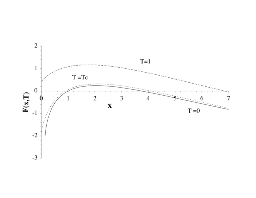
Figure 18: The function $F(x,T)$ for various temperatures. Full line: $T=0$, i.e., $F_{0}(x)$; dotted line: $T=0.565M_{f}=T_{c}$; dashed line: $T=M_{f}$

To study the high temperature limit of the the function $F(x_{M},T)$ (needed in subsection V.4) it is useful to write $F(x_{M}=0,T)$ in a different form. Adding and subtracting the expression

$$\int_{0}^{\infty}2vdv\int_{0}^{\pi/2}{d\theta\over\pi}\ln\left({B_{0}(v^{2})\over\ln(\sqrt{1+v^{4}})}\right)$$ (230)

we can rewrite $F(0,T)$ as

$$F(0,T)={T^{2}\over M_{f}^{2}}{2\over\pi}\int_{0}^{\infty}ds\int_{0}^{\infty}dr\ln\left({\ln(T^{2}/T_{c}^{2})+B_{T}(is,r)\over\ln(\sqrt{1+(s^{2}+r^{2})T^{4}/M_{f}^{4}})}\right)$$

$$+ \int_{e}^{\infty}2vdv\left\{\int_{0}^{\pi/2}{d\theta\over\pi}\ln\left({\sqrt{1+v^{4}}\over B_{0}(v^{2})}\right)+{1\over v^{2}}+{1\over v^{2}\ln v^{2}}\right\}+\int_{0}^{e}2vdv\int_{0}^{\pi/2}{d\theta\over\pi}\ln\left({\sqrt{1+v^{4}}\over B_{0}(v^{2})}\right)$$

In the first line we introduced the function $B_{T}$ (defined in App. A) and made the change of variables $s=(M_{f}/T)v\cos\theta$, $r=(M_{f}/T)v\sin\theta$. It is a finite expression (see the comment after Eq. (211)). The second line is also finite (see Eq. (195)) and it is independent of the temperature.

Finally the function $G$ is

$$G(x,T)=-{4\over\pi}\int_{0}^{\infty}dr\int_{0}^{\infty}dsN(s)\,\delta(s,r;x,T).$$ (232)

where $\delta$ is given by Eq. (129). We have set here $s=\omega/M_{f}$, $r=q/M_{f}$ and $N(s)=1/(e^{bs}-1)$. The function $G(x,T)$, evaluated numerically, is presented in Fig. 19 for various temperatures.

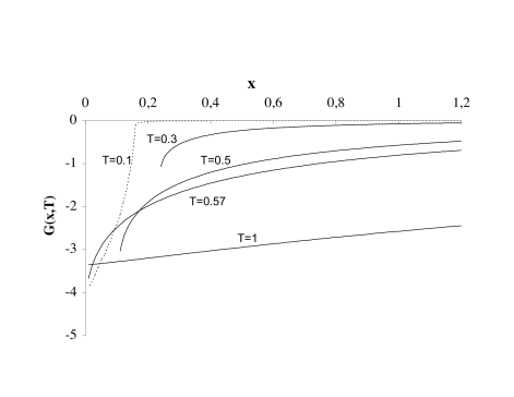
Figure 19: The function $G(x,T)$ versus $x$ for various temperatures $T$ (in units of the fermion mass $M_{f}$). The dotted line corresponds to $T/M_{f}=0.1$ and indicates the typical behavior of the function for small values of $x$ when $T<T_{c}$. For the other temperatures the function is plotted only for $x>x_{M_{*}}(T)$.

One can understand the behavior of $G$ at small $x_{M}$ from the behavior of the phase shift. At moderate temperatures it is enough to consider the zero temperature phase-shift in evaluating the integral in Eq. (232). For $M=M_{f}$, using the expression of the zero temperature propagator $D_{0}^{-1}(\omega,q;M_{f})$ given in App. A, we find ($\omega_{q}=\sqrt{q^{2}+4M^{2}_{f}}$):

$$\tan(\delta)={\pi\over 2}{\Theta(\omega-\omega_{q})\over{\rm Arctanh}\sqrt{(\omega^{2}-\omega_{q}^{2})/(\omega^{2}-q^{2})}}.$$ (233)

Consider this expression for fixed $q$, as a function of $\omega$. For $\omega\mathrel{\hbox to0.0pt{\raise 2.20013pt\hbox{$>$}\hss}{\lower 2.20013pt\hbox{$\sim$}}}\omega_{q}$ this behaves as $\delta(\omega,q)\sim{\pi}/{2}-({2}/{\pi})\sqrt{(\omega^{2}-\omega_{q}^{2})/(\omega^{2}-q^{2})}$ while at large $\omega$, $\delta(\omega,q)\sim\pi/\ln(\omega^{2}-q^{2})$. For $M\neq M_{f}$, $D_{0}^{-1}(\omega,q;M)=D_{0}^{-1}(\omega,q;M_{f})+(g^{2}/\pi)\ln(M/M_{f})$. A plot of ${\rm Re}D_{0}^{-1}(\omega,q;M)$ is given in Fig. 12. For $M<M_{f}$, the real part of $D_{0}^{-1}(\omega,q;M)$ vanishes at points $\omega_{a}$ and $\omega_{b}$ and is minimum at the point $\omega_{q}$ where it vanishes for $M=M_{f}$ ($\omega_{a}\leq\omega_{q}\leq\omega_{b}$). For $\omega<\omega_{a}$, $\delta$ is small and positive; it jumps to a value close to $\pi$ when $\omega$ crosses the value $\omega_{a}$, and remains approximately constant until $\omega\simeq\omega_{q}$, at which point it decreases rapidly to reach the value $-\pi/2$ at $\omega_{b}$; it then goes slowly to zero as $\omega\to\infty$. When $M\to M_{*}(T)$ from above, $\omega_{a}\to 0$, and the region $\omega<\omega_{q}$, where $\delta\simeq\pi$, gives a large contribution to $G$, amplified by the large value of the statistical factor at small $\omega$, where $N(\omega)\simeq T/\omega$. This is the origin of the large negative contribution at small $x_{M}$ that is visible in Fig. 19, particularly in the curve labelled $T=0.1M_{f}$.

Appendix C The fermion self-energy

Here we calculate the fermion self-energy defined in Eq. (35). We have:

$$\Sigma(K)=-{g^{2}\over N}\int[{\rm d}^{2}Q]\,D(Q;M)\,{(\hbox to0.0pt{\hbox to9.20833pt{\hfil/\hfil}\hss}K-\hbox to0.0pt{\hbox to7.90555pt{\hfil/\hfil}\hss}Q)+M\over-(K-Q)^{2}+M^{2}}\equiv a\hbox to0.0pt{\hbox to9.20833pt{\hfil/\hfil}\hss}K+b,$$ (234)

where $M$ is the renormalized mass, and $g$ the renormalized coupling. The functions $a(K)$ and $b(K)$ can be obtained easily by projection:

$$a(K)={1\over 2K^{2}}{\rm Tr}\hbox to0.0pt{\hbox to9.20833pt{\hfil/\hfil}\hss}K\Sigma(K)=-{g^{2}\over NK^{2}}\int[{\rm d}^{2}Q]\,D(Q;M)\,{K^{2}-K\cdot Q\over-(K-Q)^{2}+M^{2}},$$ (235)

$$b(K)={1\over 2}{\rm Tr}\Sigma(K)=-{g^{2}\over N}\int[{\rm d}^{2}Q]\,D(Q;M)\,{M\over-(K-Q)^{2}+M^{2}}.$$ (236)

One can separate the self-energy $\Sigma$ into a zero temperature contribution and a finite temperature one, as we did for the fermion loop in App. A. Accordingly we write:

$$\Sigma(K)=\Sigma_{0}(K)+\tilde{\Sigma}(K)$$ (237)

and similarly for the functions $a(K)$ and $b(k)$. It will be verified shortly that $a(K)$ is finite, while $b(K)$ is divergent. The divergence is a mass correction which is eliminated by the mass counterterm $Z^{\prime(1)}$. Introducing a cut-off $\Lambda$, one can write:

$$b(K)=-{M\over 2N}\ln\ln\left({\Lambda^{2}\over M_{f}^{2}}\right)+{M\over N}b^{\prime}(K),$$ (238)

where, as we shall verify, $b^{\prime}(K)$ is finite. The full fermion two-point function takes then the form:

$$S^{-1}(K) = -\hbox to0.0pt{\hbox to9.20833pt{\hfil/\hfil}\hss}K(1-a)+M\left(1+{Z^{\prime(1)}\over 2N}\right)+b(K)$$ (239)

$$= -\hbox to0.0pt{\hbox to9.20833pt{\hfil/\hfil}\hss}K\left(1-a(K)\right)+M\left(1+{\bar{Z}^{\prime(1)}\over 2N}+b^{\prime}(K)\right)$$

where we have used $M_{B}=\sqrt{Z^{\prime}}M$, $\sqrt{Z^{\prime}}=1+Z^{\prime(1)}/2N$ and $Z^{\prime(1)}=\ln\ln(\Lambda/M_{f})+\bar{Z}^{\prime(1)}$.

We now proceed to the explicit calculation of the zero temperature contribution to $\Sigma$. The corresponding functions $a_{0}$ and $b_{0}$ are functions of $K^{2}$ only. By going over to Euclidean momenta, and performing the angular integrals, one obtains:

$$b_{0}^{\prime}(K_{E}^{2})=-{g^{2}\over N}\int_{0}^{\Lambda^{2}}{{\rm d}Q_{E}^{2}\over 4\pi}{D_{0}(Q_{E}^{2};M)\over\sqrt{(K_{E}^{2}+M^{2}+Q_{E}^{2})^{2}-4K_{E}^{2}Q_{E}^{2}}}+{1\over 2N}\ln\ln{\Lambda\over M_{f}},$$ (240)

and

$$a_{0}(K_{E}^{2})=-{g^{2}\over N}\int{{\rm d}Q_{E}^{2}\over 8\pi K_{E}^{2}}\,D_{0}(Q_{E}^{2};M)\left(1+{K_{E}^{2}-Q_{E}^{2}-M^{2}\over\sqrt{(K_{E}^{2}+M^{2}+Q_{E}^{2})^{2}-4K_{E}^{2}Q_{E}^{2}}}\right).$$ (241)

One can verify on these explicit expressions that both $a_{0}(K^{2})$ and $b_{0}^{\prime}(K^{2})$ are finite.

In fact we shall need these functions only for $M=M_{f}$ and $K_{E}^{2}=-M_{f}^{2}$, and we shall set $a_{0}\equiv a_{0}(K_{E}^{2}=-M_{f}^{2})$, $b_{0}^{\prime}\equiv b_{0}^{\prime}(K_{E}^{2}=-M_{f}^{2})$. We have:

$$a_{0}={g^{2}M_{f}^{2}\over N}\int_{0}^{\infty}{{\rm d}Q^{2}\over 2\pi}{D_{0}(Q_{E}^{2};M_{f})\over(Q^{2}+2M_{f}^{2})\sqrt{Q^{4}+4M_{f}^{2}Q^{2}}+Q^{4}+4Q^{2}M_{f}^{2}}$$ (242)

$$b_{0}^{\prime}={1\over 2N}\int_{e^{2}M_{f}^{2}}^{\Lambda^{2}}{{\rm d}Q^{2}\over Q^{2}}{1\over\ln(Q^{2}/M_{f}^{2})}-{g^{2}\over N}\int_{0}^{\Lambda^{2}}{{\rm d}Q^{2}\over 4\pi}{D_{0}(Q_{E}^{2};M_{f})\over\sqrt{Q^{4}+4M_{f}^{2}Q^{2}}}.$$ (243)

By using the explicit expression (196) of the propagator together with the change of variables:

$$u=\sqrt{{Q^{2}\over 4M_{f}^{2}}}+\sqrt{{Q^{2}\over 4M_{f}^{2}}+1},$$ (244)

one can simplifies these expressions, and get:

$$a_{0}=\int_{1}^{\infty}{{\rm d}u\over u^{3}}\,{u^{2}-1\over u^{2}+1}\,{1\over\ln u^{2}}.$$ (245)

$$b_{0}^{\prime}=-\int_{1}^{e}{{\rm d}u\over u}\,{u^{2}-1\over u^{2}+1}\,{1\over\ln u^{2}}+\int_{e}^{\infty}{{\rm d}u\over u}\,{2\over u^{2}+1}\,{1\over\ln u^{2}}.$$ (246)

We are now in a position to calculate the change in the fermion mass coming from $\Sigma$. We have, in the vicinity of the mass shell, to within terms of order $1/N^{2}$:

$$0=-M_{f}(1-a)+M_{min}\left(1+{\bar{Z}^{\prime(1)}\over 2N}+b^{\prime}\right),$$ (247)

where we have replaced $M$ by the value $M_{min}$ it takes at the minimum of the effective potential. Writing $M_{f}=M_{min}+M_{\Sigma}$, and ignoring terms of order $1/N^{2}$, we get:

$${M_{\Sigma}\over M_{f}}=a+b^{\prime}+{\bar{Z}^{\prime(1)}\over 2N}={\bar{Z}^{\prime(1)}\over 2N}+{\varphi\over N},$$ (248)

where

$$\varphi\equiv\left[\int_{e}^{\infty}{{\rm d}u\over u^{3}}\,{3u^{2}-1\over u^{2}+1}\,{1\over\ln u^{2}}-\int_{1}^{e}{{\rm d}u\over u^{3}}\,{(u^{2}-1)^{2}\over u^{2}+1}\,{1\over\ln u^{2}}\right]$$ (249)

Numerical integration gives $\varphi=-0.126229$.

Finally, we use in the main text the expression of the propagator in coordinate space. This is easily obtained from the following “mixed” representation

$$S(\tau>0,p)=\Lambda_{+}\gamma_{0}{\rm e}^{-E_{p}\tau}(1-n_{p})+\Lambda_{-}\gamma_{0}{\rm e}^{E_{p}\tau}n_{p}$$

$$S(\tau<0,p)=-\Lambda_{+}\gamma_{0}{\rm e}^{-E_{p}\tau}n_{p}-\Lambda_{-}\gamma_{0}{\rm e}^{E_{p}\tau}(1-n_{p})$$ (250)

where $\Lambda_{\pm}=(E_{p}\pm\gamma_{0}(\gamma^{1}p+m))/2E_{p}$ and $E_{p}=\sqrt{p^{2}+m^{2}}$.

References

- (1) D. J. Gross and A. Neveu, Phys. Rev. D 10, 3235 (1974).
- (2) B. Rosenstein, B. J. Warr and S. H. Park, Phys. Rev. Lett. 62, 1433 (1989).
- (3) G. Parisi, Nucl. Phys. B100, 368 (1975).
- (4) K. Shizuya, Phys. Rev. d21, 2327 (1980).
- (5) J. Zinn-Justin, Nucl. Phys. B 367, 105 (1991).
- (6) D. J. Gross, In Les Houches 1975, Proceedings, Methods In Field Theory, (Amsterdam, 1976, 141-250).
- (7) J.C. Collins, Renormalization, (Cambridge University Press, 1984).
- (8) N. P. Landsman and C. G. van Weert, Phys. Rept. 145, 141 (1987).
- (9) M. Le Bellac, Thermal field theory, Cambridge Monographs in Mathematical Physics, (Cambridge University Press, 1996).
- (10) R. F. Dashen, S. k. Ma and R. Rajaraman, Phys. Rev. D 11, 1499 (1975).
- (11) L.D. Landau and E.M. Lifshitz, Statistical Physics (Pergamon, London, England, 1958).
- (12) P. Fendley and H. Saleur, Phys. Rev. D 65, 025001 (2002) [arXiv:hep-th/0105148].
- (13) Y. Nambu and G. Jona-Lasinio, Phys. Rev. 124, 246 (1961).
- (14) L. Jacobs, Phys. Rev. D 10, 3956 (1974).
- (15) B. J. Harrington and A. Yildiz, Phys. Rev. D 11, 779 (1975).
- (16) W. Dittrich and B. G. Englert, Nucl. Phys. B 179, 85 (1981).
- (17) U. Wolff, Phys. Lett. B 157, 303 (1985).
- (18) A. Barducci, R. Casalbuoni, M. Modugno, G. Pettini and R. Gatto, Phys. Rev. D 51, 3042 (1995) [arXiv:hep-th/9406117].
- (19) V. Bernard, U. G. Meissner and I. Zahed, Phys. Rev. D 36, 819 (1987).
- (20) T. Hatsuda and T. Kunihiro, Phys. Lett. B 185, 304 (1987).
- (21) M. Asakawa and K. Yazaki, Nucl. Phys. A 504, 668 (1989).
- (22) A. Barducci, R. Casalbuoni, M. Modugno, G. Pettini and R. Gatto, Phys. Rev. D 55, 2247 (1997) [arXiv:hep-ph/9607457].
- (23) M. Modugno, Riv. Nuovo Cim. 23N5, 1 (2000).
- (24) J. Hufner, S. P. Klevansky, P. Zhuang and H. Voss, Annals Phys. 234, 225 (1994).
- (25) W. Florkowski and W. Broniowski, Phys. Lett. B 386, 62 (1996) [arXiv:hep-ph/9605315].
- (26) R. G. Root, Phys. Rev. D 10, 3322 (1974).
- (27) R. G. Root, Phys. Rev. D 11, 831 (1975).
- (28) J. F. Schonfeld, Nucl. Phys. B 95, 148 (1975).
- (29) R. W. Haymaker and F. Cooper, Phys. Rev. D 19, 562 (1979).
- (30) J.P. Blaizot and G. Ripka, Quantum Theory of Finite Systems, (MIT Press, Cambridge, 1986).
- (31) J.I. Kapusta, Finite temperature field theory, Cambridge Monographs in Mathematical Physics, (Cambridge University Press, 1989).
- (32) L. S. Brown, Quantum Field Theory, (Cambridge, UK: Univ. Pr., 1992, 542 p).
- (33) J. Zinn-Justin, Quantum Field Theory And Critical Phenomena, International series of monographs on physics, 77, (Oxford, UK: Clarendon, 1989, 914 p).
- (34) G. Ripka, Quarks Bound By Chiral Fields: The Quark-Structure Of The Vacuum And Of Light Mesons And Baryons, (Oxford, UK: Clarendon Pr., 1997, 205 p).
- (35) S. R. Coleman and E. Weinberg, Phys. Rev. D 7, 1888 (1973).
- (36) W. E. Thirring, Annals Phys. 3, 91 (1958).
- (37) W. Wetzel, Phys. Lett. B 153, 297 (1985).
- (38) L. Dolan and R. Jackiw, Phys. Rev. D 9, 3320 (1974).
- (39) H. van Hees and J. Knoll, Phys. Rev. D 65, 025010 (2002); H. Van Hees and J. Knoll, arXiv:hep-ph/0111193.
- (40) J. P. Blaizot, E. Iancu and A. Rebhan, Phys. Rev. D 63, 065003 (2001) [arXiv:hep-ph/0005003].
- (41) J. O. Andersen, E. Braaten and M. Strickland, Phys. Rev. D 63, 105008 (2001) [arXiv:hep-ph/0007159].
- (42) U. Ellwanger and C. Wetterich, Nucl. Phys. B423, 137 (1994).
- (43) J. Berges, D.-U. Jungnickel and C. Wetterich, Phys. Rev. D59, 034010 (1999).
- (44) J. Berges, N. Tetradis and C. Wetterich, Phys. Rept. 363, 223-386 (2002).