The mass of the bottom quark is analyzed in the context of QCD finite energy sum rules. In contrast to the conventional approach, we use a large momentum expansion of the QCD correlator including terms to order $\alpha_{s}^{2}(m_{b}^{2}/q^{2})^{6}$ with the upsilon resonances from $e^{+}e^{-}$ annihilation data as main input. A  stable result $m_{b}(m_{b})=(4.19\pm 0.05)\,\,\mathrm{GeV}$ for the bottom quark mass is obtained. This result agrees with the independent calculations based on the inverse moment analysis.

PACS: 12.38.Bx, 12.38.Lg.

1 Introduction

With the Standard Model being so well established the major theoretical effort of today’s theoretical and experimental investigations goes into a precise determination of the parameters of the model. An important example is the determination of the CKM matrix elements and their relative phases in current B-physics experiments. A better knowledge of these parameters will lead to a better understanding of the structure of weak interaction including CP violation, and possibly the discovery of ”new physics”. For an analysis of most of the experiments in the B-sector a precise value of the bottom quark mass is essential.

In the last few years, there has been increased activity with the aim of determining the bottom quark mass $[1-10]$ to higher accuracy. The most popular method was the one based global duality in QCD. In so-called inverse moment sum rules derivatives of the two point correlation function of the b quark vector current are compared with experimental information from electron-positron annihilation into hadrons [12]. These sum rules seem to be a suitable method since it is very sensitive to the heavy (b-quark) quark mass. Recent analysis using inverse moments involving 10 to 20 inverse powers of the squared energy can be found in [2, 8] and, using a lower power inverse moments, in [9]. Non relativistic QCD, potential models (for a review see [13]) and lattice techniques [11] have also been considered in order to determine the heavy quark masses. However, in the case of the lattice techniques and potential models, there exist problems with the choice of the mass definition (running-, pole-, threshold mass) and the size of non-perturbative effects. So far, the available experimental information relies mainly on the knowledge of the masses and widths of six upsilon resonances, three of them lying below the continuum threshold of the $B\overline{B}$ meson production.

The method we propose here is somewhat orthogonal and complementary to the one based on the inverse moment sum rules: we employ on the theoretical side the large momentum expansion of QCD, i.e. an expansion in m${}_{b}^{2}/s$, where s is the square of the CM energy. Such an expansion makes sense as long as $s$ is far enough away from the continuum threshold. We will consider the perturbative expansion up to second order in the strong coupling constant and twelve powers of the b-mass over energy ratio using the results of the reference [14]. An expansion to the third order in the strong coupling but with only four powers in the mass-energy ratio is also known [15], which we will not make use of for reasons of consistency. On the phenomenological side of the sum rule we will consider the six upsilon resonances. In addition, our method should be sensitive to the poorly known continuum data. We circumvent this problem by a judicious use of quark-hadron duality. Above the resonance region, where experimental data are poorly known, we incorporate a real polynomial in the sum rule [16] or, what is the same, a suitable combination of positive moments, in such a way that the contribution of the data in the region above the resonances can be practically eliminated. The method has been successfully checked in the charm sector [17], where the charm quark mass was predicted by using the experimental data and the polynomial insertion in the intermediate region. The result for the charm mass was found in good agreement with the ones obtained using other methods. Of course, in the b-sector one is in a truly heavy quark regime and it is not clear that the same approach may lead to a result for the b-mass of competitive accuracy. We will show that this is actually the case.

The plan of this note is the following: in the second section we briefly review the theoretical method used here which is based on weighted finite energy sum rules, in the third section we discuss the theoretical and experimental inputs used in the calculation and present our results for the bottom quark mass with a discussion of the errors. We finish the paper giving the conclusions.

2 The calculation

In order to write down the sum rule relevant to our case, we apply Cauchy’s theorem to the two point correlation function $\Pi(s)$, with the appropriate flavor content in the quark currents, and weight the integration with a polynomial $P(s)$. The integration path extends along a circle of radius $\left|s\right|=s_{R}$, and along both sides of the physical cut $\left[s_{0},s_{R}\right]$. The polynomial $P(s)$ does not change the analytical properties of $\Pi(s)$ in the integration region, so we obtain the following sum rule

$$\frac{1}{\pi}\int_{s_{0}}^{s_{R}}P(s)\,\mathrm{Im}\Pi(s)\,\,ds=-\frac{1}{2\pi i}\oint_{\left|s\right|=s_{R}}P(s)\,\,\Pi(s)\,\,ds,$$ (1)

where $s_{0}$ is the physical threshold of the $b\overline{b}$ channel, starting at the first $b\overline{b}$ resonance below the continuum threshold $s_{C}\geqslant s_{0}$. The integration radius $s_{R}$ is chosen in such a way that on the circle the asymptotic expansion of QCD, $\Pi_{\mathrm{QCD}}(s)$, constitutes a good approximation to the two point correlator. The left hand side of equation (1), is related to the experimental $e^{+}e^{-}$ annihilation cross section via the unitarity relation,

$$R(s;\,e^{+}e^{-}\rightarrow\mathrm{hadrons})=12\pi\sum_{\mathrm{flavors}}Q_{f}^{2}\,\,\mathrm{Im}\Pi(s).$$ (2)

In order to perform analytically the contour integration in (1) we take, as a matter of convenience, the two point correlation function $\Pi_{\mathrm{QCD}}(q^{2})$ which has been calculated in [14] as an expansion up to second order (three loops) in the strong coupling constant $\alpha_{s}$ and as a power series of $m^{2}/q^{2}$ up to the sixth order,

$$\Pi_{\mathrm{QCD}}(q^{2})=\Pi^{(0)}(q^{2})+\left(\frac{\alpha_{s}(\mu)}{\pi}\right)\Pi^{(1)}(q^{2})+\left(\frac{\alpha_{s}(\mu)}{\pi}\right)^{2}\Pi^{(2)}(q^{2}),$$ (3)

where the different terms of the expansion in $\alpha_{s}$ have the form:

$$\Pi^{(i)}(q^{2})=\sum_{j=0}^{6}\sum_{k=0}^{3}A_{j,k}^{(i)}(m,\mu)\left(\ln\frac{-q^{2}}{\mu^{2}}\right)^{k}\left(\frac{m^{2}}{q^{2}}\right)^{j}.$$ (4)

In equations (3,4) $\mu$ is the renormalization scale of the perturbative calculation, $m$ is the running quark mass and $A_{j,k}^{(i)}(m,\mu)$ are the coefficients of the QCD perturbative expansion which depend on $m$ and $\mu$ through powers of $\ln m^{2}/\mu^{2}$ [14]. In the asymptotic expansion of equation (4) one should include the non-perturbative terms due to the quark and gluon condensates, which are known up to order $\alpha_{s}$ [19]. Their contribution, however, is completely negligible in the range of energies of interest to us. For this reason we will discard them from now on.

As commented in the introduction, the experimental side of the sum rule is dominated by the six well established $b\overline{b}$ upsilon resonances. With this experimental information in the narrow width approximation we have the hadron cross section of equation (2) given by

$$R(s)=\frac{9\pi}{\alpha_{em}^{2}}\sum_{\mathrm{res}}M_{\mathrm{res}}\,\,\Gamma_{\mathrm{res}}\,\,\delta(s-M_{\mathrm{res}}^{2}),$$

where $M_{\mathrm{res}}$ and $\Gamma_{\mathrm{res}}$ are respectively the masses and electronic widths of the six resonances, and $\alpha_{em}=1/131.8$ is the electromagnetic coupling constant taken at the typical scale of $10$ GeV, where the resonances are produced.

Furthermore, in the theoretical side of the sum rule, equation (1), $P(s)$ is taken to be a third degree polynomial

$$P(s)=a_{0}+a_{1}s+a_{2}s^{2}+a_{3}s^{3},$$

whose coefficients are fixed by imposing a normalization condition $P(s_{0})=1$, and requiring that it should minimize the contribution of the continuum $\left[s_{C},s_{R}\right]$ in a least square sense, i.e.,

$$\int_{s_{C}}^{s_{R}}s^{n}P(s)\,\,ds=0\,\,\mathrm{for}\,\,n=0,1,2,$$

where $s_{C}$ is the value of the continuum physical threshold for the $B\overline{B}$ meson production. The choice of this polynomial guarantees that the contribution of the experimental data in the continuum region (which is experimentally poorly known) will be negligible in the sum rule as compared to the contribution of the lower resonances below the continuum threshold. In fact, a smooth continuum contribution which can be described by a second order polynomial vanishes identically. In this way, we avoid the inaccurate experimental information in the $b\overline{b}$ continuum region. This approximation procedure was checked in the $c\overline{c}$ channel, where there is good experimental information on the continuum due to recent results from the BES II collaboration [18]. Accurate and consistent results for the charm mass have been obtained, by either incorporating the continuum or eliminating it by the procedure above [17].

Notice also that the dependence on the method, which relies on the choice of the polynomial (2), is very weak. To check that fact we have performed the same calculation using polynomials of different degrees as well as changing the boundary conditions of the third degree polynomial (2), although keeping the same philosophy as commented in the paragraph above. For instance for a two degree polynomial we find a difference of .01 Gev in the bottom mass but the experimental error coming from the uncertainties in the resonance data is double than the one we find with a degree three polynomial. On the other hand a polynomial of three degree changing slightly the boundary conditions gives just the same result.

Higher order polynomials, as well as the inclusion of the incomplete order $\alpha^{3}_{s}$ in equation (3) can be considered as well. However, before doing so, a detailed study of the different moments involved in equation (1) should be performed. We defer this study to a further publication.

With our study we conclude that our selection for the polynomial do not preclude the results found nor the errors presented in this work.

The integrals that we have to calculate on the right hand side of the sum rule, equation (1), are

$$J(p,k)=\frac{1}{2\pi i}\oint_{\left|s\right|=s_{R}}s^{p}\left(\ln\frac{-s}{\mu^{2}}\right)^{k}ds,$$

for $k=0,1,2,3$ and $p=-6,-5,..,3$. Their analytic evaluation can be found in reference [20]. After integration, equation (1) can be cast into the form

$$9\pi(131.8)^{2}\sum_{res}M_{res}\,\,\Gamma_{res}\,\,P(M_{res}^{2})$$ (5)

$$= -\frac{4\pi^{2}}{3}\sum_{n=0}^{3}\sum_{i=0}^{2}\sum_{j=0}^{6}\sum_{k=0}^{3}a_{n}\left(\frac{\alpha_{s}}{\pi}\right)^{i}A_{j,k}^{(i)}(m,\mu)\left(m^{2}\right)^{j}J(n-j,k),$$

giving a non-linear equation with the quark mass ($m$) as the only unknown. To proceed further and solve this equation we have to choose a suitable value of $s_{R}$ for which perturbative QCD gives a good approximation for the correlation function. Furthermore, the scale $\mu$ can be chosen arbitrarily to give a prediction of the quark running mass at this scale. For calculational convenience, we take $\mu^{2}=s_{R}$ since most of the logarithmic terms vanish after integration. Then, after solving equation (5), we run the quark mass from that scale to the mass scale itself, $m(\mu=m)$, by means of the corresponding renormalization group equations at the appropriate loop order in the strong coupling constant [21, 22].

As far as the theoretical input matches the experimental data within the error bars, the results should be independent of the choice for $s_{R}$. Nevertheless, the lack of experimental data in the continuum region of the $b\overline{b}$ channel makes sensible in our method to study the $s_{R}$ dependence of the quark mass results. Although this dependence is going to be very small, due to the choice of our polynomial in the sum rule, we will take the quark mass prediction at the most stable value with $s_{R}$.

3 Results

The experimental inputs in our calculation are as follows:

Firstly, the physical threshold $s_{0}$ is the squared mass of the first low lying resonances in the $b\overline{b}$ channel, $\Upsilon(9460)$,

$$s_{0}=m_{\Upsilon}^{2}=9.46^{2}\,\,\mathrm{GeV}^{2},$$

whereas the continuum threshold $s_{C}$ is taken at the squared energy of the $B\overline{B}$ meson production

$$s_{C}=(2m_{B})^{2}=(10.58)^{2}\,\,\mathrm{GeV}^{2}.$$

Secondly, the absorptive part of the two point correlation function is obtained from the six known $b\overline{b}$ vector resonances $\Upsilon(1S)$,..,$\Upsilon(6S)$ with the following masses and electromagnetic widths [23, 24].

$$M(1S)=(9460.30\pm 0.26)\,\,\mathrm{MeV}$$,

,

,

,

,

,

,

,

,

,

,

.

(6)

Finally, for the strong coupling constant we take the input value at the mass of the electroweak $Z$ boson [23]

$$\alpha_{s}(M_{Z})=0.118\pm 0.003$$ (7)

and run down to the scale of the contour radius $s_{R}$ using the four loop formulae of reference [21].

Now we proceed as follows. For $\mu^{2}=s_{R}$ with $s_{R}$ in the range $\left[150,350\right]\,\,\mathrm{GeV}^{2}$ we determine $m_{b}^{(i)}(\mu)$ by solving equation (5) keeping terms in the perturbative expansion up to order $(\alpha_{s}/\pi)^{i}$ for $i=0,1,2$. Then we run the results from $\mu^{2}=s_{R}$ to $\mu=m_{b}$ with the appropriate renormalization group equations [22]. Finally, we choose the value of $s_{R}$ which is most stable in the range of energies considered. In this way we find stability at $s_{R}=240\,\,\mathrm{GeV}^{2}$ and the following results for the bottom mass:

$$m_{b}^{(0)}(m_{b}) = 4.09\,\,\mathrm{GeV},$$

$$m_{b}^{(1)}(m_{b}) = 4.23\,\,\mathrm{GeV},$$ (8)

$$m_{b}^{(2)}(m_{b}) = 4.19\,\,\mathrm{GeV}.$$

To estimate the various errors arising in the calculation of the $b$ quark mass we consider first the uncertainties in the masses and widths of the resonances in equation (6). This gives an experimental error for the mass $\varepsilon_{\mathrm{EXP}}=0.02\,\,\mathrm{GeV}$. Secondly, we consider the uncertainty in the strong coupling constant, equation (7), which leads to $\varepsilon_{\alpha}=0.01\,\,\mathrm{GeV}$. Finally, we include a conservative asymptotic error originating from the higher orders in expansion of equation (8). To estimate this error we consider the difference between the second and first order results which gives $\varepsilon_{\mathrm{ASY}}=0.04\,\,\mathrm{GeV}$. Adding the errors quadratically, we find for the b-quark mass

$$m_{b}(m_{b})=(4.19\pm 0.05)\,\,\mathrm{GeV}.$$ (9)

Before going on, a comment on the non perturbative contributions to the two point correlation function is in order. Using accepted values for the condensates, we find that their contribution to the b-quark mass for the considered range of $s_{R}$ is always of the order of $0.001\,\,\mathrm{GeV}$ and, therefore, negligible in comparison to the errors obtained before. We have also checked that the convergence of the result (9) with respect to the power series expansion in $m^{2}/s$ has no influence to the error bars in the $s_{R}$ stability domain.

To have a flavor of the whole procedure, we include two figures which summarize the main steps followed in the calculation of the bottom quark mass.

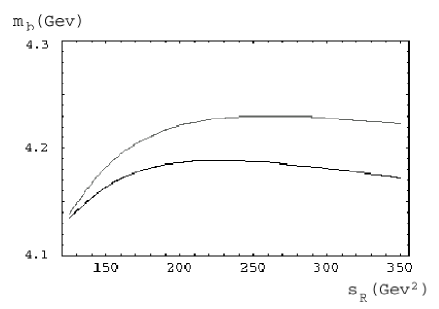
Figure 1: Stability of the two (upper curve) and three (lower curve) loop calculations of the bottom quark mass.

As a sample calculation, we have plotted in figure 1 the results of $m_{b}^{(1,2)}(m_{b})$ as function of the radius $s_{R}$. The upper (lower) curve corresponds to the first (second) order in the strong coupling constant. We find the most stable result for $s_{R}=240\,\,\mathrm{GeV}^{2}$ . The difference between second and first order results is $\varepsilon_{\mathrm{ASY}}=0.04\,\,\mathrm{GeV}$. The $s_{R}$ dependence is so tiny that all the values for the mass in the whole range $\left[150,350\right]\,\,\mathrm{GeV}^{2}$ lie within the relatively small asymptotic error bar.

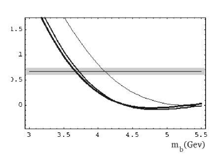
Figure 2: Results for one (thin), two (medium) and three (thick) loops running bottom masses at the renormalization and stability scale $\mu^{2}=s_{R}=240\,\,\mathrm{GeV}^{2}$.

In figure 2 we have plotted the right hand side of the mass equation (5) as a function of $m_{b}(\mu)$ with the renormalization point taken at the value of $s_{R}$ and the latter in the stability point ($\mu^{2}=s_{R}=240\,\,\mathrm{GeV}^{2}$). The thin curve includes only the calculation to one loop, whereas the medium and thick curves include calculations to two and three loops, respectively. The straight strip corresponds to the contribution of the experimental data to the left hand side of equation (5) including experimental error bars. Hence, the crossing of the straight strip with the three curves gives the solution of equation (5), i.e. the results for the running mass $m_{b}^{(0,1,2)}(240\,\,\mathrm{GeV^{2}})$. Running this results to $\mu=m_{b}$ we find the values quoted in equation (8). Notice the very good convergence of the perturbative series at the energies relevant to this process.

4 Conclusions

The bottom quarks mass has been determined in an unconventional fashion by employing finite energy QCD sum rules with positive moments. By  applying Cauchy’s theorem to the $b\overline{b}$ vector current correlator weighted with a real polynomial, it was possible to virtually eliminate the contribution of the yet unknown experimental data in the continuum region from just above the resonances to the beginning of the asymptotic region where QCD is valid. The experimental input needed is only the resonance masses and couplings.

The method we use is quite independent of the more popular one based on inverse moment sum rules. The result we obtain, $m_{b}(m_{b})=(4.19\pm 0.05)\,\,\mathrm{GeV}$, agrees with most of the recent calculations [13], especially with references [8] and [9] that study high and low inverse moment sum rules, respectively. The errors of our calculation are comparable to the ones quoted in these references. Such independent determinations of the same quantity serves as a probe of the validity of the concept of duality which are at the basis of most calculations in the b-sector. We find nice convergence of our result with respect to QCD perturbation theory and negligible non-perturbative contributions.

References

- [1] L. J. Reinders, Phys. Rev. D38 (1988) 947.
- [2] S. Narison, Phys.Lett. B341 (1994) 73.
- [3] M. B. Voloshin, Int. J. Mod. Phys. A10 (1995) 2865.
- [4] A. A. Penin and A.A. Pivovarov, Phys. Lett. B435 (1998) 413; Nucl. Phys. B549 (1999) 217. J. H. Kuhn, A. A. Penin and A.A. Pivovarov, Nucl. Phys. B534 (1998) 356.
- [5] A. H. Hoang, Phys. Rev. D59 (1999) 014039; Phys. Rev. D61 (2000) 034005.
- [6] M. Beneke and A. Signer, Phys. Lett. B471 (1999) 233.
- [7] G. Rodrigo, A. Santamaria and M. S. Bilenky, Phys. Rev. Lett. 79 (1997) 193.
- [8] M. Jamin and A. Pich, Nucl. Phys. Proc. Suppl. 74 (1999) 300; Nucl. Phys. B507 (1997) 334.
- [9] J. H. Kühn and M. Steinhauser, Nucl. Phys. B619 (2001) 588.
- [10] A. Pineda and F. J. Yndurain, Phys. Rev. D58 (1998) 094022; Phys. Rev.D61 (2000) 077505. A. Pineda, Nucl. Phys. B494 (1997) 213.
- [11] V. Giménez et al., Nucl. Phys. Suppl. 83 (2000) 286, JHEP 0003 (2000) 018. C. T. H. Davies et al., Phys. Rev. Lett. 73 (1994) 2654. A. Alikhan et al., Phys. Rev. D62 (2000) 054505.
- [12] S. Narison and E. de Rafael. Nucl. Phys. B169 (1980) 253.
- [13] A. H. Hoang, hep-ph/0204299.
- [14] K. G. Chetyrkin, R. Harlander, J. H. Kühn and M. Steinhauser, Nucl.Phys. B503 (1997) 339.
- [15] K. G. Chetyrkin, R. V. Harlander and J. H. Kühn, Nucl.Phys. B586 (2000)56.
- [16] S. Groote, J. G. Körner, K. Schilcher, N. F. Nasrallah, Phys.Lett. B440 (1998) 375.
- [17] J. Peñarrocha and K. Schilcher. Phys. Lett B515 (2001) 291.
- [18] J. Z. Bai et al. (BES collaboration), Phys. Rev. Lett. 88 (2002) 101802.
- [19] D. J. Broadhurst, P.A. Baikov, J. Fleischer, O. V. Tarasov and V. A. Smirnov, Phys.Lett. B329 (1994) 103.
- [20] N. A. Papadopoulos, J. A. Peñarrocha, F. Scheck and K. Schilcher, Nucl.Phys. B258 (1985) 1.
- [21] G. Rodrigo, A. Pich and A. Santamaria, Phys.Lett. B424 (1998) 367.
- [22] J. A. M. Vermaseren, S. A. Larin and T. van Ritbergen, Phys.Lett. B405 (1997) 327.
- [23] K. Hagiwara et al. (PDG) Phys. Rev. D66 (2002) 010001.
- [24] H. Albrech (ARGUS collaboration), Z. Phys. C65 (1995) 619.
- [25] G. Corcella, A.H. Hoang, Phys.Lett.B554133 (2003).