The analysis of $B_{d}\rightarrow(\eta,\eta^{\prime})\ell^{+}\ell^{-}$ decays in the standard model

Abstract

We study the differential branching ratio, branching ratio and the CP-violating asymmetry for the exclusive $B_{d}\rightarrow(\eta,\eta^{\prime})\ell^{+}\ell^{-}$ decays in the standard model. We deduce the $B_{d}\rightarrow(\eta,\eta^{\prime})$ form factors from the form factors of $B\rightarrow\pi$ available in the literature, by using the $SU(3)_{F}$ symmetry. We observe that these decay modes, which are within the reach of forthcoming B-factories, are very promising to observe CP-violation.

1 Introduction

The decays of B-meson are very promising for investigating the Standard Model (SM) and searching for the new physics beyond it. Among these B-decays, the rare semileptonic ones have attracted much attention for a long time, since they offer the most direct methods to determine the weak mixing angles and Cabibbo-Kobayashi-Maskawa (CKM) matrix elements. These decays can also be very useful to test the various new physics scenarios like the two Higgs doublet models (2HDM), minimal supersymmetric standard model (MSSM)[1]. etc.

From the experimental side, there is an impressive effort to search for B-decays, in B-factories such as Belle, BaBar, LHC-B. For example, CLEO Collaboration reports for the branching ratios $(BRs)$ of the $B^{0}\rightarrow\pi^{-}\ell^{+}\nu$ and $B^{0}\rightarrow\rho^{-}\ell^{+}\nu$ decays [2] as

$$BR(B^{0}\rightarrow\pi^{-}\ell^{+}\nu) = (1.8\pm 0.4\pm 0.3\pm 0.2)\times 10^{-4}$$

$$BR(B^{0}\rightarrow\rho^{-}\ell^{+}\nu) = (2.57\pm 0.29_{-0.46}^{+0.33}\pm 0.41)\times 10^{-4}.$$ (1)

From these results, the value of the CKM matrix element $|V_{ub}|=3.25\pm 0.14^{+0.21}_{-0.29}\pm 0.55$ has been determined [2]. Recently, the BR of the inclusive $B\rightarrow X_{s}\ell^{+}\ell^{-}$ decay has been also reported by Belle Collaboration [3];

$$BR(B\rightarrow X_{s}\ell^{+}\ell^{-})=(6.1\pm 1.4^{+1.4}_{-1.1})\times 10^{-6}\,,$$ (2)

which is very close to the value predicted by the SM [4].

In this paper, we investigate the $B_{d}\rightarrow\,\,{\eta^{(\prime)}}\,\,\ell^{+}\ell^{-}$decay modes within the SM. It is well known that the inclusive rare decays are more difficult to measure, although they are theoretically cleaner than the exclusive ones. This motivates the study of exclusive decays, but their theoretical investigation requires the additional knowledge of decay form factors, i.e. the matrix elements of the effective Hamiltonian between initial B and the final meson states. The nonperturbative sector of QCD is used in order to determine these form factors. Two of the form factors, $f_{+}$ and $f_{-}$, necessary for $B_{d}\rightarrow\,\,\eta\,\,\ell^{+}\ell^{-}$decay have been calculated very recently, in the framework of light-cone QCD sum rules [5]. However, we do not have a precise calculation on the remaining form factor, $f_{T}$ for $B_{d}\rightarrow\,\,{\eta^{(\prime)}}\,\,\ell^{+}\ell^{-}$decay yet. Therefore, in this work, we choose to deduce the form factors of $B_{d}\rightarrow\eta^{(\prime)}$ transition from the form factors of $B\rightarrow\pi$ using the $SU(3)_{F}$ symmetry. The form factors of $B\rightarrow\pi$ have been calculated in the light-cone constituent quark model (LCQM) [6, 7] and also in the QCD sum rules method (QCDSR) [8]; and in this paper, we will give our numerical results using both of these approaches. Let us mension that the $B\rightarrow K$ hadronic matrix elements computed in LCQM and QCDSR have been used to evaluate the semileptonic rate of the $B\rightarrow K\ell^{+}\ell^{-}$ decay mode [9, 10]. Compared to the recently measured value of $BR(B\rightarrow K\ell^{+}\ell^{-})=(0.75^{+0.25}_{-0.21}\pm 0.09)\times 10^{-6}$ by Belle Collaboration [11] and also BaBar Collaboration [12], we see that QCDSR predicts a better result.

In this work, we also calculate the CP asymmetry in the $B_{d}\rightarrow\,\,{\eta^{(\prime)}}\,\,\ell^{+}\ell^{-}$decay, which is induced by the $b\rightarrow d\ell^{+}\ell^{-}$transition at the quark level. For $b\rightarrow s\ell^{+}\ell^{-}$ transition, the matrix element contains the terms that receive contributions from $t\bar{t}$, $c\bar{c}$ and $u\bar{u}$ loops, which are proportional to the combination of $\xi_{t}=V_{tb}V^{*}_{ts}$, $\xi_{c}=V_{cb}V^{*}_{cs}$ and $\xi_{u}=V_{ub}V^{*}_{us}$, respectively. Smallness of $\xi_{u}$ in comparison with $\xi_{c}$ and $\xi_{t}$, together with the unitarity of the CKM matrix elements, bring about the consequence that matrix element for the $b\rightarrow s\ell^{+}\ell^{-}$ decay involves only one independent CKM factor $\xi_{t}$, so that the CP violation in this channel is suppressed in the SM [13, 14]. However, for $b\rightarrow d\ell^{+}\ell^{-}$ decay, all the CKM factors $\eta_{t}=V_{tb}V^{*}_{td}$, $\eta_{c}=V_{cb}V^{*}_{cd}$ and $\eta_{u}=V_{ub}V^{*}_{ud}$ are at the same order in the SM so that they can induce a CP violating asymmetry between the decay rates of the reactions $b\rightarrow d\ell^{+}\ell^{-}$ and $\bar{b}\rightarrow\bar{d}\ell^{+}\ell^{-}$ [15]. So, $b\rightarrow d\ell^{+}\ell^{-}$ decay seems to be suitable for establishing CP violation in B mesons. On the other hand, it should be noted that the detection of the $b\rightarrow d\ell^{+}\ell^{-}$ decay will probably be more difficult in the presence of a much stronger decay $b\rightarrow s\ell^{+}\ell^{-}$ and this would make the corresponding exclusive decay channels more preferable in search of CP violation. In this context, the exclusive $B_{d}\rightarrow(\pi,\rho)\,\ell^{+}\ell^{-}$, and $B_{d}\rightarrow\gamma\,\ell^{+}\ell^{-}$ decays have been extensively studied in the SM [16, 17] and beyond [18]-[22].

The paper is organized as follows: In section 2, first the effective Hamiltonian is presented and the form factors are defined. Then, the basic formulas of the differential branching ratio dBR/ds, branching ratio $BR$ and the CP violating asymmetry $A_{CP}$ for $B_{d}\rightarrow\,\,{\eta^{(\prime)}}\,\,\ell^{+}\ell^{-}$decays are introduced. Section 3 is devoted to the numerical analysis and discussion.

2 Effective Hamiltonian and Form Factors

The leading order QCD corrected effective Hamiltonian, which is induced by the corresponding quark level process $b\rightarrow d\,\ell^{+}\ell^{-}$, is given by [23]-[26]:

$${\cal H}_{eff}=\frac{4G_{F}}{\sqrt{2}}\,V_{tb}V^{*}_{td}\Bigg{\{}\sum_{i=1}^{10} \,\,C_{i}(\mu)\,O_{i}(\mu)-\lambda_{u}\{C_{1}(\mu)[O_{1}^{u}(\mu)-O_{1}(\mu)]$$ (3)

$$+C_{2}(\mu)[O_{2}^{u}(\mu)-O_{2}(\mu)]\}\Bigg{\}}$$

where

$$\lambda_{u}=\frac{V_{ub}V_{ud}^{\ast}}{V_{tb}V_{td}^{\ast}},$$ (4)

using the unitarity of the CKM matrix i.e. $V_{tb}V_{td}^{\ast}+V_{ub}V_{ud}^{\ast}=-V_{cb}V_{cd}^{\ast}$. The explicit forms of the operators $O_{i}$ can be found in refs. [23, 24]. In Eq.(3), $C_{i}(\mu)$ are the Wilson coefficients calculated at a renormalization point $\mu$ and their evolution from the higher scale $\mu=m_{W}$ down to the low-energy scale $\mu=m_{b}$ is described by the renormalization group equation. For $C^{eff}_{7}(\mu)$ this calculation is performed in refs.[27, 28] upto next to leading order. The value of $C_{10}(m_{b})$ to the leading logarithmic approximation can be found e.g. in [23, 26]. The terms that are the source of the CP violation are given by the following, which have a perturbative part and a part coming from long distance (LD) effects due to conversion of the real $\bar{c}c$ into lepton pair $\ell^{+}\ell^{-}$:

$$C_{9}^{eff}(\mu)=C_{9}^{pert}(\mu)+Y_{reson}(s)\,\,,$$ (5)

where

$$C_{9}^{pert}(\mu) = C_{9}+h(u,s)[3C_{1}(\mu)+C_{2}(\mu)+3C_{3}(\mu)+C_{4}(\mu)+3C_{5}(\mu)+C_{6}(\mu)$$

$$+ \lambda_{u}(3C_{1}+C_{2})]-\frac{1}{2}h(1,s)\left(4C_{3}(\mu)+4C_{4}(\mu)+3C_{5}(\mu)+C_{6}(\mu)\right)$$

$$- \frac{1}{2}h(0,s)\left[C_{3}(\mu)+3C_{4}(\mu)+\lambda_{u}(6C_{1}(\mu)+2C_{2}(\mu))\right]$$

$$+ \frac{2}{9}\left(3C_{3}(\mu)+C_{4}(\mu)+3C_{5}(\mu)+C_{6}(\mu)\right)\,\,,$$

and

$$Y_{reson}(s) = -\frac{3}{\alpha^{2}_{em}}\kappa\sum_{V_{i}=\psi_{i}}\frac{\pi\Gamma(V_{i}\rightarrow\ell^{+}\ell^{-})m_{V_{i}}}{m_{B}^{2}s-m_{V_{i}}+im_{V_{i}}\Gamma_{V_{i}}}$$ (7)

$$\times [(3C_{1}(\mu)+C_{2}(\mu)+3C_{3}(\mu)+C_{4}(\mu)+3C_{5}(\mu)+C_{6}(\mu))$$

$$+ \lambda_{u}(3C_{1}(\mu)+C_{2}(\mu))]\,.$$

In Eq.(2), $s=q^{2}/m_{B}^{2}$ where $q$ is the momentum transfer, $u=\frac{m_{c}}{m_{b}}$ and the functions $h(u,s)$ arise from one loop contributions of the four-quark operators $O_{1}-O_{6}$ and are given by

$$h(u,s) = -\frac{8}{9}\ln\frac{m_{b}}{\mu}-\frac{8}{9}\ln u+\frac{8}{27}+\frac{4}{9}y$$ (10)

$$-\frac{2}{9}(2+y)|1-y|^{1/2}\left\{\begin{array}[]{ll}\left(\ln\left|\frac{\sqrt{1-y}+1}{\sqrt{1-y}-1}\right|-i\pi\right),&\mbox{for }y\equiv\frac{4u^{2}}{s}<1\\ 2\arctan\frac{1}{\sqrt{y-1}},&\mbox{for }y\equiv\frac{4u^{2}}{s}>1,\end{array}\right.$$

$$h(0,s) = \frac{8}{27}-\frac{8}{9}\ln\frac{m_{b}}{\mu}-\frac{4}{9}\ln s+\frac{4}{9}i\pi\,\,.$$ (11)

The phenomenological parameter $\kappa$ in Eq. (7) is taken as $2.3$ (see e.g., [15]).

Neglecting the mass of the $d$ quark, the effective short distance Hamiltonian for the $b\rightarrow d\ell^{+}\ell^{-}$ decay in Eq.(3) leads to the QCD corrected matrix element:

$${\cal M} = \frac{G_{F}\alpha}{2\sqrt{2}\pi}V_{tb}V_{td}^{\ast}\Bigg{\{}C_{9}^{eff}(m_{b})~{}\bar{d}\gamma_{\mu}(1-\gamma_{5})b\,\bar{\ell}\gamma^{\mu}\ell+C_{10}(m_{b})~{}\bar{d}\gamma_{\mu}(1-\gamma_{5})b\,\bar{\ell}\gamma^{\mu}\gamma_{5}\ell$$

$$- 2C_{7}^{eff}(m_{b})~{}\frac{m_{b}}{q^{2}}\bar{d}i\sigma_{\mu\nu}q^{\nu}(1+\gamma_{5})b\,\bar{\ell}\gamma^{\mu}\ell\Bigg{\}}.$$

Next we proceed to calculate the $BR$s of the $B_{d}\rightarrow\,\,{\eta^{(\prime)}}\,\,\ell^{+}\ell^{-}$decays. The necessary matrix elements to do this are $<{{\eta^{(\prime)}}}(p_{{\eta^{(\prime)}}})|\bar{d}\gamma_{\mu}(1-\gamma_{5})b|B(p_{B})>$, $<{{\eta^{(\prime)}}}(p_{{\eta^{(\prime)}}})|\bar{d}i\sigma_{\mu\nu}q_{\nu}(1+\gamma_{5})b|B(p_{B})>$ and $<{{\eta^{(\prime)}}}(p_{{\eta^{(\prime)}}})|\bar{d}(1+\gamma_{5})b|B(p_{B})>$. The first two of these matrix elements can be written in terms of the form factors in the following way

$$<{{\eta^{(\prime)}}}(p_{{\eta^{(\prime)}}})|\bar{d}\gamma_{\mu}(1-\gamma_{5})b|B(p_{B})> = f^{+}(q^{2})(p_{B}+p_{{\eta^{(\prime)}}})_{\mu}+f^{-}(q^{2})q_{\mu}\,,$$ (13)

$$<{{\eta^{(\prime)}}}(p_{{\eta^{(\prime)}}})|\bar{d}i\sigma_{\mu\nu}q^{\nu}(1+\gamma_{5})b|B(p_{B})> \!\!\!=\!\!\! [(p_{B}+p_{\eta^{(\prime)}})_{\mu}q^{2}-q_{\mu}(m_{B}^{2}-{m_{\eta^{(\prime)}}}^{2})]f_{v}(q^{2})\,,$$ (14)

where $p_{B}$ and $p_{{\eta^{(\prime)}}}$ denote the four momentum vectors of $B$ and ${\eta^{(\prime)}}$-mesons, respectively. $f_{v}(q^{2})$ is sometimes written as $f_{v}(q^{2})=f_{T}/(m_{B}+m_{\eta^{(\prime)}}^{2})$.

To find $<{{\eta^{(\prime)}}}(p_{{\eta^{(\prime)}}})|\bar{d}(1+\gamma_{5})b|B(p_{B})>$, we multiply both sides of Eq. (13) with $q_{\mu}$ and then use the equation of motion. Neglecting the mass of the $d$-quark, we get

$$<{{\eta^{(\prime)}}}(p_{\eta^{(\prime)}})|\bar{d}(1+\gamma_{5})b|B(p_{B})>=\frac{1}{m_{b}}[f^{+}(q^{2})(m_{B}^{2}-{m_{{\eta^{(\prime)}}}}^{2})+f^{-}(q^{2})q^{2}].$$ (15)

As pointed out in sec.1, although the form factors $f_{+}$ and $f_{-}$ for $B\rightarrow\eta$ decay have been calculated in the framework of the light-cone QCD sum rules in [5], we do not have a precise calculation of the other form factor $f_{v}$ in the literature yet. However, the form factors of $B_{d}\rightarrow\eta^{(\prime)}$ transition can be related to those of $B\rightarrow\pi$ through the $SU(3)_{F}$ symmetry [29, 30]. In addition, the authors of [5] emphasize that, their results coincide with the ones that are calculated using the $SU(3)_{F}$ symmetry. Therefore, we choose to deduce the form factors necessary in this work from the $B\rightarrow\pi$ transition using the $SU(3)_{F}$ symmetry. For $\eta-\eta^{\prime}$ mixing, we adopt the following scheme [31, 32],

$$|\eta> = \cos\,\phi|\eta_{q}>\,-\,\sin\,\phi|\eta_{s}>,$$

$$|\eta^{\prime}> = \sin\,\phi|\eta_{q}>\,+\,\cos\,\phi|\eta_{s}>,$$ (16)

where $|\eta_{q}>=(u\bar{u}+d\bar{d})/\sqrt{2}$, $|\eta_{s}>=s\bar{s}$, and $\phi=39.3$ is the fitted mixing angle [31]. Hence, the relation between the form factors are written as follows:

$$F^{B_{d}\rightarrow\eta}(q^{2}) = \cos\,\phi\,F^{B\rightarrow\pi}(q^{2}),$$

$$F^{B_{d}\rightarrow\eta^{\prime}}(q^{2}) = \sin\,\phi\,F^{B\rightarrow\pi}(q^{2}).$$ (17)

For $B\rightarrow\pi$, we use the results calculated in two different frameworks: In the LCQM, the form factors are parametrized in the following pole forms [6, 7]

$$f^{+}(q^{2}) = \frac{0.29}{\left(1-\frac{q^{2}}{6.71^{2}}\right)^{2.35}}~{},f^{-}(q^{2})=-\frac{0.26}{\left(1-\frac{q^{2}}{6.553^{2}}\right)^{2.30}}~{},$$

$$f_{v}(q^{2}) = -\frac{0.05}{\left(1-\frac{q^{2}}{6.68}\right)^{2.31}}~{}.$$ (18)

However in the QCDSR approach, they are given by [8]

$$f^{+}(q^{2}) = \frac{0.305}{\left(1-1.29\frac{q^{2}}{m_{B}^{2}}+0.206(\frac{q^{2}}{m_{B}^{2}})^{2}\right)}~{},f_{0}(q^{2})=\frac{0.305}{\left(1-0.266\frac{q^{2}}{m_{B}^{2}}-0.752(\frac{q^{2}}{m_{B}^{2}})^{2}\right)}~{},$$

$$f_{T}(q^{2}) = \frac{0.296}{\left(1-1.28\frac{q^{2}}{m_{B}^{2}}+0.193(\frac{q^{2}}{m_{B}^{2}})^{2}\right)}~{},$$ (19)

from which $f^{-}$ can be calculated through the relation:

$$f^{-}=(m_{B}^{2}-m_{\eta^{(\prime)}}^{2})(f_{0}-f^{+})/q^{2}.$$ (20)

Using the above matrix elements, we find the amplitudes governing the $B_{d}\rightarrow\,\,{\eta^{(\prime)}}\,\,\ell^{+}\ell^{-}$decays as follows:

$$\cal{M}^{B\rightarrow\eta^{(\prime)}} = \frac{G_{F}\alpha}{2\sqrt{2}\pi}V_{tb}V_{td}^{\ast}\Bigg{\{}[2Ap_{{{\eta^{(\prime)}}}}^{\mu}+Bq^{\mu}]\bar{\ell}\gamma_{\mu}\ell+[2Gp_{{{\eta^{(\prime)}}}}^{\mu}+Dq^{\mu}]\bar{\ell}\gamma_{\mu}\gamma_{5}\ell\Bigg{\}}~{},$$

where

$$A = C^{eff}_{9}f^{+}-2m_{B}C^{eff}_{7}f_{v},$$

$$B = C^{eff}_{9}(f^{+}+f^{-})+2C^{eff}_{7}\frac{m_{B}}{q^{2}}f_{v}(m_{B}^{2}-m_{{{\eta^{(\prime)}}}}^{2}-q^{2}),$$

$$G = C_{10}f^{+},$$

$$D = C_{10}(f^{+}+f^{-}).$$ (22)

Using Eq.(2) and performing summation over final lepton polarization, we get for the double differential decay rates:

$$\frac{d^{2}\Gamma^{B\rightarrow{{\eta^{(\prime)}}}}}{ds~{}dz} = \frac{G_{F}^{2}\alpha^{2}}{2^{11}\pi^{5}}|V_{tb}V_{td}^{\ast}|^{2}m_{B}^{3}\sqrt{\lambda}~{}v~{}\Bigg{\{}m_{B}^{2}\lambda(1-z^{2}v^{2})|A|^{2}$$ (23)

$$+ (m_{B}^{2}\lambda(1-z^{2}v^{2})+16~{}r~{}m^{2}_{\ell})~{}|G|^{2}+4~{}s~{}m_{\ell}^{2}~{}|D|^{2}$$

$$+ 4~{}m_{\ell}^{2}~{}(1-r-s)~{}Re[G\,D^{\ast}]\Bigg{\}}\,,$$

Here $s=q^{2}/m_{B}^{2}$, $r=m_{{{\eta^{(\prime)}}}}^{2}/m_{B}^{2}$, $v=\sqrt{1-\frac{4t^{2}}{s}}$, $t=m_{\ell}^{2}/m_{B}^{2}$, $\lambda=r^{2}+(s-1)^{2}-2r(s+1)$, and $z=\cos\theta$, where $\theta$ is the angle between the three-momentum of the $\ell^{-}$ lepton and that of the B-meson in the center of mass frame of the dileptons $\ell^{+}\ell^{-}$. After integrating over the angle variable we find

$$\frac{d\Gamma^{B\rightarrow{{\eta^{(\prime)}}}}}{ds} = \frac{G_{F}^{2}\alpha^{2}}{2^{10}\pi^{5}}|V_{tb}V_{td}^{\ast}|^{2}m_{B}^{3}\sqrt{\lambda}\,v\,\Delta\,,$$ (24)

where

$$\Delta = \frac{1}{3}~{}m_{B}^{2}~{}\lambda(3-v^{2})(|A|^{2}+|G|^{2})+\frac{4m_{\ell}^{2}}{3s}(12\,r~{}s+\lambda)|G|^{2}$$ (25)

$$+ 4~{}m_{\ell}^{2}~{}s~{}|D|^{2}+4~{}m_{\ell}^{2}(1-r-s)Re[G~{}D^{\ast}]\,.$$

We now consider the CP violating asymmetry, $A_{CP}$, between the $B_{d}\rightarrow\,\,{\eta^{(\prime)}}\,\,\ell^{+}\ell^{-}$and $\overline{B}_{d}\rightarrow\,\,\overline{\eta}^{(\prime)}\,\,\ell^{+}\ell^{-}$ decays, which is defined as follows:

$$A_{CP}(x)=\frac{\Gamma(B_{d}\rightarrow\,\,\eta^{(\prime)}\,\,\ell^{+}\ell^{-})-\Gamma(\overline{B}_{d}\rightarrow\,\,\overline{\eta}^{(\prime)}\,\,\ell^{+}\ell^{-})}{\Gamma(B_{d}\rightarrow\,\,{{\eta^{(\prime)}}}\,\,\ell^{+}\ell^{-})+\Gamma(\overline{B}_{d}\rightarrow\,\,\overline{\eta}^{(\prime)}\,\,\ell^{+}\ell^{-})}~{}~{}.$$ (26)

Using this definition we calculate the $A_{CP}$ as:

$$A_{CP}=\frac{\int H(s)~{}ds}{\int(\Delta-H(s))~{}ds},$$ (27)

where

$$H(s) = \frac{2}{3}\,f_{+}m_{B}^{2}(3-\upsilon^{2})\lambda~{}Im~{}\lambda_{u}~{}\Bigg{(}Im~{}\xi_{2}~{}C_{7}^{eff}~{}f_{T}\frac{2m_{b}}{m_{B}+m_{{{\eta^{(\prime)}}}}}-f_{+}~{}(Im~{}\xi_{1}^{\ast}~{}\xi_{2})\Bigg{)}.$$ (28)

In calculating this expression, we use the following parametrizations:

$$C_{9}^{eff}\equiv\xi_{1}+\lambda_{u}~{}\xi_{2}\,,$$ (29)

$$\lambda_{u}=\frac{\rho(1-\rho)-\eta^{2}-i\eta}{(1-\rho)^{2}+\eta^{2}}+O(\lambda^{2}).$$ (30)

3 Numerical Results and Discussion

In this section we present the numerical results of our calculations related to $B_{d}\rightarrow\,\,{\eta^{(\prime)}}\,\,\ell^{+}\ell^{-}$$(\ell=e,\,\mu,\,\tau)$ decays, for four different sets of parameter choice of the form factors and the updated fits of the Wolfenstein parameters [33], which are summarized in Table 1. The total $BR$s are collected in Table 2. We have also evaluated the average values of CP asymmetry $<A_{CP}>$ in $B_{d}\rightarrow\,\,{\eta^{(\prime)}}\,\,\ell^{+}\ell^{-}$decays for the above sets of parameters, and our results are displayed in Table 3. In both tables, the values in the paranthesis are the corresponding quantities calculated without including the long distance effects. We observe that the results of $<A_{CP}>$ is very sensitive to the choice of four different sets of parameters for $\tau$ channel, while they are very close to each other for $\mu$ channel.

	$(\rho;\eta)$	Form   factors
set-1	$(0.3;0.34)$	LCQM
set-2	$(0.15;0.34)$	LCQM
set-3	$(0.3;0.34)$	QCDSR
set-4	$(0.15;0.34)$	QCDSR

Table 1: List of the values for the Wolfenstein parameters and the form factors of the transition $B\rightarrow\pi$ calculated in the light-cone constituent quark model (LCQM) [6, 7] and light-cone QCD sum rule approach (QCDSR) [8].

The input parameters and the initial values of the Wilson coefficients we used in our numerical analysis are as follows:

$$m_{B}=5.28\,GeV\,,\,m_{b}=4.8\,GeV\,,\,m_{c}=1.4\,GeV\,,m_{\tau}=1.78\,GeV,\,$$

$$m_{\mu}=0.105\,GeV,\,\left|V_{tb}V_{td}^{\ast}\right|=0.01,\,m_{\eta}=0.547\,GeV,\,m_{\eta^{\prime}}=0.958\,GeV,\,$$

$$C_{1}=-0.245,\,C_{2}=1.107,\,C_{3}=0.011,\,C_{4}=-0.026,\,C_{5}=0.007,\,$$

$$C_{6}=-0.0314,\,C^{eff}_{7}=-0.315,\,C_{9}=4.220,\,C_{10}=-4.619.$$ (31)

There are five possible resonances in the $c\bar{c}$ system that can contribute to the decay under consideration and to calculate their contributions, we need to divide the integration region for $s$ into three parts for $\ell=e,\mu$ so that we have $4m^{2}_{\ell}/m_{B}^{2}\leq s\leq(m_{\psi_{1}}-0.02)^{2}/m_{B}^{2}$ and $(m_{\psi_{1}}+0.02)^{2}/m_{B}^{2}\leq s\leq(m_{\psi_{2}}-0.02)^{2}/m_{B}^{2}$ and $(m_{\psi_{2}}+0.02)^{2}/m_{B}^{2}\leq s\leq(m_{B}-m_{\eta^{(\prime)}})^{2}/m_{B}^{2}$, while for $\ell=\tau$ it takes the form given by $4m^{2}_{\tau}/m_{B}^{2}\leq s\leq(m_{\psi_{2}}-0.02)^{2}/m_{B}^{2}$ and $(m_{\psi_{2}}+0.02)^{2}/m_{B}^{2}\leq s\leq(m_{B}-m_{\eta^{(\prime)}})^{2}/m_{B}^{2}$ . Here, $m_{\psi_{1}}$ and $m_{\psi_{2}}$ are the masses of the first and the second resonances, respectively.

$10^{8}\cdot BR$	$\ell$	set1	set2	set3	set4
	$\tau$	$0.331$	$0.313$	$0.687$	$0.659$
		$(0.324)$	$(0.314)$	$(0.695)$	$(0.677)$
$\eta$	$\mu$	$2.704$	$2.511$	$3.704$	$3.468$
		$(2.119)$	$(2.063)$	$(3.049)$	$(2.966)$
	$e$	$2.713$	$2.520$	$3.716$	$3.479$
		$(2.127)$	$(2.371)$	$(3.059)$	$(2.976)$
	$\tau$	$0.092$	$0.087$	$0.153$	$0.146$
		$(0.086)$	$(0.083)$	$(0.147)$	$(0.144)$
$\eta^{\prime}$	$\mu$	$1.363$	$1.268$	$1.779$	$1.666$
		$(1.033)$	$(1.010)$	$(1.395)$	$(1.365)$
	$e$	$1.369$	$1.273$	$1.786$	$1.674$
		$(1.038)$	$(1.015)$	$(1.402)$	$(1.372)$

Table 2: The SM predictions for the integrated branching ratios for $\ell=\tau,\mu,e$ of the $B_{d}\rightarrow\eta^{(\prime)}\ell\ell$ decay with (without) the long-distance effects.

In Fig. (1) and Fig. (2), we present the dependence of the $BR$ on the invariant mass of dileptons, $s$, for the $B_{d}\rightarrow\,\,{\eta}\,\,\tau^{+}\tau^{-}$and $B_{d}\rightarrow\,\,{\eta}\,\,\mu^{+}\mu^{-}$decays, respectively. We plot these graphs for the parameter set-1 and set-3 in Table 1, represented by the dashed and the solid curves, respectively. The sharp peaks in the figures are due to the long distance contributions. As can be seen from these graphs, $BR$ stands more for the parameter set-3. The same analysis above is made for $B_{d}\rightarrow\,\,{\eta^{\prime}}\,\,\tau^{+}\tau^{-}$ and $B_{d}\rightarrow\,\,{\eta^{\prime}}\,\,\mu^{+}\mu^{-}$ decays in Fig. (3) and Fig. (4), respectively.

Figs. (5) and (6) are devoted to the $A_{CP}(s)$ as a function of $s$ for $B_{d}\rightarrow\eta\,\tau^{+}\tau^{-}$ and $B_{d}\rightarrow\eta\,\mu^{+}\mu^{-}$ decays, respectively. In these figures, the small dashed (dotted dashed) and the solid (dashed) curves represent the $A_{CP}(s)$ for the parameter set-1 and set-3 with (without) long distance contributions. The dependence of $A_{CP}$ on $s$ for the $\eta^{\prime}$ channel is plotted in Fig. (7) and Fig. (8), for $\ell=\tau$ and $\ell=\mu$, respectively. We see from these figures that for $\ell=\mu$, $A_{CP}(s)$ is not very sensitive to the choice of the parameters set-1 or set-3, reaching up to $28\%$ for the larger values of $s$ for both the $\eta$ and $\eta^{\prime}$ channels. However for $\ell=\tau$ case, $A_{CP}(s)$ gets slightly larger contribution from set-3 than set-1, but reaches at most $25\%$ in the small-$s$ region. We note that $A_{CP}(s)$ is positive for all values of $s$, except in some resonance regions. We also observe from table 3 that including the long-distance effects in calculating $<A_{CP}>$ changes the results only by $2-10\%$ for $\ell=\mu$ mode, but for $\ell=\tau$, it becomes very sizable, $30-150\%$, depending on the sets of parameters used for $(\rho;\eta)$.

In conclusion, we have analyzed the $B_{d}\rightarrow\,\,{\eta^{(\prime)}}\,\,\ell^{+}\ell^{-}$decays within the SM. We have found that, these decay modes have a significant $A_{CP}$, especially for $\ell=\tau$. Since calculated $BR$s of these decay modes are within the reach of forthcoming B-factories such as LHC-B, where approximately $6\times 10^{11}$ $B_{d}$ mesons are expected to be produced per year, we may hope that it can be measured in near future.

$10\cdot<A_{CP}>$	$\ell$	set1	set2	set3	set4
	$\tau$	$1.291$	$0.961$	$2.271$	$0.840$
		$(0.899)$	$(0.657)$	$(0.897)$	$(0.560)$
$\eta$	$\mu$	$0.647$	$0.496$	$0.692$	$0.526$
		$(0.663)$	$(0.484)$	$(0.671)$	$(0.490)$
	$e$	$0.647$	$0.496$	$0.693$	$0.526$
		$(0.663)$	$(0.484)$	$(0.671)$	$(0.490)$
	$\tau$	$0.926$	$0.693$	$0.886$	$0.656$
		$(0.699)$	$(0.510)$	$(0.629)$	$(0.458)$
$\eta^{\prime}$	$\mu$	$0.578$	$0.444$	$0.593$	$0.452$
		$(0.637)$	$(0.464)$	$(0.639)$	$(0.465)$
	$e$	$0.579$	$0.444$	$0.594$	$0.452$
		$(0.638)$	$(0.464)$	$(0.640)$	$(0.465)$

Table 3: The same as Table (2), but for $<A_{CP}>$.

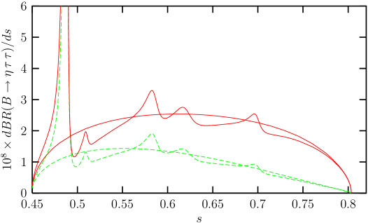
Figure 1: Differential branching ratio for $B\rightarrow\eta\,\tau^{+}\tau^{-}$ decay as a function of $s$ for the parameter set-1 and set-3, represented by the dashed and the solid curves, respectively. The sharp peaks in the figures are due to the long distance contributions.

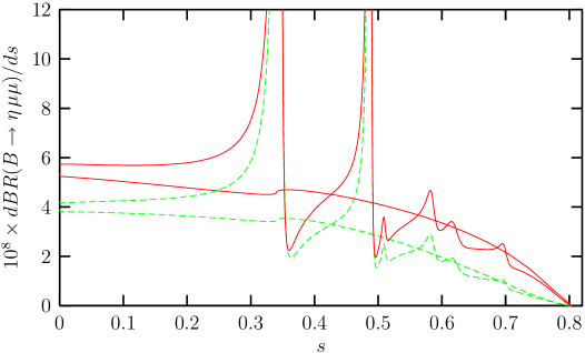
Figure 2: The same as Fig.(1) but for the $B\rightarrow\eta\,\mu^{+}\mu^{-}$ decay

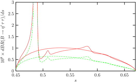
Figure 3: The same as Fig.(1) but for the $B\rightarrow\eta^{\prime}\,\tau^{+}\tau^{-}$ decay

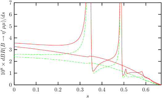
Figure 4: The same as Fig.(1) but for the $B\rightarrow\eta^{\prime}\,\mu^{+}\mu^{-}$ decay

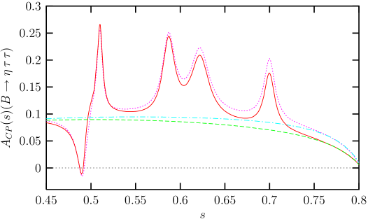
Figure 5: $A_{CP}(s)$ for $B\rightarrow\eta\,\tau^{+}\tau^{-}$ decay for the parameter set-1 and set-3 with (without) long distance contributions, represented by the small dashed (dotted dashed) and the solid (dashed) curves, respectively.

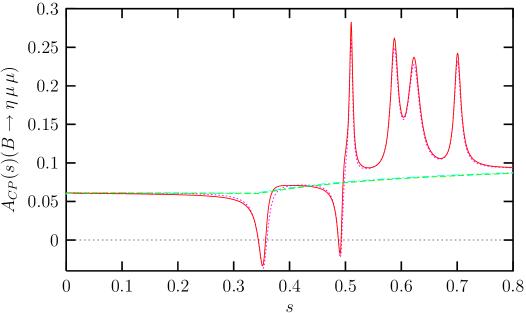
Figure 6: The same as Fig.(5) but for the $B\rightarrow\eta\,\mu^{+}\mu^{-}$ decay

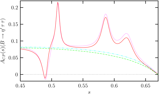
Figure 7: The same as Fig.(5) but for the $B\rightarrow\eta^{\prime}\,\tau^{+}\tau^{-}$ decay

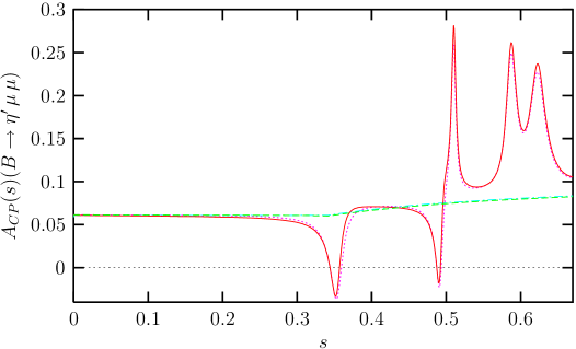
Figure 8: The same as Fig.(5) but for the $B\rightarrow\eta^{\prime}\,\mu^{+}\mu^{-}$ decay