On the Behavior of the Effective QCD
Coupling $\alpha_{\tau}(s)$ at Low Scales

Abstract

The hadronic decays of the $\tau$ lepton can be used to determine the effective charge $\alpha_{\tau}(m^{2}_{\tau^{\prime}})$ for a hypothetical $\tau$-lepton with mass in the range $0<m_{\tau^{\prime}}<m_{\tau}$. This definition provides a fundamental definition of the QCD coupling at low mass scales. We study the behavior of $\alpha_{\tau}$ at low mass scales directly from first principles and without any renormalization-scheme dependence by looking at the experimental data from the OPAL Collaboration. The results are consistent with the freezing of the physical coupling at mass scales $s=m^{2}_{\tau^{\prime}}$ of order $1\,{\rm GeV}^{2}$ with a magnitude $\alpha_{\tau}\sim 0.9\pm 0.1$.

Submitted to Physical Review D

I Introduction

One of the major uncertainties in making reliable predictions in quantum chromodynamics (QCD) is to understand the theory at low momentum scales where the coupling becomes large and non-perturbative effects become important. In fact, it is well known that perturbation theory itself is not well defined in the infrared domain, since the perturbative series is asymptotic. For infrared-safe quantities the non-perturbative effects can be parameterized as power corrections of the form $c_{n}(\Lambda/Q)^{n}$, where $\Lambda$ is the QCD-scale and $Q$ is the hard scale of the process considered. The coefficients $c_{n}$ cannot be calculated in general, but in some cases such as the event-shapes in ${\rm e}^{+}{\rm e}^{-}$ annihilation, one can determine the dominating power $n$ and also find relations between the $c_{n}$ for different observables by using the operator product expansion [1] or renormalon calculus (for a review see ref. [2]).

The behavior of fixed-order perturbation theory at low momentum scales is governed by the running coupling $\alpha_{\rm s}(k^{2})$. The conventional coupling $\alpha_{\hbox{$\overline{\hbox{MS}}$}}(k^{2})$, defined using the modified minimal subtraction renormalization scheme and dimensional regularization, is analytically singular at a scale $k^{2}=\Lambda^{2}_{\hbox{$\overline{\hbox{MS}}$}}$. This nonphysical behavior leads to a number of difficulties, including renormalon $n!$ growth of the coefficients when one makes perturbative expansions of physical observables in the $\overline{\rm MS}$ scheme. These problems can be traced to the fact that integrals over the running coupling which appear in bubble graphs are ill-defined due to the non-analyticity of the $\overline{\rm MS}$ coupling.

There also exists the possibility to define a running coupling which stays finite in the infrared. One such example is the “time-like” effective coupling which is used in the dispersive approach [3, 4, 5]. In this approach, an observable is written as an integral over a process dependent characteristic function times a universal “time-like” effective coupling. The idea is that such a coupling may give an effective measure of the interaction at low scales [5]. Power corrections can then be written as process dependent moments over the effective coupling.

An alternative procedure is to define the fundamental coupling of QCD from a given physical observable [6, 7]. These couplings, called effective charges, are all-order resummations of perturbation theory and include all non-perturbative effects. Since these physical charges correspond to the complete theory of QCD, it is guaranteed that they are analytic and non-singular. For example, it has been shown that unlike the $\overline{\rm MS}$ coupling, a physical coupling is analytic across quark flavor thresholds [8, 9]. Furthermore, we expect that a physical coupling should stay finite in the infrared when the momentum scale goes to zero. In turn, this means that integrals over the running coupling are well defined for physical couplings. An additional question is whether the physical couplings freeze to a constant value in the infrared.

Once such a physical coupling $\alpha_{\rm phys}(k^{2})$ is chosen, other physical quantities can be expressed as expansions in $\alpha_{\rm phys}$ by eliminating the $\overline{\rm MS}$ coupling which now becomes only an intermediary [10]. In such a procedure there are in principle no further renormalization scale ($\mu$) or scheme ambiguities. The physical couplings satisfy the standard renormalization group equation for its logarithmic derivative, ${{\rm d}\alpha_{\rm phys}/{\rm d}\ln k^{2}}=\hat{\beta}_{\rm phys}[\alpha_{\rm phys}(k^{2})]$, where the first two terms in the perturbative expansion of the Gell-Mann Low function $\hat{\beta}_{\rm phys}$ are scheme-independent at leading twist whereas the higher order terms have to be calculated for each observable separately using perturbation theory.

Quantum field theoretic predictions which relate physical observables cannot depend on theoretical conventions such as the choice of renormalization scheme or scale ($\mu$). The most well-known example is the perturbative “generalized Crewther relation” [11] in which the leading twist QCD corrections to the Bjorken sum rule for polarized deep inelastic scattering at a given lepton momentum transfer $Q^{2}$ are related through a geometric series to the QCD corrections to $R_{{\rm e}^{+}{\rm e}^{-}}$ at a corresponding CM energy squared, $s^{*}=s^{*}(Q^{2})$, independent of renormalization scheme, $(1+\alpha_{R}(s^{*})/\pi)(1-\alpha_{g_{1}}(Q^{2})/\pi)=1$ [12]. The ratio of the scales $s^{*}/Q^{2}$ has been computed to NLO in PQCD. Such leading-twist predictions between observables are called “commensurate scale relations” and are identical for conformal and nonconformal theories [10]. In addition, the conformal coefficients are free of the renormalon factorial growth [13, 14, 15]

For example, in QED, the Gell-Mann Low running coupling $\alpha_{\rm QED}(k^{2})={\alpha(k_{0}^{2})\over 1-\Pi(k^{2},k_{0}^{2})}$, which is formally defined from the renormalization of the dressed photon propagator, is a physical coupling since it could be determined from a measurement of the part of the potential $V(k^{2})$ between two infinitely heavy test charges which is linear in their charges; i.e., $4\pi\alpha_{\rm QED}(k^{2})=-k^{2}V_{\rm lin}(k^{2})$. Using the skeleton expansion [16], the coefficients in perturbative expansions of other physical quantities are identical to that in a theory which is conformal, since all effects of the non-zero $\hat{\beta}$ function are already summed into the integrals over the running coupling. By the mean value theorem, the same is also true for the standard perturbative expansion if the scale, at which to evaluate the coupling, is properly chosen [17, 18].

It is not as simple to identify a suitable physical coupling to be used in the case of QCD. For a skeleton expansion to be possible, the Abelian part of the coupling should coincide with the Gell-Mann Low coupling, since QCD becomes an Abelian theory in the analytic limit $N_{\rm c}\to 0$ at fixed $C_{\rm F}\alpha_{\rm s}$ and fixed $n_{\rm f}/C_{\rm F}$ [19]. A possible candidate for a physical coupling in QCD which fulfills this requirement is the $\alpha_{V}(k^{2})$ scheme defined from the potential between two heavy test color charges [20]. However, in contrast to the Abelian case, this definition is problematic since the “$H-$graphs” which arise from gluon exchange diagrams with a horizontal gluon rung connecting the “first” and “last” exchanged gluons have an infrared sensitivity which depends on the details of the test charge wavefunction [21]. Another possible generalization of the Gell-Man Low coupling to non-Abelian theories is the “pinch” scheme [22, 23, 24] which rearranges the contributions to scattering amplitudes to insure a structure $\alpha_{\rm pinch}(k^{2})={\alpha_{\rm pinch}(k_{0}^{2})\over 1-\Pi(k^{2},k_{0}^{2})}$ similar to that of QED. As in QED, expansions in the pinch scheme have the same structure as those of a conformal theory. The pinch charge is a promising physical scheme, but at this time the complexity of higher order calculations in this scheme and its indirect connection to measurements has prevented its practical implementation, although recently there has been attempts to make an all-orders definition of a QCD effective charge [25].

In this note we will discuss an alternative definition of a physical coupling for QCD which has a direct relation to high precision measurements of the hadronic decay channels of the $\tau^{-}\to\nu_{\tau}{\rm h}^{-}$. Details on the extraction of $\alpha_{\rm s}(m_{\tau}^{2})$ from $\tau$ decays can be found in refs. [4, 26, 27, 28, 29, 30, 31, 32, 33, 34, 35] (for some recent developments in the extraction of $\alpha_{\rm s}(m_{\tau}^{2})$ from $\tau$ decays see for example [36, 37, 38, 39]).

Let $R_{\tau}$ be the ratio of the hadronic decay rate to the leptonic one. Then $R_{\tau}\equiv R_{\tau}^{0}\left[1+{\alpha_{\tau}\over\pi}\right]$, where $R_{\tau}^{0}$ is the zeroth order QCD prediction, defines the effective charge $\alpha_{\tau}$. Throughout this paper we will concentrate on non-strange decay modes and thus $R_{\tau}^{0}=3S_{\rm EW}|V_{\rm ud}|^{2}$ where $S_{\rm EW}=1.0194$ is an electroweak correction term [40] and $|V_{\rm ud}|^{2}=0.9512\pm 0.0008$ [41] is the relevant CKM matrix element. The data for $\tau$ decays is well-understood channel by channel, thus allowing a precise separation of vector and axial-vector decay modes which can therefore be studied separately.

The measured invariant mass spectrum for the non-strange hadronic decay modes can also be used to study hypothetical $\tau$-leptons with a smaller mass, $m_{\tau^{\prime}}<m_{\tau}$ [33, 34, 35]. In this way the $\tau$-decay data allows us to study the behavior of the coupling $\alpha_{\tau}(s)$ in the region $0\leq s\leq m_{\tau}^{2}$ and address the question whether this physical coupling freezes in the infrared.

II Extracting $\alpha_{\tau}(s)$ from data on $\tau$-decays

The experimental data on the non-strange hadronic $\tau$-decays can be used to define the hadronic decay rate normalized to the leptonic one for a hypothetical $\tau$-lepton with mass in the range $0<m_{\tau^{\prime}}<m_{\tau}$ in the following way [34]:

$$R_{\tau}^{\rm V/A}(m_{\tau^{\prime}}^{2})\equiv 12\pi S_{\rm EW}|V_{\rm ud}|^{2}\!\!\!\int\limits_{0}^{m_{\tau^{\prime}}^{2}}\!\!\frac{{\rm d}s}{m_{\tau^{\prime}}^{2}}\left(1-\frac{s}{m_{\tau^{\prime}}^{2}}\right)^{2}\left[\left(1+2\frac{s}{m_{\tau^{\prime}}^{2}}\right){\rm Im}\Pi_{\rm V/A}^{(1)}(s)+{\rm Im}\Pi_{\rm V/A}^{(0)}(s)\right],$$ (1)

where $2\pi{\rm Im}\Pi_{\rm V/A}^{(1)}(s)=v/a(s)$ are the spectral functions for the measured non-strange hadronic final states with angular momentum $J=1$. The scalar contribution ${\rm Im}\Pi_{\rm V/A}^{(0)}(s)$ is assumed to vanish for the vector current and is given by the single pion pole for the axial current. The above definition coincides with the standard definition in the case $m_{\tau^{\prime}}=m_{\tau}$. Note, however, that the right-hand side above uses $m_{\tau^{\prime}}$ instead of $m_{\tau}$ not only in the upper integration limit but also in the kinematic prefactors. This way the end-point is suppressed in the same way for the hypothetical $\tau$-lepton as for the real one [34]. The ratio $R_{\tau}^{\rm V/A}(m_{\tau^{\prime}}^{2})$ is thus defined as if a hypothetical lepton of mass $m_{\tau^{\prime}}$ existed.

Since states with non-zero strangeness can be excluded, all of the hadrons in the final state can be assumed to arise from $\tau^{-}\to\nu_{\tau}\bar{\rm u}{\rm d}$. We can then define effective charges $\alpha^{\rm V/A}_{\tau}(m_{\tau^{\prime}}^{2})$ for the vector and axial-vector decay modes as follows:

$$R_{\tau}^{\rm V/A}(m_{\tau^{\prime}}^{2})\equiv\frac{R_{\tau}^{0}}{2}\left[1+{\alpha_{\tau}^{\rm V/A}(m_{\tau^{\prime}}^{2})\over\pi}\right].$$ (2)

Notice that the combination $R_{\tau}^{\rm V}-R_{\tau}^{\rm A}$ does not receive a perturbative QCD contribution at leading twist; thus if QCD is correct this contribution should be power law suppressed at high energies. It is thus natural to identify the complimentary $R_{\tau}^{\rm V}+R_{\tau}^{\rm A}$ combination which has canonical perturbative QCD contributions as the preferred QCD effective charge, $\alpha_{\tau}(m_{\tau^{\prime}}^{2})$, defined by

$$R_{\tau}(m_{\tau^{\prime}}^{2})=R_{\tau}^{\rm V}(m_{\tau^{\prime}}^{2})+R_{\tau}^{\rm A}(m_{\tau^{\prime}}^{2})\equiv R_{\tau}^{0}\left[1+{\alpha_{\tau}(m_{\tau^{\prime}}^{2})\over\pi}\right].$$ (3)

For completeness, we also recall how one can use experimental data to measure the decay ratio of hypothetical $\tau$-leptons for masses well above $m_{\tau}$ [42]. Just as in the case of $\tau$-leptons one can define a local unintegrated effective charge $\alpha_{R}(s)$ directly from the annihilation data:

$$R_{{\rm e}^{+}{\rm e}^{-}}(s)={\sigma({\rm e}^{+}{\rm e}^{-}\to{\rm hadrons})\over\sigma({\rm e}^{+}{\rm e}^{-}\to\mu^{+}\mu^{-})}\equiv R_{{\rm e}^{+}{\rm e}^{-}}^{0}\left[1+\frac{\alpha_{R}(s)}{\pi}\right],$$ (4)

where $R_{{\rm e}^{+}{\rm e}^{-}}^{0}$ is the zeroth order QCD prediction. If we assume isospin invariance, then the decay ratio of a hypothetical $\tau$-lepton in the vector channel $R_{\tau}^{\rm V}(m_{\tau^{\prime}}^{2})$ can be written as a spectral integral with weight $f(x)=\left(1-x\right)^{2}\left(1+2x\right)$, where $x={s/m_{\tau^{\prime}}^{2}}$, of the annihilation cross section ${\rm e}^{+}{\rm e}^{-}\to\gamma^{*}\to{\rm hadrons}$ in the isospin $I=1$ channel. This allows the measurement of $\alpha^{V}_{\tau}(m_{\tau^{\prime}}^{2})$ well above the physical mass of the $\tau$ [42]. We thus can relate the $\alpha^{V}_{\tau}$ and $\alpha_{R}^{(I=1)}$ effective charges:

$$\alpha^{V}_{\tau}(m_{\tau^{\prime}}^{2})={\displaystyle{\int^{m_{\tau^{\prime}}^{2}}_{0}\frac{{\rm d}s}{m_{\tau^{\prime}}^{2}}\,f\left(\frac{s}{m_{\tau^{\prime}}^{2}}\right)\alpha^{(I=1)}_{R}(s)}\over{\displaystyle\int^{m_{\tau^{\prime}}^{2}}_{0}\frac{{\rm d}s}{m_{\tau^{\prime}}^{2}}\,f\left(\frac{s}{m_{\tau^{\prime}}^{2}}\right)}}.$$ (5)

The mean value theorem then implies

$$\alpha^{V}_{\tau}(m_{\tau^{\prime}}^{2})=\alpha^{(I=1)}_{R}(s^{*}),\hskip 56.9055pt0\leq s^{*}\leq m_{\tau^{\prime}}^{2},$$ (6)

a form of commensurate scale relation. In the case of three flavors ($n_{\rm f}=3$) the above relation is still valid to next-to-next-to-leading order even if one does not restrict oneself to the $I=1$ channel. To next-to-leading order in $\alpha_{R}$ the scale $s^{*}$ is given by (see for example [10])

$$s^{*}=m_{\tau^{\prime}}^{2}\exp\left[-{19\over 12}-{169\over 576}\left(11-\frac{2}{3}n_{\rm f}\right)\frac{\alpha_{R}}{\pi}\right].$$ (7)

Before continuing we also note that as an alternative definition of a hypothetical $\tau$-lepton with mass above $m_{\tau}$ one could use ${\rm Im}\Pi_{\rm V}^{(1)}(s)$ measured from $\tau$-decays for the integration region $0<s<m_{\tau}^{2}$ and data from $R_{{\rm e}^{+}{\rm e}^{-}}(s)$ in the $I=1$ channel for the remaining integration region $m_{\tau}^{2}<s<m_{\tau^{\prime}}^{2}$.

The empirical behavior of the decay ratios $R_{\tau}$, $R_{\tau}^{\rm V}$, $R_{\tau}^{\rm A}$, and $R_{\tau}^{\rm V}-R_{\tau}^{\rm A}$ using data on $\tau$-decays as determined by the OPAL collaboration at LEP [35, 43] are shown in fig. 1.

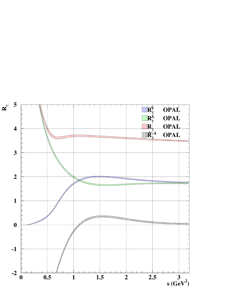
FIG. 1.: The non-strange hadronic decay rate of a hypothetical $\mathit{\tau}$ lepton with $\mathit{m_{\tau^{\prime}}^{2}=s}$ versus the upper integration limit $\mathit{s}$ for the currents $\mathit{V}$, $\mathit{A}$, $\mathit{V+A}$, and $\mathit{V-A}$. Error bands include statistical and systematic errors.

There are several striking features:

1. the $R_{\tau}^{\rm V}-R_{\tau}^{\rm A}$ combination tends to vanish at high scales, showing that only higher dimensional operators contribute. This is a highly non-trivial test of QCD. [44, 45]

2. The $R_{\tau}$ contribution has only a slow variation in the low mass range.

The corresponding effective charges $\alpha_{\tau}$, $\alpha_{\tau}^{\rm V}$, and $\alpha_{\tau}^{\rm A}$ as well as the difference $\alpha_{\tau}^{\rm V}-\alpha_{\tau}^{\rm A}$ are shown in Fig. 2.

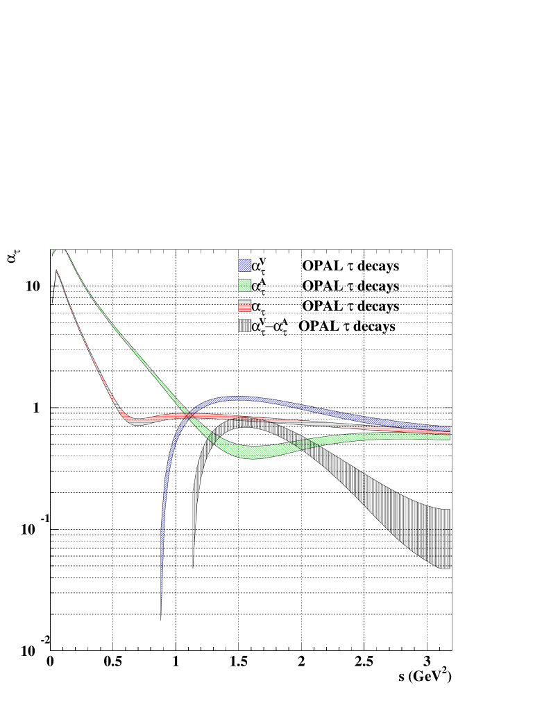
FIG. 2.: The effective charges for non-strange hadronic decays of a hypothetical $\mathit{\tau}$ lepton with $\mathit{m_{\tau^{\prime}}^{2}=s}$ versus the upper integration limit $\mathit{s}$ for the currents $\mathit{V}$, $\mathit{A}$, $\mathit{V+A}$. Also shown is the difference of the effective charges for the vector and axial-vector current. Error bands include statistical and systematic errors.

Based on the analysis by the OPAL collaboration [35], the experimental value of the coupling $\alpha_{\tau}(s)=0.621\pm 0.008$ at $s=m^{2}_{\tau}$ corresponds to a value of $\alpha_{\hbox{$\overline{\hbox{MS}}$}}(M^{2}_{Z})=(0.117$-$0.122)\pm 0.002$, where the range corresponds to three different perturbative methods used in analyzing the data. This result is, at least for the fixed order and renormalon resummation methods, in good agreement with the world average $\alpha_{\hbox{$\overline{\hbox{MS}}$}}(M^{2}_{Z})=0.117\pm 0.002$ [46]. However, from the figure we also see that the effective charge only reaches $\alpha_{\tau}(s)\sim 0.9\pm 0.1$ at $s=1\,{\rm GeV}^{2}$, and it even stays within the same range down to $s\sim 0.5\,{\rm GeV}^{2}$. This result is in good agreement with the estimate of Mattingly and Stevenson [47] for the effective coupling $\alpha_{R}(s)\sim 0.85$ for $\sqrt{s}<0.3\,{\rm GeV}$ determined from ${\rm e}^{+}{\rm e}^{-}$ annihilation, especially if one takes into account the perturbative commensurate scale relation, $\alpha_{\tau}(m_{\tau^{\prime}}^{2})=\alpha_{R}(s^{*})$ where, for $\alpha_{R}=0.85$, we have $s^{*}\simeq 0.10\,m_{\tau^{\prime}}^{2}$ according to Eq. (7). As we will show in more detail in the next section, this behavior is not consistent with the coupling having a Landau pole but rather shows that the physical coupling is much more constant at low scales, suggesting that physical QCD couplings are effectively constant or “frozen” at low scales.

At the same time, it should be recognized that the behavior of $\alpha_{\tau}(s)$ in the region $s<1\,{\rm GeV}^{2}$ is more and more influenced by non-perturbative effects as the scale is lowered. Even though the dominant non-perturbative effects cancel in the sum of the vector and axial-vector contributions as can be seen by looking at the corresponding effective charges individually. Looking at $\alpha_{\tau}^{\rm V}(s)$, we see that it more or less vanishes as the integration region moves to the left of the two-pion peak in the hadronic spectrum. In the same way the behavior of $\alpha_{\tau}^{\rm A}(s)$ at small scales is governed by the single pion pole.

III Analysis of the infrared behavior of $\alpha_{\tau}(s)$

In order to be able to analyze the infrared behavior of the effective coupling $\alpha_{\tau}(s)$ in more detail, we will compare with (a) the fixed-order perturbative evolution of the $\alpha_{\tau}(s)$ coupling on the one hand, and (b) with the evolution of couplings that have non-perturbative or all-order resummations included in their definition. For the latter case, many different schemes have been suggested, and we will concentrate on two of them: the one-loop “time-like” effective coupling $\alpha_{\rm eff}(s)$ [3, 4, 5], and the modified $\tilde{\alpha}_{V}$ coupling calculated from the static quark potential using perturbative gluon condensate dynamics [48].

The perturbative couplings evolve according to the standard evolution equation

$$\frac{{\rm d}a_{\rm s}(s)}{{\rm d}\ln s}=-\beta_{0}a_{\rm s}^{2}(s)-\beta_{1}a_{\rm s}^{3}(s)-\beta_{2}a_{\rm s}^{4}(s)-\beta_{3}a_{\rm s}^{5}(s)-\dots,$$ (8)

where $a_{\rm s}(s)=\alpha_{\rm s}(s)/(4\pi)$. The first two terms in the $\beta$-function, $\beta_{0}$ and $\beta_{1}$, are universal at leading twist whereas the higher order terms are scheme dependent. Currently the $\beta$-function is known to four loops ($\beta_{3}$) in the $\overline{\rm MS}$ scheme and to three loops ($\beta_{2}$) in the $\alpha_{\tau}$ scheme. In the latter case there also exists an estimate of the four-loop term. For completeness these terms are summarized in the appendix.

Fig. 3 shows a comparison of the experimentally determined effective charge $\alpha_{\tau}(s)$ with solutions to the evolution equation (8) for $\alpha_{\tau}$ at two-, three-, and four-loop order normalized at $m_{\tau}$. It is clear from the figure that the data on $\alpha_{\tau}(s)$ does not have the same behavior as the solution of the (universal) two-loop equation which is singular at the scale $s\simeq 1\,{\rm GeV}^{2}$. However, at three loops the behavior of the perturbative solution drastically changes, and instead of diverging, it freezes to a value $\alpha_{\tau}\simeq 2$ in the infrared. The reason for this fundamental change is, of course, the negative sign of $\beta_{\tau,2}$. At the same time, it must be kept in mind that this result is not perturbatively stable since the evolution of the coupling is governed by the highest order term. This is illustrated by the widely different results obtained for three different values of the unknown four loop term $\beta_{\tau,3}$ which are also shown. Still, it may be more than a mere coincidence that the three-loop solution freezes in the infrared. Recently it has been argued that $\alpha_{R}(s)$ freezes perturbatively to all orders [49]. Given the commensurate scale relation (6) this should also be true perturbatively for $\alpha_{\tau}(s)$. It is also interesting to note that the central four-loop solution is in good agreement with the data all the way down to $s\simeq 1\,{\rm GeV}^{2}$.

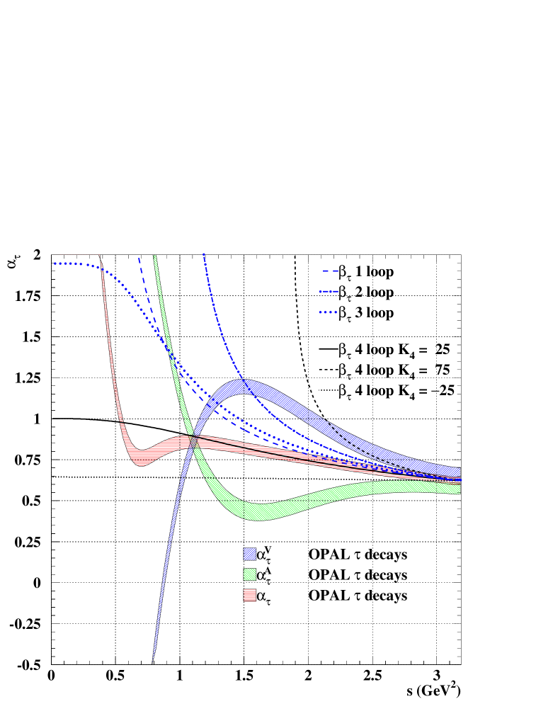
FIG. 3.: The effective charge $\alpha_{\tau}$ for non-strange hadronic decays of a hypothetical $\mathit{\tau}$ lepton with $\mathit{m_{\tau^{\prime}}^{2}=s}$ compared to solutions of the fixed order evolution equation (8) for $\alpha_{\tau}$ at two-, three-, and four-loop order. Error bands include statistical and systematic errors.

The one-loop “time-like” effective coupling [3, 4, 5]

$$\alpha_{\rm eff}(s)=\frac{4\pi}{\beta_{0}}\left\{\frac{1}{2}-\frac{1}{\pi}\arctan\left[\frac{1}{\pi}\ln\frac{s}{\Lambda^{2}}\right]\right\}$$ (9)

is obtained from the analytic continuation of the one-loop coupling $\alpha_{\rm s}(Q^{2})=(4\pi)/[\beta_{0}\ln(Q^{2}/\Lambda^{2})]$ which defines the spectral density ${\rm d}\alpha_{\rm eff}(s)/{\rm d}\ln s=[\alpha_{\rm s}(-s+i\epsilon)-\alpha_{\rm s}(-s-i\epsilon)]/(2\pi i)$ in the same way as $R_{{\rm e}^{+}{\rm e}^{-}}(s)$ is related to the Adler $D$-function. The resulting effective coupling is finite in the infrared and freezes to the value $\alpha_{\rm eff}(s)={4\pi}/{\beta_{0}}$ as $s\to 0$. It is also instructive to expand the “time-like” effective coupling for large $s$,

$$\alpha_{\rm eff}(s) = \frac{4\pi}{\beta_{0}\ln\left(s/\Lambda^{2}\right)}\left\{1-\frac{1}{3}\frac{\pi^{2}}{\ln^{2}\left(s/\Lambda^{2}\right)}+\frac{1}{5}\frac{\pi^{4}}{\ln^{4}\left(s/\Lambda^{2}\right)}+\ldots\right\}$$

$$= \alpha_{\rm s}(s)\left\{1-\frac{\pi^{2}\beta_{0}^{2}}{3}\left(\frac{\alpha_{\rm s}(s)}{4\pi}\right)^{2}+\frac{\pi^{4}\beta_{0}^{4}}{5}\left(\frac{\alpha_{\rm s}(s)}{4\pi}\right)^{4}+\ldots\right\}.$$

This shows that the “time-like” effective coupling is a resummation of $(\pi^{2}\beta_{0}^{2}\alpha_{\rm s}^{2})^{n}$-corrections to the “space-like” coupling which occurs in the analytic continuation. The “time-like” effective coupling can also be defined to higher orders (for a recent review see [50]) but the infrared behavior persists also in these cases.

The form for the finite coupling $\alpha_{\rm eff}$ given in Eq. (9) obeys standard PQCD evolution at LO. Thus one can have a solution for the perturbative running of the QCD coupling which obeys asymptotic freedom but does not have a Landau singularity.

The evolution of the modified $\tilde{\alpha}_{V}(Q^{2},\Lambda_{\rm gc}^{2})$ coupling is to leading order governed by the evolution equation,

$$\frac{{\rm d}\tilde{a}_{V}(Q^{2},\Lambda_{\rm gc}^{2})}{{\rm d}\ln Q^{2}}=-\tilde{\beta}_{0}(\Lambda_{\rm gc}/Q)\tilde{a}_{V}^{2}(Q^{2},\Lambda_{\rm gc}^{2}),$$ (10)

where

$$\tilde{\beta}_{0}(\Lambda_{\rm gc}/Q)=5-12\frac{\Lambda_{\rm gc}^{2}}{Q^{2}}+\left(12\frac{\Lambda_{\rm gc}^{3}}{Q^{3}}-6\frac{\Lambda_{\rm gc}}{Q}+\frac{3}{2}\frac{Q}{\Lambda_{\rm gc}}\right)\ln\frac{Q+2\Lambda_{\rm gc}}{Q-2\Lambda_{\rm gc}}-\frac{2}{3}n_{\rm f}.$$ (11)

The difference compared to the ordinary evolution equation is thus that the gluonic contribution to $\beta_{0}$ freezes out at a scale $Q\sim\Lambda_{\rm gc}$ – the scale of the gluon condensate.

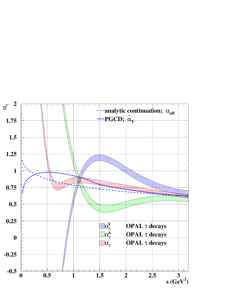
FIG. 4.: The effective charge $\alpha_{\tau}$ for non-strange hadronic decays of a hypothetical $\mathit{\tau}$ lepton with $\mathit{m_{\tau^{\prime}}^{2}=s}$ compared to the one-loop “time-like” effective coupling $\alpha_{\rm eff}(s)$ and the modified $\tilde{\alpha}_{V}$ coupling calculated from the static quark potential using perturbative gluon condensate dynamics. Error bands include statistical and systematic errors.

Fig. 4 shows a comparison of the experimentally determined effective charge $\alpha_{\tau}(s)$ with the one-loop “time-like” effective coupling $\alpha_{\rm eff}(s)$ and the modified $\tilde{\alpha}_{V}$ coupling calculated from the static quark potential using perturbative gluon condensate dynamics. In both cases the solutions have been normalized to the data at $m_{\tau}$. In addition, when solving the evolution equation for $\tilde{\alpha}_{V}$ (10) we have used the value $\Lambda_{\rm gc}=581\,{\rm MeV}$ which makes the solution to the one-loop evolution equation (8) agree with the data at $m_{\tau}$ if one sets $\Lambda=\Lambda_{\rm gc}$. As can be seen from the figure, the data on $\alpha_{\tau}(s)$ agrees well qualitatively with both of these simple examples of freezing couplings down to the scale $s\simeq 1\,{\rm GeV}^{2}$. Below this scale the non-perturbative effects in $\alpha_{\tau}(s)$ associated with the single pion pole in the axial vector current and the double pion peak in the vector current starts to dominate and makes a direct comparison with models which do not contain the spectrum of hadrons less meaningful.

IV Conclusions

The results of this paper show the advantages of defining the QCD coupling directly from a physical observable. The resulting effective coupling can be defined even at low scales, it is finite and analytic, and it has no scheme or renormalization scale ambiguities. As we have shown, the hadronic decays of the $\tau$ lepton can be used to determine the effective charge $\alpha_{\tau}(m^{2}_{\tau^{\prime}})$ for a hypothetical $\tau$-lepton with mass in the range $0<m_{\tau^{\prime}}<m_{\tau}$. The high precision of $\tau$ hadronic decay data thus provides a precise standard definition for the fundamental QCD coupling. QCD predictions for other observables can then be expressed as functions of this coupling $\alpha_{\tau}(s)$, thus relating observable to observable.

An important feature of $\alpha_{\tau}(s)$ is its apparent near constant behavior at low mass scales. The empirical results using the OPAL data are consistent with the freezing of the physical coupling at mass scales $s=m^{2}_{\tau^{\prime}}$ of order $1\,{\rm GeV}^{2}$ with a magnitude $\alpha_{\tau}\sim 0.9\pm 0.1$. These results contrast dramatically with standard expectations of a divergent coupling based on the universal two-loop coupling which becomes infinite at small mass scales. At higher orders of perturbation theory for the beta function, the behavior of the coupling is scheme dependent and in addition it is dominated by the highest order term. In the physical $\alpha_{\tau}$-scheme the behavior of the coupling in the infrared is not so clear. At 3-loops the $\alpha_{\tau}(s)$ coupling has an infrared fixed point whereas at higher orders the behavior of the coupling is not known. Estimates of the 4-loop term indicate both an infrared fixed point as well as a divergent behavior.

Recently it has been argued by Howe and Maxwell [49] that the effective charge $\alpha_{R}(s)$ has an infrared fixed point to all orders in perturbation theory. Given the commensurate scale relation between $\alpha_{\tau}$ and $\alpha_{R}$ this should then also be true for $\alpha_{\tau}(s)$. A simple example of the mechanism behind such a perturbative infrared fixed point is given by the effective “time-like” one-loop coupling $\alpha_{\rm eff}(s)$ which agrees well qualitatively with the empirically determined coupling. Another mechanism which also gives an infrared fixed point in qualitative agreement with the data is given by the perturbative gluon condensate dynamics. These simple examples show that indeed the empirical behavior $\alpha_{\tau}(s)$ is consistent with an infrared fixed point.

As we have discussed in the introduction, effective charges defined from different observables are related in perturbative QCD to each other at leading twist through commensurate scale relations [10]. The perturbative coefficients which appear in these relations are identical to those in conformal QCD; i.e. the theory defined with a zero $\beta$ function. The effects of the nonzero $\beta$ function of physical QCD are absorbed into the scale of the effective couplings. Examples are the relations between $\alpha_{R}$ and $\alpha_{\tau}$ and the generalized Crewther relation, which relates the effective charge defined from the Bjorken sum rule for $g_{1}(x,Q^{2})$ to the Adler coupling defined from ${\rm e}^{+}{\rm e}^{-}$ annihilation through a geometric series [12].

Since $\alpha_{\tau}(m^{2}_{\tau})$ has effectively constant behavior at small mass scales, the commensurate scale relations between $\alpha_{\tau}$ and other physical couplings imply that at leading twist all effective charges have a similar fixed-point behavior in the infrared regime. In particular, our results are consistent with the infrared freezing of $\alpha_{R}$ at low $s$ obtained by Mattingly and Stevenson [47].

The commensurate scale relations [10] can of course also be used at larger scales in order to compare experimental results from different observables. For example, the $\alpha_{\tau}$ effective charge can be evolved to the commensurate scale of another observable which one wants to compare with. This way the results can be compared directly, free of theoretical conventions, instead of by first extracting $\alpha_{\hbox{$\overline{\hbox{MS}}$}}(M^{2}_{Z})$ and then comparing. Beyond leading twist one can also include power-corrections in the commensurate scale relations and determine non-perturbative parameters in a standard way. Ultimately one could also envision to use a physical effective charge in the dispersive approach. As we have shown, the four-loop evolution of $\alpha_{\tau}$ with $K_{4}^{\overline{\rm MS}}=25$ gives a good description of the data down to $s\sim 1\,{\rm GeV}^{2}$ and could thus be used as an effective model for the $\alpha_{\tau}$ coupling in the low-energy regime.

The near constancy of the effective QCD coupling at small scales helps explain the empirical success of dimensional counting rules for the power law fall-off of form factors and fixed angle scaling (for a review see ref. [51]). As shown in ref. [52], one can calculate the hard scattering amplitude $T_{H}$ for such processes [53] without scale ambiguity in terms of the effective charge $\alpha_{\tau}$ or $\alpha_{R}$ using commensurate scale relations. The effective coupling is evaluated in the regime where the coupling is approximately constant, in contrast to the rapidly varying behavior from powers of $\alpha_{\rm s}$ predicted by perturbation theory (the universal two-loop coupling). For example, the nucleon form factors are proportional at leading order to two powers of $\alpha_{\rm s}$ evaluated at low scales in addition to two powers of $1/q^{2}$; The pion photoproduction amplitude at fixed angles is proportional at leading order to three powers of the QCD coupling. The essential variation from leading-twist counting-rule behavior then only arises from the anomalous dimensions of the hadron distribution amplitudes.

The large magnitude that we find $\alpha_{\tau}\sim 0.9\pm 0.1$ also implies a substantially larger normalization for the pion form factor and other exclusive observables than estimates based on a canonical value $\alpha_{\rm s}\sim 0.3$. The corresponding larger value of $\alpha^{n}_{\rm s}$ associated with the exchange of $n$ gluons in the hard scattering amplitude could eliminate much of the discrepancy between data and previous estimates of the PQCD predictions for the normalization of exclusive hard scattering amplitudes.

A The $\beta$-function in the $\overline{\rm MS}$ and $\alpha_{\tau}$ schemes

The perturbative expansion of the $\beta$ function is given by,

$$\frac{{\rm d}a_{\rm s}(s)}{{\rm d}\ln s}=-\beta_{0}a_{\rm s}^{2}(s)-\beta_{1}a_{\rm s}^{3}(s)-\beta_{2}a_{\rm s}^{4}(s)-\beta_{3}a_{\rm s}^{5}(s)-\dots,$$ (A1)

where $a_{\rm s}(s)=\alpha_{\rm s}(s)/(4\pi)$. The first two terms in the $\beta$-function [54, 55, 56, 57, 58],

$$\beta_{0} = 11-\frac{2}{3}n_{\rm f},$$

$$\beta_{1} = 102-\frac{38}{3}n_{\rm f},$$

are universal at leading twist whereas the higher order terms are scheme dependent. In the $\overline{\rm MS}$ scheme the first two scheme dependent coefficients are known [59, 60, 61]:

$$\beta_{2}^{\overline{\rm MS}} = \frac{2857}{2}-\frac{5033}{18}n_{\rm f}+\frac{325}{54}n_{\rm f}^{2},$$ (A2)

$$\beta_{3}^{\overline{\rm MS}} = \frac{149753}{6}+3564\,\zeta_{3}-\left(\frac{1078361}{162}+\frac{6508}{27}\zeta_{3}\right)n_{\rm f}$$ (A4)

$$+\left(\frac{50065}{162}+\frac{6472}{81}\zeta_{3}\right)n_{\rm f}^{2}+\frac{1093}{729}n_{\rm f}^{3}.$$

In case of the $\alpha_{\tau}$ scheme, $\beta_{\tau,2}$ is known exactly whereas for $\beta_{\tau,3}$ there are only estimates.

Since the three- and four-loop coefficients in the $\beta$-function are known in the $\overline{\rm MS}$-scheme, the corresponding coefficients (or estimates thereof) can be obtained from the perturbative expansion of $\alpha_{\tau}$ in the $\overline{\rm MS}$-scheme. Starting from the perturbative expansion of the Adler D-function for the photon vacuum polarization:

$$D(-s)=-4\pi^{2}s\frac{{\rm d}\Pi^{\gamma}(-s)}{{\rm d}s}=\sum_{f}Q_{f}^{2}\left(1+\sum_{n=1}^{4}D_{n}\frac{\alpha_{\rm s}^{n}(s)}{\pi^{n}}\right),$$ (A5)

with the known coefficients [62, 63, 64, 65, 66]

$$D_{1} = 1,$$ (A6)

$$D_{2} = \frac{365}{24}-11\,\zeta_{3}-\left(\frac{11}{12}-\frac{2}{3}\zeta_{3}\right)n_{\rm f},$$ (A7)

$$D_{3}^{\overline{\rm MS}} = \frac{87029}{288}-\frac{1103}{4}\zeta_{3}+\frac{275}{6}\zeta_{5}+\left(-\frac{7847}{216}+\frac{262}{9}\zeta_{3}-\frac{25}{9}\zeta_{5}\right)n_{\rm f}$$ (A9)

$$+\left(\frac{151}{162}-\frac{19}{27}\zeta_{3}\right)n_{\rm f}^{2}+\left(\frac{55}{72}-\frac{5}{3}\zeta_{3}\right)\frac{\displaystyle\left(\sum_{f}Q_{f}\right)^{2}}{\displaystyle N_{\rm c}\sum_{f}Q_{f}^{2}}$$

one can calculate the following expression for $\alpha_{\tau}$ where $n_{\rm f}=3$ is assumed for the $\beta_{n}$:

$$\frac{\alpha_{\tau}(s)}{\pi} = \frac{\alpha_{\hbox{$\overline{\hbox{MS}}$}}(s)}{\pi}+\left(\frac{19}{48}\beta_{0}{}+K_{2}\right)\frac{\alpha_{\hbox{$\overline{\hbox{MS}}$}}^{2}(s)}{\pi^{2}}$$ (A13)

$$+\left\{\left[\frac{265}{1152}-\frac{1}{48}\pi^{2}\right]\beta_{0}^{2}{}+\frac{19}{192}\beta_{1}{}+\frac{19}{24}\beta_{0}{}\,K_{2}+K_{3}^{\overline{\rm MS}}\right\}\frac{\alpha_{\hbox{$\overline{\hbox{MS}}$}}^{3}(s)}{\pi^{3}}$$

$$+\left\{\left[\frac{3355}{18432}-\frac{19}{768}\pi^{2}\right]\beta_{0}^{3}{}+\left[\frac{1325}{9216}-\frac{5}{384}\pi^{2}\right]\beta_{0}{}\,\beta_{1}{}+\frac{19}{768}\beta_{2}^{\overline{\rm MS}}{}\right.$$

$$\left.\quad\!\!+\left[\left(\frac{265}{384}-\frac{1}{16}\pi^{2}\right)\beta_{0}^{2}{}+\frac{19}{96}\beta_{1}{}\right]\!K_{2}+\frac{19}{16}\beta_{0}{}\,K_{3}^{\overline{\rm MS}}+K_{4}^{\overline{\rm MS}}\right\}\!\frac{\alpha_{\hbox{$\overline{\hbox{MS}}$}}^{4}(s)}{\pi^{4}},$$

where, as is customary in the $\tau$ literature, we use the following notation for the $D_{n}$ with ${\rm f}=\{\rm u,d,s\}$:

$$K_{1} = D_{1}=1,$$ (A14)

$$K_{2} = D_{2}(n_{\rm f}=3)=\frac{299}{24}-9\,\zeta_{3},$$ (A15)

$$K_{3}^{\overline{\rm MS}} = D_{3}^{\overline{\rm MS}}(n_{\rm f}=3)=\frac{58057}{288}-\frac{779}{4}\zeta_{3}+\frac{75}{2}\zeta_{5}$$ (A16)

$$K_{4}^{\overline{\rm MS}} \sim 25\pm 50,$$ (A17)

The last coefficient above is only an estimate [30] but it is often used to evaluate the uncertainty resulting from the missing higher order terms.

Finally, the resulting non-universal $\beta$-function coefficients in the $\alpha_{\tau}$-scheme are then given by:

$$\beta_{\tau,2} = \beta_{2}^{\overline{\rm MS}}{}+\left(-\frac{299}{6}+36\,\zeta_{3}\right)\beta_{1}{}+\left(\frac{169}{144}-\frac{1}{3}\pi^{2}\right)\beta_{0}^{3}{}$$ (A19)

$$+\left(\frac{26713}{36}+472\,\zeta_{3}+600\,\zeta_{5}-1296\,\zeta^{2}_{3}\right)\beta_{0}{}$$

$$= \frac{79813}{16}+6552\,\zeta_{3}+5400\,\zeta_{5}-243\,\pi^{2}-11664\,\zeta^{2}_{3}\simeq-789,$$ (A20)

$$\beta_{\tau,3} = \beta_{3}^{\overline{\rm MS}}{}+\left(-\frac{299}{3}+72\,\zeta_{3}\right)\beta_{2}^{\overline{\rm MS}}{}+\left(\frac{89401}{36}-3588\,\zeta_{3}+1296\,\zeta_{3}^{2}\right)\beta_{1}$$ (A23)

$$+\frac{1819}{432}\beta_{0}^{4}{}+\left(\frac{845}{144}-\frac{5}{3}\pi^{2}\right)\beta_{1}{}\,\beta_{0}^{2}{}+\left(-\frac{12673115}{27}+555556\,\zeta_{3}\right.$$

$$\left.\phantom{\frac{1}{2}}-179400\,\zeta_{5}+129600\,\zeta_{3}\,\zeta_{5}+101952\,\zeta_{3}^{2}-186624\,\zeta_{3}^{3}+128\,K_{4}^{\overline{\rm MS}}\right)\beta_{0}{}$$

$$= -\frac{585179735}{144}+4820288\,\zeta_{3}-1614600\,\zeta_{5}+1166400\,\zeta_{3}\,\zeta_{5}$$ (A25)

$$+1000512\,\zeta^{2}_{3}-8640\,\pi^{2}-1679616\,\zeta^{3}_{3}+1152\,K_{4}^{\overline{\rm MS}}\simeq-46776+1152\,K_{4}^{\overline{\rm MS}}.$$

Our results agree with the numerical results published in [36].

REFERENCES

- [1] M. A. Shifman, A. I. Vainshtein and V. I. Zakharov, Nucl. Phys. B147, 385 (1979).
- [2] M. Beneke, Phys. Rept. 317, 1 (1999) [arXiv:hep-ph/9807443].
- [3] M. Beneke and V. M. Braun, Phys. Lett. B348, 513 (1995) [arXiv:hep-ph/9411229].
- [4] P. Ball, M. Beneke and V. M. Braun, Nucl. Phys. B452, 563 (1995) [arXiv:hep-ph/9502300].
- [5] Y. L. Dokshitzer, G. Marchesini and B. R. Webber, Nucl. Phys. B469, 93 (1996) [arXiv:hep-ph/9512336].
- [6] G. Grunberg, Phys. Lett. B95, 70 (1980) [Erratum-ibid. B110, 501 (1982)].
- [7] G. Grunberg, Phys. Rev. D29, 2315 (1984).
- [8] S. J. Brodsky, M. S. Gill, M. Melles and J. Rathsman, Phys. Rev. D58, 116006 (1998) [arXiv:hep-ph/9801330].
- [9] S. J. Brodsky, M. Melles and J. Rathsman, Phys. Rev. D60, 096006 (1999) [arXiv:hep-ph/9906324].
- [10] S. J. Brodsky and H. J. Lu, Phys. Rev. D51, 3652 (1995) [arXiv:hep-ph/9405218].
- [11] D. J. Broadhurst and A. L. Kataev, Phys. Lett. B315, 179 (1993) [arXiv:hep-ph/9308274].
- [12] S. J. Brodsky, G. T. Gabadadze, A. L. Kataev and H. J. Lu, Phys. Lett. B372, 133 (1996) [arXiv:hep-ph/9512367].
- [13] S. J. Brodsky, E. Gardi, G. Grunberg and J. Rathsman, Phys. Rev. D63, 094017 (2001) [arXiv:hep-ph/0002065].
- [14] J. Rathsman, in Proc. of the 5th International Symposium on Radiative Corrections (RADCOR 2000) ed. Howard E. Haber, arXiv:hep-ph/0101248.
- [15] E. Gardi and G. Grunberg, Phys. Lett. B517, 215 (2001) [arXiv:hep-ph/0107300].
- [16] J.D. Bjorken and S.D. Drell, Relativistic Quantum Fields, McGraw-Hill, New-York, 1965.
- [17] S. J. Brodsky, G. P. Lepage and P. B. Mackenzie, Phys. Rev. D28, 228 (1983).
- [18] K. Hornbostel, G. P. Lepage and C. Morningstar, hep-ph/0208224 (2002).
- [19] S. J. Brodsky and P. Huet, Phys. Lett. B417, 145 (1998) [arXiv:hep-ph/9707543].
- [20] L. Susskind, in Les Houches 1976, Proceedings, Weak and Electromagnetic Interactions At High Energies, 207-308, Amsterdam 1977.
- [21] T. Appelquist, M. Dine and I. J. Muzinich, Phys. Rev. D17, 2074 (1978).
- [22] J. M. Cornwall, Phys. Rev. D26, 1453 (1982).
- [23] J. M. Cornwall and J. Papavassiliou, Phys. Rev. D40, 3474 (1989).
- [24] N. J. Watson, Nucl. Phys. B494, 388 (1997) [arXiv:hep-ph/9606381].
- [25] D. Binosi and J. Papavassiliou, hep-ph/0209016 (2002).
- [26] E. Braaten, Phys. Rev. Lett. 60, 1606 (1988).
- [27] E. Braaten, Phys. Rev. D39, 1458 (1989).
- [28] S. Narison and A. Pich, Phys. Lett. B211, 183 (1988).
- [29] E. Braaten, S. Narison and A. Pich, Nucl. Phys. B373, 581 (1992).
- [30] F. Le Diberder and A. Pich, Phys. Lett. B289, 165 (1992).
- [31] M. Neubert, Nucl. Phys. B463, 511 (1996) [arXiv:hep-ph/9509432].
- [32] C. J. Maxwell and D. G. Tonge, Nucl. Phys. B481, 681 (1996) [arXiv:hep-ph/9606392].
- [33] M. Girone and M. Neubert, Phys. Rev. Lett. 76, 3061 (1996) [arXiv:hep-ph/9511392].
- [34] (ALEPH Collaboration), R. Barate et al., Eur. Phys. J. C4, 409 (1998).
- [35] (OPAL Collaboration), K. Ackerstaff et al., Eur. Phys. J. C7, 571 (1999)
- [36] J. G. Körner, F. Krajewski and A. A. Pivovarov, Phys. Rev. D63, 036001 (2001) [arXiv:hep-ph/0002166].
- [37] K. A. Milton, I. L. Solovtsov, O. P. Solovtsova and V. I. Yasnov, Eur. Phys. J. C14, 495 (2000) [arXiv:hep-ph/0003030].
- [38] G. Cvetic and T. Lee, Phys. Rev. D64, 014030 (2001) [arXiv:hep-ph/0101297].
- [39] G. Cvetic, C. Dib, T. Lee and I. Schmidt, Phys. Rev. D64, 093016 (2001) [arXiv:hep-ph/0106024].
- [40] W. J. Marciano and A. Sirlin, Phys. Rev. Lett. 61, 1815 (1988).
- [41] (Particle Data Group Collaboration), R. M. Barnett et al., Phys. Rev. D54, 1 (1996).
- [42] S. J. Brodsky, J. R. Peláez and N. Toumbas, Phys. Rev. D60, 037501 (1999) [arXiv:hep-ph/9810424].
- [43] S. Menke, Nucl. Phys. (Proc. Suppl.) B76, 299 (1999), and B86, 196 (2000).
- [44] B. L. Ioffe and K. N. Zyablyuk, Nucl. Phys. A687, 437 (2001) [arXiv:hep-ph/0010089].
- [45] B. V. Geshkenbein, B. L. Ioffe and K. N. Zyablyuk, Phys. Rev. D64, 093009 (2001) [arXiv:hep-ph/0104048].
- [46] (Particle Data Group Collaboration), K. Hagiwara et al., Phys. Rev. D66, 010001 (2002).
- [47] A. C. Mattingly and P. M. Stevenson, Phys. Rev. D49, 437 (1994) [arXiv:hep-ph/9307266].
- [48] P. Hoyer and J. Rathsman, JHEP 0105, 020 (2001) [arXiv:hep-ph/0011209].
- [49] D. M. Howe and C. J. Maxwell, Phys. Lett. B541, 129 (2002) [arXiv:hep-ph/0204036].
- [50] D. V. Shirkov, Eur. Phys. J. C22, 331 (2001) [arXiv:hep-ph/0107282].
- [51] S. J. Brodsky and G. P. Lepage, SLAC-PUB-4947 (1989).
- [52] S. J. Brodsky, C. R. Ji, A. Pang and D. G. Robertson, Phys. Rev. D57, 245 (1998) [arXiv:hep-ph/9705221].
- [53] G. P. Lepage and S. J. Brodsky, Phys. Rev. D22, 2157 (1980).
- [54] D. J. Gross and F. Wilczek, Phys. Rev. Lett. 30, 1343 (1973).
- [55] H. D. Politzer, Phys. Rev. Lett. 30, 1346 (1973).
- [56] W.E. Caswell, Phys. Rev. Lett. 33, 244 (1974).
- [57] D. R. Jones, Nucl. Phys. B75, 531 (1974).
- [58] E. Egorian and O. V. Tarasov, Theor. Math. Phys. 41, 863 (1979) [Teor. Mat. Fiz. 41, 26 (1979)].
- [59] O. V. Tarasov, A. A. Vladimirov and A. Y. Zharkov, Phys. Lett. B93, 429 (1980).
- [60] S. A. Larin and J. A. Vermaseren, Phys. Lett. B303, 334 (1993) [arXiv:hep-ph/9302208].
- [61] T. van Ritbergen, J. A. Vermaseren and S. A. Larin, Phys. Lett. B400, 379 (1997) [arXiv:hep-ph/9701390].
- [62] K. G. Chetyrkin, A. L. Kataev and F. V. Tkachov, Phys. Lett. B85, 277 (1979).
- [63] M. Dine and J. R. Sapirstein, Phys. Rev. Lett. 43, 668 (1979).
- [64] W. Celmaster and R. J. Gonsalves, Phys. Rev. Lett. 44, 560 (1980).
- [65] S. G. Gorishnii, A. L. Kataev and S. A. Larin, Phys. Lett. B259, 144 (1991).
- [66] L. R. Surguladze and M. A. Samuel, Phys. Rev. Lett. 66, 560 (1991) [Erratum-ibid. 66, 2416 (1991)].