Abstract

We introduce a new parameterisation of the effect of unknown corrections from new physics on quark and lepton mass matrices. This parameterisation is used in order to study how the hierarchies of quark masses and mixing angles are modified by random perturbations of the Yukawa matrices. We discuss several examples of flavour relations predicted by different textures, analysing how these relations are influenced by the random perturbations. We also comment on the unlikely possibility that unknown corrections contribute significantly to the hierarchy of masses and mixings.

1 Introduction

The observed quark masses and Cabibbo-Kobayashi-Maskawa (CKM) mixing angles show a hierarchy $m_{t}\gg m_{c}\gg m_{u}$, $m_{b}\gg m_{s}\gg m_{d}$, $|V_{us}|\gg|V_{cb}|\gg|V_{ub}|$ that points to an underlying structure in the Yukawa couplings of up and down-type quarks to the Higgs boson. This fact has motivated the introduction of several models of mass matrices trying to reproduce the experimental values of the quark masses and CKM matrix elements using well-structured Yukawa patterns. In general, these models consider that at very high energies, and for some reason unknown at present, a weak basis is privileged among the infinite set of equivalent weak bases related by rotations of the quark fields in flavour space. In this privileged basis, some flavour symmetry reduces the number of free parameters in the Yukawa matrices, leading to relations among masses and mixing angles that can be experimentally tested. Examples of these models include patterns with texture zeros [1], democratic Yukawa couplings [2] or other symmetries (see for instance [3, 4]).

At lower scales, where the underlying flavour symmetry is broken, the Yukawa textures are modified by renormalisation group (RG) evolution and other radiative corrections, with several contributions from Standard Model (SM) and new physics. These corrections are unknown, and constitute what is called “anarchy”. The “anarchy” may in principle lead to modifications in the predictions of the original patterns. The stability of these predictions, when the new contributions are included, can be estimated with the addition of random perturbations to the Yukawa matrices in the Lagrangian. Of course, the new physics contributions are not random in nature, and could be computed if the complete theory was known. At any rate, a simulation with random perturbations shows which quantities are stable and which are not, and to what extent they are modified in this case. It is already known that the strong hierarchy of masses and mixings is not likely to be originated from “anarchy” [5]. Recently, it has been argued [6] that in the quark sector the possible contributions of the latter must be very small, in order to preserve a hierarchical structure. However, this result has been obtained for a particular texture of Yukawa couplings and in a particular weak basis. It would be desirable to obtain a basis and model-independent result indicating, at least qualitatively, how the “anarchy” could change the hierarchy of quark masses and mixings.

In the lepton sector the situation is rather different. The masses of the charged leptons have been precisely measured, but the knowledge about neutrino masses and mixings is still rather poor. After the measurement of atmospheric neutrino oscillations, with $\sin^{2}\!\theta_{\mathrm{atm}}\geq 0.92$, $\Delta m^{2}_{\mathrm{atm}}=(1.6-3.9)\times 10^{-3}$ GeV [7], it is clear that the pattern of lepton masses and mixings is completely different from the one in the quark sector. In this direction, it has been suggested that the neutrino mass matrices might be generated just from “anarchy” [8] (see also Ref. [9]). A complete analysis is not yet possible in the lepton sector, for several reasons: (i) some of the mixing angles have not still been measured; (ii) the neutrino masses remain unknown and only the differences of squared masses can be extracted from oscillation data; (iii) the Dirac or Majorana nature of the neutrinos is yet to be determined, and in the first case Majorana-type mass terms are not present.

Our aim here is to study how the “anarchy” would affect a hierarchical pattern, as the one found in the quark sector. We first derive the formal structure of the unknown corrections to the mass matrices, both for the case of quarks and leptons. We use this formalism to investigate how random perturbations modify a given hierarchy of quark masses and mixings. Then we discuss the effect in some relations involving masses and CKM matrix elements, which are predicted in several models of Yukawa patterns existing in the literature. Finally, we explore the possibility of a significative enhancement of the hierarchy of quark masses due to the “anarchy”.

2 Anarchy in the mass matrices

The starting point of our argument will be the observation that physical quantities cannot depend on the weak basis chosen for the quark fields. In the SM, the mass terms of the Lagrangian are written as

$$\mathcal{L}_{m}=-\bar{u}_{L}v\,Y^{u}u_{R}-\bar{d}_{L}v\,Y^{d}d_{R}+\mathrm{h.c.}\,,$$ (1)

with $v=174$ GeV the vacuum expectation value (VEV) of the Higgs boson, and $Y^{u}$, $Y^{d}$ the Yukawa matrices, of dimension $3\times 3$ in flavour space. In some SM extensions, for instance in the minimal supersymmetric Standard Model (MSSM), the masses are originated from the VEV’s of two Higgs bosons, $v_{u}$ and $v_{d}$, with $v_{u}^{2}+v_{d}^{2}=v^{2}$. Defining $\beta$ by $\tan\beta=v_{u}/v_{d}$, the mass matrices for up and down quarks are in this case $v\sin\beta\,Y^{u}$ and $v\cos\beta\,Y^{d}$, respectively, with an extra $\beta$-dependent factor. We later comment on how this possibility modifies our analysis.

It is well known that under a change of basis

$$\left(\!\begin{array}[]{c}u_{L}\\ d_{L}\end{array}\!\right)=U_{L}\left(\!\begin{array}[]{c}u^{\prime}_{L}\\ d^{\prime}_{L}\end{array}\!\right)~{}~{},~{}~{}~{}u_{R}=U_{R}^{u}~{}u^{\prime}_{R}~{}~{},~{}~{}~{}d_{R}=U_{R}^{d}~{}d^{\prime}_{R}$$ (2)

the Yukawa matrices transform as

$$Y^{u}\to U_{L}^{\dagger}\,Y^{u}\,U_{R}^{u}~{}~{},~{}~{}~{}Y^{d}\to U_{L}^{\dagger}\,Y^{d}\,U_{R}^{d}\,.$$ (3)

Let us assume that some perturbations are added to the original Yukawa matrices,

$$Y^{u}\to Y^{u}+\delta Y^{u}~{}~{},~{}~{}~{}Y^{d}\to Y^{d}+\delta Y^{d}\,.$$ (4)

The matrices $\delta Y^{u}$, $\delta Y^{d}$ are functions of $Y^{u}$, $Y^{d}$ and other SM and new physics parameters. Under the change of basis in Eqs. (3), the perturbations must transform as

$$\delta Y^{u}\to U_{L}^{\dagger}\,\delta Y^{u}\,U_{R}^{u}~{}~{},~{}~{}~{}\delta Y^{d}\to U_{L}^{\dagger}\,\delta Y^{d}\,U_{R}^{d}\,,$$ (5)

since the physical observables must be independent of the choice of weak basis . These transformation laws imply that the perturbations have the form

$$\delta Y^{u} = \lambda_{u}\,Y^{u}+\zeta_{u}\,Y^{u}Y^{u\dagger}Y^{u}+\eta_{u}\,Y^{d}Y^{d\dagger}Y^{u}+\cdots\,,$$

$$\delta Y^{d} = \lambda_{d}\,Y^{d}+\zeta_{d}\,Y^{d}Y^{d\dagger}Y^{d}+\eta_{d}\,Y^{u}Y^{u\dagger}Y^{d}+\cdots\,.$$ (6)

The dimensionless coefficients $\lambda_{i}$, $\zeta_{i}$, $\eta_{i}$ may be functions of $Y^{u}$ and $Y^{d}$ that are invariant under $\mathrm{SU}(3)$ flavour rotations, e.g. $\mathrm{tr}\;Y^{u}Y^{u\dagger}$, $\mathrm{tr}\;Y^{d}Y^{d\dagger}$, etc. and of other SM and new physics parameters as well. The higher-order terms are expected to be smaller (if perturbation theory is valid), thus in the expansions of Eqs. (6) the products with five or more Yukawa matrices have been omitted. The effect of the $\lambda_{i}$ terms in Eqs. (6) is to rescale the masses by common factors $(1+\lambda_{u})$ for up quarks and $(1+\lambda_{d})$ for down quarks, without affecting the hierarchy and the mixing. The $\zeta_{i}$ terms also rescale the masses, but with different factors for each quark, $m_{q}\to m_{q}\,(1+\zeta_{i}\,m_{q}^{2}/v^{2})$, and then they modify the hierarchies. The $\eta_{i}$ terms are the lowest-order ones that modify the CKM matrix.

In principle, in SM extensions there may exist a matrix $X$ (not necessarily square) of couplings between the quarks and other particles, either transforming on the left or on the right side as one of the Yukawa matrices. For instance, if $X$ transforms under the change of basis in Eqs. (3) as

$$X\to U_{L}^{\dagger}\,X\,U_{R}^{X}\,,$$ (7)

this matrix would originate terms $XX^{\dagger}Y^{u}$ and $XX^{\dagger}Y^{d}$ in Eqs. (6). However, if diagrams involving $X$ couplings gave significant corrections to the Higgs Yukawa vertices with a new flavour structure, analogous diagrams with a photon, gluon or $Z$ boson would give similar contributions to flavour-changing processes, which are experimentally very suppressed. Thus we disregard this possibility in the following.

It is worthwhile noting that the formal structure of the perturbations to the Yukawa matrices, derived here from weak-basis independence arguments, coincides with the expression of the RG equations in the SM. Setting for instance in Eqs. (6)

$$\lambda_{u} = \frac{1}{16\pi^{2}}\left\{\mathrm{tr}\left[3Y^{u}Y^{u\dagger}+3Y^{d}Y^{d\dagger}+Y^{e}Y^{e\dagger}\right]-\left(\frac{17}{20}g_{1}^{2}+\frac{9}{4}g_{2}^{2}+8g_{3}^{2}\right)\right\}\delta t\,,$$

$$\lambda_{d} = \frac{1}{16\pi^{2}}\left\{\mathrm{tr}\left[3Y^{u}Y^{u\dagger}+3Y^{d}Y^{d\dagger}+Y^{e}Y^{e\dagger}\right]-\left(\frac{1}{4}g_{1}^{2}+\frac{9}{4}g_{2}^{2}+8g_{3}^{2}\right)\right\}\delta t\,,$$

$$\zeta_{u} = \frac{1}{16\pi^{2}}\left\{\frac{3}{2}\right\}\delta t\,,$$

$$\zeta_{d} = \frac{1}{16\pi^{2}}\left\{\frac{3}{2}\right\}\delta t\,,$$

$$\eta_{u} = \frac{1}{16\pi^{2}}\left\{-\frac{3}{2}\right\}\delta t\,,$$

$$\eta_{d} = \frac{1}{16\pi^{2}}\left\{-\frac{3}{2}\right\}\delta t\,,$$ (8)

the SM one-loop RG equations for the Yukawa couplings are recovered [10, 11] . In Eqs. (8), $Y^{e}$ is the Yukawa matrix for the charged leptons, $g_{3}$, $g_{2}$ and $g_{1}$ are the coupling constants of the gauge group $\mathrm{SU}(3)\otimes\mathrm{SU}(2)\otimes\mathrm{U}(1)$ and $t=\log\mu$ the logarithm of the renormalisation scale.

In the lepton sector the analysis is more involved, because of the possible presence of Majorana fermions. In this case the mass terms of the Lagrangian read

$$\mathcal{L}_{m}=-\bar{e}_{L}v\,Y^{e}e_{R}-\frac{1}{2}\left(\bar{\nu}_{L}~{}\overline{\nu_{R}^{c}}\right)\left(\begin{array}[]{cc}M_{L}&v\,Y^{\nu}\\ v\,Y^{\nu T}&M_{R}\end{array}\right)\left(\begin{array}[]{c}\nu_{L}^{c}\\ \nu_{R}\end{array}\right)\,.$$ (9)

The Dirac mass matrices $v\,Y^{e}$ and $v\,Y^{\nu}$ arise from Yukawa couplings to the Higgs boson. The Majorana mass matrix $M_{R}$ can be included as a bare term in the Lagrangian, because the right-handed neutrinos are singlets under the gauge group. The Majorana mass term $M_{L}$ involving the left-handed neutrino fields can only exist at tree-level in a renormalisable Lagrangian if a Higgs triplet is present (this is practically excluded by precision electroweak data), and $M_{L}$ is usually set to zero. Both $M_{L}$ and $M_{R}$ are symmetric matrices. We define $M_{L}\equiv\Lambda_{L}\hat{M}_{L}$, $M_{R}\equiv\Lambda_{R}\hat{M}_{R}$, with $\Lambda_{L}$ and $\Lambda_{R}$ constants with the dimension of mass, in order to express $M_{L}$ and $M_{R}$ in terms of dimensionless matrices.

Under a change of weak basis

$$\left(\!\begin{array}[]{c}\nu_{L}\\ e_{L}\end{array}\!\right)=V_{L}\left(\!\begin{array}[]{c}\nu^{\prime}_{L}\\ e^{\prime}_{L}\end{array}\!\right)~{}~{},~{}~{}~{}\nu_{R}=V_{R}^{\nu}~{}\nu^{\prime}_{R}~{}~{},~{}~{}~{}e_{R}=V_{R}^{e}~{}e^{\prime}_{R}$$ (10)

we have

$$Y^{e} \to V_{L}^{\dagger}\,Y^{e}\,V_{R}^{e}~{}~{},~{}~{}~{}Y^{\nu}\to V_{L}^{\dagger}\,Y^{\nu}\,V_{R}^{\nu}\,,$$

$$\hat{M}_{L} \to V_{L}^{\dagger}\hat{M}_{L}V_{L}^{*}~{}~{},~{}~{}~{}\hat{M}_{R}\to V_{R}^{\nu T}\hat{M}_{R}V_{R}^{\nu}\,.$$ (11)

The computation of all the products up to order three transforming as $Y^{e}$, $Y^{\nu}$, $\hat{M}_{L}$ and $\hat{M}_{R}$ can be easily done with the programs in Ref. [12]. It is found that the perturbations to these matrices can be expanded as

$$\delta Y^{e} = \lambda_{e}\,Y^{e}+\zeta_{e}\,Y^{e}Y^{e\dagger}Y^{e}+\eta_{e1}\,Y^{\nu}Y^{\nu\dagger}Y^{e}+\eta_{e2}\,\hat{M}_{L}\hat{M}_{L}^{\dagger}Y^{e}+\cdots\,,$$

$$\delta Y^{\nu} = \lambda_{\nu}\,Y^{\nu}+\zeta_{\nu}Y^{\nu}Y^{\nu\dagger}Y^{\nu}+\eta_{\nu 1}\,Y^{e}Y^{e\dagger}Y^{\nu}+\eta_{\nu 2}\,\hat{M}_{L}\hat{M}_{L}^{\dagger}Y^{\nu}$$

$$+\xi_{\nu 1}\,Y^{\nu}\hat{M}_{R}^{\dagger}\hat{M}_{R}+\xi_{\nu 2}\,\hat{M}_{L}Y^{\nu*}\hat{M}_{R}+\cdots\,,$$

$$\delta\hat{M}_{L} = \lambda_{L}\,\hat{M}_{L}+\zeta_{L}\,\hat{M}_{L}\hat{M}_{L}^{\dagger}\hat{M}_{L}+\eta_{L1}\left(Y^{e}Y^{e\dagger}\hat{M}_{L}+\hat{M}_{L}Y^{e*}Y^{eT}\right)$$

$$+\eta_{L2}\left(Y^{\nu}Y^{\nu\dagger}\hat{M}_{L}+\hat{M}_{L}Y^{\nu*}Y^{\nu T}\right)+\chi_{L}\,Y^{\nu}\hat{M}_{R}^{\dagger}Y^{\nu T}+\cdots\,,$$

$$\delta\hat{M}_{R} = \lambda_{R}\,\hat{M}_{R}+\zeta_{R}\,\hat{M}_{R}\hat{M}_{R}^{\dagger}\hat{M}_{R}+\eta_{R}\left(M_{R}Y^{\nu\dagger}Y^{\nu}+Y^{\nu T}Y^{\nu*}M_{R}\right)$$ (12)

$$+\chi_{R}\,Y^{\nu T}\hat{M}_{L}^{\dagger}Y^{\nu}+\cdots\,,$$

where the $\lambda$, $\zeta$, $\eta$, $\xi$, $\chi$ coefficients are functions of $Y^{e}$, $Y^{\nu}$, $\hat{M}_{L}$, $\hat{M}_{R}$ and of the coupling constants, invariant under the transformations of Eqs. (11). Under additional assumptions, the number of terms can be reduced. For instance, assuming that $\hat{M}_{L}=0$ at tree-level, the terms with $\eta_{e2}$, $\eta_{\nu 2}$, $\xi_{\nu 2}$, $\lambda_{L}$, $\zeta_{L}$, $\eta_{L1}$, $\eta_{L2}$ and $\chi_{R}$ can be dropped from the expressions. Notice that even setting $\hat{M}_{L}=0$ in the Lagrangian, our argument allows a non-vanishing $\delta\hat{M}_{L}=\chi_{L}Y^{\nu}\hat{M}_{R}^{\dagger}Y^{\nu T}$ to be generated, though some symmetry in the Lagrangian may imply $\chi_{L}=0$. The analysis of the effects of the “anarchy” in the lepton sector will be presented elsewhere [13].

3 Effects of anarchy in the hierarchy of masses and mixing angles

We first study how the “anarchy” may change a hierarchical structure in the Yukawa couplings. For our discussion we take as benchmark the SM Yukawa matrices in the $\overline{\mathrm{MS}}$ scheme at the scale $M_{Z}$ (since the expressions in Eqs. (6) are basis-independent, we can use any basis for the evaluations). The values used for the quark masses are collected in Table 1. For the CKM matrix we use, in the standard parameterisation [14], $|V_{us}|=0.2224$, $|V_{ub}|=0.00362$, $|V_{cb}|=0.0402$ and $\delta=1.014$.

$m_{u}$	$0.0016$
$m_{c}$	$0.68$
$m_{t}$	$175.6$
$m_{d}$	$0.0033$
$m_{s}$	$0.067$
$m_{b}$	$2.9$

Table 1: Quark masses (in GeV) used in the numerical evaluations.

We use the perturbations to the Yukawa matrices given in Eqs. (6), with random coefficients $\lambda_{i}$, $\zeta_{i}$, $\eta_{i}$. The moduli of these six independent parameters are generated with a Gaussian distribution centred at zero, and for simplicity we assume that the standard deviations coincide:

$$\langle|\lambda_{i}|^{2}\rangle^{\frac{1}{2}}=\langle|\zeta_{i}|^{2}\rangle^{\frac{1}{2}}=\langle|\eta_{i}|^{2}\rangle^{\frac{1}{2}}\equiv\kappa\,.$$ (13)

This is not a serious bias in the analysis, because the moduli of the random parameters are not fixed to be all equal, and only the standard deviations of the distributions are assumed to be the same. The phases are generated uniformly between $0$ and $2\pi$. The only effect of the $\lambda_{i}$ terms is to change the ratio $m_{b}/m_{t}$; the mixing angles and the ratios of masses of quarks of the same charge are not modified by them. Here it is worth remarking that the situation when two different scalars give masses to the up and down-type quarks can be reproduced with the substitutions

$$Y^{u}\to Y^{u}\sin\beta~{},~{}~{}~{}Y^{d}\to Y^{d}\cos\beta$$ (14)

in Eqs. (6). This is equivalent to considering

$$\langle|\lambda_{i}|^{2}\rangle^{\frac{1}{2}} = \kappa\,,$$

$$\langle|\zeta_{u}|^{2}\rangle^{\frac{1}{2}}=\langle|\eta_{d}|^{2}\rangle^{\frac{1}{2}} = \kappa\sin^{2}\!\beta\,,$$

$$\langle|\zeta_{d}|^{2}\rangle^{\frac{1}{2}}=\langle|\eta_{u}|^{2}\rangle^{\frac{1}{2}} = \kappa\cos^{2}\!\beta$$ (15)

instead of Eqs. (13). The effect of $\tan\beta$ is to modify the standard deviations of the distributions of the random parameters. The qualitative behaviour with two scalars is the same as in the case discussed below, with only one Higgs. The quantitative behaviour is similar, as long as $\tan\beta\sim 1$.

In the study of the consequences of “anarchy” the following procedure is applied: we fix a value of $\kappa$ and generate a set of random matrices, with a number of elements between 2000 (for $\kappa\simeq 0$) and 8000 (for $\kappa\simeq 1$). We then select some quantity, for instance the ratio $m_{c}/m_{t}$, and examine its distribution over the set. The $1\sigma$ limits on this quantity are defined as the boundaries of the 68.7% confidence level central interval, evaluated from the sample of random matrices. We begin the discussion with this example of $m_{c}/m_{t}$. We find that this quantity remains fairly stable, even for relatively large values of $\kappa$, e.g. $\kappa=1$. In Fig. 1 (left) we plot the $1\sigma$ limits on $m_{c}/m_{t}$, for $\kappa$ between 0 and 1. In Fig. 1 (right) we plot the distribution of the values of $m_{c}/m_{t}$ for $\kappa=1$.

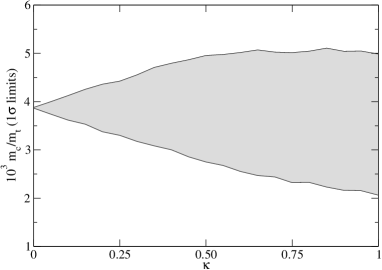
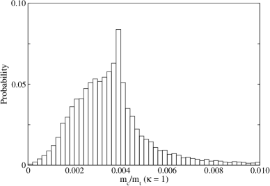
Figure 1: Effect of the random perturbations on the ratio $m_{c}/m_{t}$.

Several comments are in order:

1. The distribution of $m_{c}/m_{t}$ is peaked around the unperturbed value $(m_{c}/m_{t})_{0}=3.9\times 10^{-3}$, because the random parameters are generated with a Gaussian distribution centred at zero. It spreads over values larger and smaller than $(m_{c}/m_{t})_{0}$, but with larger $\kappa$ the smaller values are favoured. This can be observed in both plots, and evidences an average increase of $m_{t}$ with respect to $m_{c}$, due to the larger Yukawa coupling of the former. The ratio $m_{c}/m_{t}$ is modified mainly by the $\zeta_{u}$ term, giving corrections $\delta m_{c}=\zeta_{u}\,m_{c}^{3}/v^{2}$, $\delta m_{t}=\zeta_{u}\,m_{t}^{3}/v^{2}$ that are much larger for the top quark.

2. The spread of the values of $m_{c}/m_{t}$ increases with $\kappa$, as it can be expected. The growth is linear for small $\kappa$ but it is attenuated for $\kappa\geq 0.5$, as can be observed in Fig. 1 (left). The upper limit on $m_{c}/m_{t}$ reaches a “saturation” value for $\kappa\geq 0.5$ and does not increase beyond this value. This can be understood as follows: As the corrections are larger for the top quark, the ratio $m_{c}/m_{t}$ will generically be smaller, and the only chance to have a larger $m_{c}/m_{t}$ is with a cancellation between $m_{t}$ and $\delta m_{t}$. For $\kappa$ sufficiently large, the probability of this fine tuning to happen is practically constant.

3. Most of the values of $m_{c}/m_{t}$ remain close to their original value. Even for $\kappa=1$, 68.7% of the distribution is between the values $2.0\times 10^{-3}$ and $5.0\times 10^{-3}$, very similar to $(m_{c}/m_{t})_{0}$. It is noticeable the long tail of the distribution in Fig. 1 (right). For $\kappa=1$, the largest value of $m_{c}/m_{t}$ found in the set is $0.15$, for which the mass hierarchy is washed away. Such values are reached only in an extremely small fraction of the sample.

These plots must not be interpreted as providing any limit on the size of the “anarchy”, on the basis of the experimental value of $m_{c}/m_{t}$. Instead, their meaning is that the ratio $m_{c}/m_{t}$ is very stable under perturbations and the mass hierarchy is maintained (due to points 2 and 3 above): from an original value $(m_{c}/m_{t})_{0}=3.9\times 10^{-3}$ and with $\kappa=1$ we obtain ratios between $2.0\times 10^{-3}$ and $5.0\times 10^{-3}$ most of the time.

The effect of the random perturbations in the ratio $m_{s}/m_{b}$ is practically the same, as can be observed in Fig. 2. Although with different numerical values, this ratio shows the same behaviour under random perturbations as $m_{c}/m_{t}$, and the above comments apply in this case as well. The leading correction to $m_{s}/m_{b}$ is due to the $\eta_{d}$ term, $\delta m_{s}\simeq\eta_{d}\,m_{s}m_{c}^{2}/v^{2}$, $\delta m_{b}\simeq\eta_{d}\,m_{b}m_{t}^{2}/v^{2}$, and the effects are analogous.

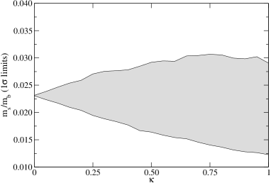
Figure 2: Effect of the random perturbations on the ratio $m_{s}/m_{b}$.

The analysis of the two mass ratios $m_{u}/m_{c}$ and $m_{d}/m_{s}$ shows that they do not change when random perturbations are added to the Yukawa matrices, remaining at the values $(m_{u}/m_{c})_{0}=2.3\times 10^{-3}$, $(m_{d}/m_{s})_{0}=0.049$. This is the same behaviour as under RG evolution [15], where it is found that these ratios depend weakly on the scale. Here we find examples where $m_{d}/m_{s}$ raises to 0.10, but this only happens in a negligibly small fraction of the sample. Therefore, the mass hierarchy between the first and second quark generations is also maintained. The remaining independent ratio $m_{b}/m_{t}$ exhibits a different behaviour, as can be readily noticed in Fig. 3. The maximum of the distribution is displaced to smaller values of $m_{b}/m_{t}$, and additionally there is a long tail for larger values of this quantity. This can be understood as follows: Setting $|V_{tb}|=1$, Eqs. (6) imply for the third generation

$$\delta m_{t} = \lambda_{u}\,m_{t}+\zeta_{u}\,m_{t}^{3}/v^{2}+\eta_{u}\,m_{t}m_{b}^{2}/v^{2}\,,$$

$$\delta m_{b} = \lambda_{d}\,m_{b}+\zeta_{d}\,m_{b}^{3}/v^{2}+\eta_{d}\,m_{b}m_{t}^{2}/v^{2}\,.$$ (16)

The enhancement for small values of $m_{b}/m_{t}$ is due to the large term $\zeta_{u}\,m_{t}^{3}/v^{2}$, while the long tail is a consequence of the term $\eta_{d}\,m_{b}m_{t}^{2}/v^{2}$, also important. The change of this ratio with respect to its original value is limited, though more pronounced than in the previous cases.

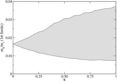
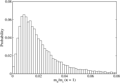
Figure 3: Effect of the random perturbations on the ratio $m_{b}/m_{t}$.

The modulus of the CKM matrix element $V_{us}$ is not affected by the random perturbations. As happens for the ratios $m_{u}/m_{c}$ and $m_{d}/m_{s}$, there are fine-tuned values of the random parameters for which the corrections yield a much larger value, for instance $|V_{us}|\sim 0.4$. We stress that this only happens in an insignificant fraction of the sample, and for the rest we find $|V_{us}|$ almost fixed at its original value. The CKM phase $\delta$ does not change either. The moduli of $V_{cb}$ and $V_{ub}$ change when the perturbations are added, but their ratio remains constant. (Besides, this is the same behaviour with RG evolution that is found for $V_{us}$, $V_{cb}$, $V_{ub}$ and the phase $\delta$ [15].) The distribution of values of $|V_{cb}|$ can be seen in Fig. 4, and coincides with the distribution of $|V_{ub}|$ up to an overall factor.

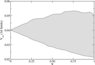
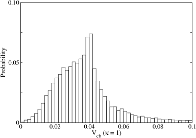
Figure 4: Effect of the random perturbations on $|V_{cb}|$.

Comparing these plots with Figs. 1 and 2 we observe that the effect of the “anarchy” on the moduli of the mixing angles $V_{cb}$ and $V_{ub}$ and in the ratios of masses $m_{c}/m_{t}$, $m_{s}/m_{b}$, $m_{u}/m_{t}$ and $m_{d}/m_{b}$ is similar. This fact is due to the formal structure of the random perturbations, and has non-trivial implications in some flavour relations in the next Section.

4 Effects in flavour relations

We have selected nine simple flavour relations predicted by several models in the literature. Here we do not pretend to test whether these relations are actually fulfilled by experimental data. Such analysis ought to be carried out at a very high energy scale, of the order of the unification scale $M_{X}\sim 10^{16}$ GeV (where a hypothetical flavour symmetry is unbroken), using the Yukawa matrices at that scale. Instead, our aim is to investigate whether these relations are modified by the “anarchy”. This analysis can be safely done at the scale $M_{Z}$. We prefer to perform the simulations at this scale because the extrapolation to the unification scale $M_{X}$ depends on the particle content of the theory between $M_{Z}$ and $M_{X}$, and therefore it is different in the SM and its extensions. For instance, in the MSSM the running of some parameters, like $|V_{ub}|$, depends strongly on the parameter $\tan\beta$.

Relation I is [16, 17]

$$|V_{us}|=\sqrt{\frac{m_{d}}{m_{s}}}\,,$$ (17)

predicted for instance by the five textures proposed in Ref. [1]. There are additional small corrections to this equality that we ignore. As neither $|V_{us}|$ nor the ratio $m_{d}/m_{s}$ change under random perturbations, the accuracy (or inaccuracy) of this relation is not modified. Relation II is

$$\left|\frac{V_{ub}}{V_{cb}}\right|=\sqrt{\frac{m_{u}}{m_{c}}}\,.$$ (18)

It is predicted in textures 1, 2 and 4 of Ref. [1]. In this case, the ratios $V_{ub}/V_{cb}$ and $m_{u}/m_{c}$ do not change, and this relation also remains unaffected. Relation III is

$$|V_{ub}|=\sqrt{\frac{m_{u}}{m_{t}}}\,,$$ (19)

predicted in textures 3 and 5 of Ref. [1]. In order to investigate this relation, we define the ratio

$$R_{\mathrm{I\!I\!I}}\equiv\frac{1}{|V_{ub}|}\sqrt{\frac{m_{u}}{m_{t}}}\,.$$ (20)

The effects of random perturbations on this quantity can be seen in Fig. 5. (Recall that here $R_{\mathrm{I\!I\!I}}$ is evaluated at the scale $M_{Z}$. The test of this relation on the Yukawa matrices must be done at very high energies, using the RG equations for the SM or the SM extension under consideration to evolve the Yukawa couplings.)

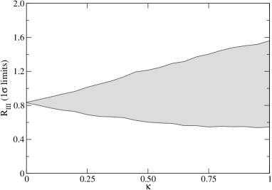
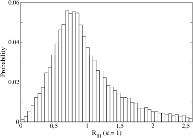
Figure 5: Effect of the random perturbations on the ratio $R_{\mathrm{I\!I\!I}}$, defined in the text.

The plot in Fig. 5 (left) shows that the perturbations change this ratio from an initial value $(R_{\mathrm{I\!I\!I}})_{0}=0.83$ to an interval between $0.55$ and $1.56$. This implies that the corrections to the Yukawa matrices might hide an underlying relation given by Eq. (19). Relation IV is [18]

$$|V_{cb}|=\sqrt{\frac{m_{c}}{m_{t}}}\,.$$ (21)

Correspondingly, we define

$$R_{\mathrm{I\!V}}\equiv\frac{1}{|V_{cb}|}\sqrt{\frac{m_{c}}{m_{t}}}\,.$$ (22)

This quantity is plotted in Fig. 6. Since the ratios $m_{u}/m_{c}$ and $|V_{ub}/V_{cb}|$ are not modified by the random perturbations, the behaviour is similar to $R_{\mathrm{I\!I\!I}}$, up to a global factor.

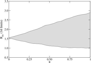
Figure 6: Effect of the random perturbations on the ratio $R_{\mathrm{I\!V}}$, defined in the text.

Relations V and VI [19] are very similar and involve only quark masses:

$$\frac{m_{u}}{m_{c}}=\frac{m_{c}}{m_{t}}~{},~{}~{}~{}\frac{m_{d}}{m_{s}}=\frac{m_{s}}{m_{b}}\,.$$ (23)

The impact of the “anarchy” on them can be investigated with the analysis of the ratios

$$R_{\mathrm{V}}\equiv\frac{m_{u}m_{t}}{m_{c}^{2}}~{},~{}~{}~{}R_{\mathrm{V\!I}}\equiv\frac{m_{d}m_{b}}{m_{s}^{2}}\,,$$ (24)

which are plotted in Figs. 7 and 8, respectively. These quantities are (up to global factors) the inverse of the ratios $m_{c}/m_{t}$ and $m_{s}/m_{b}$ studied above.

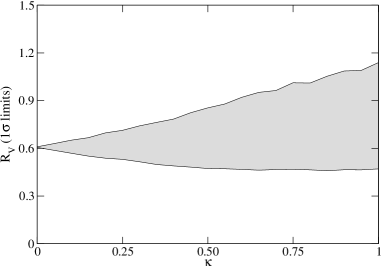
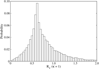
Figure 7: Effect of the random perturbations on the ratio $R_{\mathrm{V}}$, defined in the text.

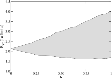
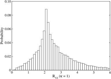
Figure 8: Effect of the random perturbations on the ratio $R_{\mathrm{V\!I}}$, defined in the text.

Relation VII [20, 21] is analogous to Relation $\mathrm{I\!I}$ in Eq. (18),

$$\left|\frac{V_{td}}{V_{ts}}\right|=\sqrt{\frac{m_{d}}{m_{s}}}\,.$$ (25)

Since the ratio $|V_{ub}/V_{cb}|$ and the phase $\delta$ do not change with the perturbations, Relation VII remains inaltered as well. Relation VIII is [20]

$$|V_{cb}|=\sqrt{2}\,\frac{m_{s}}{m_{b}}\,.$$ (26)

In principle, both sides of this equality change when the random perturbations are added to the Yukawa matrices. However, the changes are correlated and the relation is not affected. The same happens with Relation IX [20],

$$|V_{ub}|=\sqrt{\frac{m_{d}m_{s}}{2m_{b}^{2}}}\,.$$ (27)

The non-trivial invariance of these relations under the “anarchy” is due to the formal structure adopted for the latter, Eqs. (6).

As remarked at the beginning of this Section, the test of Relations I–IX must be done at very high energies, where the flavour symmetry originating the Yukawa patterns is not broken. In this context, we would like to point out that the test of Relations I, II, VII, VIII and IX, as well as other relations invariant under random perturbations, can provide a better way to discriminate between different models of Yukawa patterns. On the other hand, Relations III, IV, V and VI can be influenced by radiative corrections from new physics and hence their observation might be unclear.

5 Enhancement of the hierarchy

We want to investigate within our framework to what extent the “anarchy” might contribute to (or even generate) the observed hierarchy of quark masses and mixings. The guideline of our analysis is the following: we reduce the hierarchy in the parameters of the Lagrangian and then calculate the probability that the hierarchy present in the SM is reproduced with the random perturbations. We have studied three examples, corresponding to an enhancement of the hierarchy in the up-type quark masses, down-type quark masses and CKM mixing angles, respectively.

1. In the first case, we use the same parameters as in Section 3 but replace the top mass by $m_{t}^{\prime}=m_{t}/2$. In this situation, the ratio of masses $m_{c}/m_{t}$ is larger by a factor of two, $(m_{c}/m^{\prime}_{t})_{0}=7.7\times 10^{-3}$ (that is, the hierarchy is reduced). Setting $\kappa=1$, we generate a sample of 10000 random Yukawa matrices. A good estimate of the likelihood to enhance the hierarchy is given by the probability that the ratio $m_{c}/m^{\prime}_{t}$ after perturbations is smaller or equal than the value $m_{c}/m_{t}$ obtained with the true top mass. This probability is only $8.3\times 10^{-3}$.

2. In the second example, we use the standard parameters but replace the bottom mass by $m_{b}^{\prime}=m_{b}/2$. With the same procedure, we find that the probability that the ratio $m_{s}/m_{b}^{\prime}$ after random perturbations is smaller or equal to the SM value is $0.12$, more than one order of magnitude larger than in the previous case.

3. In the third example, we use the SM values of the masses, the mixing angle $|V_{us}|$ and the phase $\delta$, multiplying $|V_{ub}|$ and $|V_{cb}|$ by two. The probability that the ratio $|V_{cb}/V_{us}|$ after random perturbations is equal or smaller than the SM value is $0.12$.

With these examples we see that the observed large hierarchy between the second and third generations is not an effect of the “anarchy” (as discussed in Ref. [5]), though for down-type quarks it can receive some enhancements from unknown corrections. The two mixing angles $V_{ub}$, $V_{cb}$ can also be reduced by the corrections.

6 Summary

We have introduced a basis-independent parameterisation in order to describe the effect of unknown corrections from new physics (“anarchy”) in the quark and lepton mass matrices. With this parameterisation we have explored the stability of some properties of the quark Yukawa matrices against unknown corrections. This has been done with the addition of random perturbations to these matrices and a statistical analysis of the effect of the perturbations.

We have shown that the quark mass hierarchies, namely the ratios $m_{u}/m_{c}$, $m_{c}/m_{t}$, $m_{d}/m_{s}$, $m_{s}/m_{b}$ and $m_{b}/m_{t}$ are hardly affected by the random perturbations. Of these quantities, $m_{u}/m_{c}$ and $m_{d}/m_{s}$ remain constant for most of the values of the random parameters. The rest exhibit deviations that in average lead to an enhancement of the original hierarchy, but without modifying it significantly. We have also analysed the effect in the mixing angles, concluding that neither $|V_{us}|$, nor the ratio $|V_{ub}/V_{cb}|$, nor the phase $\delta$ change appreciably with the random perturbations. The mixing angles $|V_{ub}|$ and $|V_{cb}|$ show deviations but still preserving the CKM hierarchy $|V_{us}|\gg|V_{cb}|\gg|V_{ub}|$. For some fine-tuned values of the random parameters, the strong hierarchy of masses and mixing angles is removed, but this only happens in a extremely small subset of the sample. We have also found that when the size of the random perturbations (the $\kappa$ parameter) is increased, the average effects do not grow linearly but their increase rate slows down.

We have selected nine simple flavour relations among quark masses and CKM mixing angles, predicted by several models in the literature, discussing the effect of the “anarchy” on them. We have identified four relations which are affected by the random perturbations. If these relations are fulfilled by the Yukawa matrices, as some theoretical models predict [1, 18, 19], the phenomenological observation may be jeopardised by the “anarchy”: some flavour properties in the Lagrangian might not be apparent and the “anarchy” might blur or hide an underlying flavour relation. On the other hand, the remaining five relations discussed are not altered by the “anarchy” and hence their analysis could provide a cleaner insight into the structure of the Yukawa matrices.

Finally, we have used our framework to demonstrate that the possibility that unknown corrections give large contributions to the hierarchy of masses and mixings is very unlikely, at it has been pointed out before in the literature. We have shown that if, for instance, one enhances the ratio $m_{c}/m_{t}$ in the Yukawa matrices in the Lagrangian (thus reducing the hierarchy), the probability that the corrections bring it down to the SM value is very small.

Acknowledgements

I thank F. del Águila and A. M. Teixeira for a careful reading of the manuscript. This work has been supported by the European Community’s Human Potential Programme under contract HTRN–CT–2000–00149 Physics at Colliders.

References

- [1] P. Ramond, R. G. Roberts and G. G. Ross, Nucl. Phys. B 406 (1993) 19
- [2] H. Harari, H. Haut and J. Weyers, Phys. Lett. B 78 (1978) 459; for a recent analysis see G. C. Branco, M. E. Gómez, S. Khalil and A. M. Teixeira, hep-ph/0204136
- [3] H. Fritzsch, Phys. Lett. 73B (1978) 317
- [4] B. Stech, Phys. Lett. B 130 (1983) 189
- [5] C. D. Froggatt and H. B. Nielsen, Nucl. Phys.B 147 (1979) 277
- [6] R. Rosenfeld and J. L. Rosner, Phys. Lett. B 516 (2001) 408
- [7] S. Fukuda et al. [Super-Kamiokande Collaboration], Phys. Rev. Lett. 86 (2001) 5656
- [8] L. J. Hall, H. Murayama and N. Weiner, Phys. Rev. Lett. 84 (2000) 2572; N. Haba and H. Murayama, Phys. Rev.D 63 (2001) 053010
- [9] G. Altarelli, F. Feruglio and I. Masina, hep-ph/0210342
- [10] T. P. Cheng, E. Eichten and L. F. Li, Phys. Rev. D 9 (1974) 2259
- [11] H. Arason, D. J. Castaño, B. Keszthelyi, S. Mikaelian, E. J. Piard, P. Ramond and B. D. Wright, Phys. Rev. D 46 (1992) 3945
- [12] F. del Aguila, J. A. Aguilar-Saavedra and M. Zralek, Comput. Phys. Commun. 100 (1997) 231
- [13] J. A. Aguilar-Saavedra et al., in preparation
- [14] K. Hagiwara et al., Particle Data Group, Phys. Rev. D 66 (2002) 010001
- [15] J. A. Aguilar-Saavedra and M. Masip, Phys. Rev. D 54 (1996) 6903
- [16] R. Gatto, G. Sartori and M. Tonin, Phys. Lett. B 28 (1968) 128
- [17] R. J. Oakes, Phys. Lett. B 29 (1969) 683
- [18] S. Dimopoulos, L. J. Hall and S. Raby, Phys. Rev. Lett. 68 (1992) 1984; Phys. Rev. D 45 (1992) 4192
- [19] G. C. Branco, D. Emmanuel-Costa and R. González Felipe, Phys. Lett. B 483 (2000) 87
- [20] G. C. Branco, D. Emmanuel-Costa and J. I. Silva-Marcos, Phys. Rev. D 56 (1997) 107
- [21] R. Barbieri, L. J. Hall and A. Romanino, Nucl. Phys. B 551 (1999) 93