Abstract

The spin structure of the nucleon is analyzed in the framework of a Lorentz–invariant formulation of baryon chiral perturbation theory. The structure functions of doubly virtual Compton scattering are calculated to one–loop accuracy (fourth order in the chiral expansion). We discuss the generalization of the Gerasimov–Drell–Hearn sum rule, the Burkhardt–Cottingham sum rule and moments of these. We give predictions for the forward and the longitudinal–transverse spin polarizabilities of the proton and the neutron at zero and finite photon virtuality. A detailed comparison to results obtained in heavy baryon chiral perturbation theory is also given.

1 Introduction and summary

Understanding the spin structure of the nucleon is a central topic of present nuclear and particle physics activities, for a review see [1]. Of particular interest are certain sum rules which connect information at all energy scales, like e.g. the Gerasimov–Drell–Hearn (GDH) sum rule and its generalization to finite photon virtuality or the Burkhardt–Cottingham (BC) sum rule. Such sum rules are interesting from the theoretical point of view because they constitute moments of the sought after nucleon spin structure functions $g_{1}$ and $g_{2}$. On the experimental side challenging new meson production experiments using real or virtual photons play an important role since only recently it has become possible to work with polarized beams and polarized targets, thus offering the possibility of mapping out the nucleons’ spin structure encoded in these two functions, which can be formulated on a purely partonic (high energy regime) or hadronic level (low energy regime). In both these extreme cases, systematic and controlled theoretical calculations can be performed. The region of intermediate momentum transfer is accessible using quark/resonance models or can be investigated using dispersion relations. In fact, one of the final goals of many of these investigations is to obtain an understanding of how in QCD this transition from the non–perturbative to the perturbative regime takes place, guided by the precise experimental mapping of spin–dependent observables from low momentum transfer to the multi–GeV region, as it is one of the main thrusts of the research carried out e.g. at Jefferson Laboratory.

Here we focus on a theoretical investigation of the nucleon’s spin structure in the non-perturbative regime of QCD. We are utilizing chiral perturbation theory (CHPT) to analyze the structure of the nucleon at low energies, based on the spontaneous and explicit chiral symmetry breaking QCD is supposed to undergo (for a general review, see e.g. [2]). By now it is well established that the pion cloud plays an important role in understanding the nucleons properties in the non–perturbative regime of QCD, and many processes have been analyzed using chiral perturbation theory. Some recent work in various versions/extensions of baryon CHPT pertinent to the topics discussed here can be found e.g. in Refs. [3, 4, 5, 6, 7, 8]. In the letter [9] we had presented a novel analysis of chiral loop effects in the generalized Gerasimov–Drell–Hearn sum rule in the framework of a Lorentz–invariant formulation of baryon chiral perturbation theory [10]. We performed a complete one–loop calculation for the spin–dependent proton and neutron structure functions $S_{1,2}(\nu=0,Q^{2})$ of forward double virtual Compton scattering (V²CS), where $\nu$ is the energy transfer and $Q^{2}$ the negative of the photon virtuality (momentum transfer squared). Combining the methods of CHPT and analyticity, one can deduce all desired spin-related sum rules, respectively all moments of the nucleon’s spin structure functions, from these two basic building blocks for $Q^{2}\lesssim 0.3$ GeV². Results where thus presented for the V²CS structure functions $\bar{S}_{1}^{p,n}(0,Q^{2})$ (where the bar indicates the subtraction of the elastic intermediate state) and for the first moment of the sum rule for the spin–dependent structure function $g_{1}$ (for precise definitions, see below). Also, a comparison to the previously obtained so called “heavy baryon” results, which are implicitly contained in our calculation and can be extracted by performing a 1/(nucleon mass) expansion of our relativistic results, was given. Here, in the light of the sometimes rather slowly converging $1/m$ expansion of the heavy baryon framework in the spin sector [9], we do not only give a detailed exposition of how the relativistic results have been obtained, but also give novel results for the structure functions $\bar{S}_{2}^{p,n}(0,Q^{2})$, for the generalization of the DHG and BC sum rules as well as for the forward and longitudinal–transverse spin polarizabilities. These latter two quantities parameterize the forward spin–dependent (virtual) Compton scattering amplitude at low energies and encode important information about higher moments of the nucleon’s spin structure functions.

The pertinent results of this investigation can be summarized as follows:

• We have studied spin–dependent doubly virtual Compton scattering off nucleons to fourth order (one loop) in a Lorentz–invariant formulation of baryon chiral perturbation theory. At this order in the chiral expansion, no unknown low–energy constants appear and thus we obtain parameter–free predictions for the spin structure functions $\bar{S}_{1,2}(\nu,Q^{2})$, where the bar signals the subtraction of the elastic intermediate state. These two V²CS structure functions serve as the fundamental building blocks from which all other results can be derived.

• We have studied the corresponding sum rules (the generalization of the Gerasimov–Drell–Hearn sum rule to finite photon virtuality and the Burkhardt–Cottingham sum rule) and their moments, which can be obtained by expanding the structure functions at low energies $\nu$, cf. Eqs. (2.3,2.29,2.32).

• We have estimated the contribution of $\Delta(1232)$ Born graphs and from vector meson contributions as described in Section 3.3. The delta plays an important role in the nucleon spin sector and thus an extension of our work including $\pi\Delta$ loops in a systematic manner is called for.

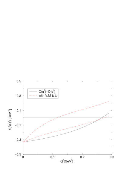
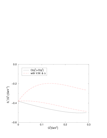
Figure 3: Predictions for the structure function $\bar{S}_{1}({0,Q^{2}})$ with the elastic intermediate state subtracted in units of GeV^-2. The solid lines show the fourth order (one–loop) result whereas the bands given by the dashed lines refer to the one–loop plus resonance (delta Born graphs and vector meson) results. Left (right) panel: Proton (neutron).

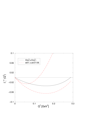
Figure 4: Prediction for the moment $\Gamma_{1}^{p}({Q^{2}})$. The solid lines show the fourth order (one–loop) result whereas the bands given by the dashed lines refer to the one–loop plus resonance (delta Born graphs and vector meson) results. No $N\Delta\gamma$ form factor was used.

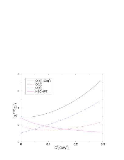
Figure 5: Chiral loop contribution to the first moment $\bar{S}_{1}^{(2)}(0,Q^{2})$ with the elastic contribution subtracted in units of GeV^-4. The solid (dashed/dot-dashed) line gives the result of the present calculation to order $q^{4}$ (the contribution from the third/forth order) in comparison to the heavy baryon result of [6] (dotted line). Left (right) panel: Proton (neutron).

• Results for $\bar{S}_{1}^{p,n}(0,Q^{2})$ and the first moment $\Gamma_{1}^{p,n}(Q^{2})$ as well as for $\Gamma_{1}^{p-n}(Q^{2})$ were already given and discussed in [9]. We note that the prediction for $\Gamma_{1}^{p-n}(Q^{2})$ is free of spin–3/2 effects and in rough agreement with preliminary data from Jefferson Laboratory [11]. Predictions for the structure functions $\bar{S}_{1}^{p,n}(0,Q^{2})$ and for the moment $\Gamma_{1}^{p}(Q^{2})$ including resonance contributions, as well as for the chiral expansion of the second moments $\bar{S}_{1}^{(2)p,n}(0,Q^{2})$ are shown in Fig. 3, Fig. 4 and Fig. 5, respectively.

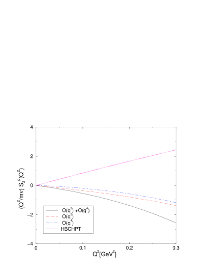
Figure 6: Chiral loop contribution to the structure function $(Q^{2}/m\nu)\bar{S}_{2}(0,Q^{2})|_{\nu=0}$ with the elastic contribution subtracted in units of GeV^-2. The solid (dashed/dot-dashed) line gives the result of the present calculation to order $q^{4}$ (the contribution from the third/forth order) in comparison to the heavy baryon result of [6] (dotted line). Left (right) panel: Proton (neutron).

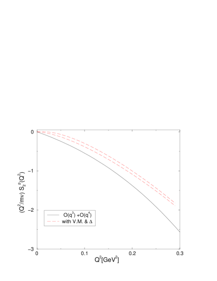
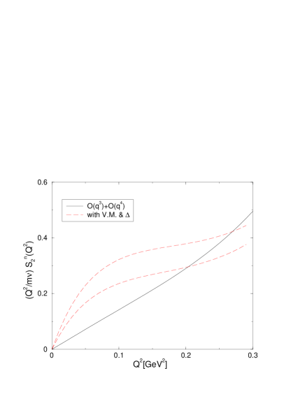
Figure 7: Chiral loop (solid line) and one–loop plus resonance contributions (dashed lines) to the structure function $(Q^{2}/m\nu)\bar{S}_{2}(0,Q^{2})|_{\nu=0}$ with the elastic contribution subtracted in units of GeV^-2. Left (right) panel: Proton (neutron).

• The one–loop results for the second structure function are shown in Fig. 6 for the proton and the neutron. They come out sizeably different from the heavy baryon result for the same reasons as already discussed in [9] in connection with the first structure function. The delta Born and vector meson contributions have also been evaluated, see Fig. 7.

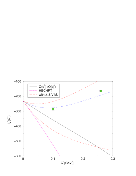
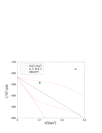
Figure 8: The integral $I_{A}(Q^{2})$ for the neutron in units of $\mu$b. The solid line gives the fourth order result, the dashed lines represent the theoretical uncertainty due to variation in the delta parameters as explained in Section 3.3. For comparison, the HBCHPT result is depicted by the dotted line. The data are from Ref. [12]. Note that here we have adjusted our normalization to the one used by the experimentalists. Left (right) panel: Without (with) $\Delta N\gamma$ form factor. The dot–dashed line in the left panel corresponds to the delta parameters $g_{2}=9.5$, $X=Y=-0.725$ as discussed in the text.

• The chiral prediction for a linear combination of first moments of $g_{1}$ and $g_{2}$ commonly denoted as $I_{A}^{n}(Q^{2})$ supplemented with resonance contributions (mostly from the delta) agrees with recent data from Jefferson Laboratory [12] for virtualities $Q^{2}\lesssim 0.3\,$GeV², see Fig. 8. However, if one includes a $\Delta N\gamma$ vertex function as suggested by older electroproduction data at higher energies, one is not able to describe the curvature of the data as the virtuality increases, see also Fig. 8.

• The Burkhardt–Cottingham sum rule is fulfilled within the Lorentz–invariant approach used here. However, truncating the product of form factors at fourth order does not give a very accurate representation of the full result, which can be obtained using the form factors from dispersion theory or infrared regularized baryon CHPT supplemented by vector mesons [13].

• We have calculated the forward spin polarizability $\gamma_{0}(Q^{2})$ (which corresponds to a linear combination of the second moments of $g_{1}$ and $g_{2}$) at zero and finite photon virtuality to ${\cal O}(p^{4})$ in relativistic baryon CHPT for the proton and the neutron. To obtain a reliable prediction for the chiral corrections to these spin polarizabilities at $Q^{2}=0$ in the heavy baryon approach, we find that one has to account (at least) for terms of ${\cal O}(M_{\pi})$, i.e. go to N⁴LO in the calculation. However, we note that even our relativistic one-loop result, when supplanted with resonance model delta Born term and vector meson contributions, still does not agree with the data [14]. We have also isolated the reason for the bad convergence, it rests entirely on the slow convergence of the pole (Born) graphs.

• We have calculated the longitudinal–transverse spin polarizability $\delta_{0}(Q^{2})$ (which corresponds to a linear combination of the second moment of $g_{1}$ and the first moment of $g_{2}$) at zero and finite photon virtuality for proton and neutron. When performing a chiral expansion on the full relativistic results, including terms up–to–and–including ${\cal O}(M_{\pi})$, one finds a good convergence for these quantities at the photon point in the $1/m$ expansion. This observation and the absence of large delta (Born-term) contributions leads to the hope that $\delta_{0}(Q^{2})$ can serve as a testing ground of the chiral dynamics of QCD which might be better suited than the forward spin polarizabilities of the nucleon.

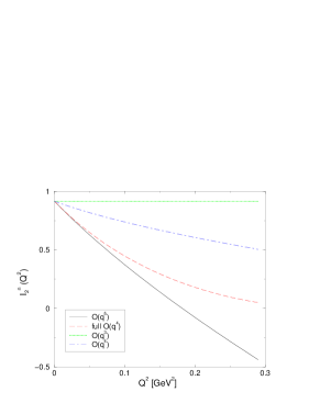
Figure 14: The integral $I_{2}(Q^{2})$ for the neutron. The dashed lines represents the full fourth order results (that is the form factors taken to fourth order). The solid/dot-dashed/dotted line gives the fifth/fourth/third order result (i.e. the product of the form factors taken to that order).

• We have calculated the fifth order contributions from the pole (Born) graphs for a particular combination of the structure functions of the neutron shown in Fig. 13. The complete fifth order result for the neutron BC sum rule is in good agreement with the product of the form factors for $Q^{2}\lesssim 0.15\,$GeV², cf. Fig. 14. The partial fifth order contribution to the neutron’s spin polarizability is non–negligible and negative, indicating that these terms might be the origin for explaining the discrepancy to the data in case of the proton.

The material in this paper is organized as follows. Section 2 contains the basic formalism for spin-dependent doubly virtual Compton scattering off nucleons, its relation to pion electroproduction and the derivation of the pertinent sum rules and their moments. In section 3, the theory underlying our calculations is exposed together with the chiral expansion of the spin–dependent structure functions. We also show how we estimate various resonance contributions. The results are presented and discussed in section 4. Some technicalities are relegated to the appendix.

2 Basic formalism

This section contains the basic formalism on spin-dependent doubly virtual Compton scattering off nucleons, its relation to inelastic electroproduction and the derivation of the corresponding sum rules. The reader familiar with these concepts might directly proceed to section 3.

2.1 Doubly virtual Compton scattering

We consider spin–dependent doubly virtual Compton scattering (V²CS) off nucleons (neutrons or protons) in forward direction, that is the reaction

$$\gamma^{\star}(q,\epsilon)+N(p,s)\to\gamma^{\star}(q,\epsilon^{\prime})+N(p,s^{\prime})~{},$$ (2.1)

with $q~{}(p)$ the virtual photon (nucleon) four–momentum, $s~{}(s^{\prime})$ the nucleon spin (polarization) and $\epsilon\,(\epsilon^{\prime})$ the polarization four–vector of the incoming (outgoing) photon. It is common to express the spin amplitude of V²CS in terms of two structure functions, called $S_{1}(\nu,Q^{2})$ and $S_{2}(\nu,Q^{2})$, via

$$T^{[\mu\nu]}(p,q,s)=-i\;\frac{m}{N}\,\epsilon^{\mu\nu\alpha\beta}q_{\alpha}\left\{s_{\beta}\,S_{1}(\nu,Q^{2})+\left[p\cdot q\,s_{\beta}-s\cdot q\;p_{\beta}\right]\frac{S_{2}(\nu,Q^{2})}{m^{2}}\right\},$$ (2.2)

where $s^{\mu}$ denotes a spin-polarization four-vector, $m$ is the nucleon mass, $\epsilon^{\mu\nu\alpha\beta}$ the totally antisymmetric Levi–Civita tensor with $\epsilon^{0123}=1$, $\nu=p\cdot q/m$ the energy transfer and $Q^{2}=-q^{2}\geq 0$ the (negative of the) photon virtuality. $N$ is a convention dependent normalization factor. Following Ref.[9] we set $S_{1}(0,0)=-e^{2}\,\kappa^{2}/m^{2}$. With the spinor normalization $\bar{u}u=1$ typically used in baryon CHPT, we find $N=2m$, which we will utilize throughout this work. Note that while $S_{1}(\nu,Q^{2})$ is even under crossing $\nu\leftrightarrow-\nu$, the structure function $S_{2}(\nu,Q^{2})$ is odd.

In the rest frame of the nucleon the forward virtual Compton tensor in the Coulomb gauge $\epsilon_{0}=\epsilon^{\prime}_{0}=0$ simplifies to

$$T^{[ij]}_{\rm rest}(\nu,Q^{2})=\frac{i}{2}\;\epsilon_{ijk}\chi^{\dagger}\left\{\nu\,\sigma^{k}S_{1}(\nu,Q^{2})+\left[\nu^{2}\sigma^{k}-\sigma\cdot q\,q^{k}\right]\frac{S_{2}(\nu,Q^{2})}{m}\right\}\chi~{},$$ (2.3)

where $\nu$ now corresponds to the photon energy in the laboratory system, the $\sigma_{k}$ $(k=1,2,3)$ are the Pauli spin–matrices and $\chi$ is a two-component spinor. Utilizing the identity

$$\vec{\sigma}\cdot\vec{q}\,\vec{\epsilon}^{\,\prime}\cdot(\vec{\epsilon}\times\vec{q})=\left(\nu^{2}+Q^{2}\right)\left[\vec{\sigma}\cdot(\vec{\epsilon}^{\,\prime}\times\vec{\epsilon})-\left(\vec{\sigma}\cdot(\vec{\epsilon}^{\,\prime}\times\hat{q})\,\vec{\epsilon}\cdot\hat{q}-\vec{\sigma}\cdot(\vec{\epsilon}\times\hat{q})\,\vec{\epsilon}^{\,\prime}\cdot\hat{q}\right)\right]$$ (2.4)

we finally arrive at the V²CS forward matrix element

$$\epsilon^{\prime}\cdot T\cdot\epsilon|_{\rm rest} = \frac{1}{2m}\,\chi^{\dagger}\left\{i\vec{\sigma}\cdot\left(\vec{\epsilon}^{\,\prime}\times\vec{\epsilon}\right)\left[m\nu S_{1}(\nu,Q^{2})-Q^{2}S_{2}(\nu,Q^{2})\right]\right.$$ (2.5)

$$\phantom{\frac{1}{N}\;\chi^{\dagger}}\left.+i\left[\vec{\sigma}\cdot(\vec{\epsilon}^{\,\prime}\times\hat{q})\,\vec{\epsilon}\cdot\hat{q}-\vec{\sigma}\cdot(\vec{\epsilon}\times\hat{q})\,\vec{\epsilon}^{\,\prime}\cdot\hat{q}\right]\left(\nu^{2}+Q^{2}\right)S_{2}(\nu,Q^{2})\right\}\chi\;,$$

in the form which is best suited for our calculations in the framework of relativistic baryon chiral perturbation theory. The Compton amplitudes $S_{1,2}(\nu,Q^{2})$ are amenable to a chiral expansion as will be detailed in section 3. We remark that in what follows, we will mostly be concerned with the reduced amplitudes

$$\bar{S}_{i}(\nu,Q^{2})=S_{i}(\nu,Q^{2})-S_{i}^{\rm el}(\nu,Q^{2})~{},$$ (2.6)

i.e. the Compton amplitudes with the contribution from the elastic intermediate state subtracted. More precisely, these are the contributions from the single nucleon exchange (pole) terms with the corresponding vertices given in terms of the electromagnetic form factors. Only the non-pole parts of the corresponding diagrams contribute to the nucleon spin structure as discussed in more detail below. We note that for the calculations to follow we mostly work at $\nu=0$ (and therefore often do not make explicit the energy dependence of certain quantities). In fact, for the calculations we make use of crossing symmetry, which allows to write the relativistic V²CS forward matrix element in terms of two invariant functions $A(\nu,Q^{2})$ and $B(\nu,Q^{2})$ as:

$$\epsilon^{\prime}\cdot T\cdot\epsilon|_{\rm rest} = \chi^{\dagger}\left\{i\vec{\sigma}\cdot\left(\vec{\epsilon}^{\,\prime}\times\vec{\epsilon}\right)\left[A(s,Q^{2})-A(2m^{2}-2Q^{2}-s,Q^{2})\right]\right.$$

$$+ \left.i\left[\vec{\sigma}\cdot(\vec{\epsilon}^{\,\prime}\times\hat{q})\,\vec{\epsilon}\cdot\hat{q}-\vec{\sigma}\cdot(\vec{\epsilon}\times\hat{q})\,\vec{\epsilon}^{\,\prime}\cdot\hat{q}\right]\,|\vec{q}\,|^{2}\,\left[B(s,Q^{2})-B(2m^{2}-2Q^{2}-s,Q^{2})\right]\right\}\chi\;,$$

with $s=(p+q)^{2}$ the standard Mandelstam variable, which is related to $\nu$ via $\nu=(s-m^{2}+Q^{2})/2m$. Written in term of $\nu$, crossing symmetry means that in this equation the difference of a quantity taken at $\nu$ with the same quantity taken at $-\nu$ appears. Since we consider quantities at $\nu=0$ i.e. at $s=m^{2}+q^{2}$, all of these can be obtained as derivatives of order $n\geq 1$ of the functions $A$ and $B$. More precisely, we give two examples to illustrate this method,

$$\bar{S}_{1}(0,Q^{2})-{Q^{2}\over m}\lim_{\nu\to 0}{\bar{\underline{S}}_{2}(0,Q^{2})\over\nu} = 4\,{dA(\nu,Q^{2})\over d\nu}\bigg{|}_{\nu=0}~{},$$ (2.8)

$$Q^{2}\lim_{\nu\to 0}{\bar{\underline{S}}_{2}(0,Q^{2})\over\nu} = 4\,{dB(\nu,Q^{2})\over d\nu}\bigg{|}_{\nu=0}~{},$$ (2.9)

where $\nu\bar{\underline{S}}_{2}(\nu,Q^{2})=\nu\bar{S}_{2}(\nu,Q^{2})-\nu\bar{S}_{2}(\nu,Q^{2})\big{|}_{\nu=0}\,$.

2.2 Relation to inelastic electroproduction off nucleons

Because of unitarity, there is a basic connection between spin structure functions in V²CS and the ones probed in inelastic electroproduction experiments. This is simply related to the fact that the imaginary part of the Compton tensor is given in terms of nucleon plus meson states, the lowest one being the pion–nucleon state. The differential cross section for exclusive electroproduction can be expressed in terms of four virtual photoabsorption cross sections $\sigma_{T}(\nu,Q^{2})$, $\sigma_{L}(\nu,Q^{2})$, $\sigma_{LT}^{\prime}(\nu,Q^{2})$ and $\sigma_{TT}^{\prime}(\nu,Q^{2})$. The transverse, $\sigma_{T}$, and the transverse–transverse, $\sigma_{TT}^{\prime}$, cross sections can be related to the total photoabsorption cross sections $\sigma_{1/2}$ and $\sigma_{3/2}$ corresponding to the excitation of intermediate states with spin projection 3/2 and 1/2, respectively:

$$\sigma_{T}={1\over 2}\left(\sigma_{3/2}+\sigma_{1/2}\right)~{},$$ (2.10)

(2.11)

$$\sigma_{TT}^{\prime}={1\over 2}\left(\sigma_{3/2}-\sigma_{1/2}\right)~{}.$$ (2.12)

The four virtual photoabsorption cross sections are related to the quark structure functions $F_{1}$, $F_{2}$, $G_{1}$ and $G_{2}$ (that depend on $\nu$ and $Q^{2}$) measured in (un)polarized deep inelastic electron scattering off nucleons via:

$$\sigma_{T}(\nu,Q^{2}) = {4\pi^{2}\alpha\over mK}F_{1}(\nu,Q^{2})~{},$$ (2.13)

$$\sigma_{L}(\nu,Q^{2}) = {4\pi^{2}\alpha\over K}\Bigl{[}{F_{2}(\nu,Q^{2})\over\nu}(1+\gamma^{2})-{F_{1}(\nu,Q^{2})\over m}\Bigr{]}~{},$$ (2.14)

$$\sigma_{LT}^{\prime}(\nu,Q^{2}) = -{4\pi^{2}\alpha\over K}\,\gamma\;\nu\;(G_{1}(\nu,Q^{2})+{\nu\over m}G_{2}(\nu,Q^{2}))~{},$$ (2.15)

$$\sigma_{TT}^{\prime}(\nu,Q^{2}) = -{4\pi^{2}\alpha\over K}\,\nu\;(G_{1}(\nu,Q^{2})-{\nu\over m}\gamma^{2}G_{2}(\nu,Q^{2}))~{},$$ (2.16)

where $\nu=E-E^{\prime}$ is the virtual photon energy in the lab frame, $\alpha=e^{2}/4\pi=1/137.036$ the fine structure constant, $\gamma=Q/\nu$ and $K$ a flux factor. For more details on the electroproduction formalism, see e.g. Ref.[16].

2.3 Sum rules and moments

Let us first consider the real photon case with $Q^{2}=0$. At low energies one expands the coefficient

$$2\,m\,g(\nu)=\lim_{Q^{2}\to 0}m\nu S_{1}(\nu,Q^{2})-Q^{2}S_{2}(\nu,Q^{2})$$ (2.17)

in front of the spin-dependent operator $\vec{\sigma}\cdot\left(\vec{\epsilon}^{\,\prime}\times\vec{\epsilon}\,\right)$ in powers of the energy transfer,

$$g(\nu)=-{e^{2}\kappa^{2}\over 2m^{2}}\nu+4\pi\;\gamma_{0}\;\nu^{3}+{\cal O}(\nu^{5})~{},$$ (2.18)

where the first term proportional to the nucleon anomalous magnetic moment squared ($\sim\kappa^{2}$) is given by the venerable low–energy theorem (LET) of Low, Gell-Mann and Goldberger [17] and $\gamma_{0}$ is the forward spin polarizability. The imaginary part of $g(\nu)$ can be related via the optical theorem to $\sigma_{1/2}$ and $\sigma_{3/2}$,

$${\rm Im}\;g(\nu)={\nu\over 2}\left(\sigma_{1/2}(\nu,Q^{2}=0)-\sigma_{3/2}(\nu,Q^{2}=0)\right)$$ (2.19)

Writing an unsubtracted dispersion relation for $g(\nu)$ one obtains using Eq.(2.18) and (2.19) the celebrated Drell–Hearn–Gerasimov sum rule [18] (we give here the generic form without specifying whether we mean the neutron or the proton):

$$-{2\;\pi^{2}\;\alpha\;\kappa^{2}\over m^{2}}=\int{d\nu\over\nu}\,\left[\sigma_{3/2}-\sigma_{1/2}\right]~{}.$$ (2.20)

The value of the LHS of the sum rule is $-204\,\mu$b for the proton and $-232\,\mu$b for the neutron. This sum rule is presently under active experimental investigation at MAMI, ELSA, GRAAL, CEBAF and Spring-8. For first results, see [19].

The DHG sum rule has been generalized to finite $Q^{2}$ [20]. It is most natural to connect such a generalization of the sum rule to the Bjorken sum rule in deep inelastic scattering. One thus defines

$$I_{1}(Q^{2})={2m^{2}\over Q^{2}}\int_{0}^{x_{0}}g_{1}(x,Q^{2})dx~{},$$ (2.21)

with $x_{0}$ corresponding to the pion production threshold. Here, $G_{1}=g_{1}/(m\nu)$ can be related to $\sigma_{3/2}$ and $\sigma_{1/2}$ via Eqs.(2.10,2.16) and $x=Q^{2}/2m\nu$ is the standard scaling variable. At zero virtuality, one recovers the DHG sum rule, i.e. $I_{1}(0)=-\kappa^{2}/4$. Similarly, there exists a sum rule for the second spin structure function, $g_{2}$, the so–called Burkhardt–Cottingham (BC) sum rule [21]:

$$I_{2}(Q^{2}) = {2m^{2}\over Q^{2}}\int_{0}^{x_{0}}g_{2}(x,Q^{2})dx$$ (2.22)

$$= {1\over 4}{G_{M}(Q^{2})-G_{E}(Q^{2})\over(1+{Q^{2}\over 4m^{2}})}G_{M}(Q^{2})={1\over 4}F_{2}(Q^{2})\,\left(F_{1}(Q^{2})+F_{2}(Q^{2})\right)~{},$$ (2.23)

where $G_{E}(Q^{2})$ and $G_{M}(Q^{2})$ are the electric and the magnetic nucleon Sachs form factor, respectively, $F_{1}(Q^{2})$ and $F_{2}(Q^{2})$ are the Dirac and the Pauli form factor, in order, and $G_{2}=g_{2}/\nu^{2}$. We note that in a Lorentz-invariant calculation as performed here, the Dirac and Pauli form factors appear naturally, while in the HBCHPT approach the Sachs form factors are the more appropriate quantities [22]. This sum rule assumes that $\sigma_{LT}^{\prime}$ vanishes faster than $1/\nu$ at large $\nu$. Other sum rules have been defined in the literature, see e.g. [3, 16]:

$$I_{A}(Q^{2}) = {2m^{2}\over Q^{2}}\int_{0}^{x_{0}}(g_{1}(x,Q^{2})-\gamma^{2}g_{2}(x,Q^{2}))dx~{},$$ (2.24)

$$I_{C}(Q^{2}) = {2m^{2}\over Q^{2}}\int_{0}^{x_{0}}{1\over(1-x)}(g_{1}(x,Q^{2})-\gamma^{2}g_{2}(x,Q^{2}))dx~{}.$$ (2.25)

All these sum rules can be written in terms of the structure functions ${S}_{1}(\nu,Q^{2}),\;{S}_{2}(\nu,Q^{2})$ of V²CS using the following dispersion relations :

$${S}_{1}(\nu,Q^{2}) = 4e^{2}\int_{Q^{2}/2m}^{\infty}\frac{d\nu^{\prime}\nu^{\prime}G_{1}(\nu^{\prime},Q^{2})}{\nu^{\prime 2}-\nu^{2}}~{},$$

$$\nu{S}_{2}(\nu,Q^{2}) = 4e^{2}\int_{Q^{2}/2m}^{\infty}\frac{d\nu^{\prime}\nu^{2}G_{2}(\nu^{\prime},Q^{2})}{\nu^{\prime 2}-\nu^{2}}\;.$$ (2.26)

where use has been made of the optical theorem,

$${\rm Im}~{}{S}_{i}(\nu,Q^{2})=2\pi~{}G_{i}(\nu,Q^{2})~{},\quad(i=1,2)~{}.$$ (2.27)

Expanding the structure functions at low energies $\nu$, that is around $\nu=0$ (note that we now consider the structure functions with the elastic intermediate state subtracted),

$$\bar{S}_{1}(\nu,Q^{2}) = \bar{S}_{1}^{(0)}(0,Q^{2})+\nu^{2}\,\bar{S}_{1}^{(2)}(0,Q^{2})+\nu^{4}\,\bar{S}_{1}^{(4)}(0,Q^{2})+\dots~{},$$

$$\nu\bar{S}_{2}(\nu,Q^{2}) = \bar{S}_{2}^{(-1)}(0,Q^{2})+\nu^{2}\,\bar{S}_{2}^{(1)}(0,Q^{2})+\nu^{4}\,\bar{S}_{2}^{(3)}(0,Q^{2})+\nu^{5}\,\bar{S}_{2}^{(5)}(0,Q^{2})+\dots\;,$$ (2.28)

where the ellipsis denote terms of higher order in $\nu$, one obtains the following set of sum rules for $\bar{S}_{1}(0,Q^{2})$:

$$\bar{S}_{1}^{(0)}(0,Q^{2}) = 4e^{2}\int_{\nu_{0}}^{\infty}\frac{d\nu^{\prime}G_{1}(\nu^{\prime},Q^{2})}{\nu^{\prime}}={4e^{2}\over m^{2}}I_{1}(Q^{2})~{},$$ (2.29)

$$\bar{S}_{1}^{(2i)}(0,Q^{2}) = 4e^{2}\int_{\nu_{0}}^{\infty}\frac{d\nu^{\prime}G_{1}(\nu^{\prime},Q^{2})}{\nu^{\prime(2i+1)}}\quad(i=1,2,3,\dots)~{},$$ (2.30)

noting that $\bar{S}_{1}^{(0)}(0,Q^{2})$ is directly related to $I_{1}(Q^{2})$. Note that the often used first moment $\Gamma_{1}(Q^{2})$ is related to $I_{1}(Q^{2})$ via

$$\Gamma_{1}(Q^{2})=\frac{Q^{2}}{2m^{2}}\,{I}_{1}(Q^{2})~{}.$$ (2.31)

Likewise, $\bar{S}_{2}^{(i)}(0,Q^{2})$ satisfies:

$$\bar{S}_{2}^{(-1)}(0,Q^{2}) = 4e^{2}\int_{\nu_{0}}^{\infty}d\nu^{\prime}G_{2}(\nu^{\prime},Q^{2})={4\over m^{2}}I_{2}(Q^{2})~{},$$ (2.32)

$$\bar{S}_{2}^{(i)}(0,Q^{2}) = 4e^{2}\int_{\nu_{0}}^{\infty}\frac{d\nu^{\prime}G_{2}(\nu^{\prime},Q^{2})}{\nu^{\prime(i+1)}}\quad(i=1,3,5,\ldots)~{},$$ (2.33)

where $\bar{S}_{2}^{(-1)}(0,Q^{2})$ is related to $I_{2}$. In order to calculate $I_{C}$ it is necessary to define a new quantity $\bar{S}_{R}$ similar to $\bar{S}_{1}-Q^{2}\bar{S}_{2}/\nu$, but having only right hand cuts:

$$\bar{S}_{R}(\nu,Q^{2})=4e^{2}\int_{\nu_{0}}^{\infty}d\nu^{\prime}{G_{1}(\nu^{\prime},Q^{2})-Q^{2}G_{2}(\nu^{\prime},Q^{2})/\nu\over\nu^{\prime}-\nu}~{},$$ (2.34)

so that the following relations hold:

$$I_{A}(Q^{2}) = {m^{2}\over 4}\left(\bar{S}_{1}^{(0)}(0,Q^{2})-Q^{2}\bar{S}_{2}^{(1)}(0,Q^{2})\right)~{},$$ (2.35)

$$I_{C}(Q^{2}) = {m^{2}\over 4}\bar{S}_{R}(Q^{2}/2m,Q^{2})~{}.$$ (2.36)

In Eq.(2.18) the forward spin polarizability appears [22], which is defined in terms of the transverse–transverse photoabsorption cross section as

$$\gamma_{0}={1\over 4\pi^{2}}\int{d\nu\over\nu^{3}}(1-x)(\sigma_{1/2}(\nu,0)-\sigma_{3/2}(\nu,0))~{}.$$ (2.37)

Note that $x$ is trivially zero at vanishing virtuality in this equation so that one recovers the usual dispersion relation for $\gamma_{0}$. One can define a similar quantity involving $\sigma^{\prime}_{LT}$ instead of $\sigma_{TT}^{\prime}$, the so–called longitudinal-transverse polarizability, denoted $\delta_{0}$ in what follows,

$$\delta_{0}={1\over 2\pi^{2}}\int{d\nu\over\nu^{3}}(1-x)\lim_{Q^{2}\to 0}\biggl{(}{\nu\over Q}(\sigma_{1/2}(\nu,0)\biggr{)}~{}.$$ (2.38)

These two quantities can be generalized to finite $Q^{2}$. The quantity $x$ was in fact introduced in order to get straightforward relations between $\gamma_{0}(Q^{2})$, $\delta_{0}(Q^{2})$ and the $\bar{S}_{i}(\nu,Q^{2})$. One has:

$$\gamma_{0}(Q^{2}) = {1\over 8\pi}\left(\bar{S}_{1}^{(2)}(0,Q^{2})-\frac{Q^{2}}{m}\bar{S}_{2}^{(3)}(0,Q^{2})\right)~{},$$ (2.39)

$$\delta_{0}(Q^{2}) = {1\over 8\pi}\left((\bar{S}_{1}^{(2)}(0,Q^{2})+\bar{S}_{2}^{(1)}(0,Q^{2})\right)~{}.$$ (2.40)

3 Chiral expansion of the structure functions

Our calculations are based on an effective chiral pion–nucleon Lagrangian in the presence of external sources (like e.g. photons) supplemented by a power counting in terms of quark (meson) masses and small external momenta. Its generic form consists of a string of terms with increasing chiral dimension,

$${\cal L}_{\rm eff}={\cal L}_{\pi N}^{(1)}+{\cal L}_{\pi N}^{(2)}+{\cal L}_{\pi N}^{(3)}+{\cal L}_{\pi N}^{(4)}+{\cal L}_{\pi\pi}^{(2)}+{\cal L}_{\pi\pi}^{(4)}+\ldots~{}.$$ (3.1)

The superscript denotes the power in the genuine small parameter $q$ (denoting pion masses and/or external momenta). A complete one–loop (fourth order) calculation must include all tree level graphs with insertions from all terms given in Eq. (3.1) and loop graphs with at most one insertion from ${\cal L}_{\pi N}^{(2)}$. The complete Lagrangian to this order is given in [23]. We note that for the case under consideration the only appearing dimension two low–energy constants (LECs), called $c_{6}$ and $c_{7}$ [2], can be fixed from the anomalous magnetic moment of the proton and of the neutron, respectively. As discussed below, there are no contributions from ${\cal L}_{\pi N}^{(3,4)}$ for the observables considered here. Besides these chiral corrections to V²CS, we also estimate various resonance contributions to the observables, however, we do not have an equally systematic framework at our disposal for that task. So some future work should be undertaken to sharpen this part of our calculation by e.g. extending the small scale expansion of [25] to Lorentz–invariant formulation.

3.1 Essentials of Lorentz-invariant baryon CHPT

Baryon chiral perturbation theory is complicated by the fact that the nucleon mass does not vanish in the chiral limit and thus introduces a new mass scale apart from the one set by the quark masses. Therefore, any power of the quark masses can be generated by chiral loops in the nucleon (baryon) case, spoiling the one–to–one correspondence between the loop expansion and the one in the small parameter $q$. One method to overcome this is the heavy mass expansion (called heavy baryon chiral perturbation theory, for short HBCHPT) where the nucleon mass is transformed from the propagator into a string of vertices with increasing powers of $1/m$. Then, a consistent power counting emerges. However, this method has the disadvantage that certain types of diagrams are at odds with strictures from analyticity. The best example is the so–called triangle graph, which enters e.g. the scalar form factor or the isovector electromagnetic form factors of the nucleon. In a fully relativistic treatment, such constraints from analyticity are automatically fulfilled. It was recently argued in [24] that relativistic one–loop integrals can be separated into “soft” and “hard” parts. While for the former the power counting as in HBCHPT applies, the contributions from the latter can be absorbed in certain LECs. In this way, one can combine the advantages of both methods. A more formal and rigorous implementation of such a program was given in [10]. The underlying method is called “infrared regularization”. Any dimensionally regularized one–loop integral $H$ is split into an infrared singular (called $I$) and a regular part (called $R$) by a particular choice of Feynman parameterization,

$$H=I+R~{}.$$ (3.2)

Consider first the regular part. If one chirally expands the contributions to $R$, one generates polynomials in momenta and quark masses. Consequently, to any order, $R$ can be absorbed in the LECs of the effective Lagrangian. On the other hand, the infrared (IR) singular part has the same analytical properties as the full integral $H$ in the low–energy region and its chiral expansion leads to the non–trivial momentum and quark–mass dependences of CHPT, like e.g. the chiral logs or fractional powers of the quark masses. For a typical one–loop integral (like e.g. the nucleon self–energy $\Sigma$) this splitting can be achieved in the following way (omitting prefactors)

$$\Sigma=\int\frac{d^{d}k}{(2\pi)^{d}}{1\over AB} = \int_{0}^{1}dz\int\frac{d^{d}k}{(2\pi)^{d}}{1\over[(1-z)A+zB]^{2}}$$ (3.3)

$$= \biggl{\{}\int_{0}^{\infty}-\int_{1}^{\infty}\biggr{\}}dz\int\frac{d^{d}k}{(2\pi)^{d}}{1\over[(1-z)A+zB]^{2}}=I+R~{},$$

with $A=M_{\pi}^{2}-k^{2}-i\epsilon$, $B=m^{2}-(p-k)^{2}-i\epsilon$, $\epsilon\to 0^{+}$, $M_{\pi}$ the pion mass and $d$ the number of space–time dimensions. Any general one–loop diagram with arbitrary many insertions from external sources can be brought into this form by combining the propagators to a single pion and a single nucleon propagator. It was also shown that this procedure leads to a unique, i.e. process–independent result, in accordance with the chiral Ward identities of QCD [10]. Consequently, the transition from any one–loop graph $H$ to its IR singular piece $I$ defines a symmetry–preserving regularization. For more details, the reader is referred to [10].

There is one special feature to IR regularized baryon CHPT that we have to discuss. Here, we are interested in extending the range of photon virtualities $Q^{2}$ to values that eventually allow a matching to the perturbative QCD calculations. However, there is a generic limit to such an extension. A priori, infrared regularization defines a low energy effective field theory, but due to the resummation of kinetic energy insertions and similar effects, one might hope to extend this framework to higher virtualities than the HBCHPT scheme (this expectation was borne out explicitely in the calculation of the neutron charge form factor, see [13]). Consider now a specific one–loop function in $d$ dimensions

$$\Gamma_{0}(s,Q^{2})={1\over i}\,\int{d^{d}l\over(2\pi)^{d}}\,{1\over(M_{\pi}^{2}-l^{2})\,(m^{2}-(p+q-l)^{2})\,(m^{2}-(p-l)^{2})}~{},$$ (3.4)

with $(p+q)^{2}=s$ and $p^{2}=m^{2}$. In infrared regularization, this integral is written as

$$\Gamma_{0}(s,Q^{2})=\Gamma\left(3-\frac{d}{2}\right)\,\int_{0}^{1}\,dy\,\int_{0}^{\infty}\,dz\,z\,C^{\frac{d}{2}-3}(y,z)~{},$$ (3.5)

with $C$ a polynom in $y$ and $z$,

$$C = A\,z^{2}+B\,z+\mu^{2}~{},$$

$$A = 1+2\,y\,\Omega\,\mu+y\,\mu^{2}-y\,(1-y)\,\tau~{},$$

$$B = -2\,y\,\Omega\,\mu-(1+y)\,\mu^{2}~{},$$ (3.6)

and

$$\Omega={s-m^{2}-M_{\pi}^{2}\over 2mM_{\pi}}~{},\quad\mu={M_{\pi}\over m}~{},\quad\tau={q^{2}\over m^{2}}=-{Q^{2}\over m^{2}}~{}.$$ (3.7)

The $\Gamma$–function in Eq.(3.5) contains the pole as $d\to 4$ which has to be dealt with in standard fashion. We also work with the standard value of the scale of dimensional regularization setting $\lambda=m$. All quantities considered here contain derivatives with respect to $s$ of such loop functions at $s=m^{2}+q^{2}\leq m^{2}$ (see the discussion at the end of Section 2.1). At that point,

$$A=1+y\,\tau-y\,(1-y)\,\tau=1+y^{2}\,\tau~{},$$ (3.8)

so that $A=0$ for $\tau=-1/y^{2}$. Consequently, $\Gamma_{0}(s,Q^{2})$ does not converge for $|\tau|\geq 1$. Thus, the photon virtuality is bounded by the nucleon mass. In fact, for higher derivatives the influence of this singularity is felt at smaller values of $Q^{2}$ so that we restrict the range of photon virtualities to $Q^{2}_{\rm max}=0.3\ldots 0.5\,$GeV² depending on the observable one looks at.

3.2 Structure functions

Within this approach, we have calculated the reduced structure functions $\bar{S}_{1,2}^{(p,n)}(0,Q^{2})$, generically called ${\cal S}$ in this section. The chiral expansion of ${\cal S}$ takes the form

$$\bar{\cal S}=\bar{\cal S}^{\rm tree}+\bar{\cal S}^{\rm loop}~{}.$$ (3.9)

In our case, the tree level contribution stems from the remainder of the Born graphs which lead to the following amplitudes (we omit writing down the crossed term contributions)

$$T^{\rm Born}={C(Q^{2})\over s-m^{2}}+{\cal R}~{},$$ (3.10)

with $s=(p+q)^{2}$, $C(Q^{2})$ can be expressed in terms of the nucleon electromagnetic form factors and ${\cal R}$ denotes the non–pole (polynomial) remainder from the Born diagrams. Only this latter contribution survives the subtraction of the contribution from the elastic intermediate state (nucleon pole term). Note also that there is no local contribution from ${\cal L}_{\pi N}^{(4)}$. This can be understood easily. For constructing a gauge–invariant operator corresponding to a two–photon observable, one needs two factors of the electromagnetic field strength tensor $F_{\mu\nu}$, which leads to terms of fourth order. However, such terms are always proportional to spin–independent terms like e.g. $\epsilon^{\prime}\cdot\epsilon$, i.e. they correspond to spin–independent Compton scattering (see e.g. [26]). To generate an operator with the additional factor containing the nucleon spin matrices, one needs at least one extra power in small momenta, i.e. such terms can only start at fifth order in the effective Lagrangian.

The pertinent one–loop diagrams are shown in Figs. 1 and 2 for the third and fourth order contributions, respectively. Note that different to the heavy baryon approach, we do not need to consider dimension two insertions from the kinetic energy on the nucleon lines since this is done automatically in a Lorentz–invariant formulation. In fact, all such diagrams are counting as third order in the approach used here, the only genuine fourth order graphs are the ones with one insertion $\sim c_{6,7}$ (anomalous magnetic moment). Note that these are indeed the only low–energy constants which enter in a complete one loop calculation (whenever possible, we substitute these LECs by the appropriate combinations of the proton and neutron magnetic moments). Therefore, the $\bar{S}_{1,2}(\nu,Q^{2})$ are already non–vanishing at third order, quite in contrast to the heavy baryon calculation. As a check, we remark that in the limit of a very large nucleon mass, one recovers the earlier HBCHPT results of [3], [5] and also the recent results of [8]. However, as already found in the relativistic calculation of the slope of the generalized GDH sum rule in [3], one can not give the results in closed analytical form. The explicit expressions for the one–loop contributions to the structure functions in terms of the pertinent loop functions are given in the appendix. Whenever possible, we will compare our results to the ones obtained within HBCHPT. It should already be noted here that we find a very strong dependence on the value of the nucleon mass, not untypical for the nucleon spin sector. Of course, there are also non–negligible resonance contributions to the $\bar{S}_{i}(\nu,Q^{2})$. More precisely, the effects from the $\Delta$ are expected to largely cancel in $\bar{S}_{1}(\nu,Q^{2})$ [6] but are supposed to be more important in $\bar{S}_{2}(\nu,Q^{2})$. There are additional (smaller) vector meson and higher baryon resonance contributions. In the following section, we briefly discuss how to estimate the contributions from these states.

3.3 Modeling resonance contributions

It is well-known that the excitation of the $\Delta(1232)$ plays a significant role in the spin sector of the nucleon. One therefore would like to include the delta as a dynamical degree of freedom in the effective Lagrangian. At present, that can only be done systematically in the heavy baryon scheme treating the nucleon–delta mass splitting as an additional small parameter [25]. An effective field theory formulation for the relativistic pion–nucleon–delta system does not yet exist. Therefore, to get an estimate of the contribution of the $\Delta$-resonance to the various spin structure functions discussed here, we calculate relativistic Born graphs. These are obtained using the well–known relativistic spin-3/2 propagator (with momentum $P$, running from $\nu$ to $\mu$):

$$-i{{\not\mathrel{P}}+m_{\Delta}\over P^{2}-m_{\Delta}^{2}}\biggl{(}g_{\mu\nu}-{1\over 3}\gamma^{\mu}\gamma^{\nu}-{2P_{\mu}P_{\nu}\over 3m_{\Delta}^{2}}+{P_{\mu}\gamma^{\nu}-P_{\nu}\gamma^{\mu}\over 3m_{\Delta}}\biggr{)}~{},$$ (3.11)

and the $\Delta\to N\gamma$ transition operator (for an in–coming photon with momentum $k$ and an out–going nucleon with momentum $p$):

$$- {ieg_{1}\over 2m}\gamma_{5}\biggl{(}\epsilon^{\mu}{\not\mathrel{k}}-k^{\mu}{\not\mathrel{\epsilon}}+(Y+{1\over 2})({\not\mathrel{\epsilon}}{\not\mathrel{k}}-{\not\mathrel{k}}{\not\mathrel{\epsilon}})\gamma^{\mu}\biggr{)}T^{3}$$ (3.12)

$$+ {ieg_{2}\over 4m^{2}}\biggl{[}p\cdot k\gamma_{5}\biggl{(}\epsilon^{\mu}-(X+{1\over 2}){\not\mathrel{\epsilon}}\gamma^{\mu}\biggr{)}-\epsilon\cdot p\biggl{(}k^{\mu}-(X+{1\over 2}){\not\mathrel{k}}\gamma^{\mu}\biggr{)}\biggr{]}T^{3}~{}.$$ (3.13)

Here, $T$ is the ${1\over 2}\to{3\over 2}$ isospin transition operator and $m_{\Delta}$ is the delta mass. The $\Delta\to N\gamma$ transition depends on two off-shell parameters $X$, $Y$ and two transition strengths $g_{1}$ and $g_{2}$, quantities which are not so well known. We stress that in an effective field theory approach such a dependence on off–shell parameters would be lumped in certain low–energy constants, however, in the absence of such a systematic analysis of delta effects we must resort to the procedure adopted here. Bounds on $X,Y,g_{1}$ and $g_{2}$ have been given in Ref. [26]: $-0.8\leq X,Y\leq 0.4,4\leq g_{1}\leq 5$ and $4.5\leq g_{2}\leq 9.5$. Here we constrain $g_{1}$ to its large $N_{c}$ relation, $g_{1}=3(1+\kappa_{p}-\kappa_{n})/2\sqrt{2}=5.0$ and use two sets of parameters, $X=Y=0.4$, $g_{2}=4.5$, and $X=Y=-0.8$, $g_{2}=9.5$, respectively. We note that these bounds are very conservative, a more precise determination based on a combined reanalysis of spin–independent Compton scattering and pion electroproduction based on IR baryon CHPT would certainly lead to more stringent bounds. Furthermore, in order to take into account the fact that the $\Delta\to N\gamma$ transition occurs at finite $Q^{2}$ we entertain the possibility of introducing a transition form factor $G_{\Delta N\gamma}(Q^{2})$, following [4]

$$G_{\Delta N\gamma}(Q^{2})={{\rm exp}(-0.2\,Q^{2}/{\rm GeV}^{2})\over(1+1.41\,Q^{2}/{\rm GeV}^{2})^{2}}$$ (3.14)

as extracted from pion electroproduction in the $\Delta(1232)$-resonance region, see Refs. [27]. Note, however, that the energies and virtualities of these data were sizeably larger than the range of values considered here. In a way, such a form factor subsumes some higher order effects, it any way only plays a significant role for virtualities $Q^{2}>0.15\,$GeV². We will come back to this issue when we discuss the result in the next section. Of course, there are also smaller contributions from higher baryon resonances, but we do not include them in this work.

A less pronounced though important resonance contribution is related to the vector mesons. Again, a systematic EFT prescription how to include these degrees of freedom does not exist. We adopt here the procedure advocated in Ref.[13]. In the pion–nucleon EFT, any vector meson contribution is hidden in the values of the various LECs. However, the momentum dependence of the vector meson propagator is only build up slowly by adding terms of ever increasing chiral dimension. This can be done much more efficiently by including vector mesons in a chirally symmetric manner and retaining the corresponding dimension two counterterms, so that the LECs $c_{6},c_{7}$ are effectively replaced by [13]

$$c_{6} \to \hat{c}_{6}+g_{\rho NN}\,\kappa_{\rho}\,\frac{F_{\rho}M_{\rho}}{M_{\rho}^{2}-t}~{},$$

$$c_{7} \to \hat{c}_{7}-\frac{g_{\rho NN}\,\kappa_{\rho}}{2}\,\frac{F_{\rho}M_{\rho}}{M_{\rho}^{2}-t}+\frac{g_{\omega NN}\,\kappa_{\omega}}{2}\,\frac{F_{\omega}M_{\omega}}{M_{\omega}^{2}-t}+\frac{g_{\phi NN}\,\kappa_{\phi}}{2}\,\frac{F_{\phi}M_{\phi}}{M_{\phi}^{2}-t}~{}.$$ (3.15)

Here, $t$ is the invariant four–momentum squared and the remainders $\hat{c}_{6},\hat{c}_{7}$ account for physics not related to vector mesons. They have been determined from fitting the nucleons electromagnetic radii [13]. All other parameters appearing in Eqs.(3.15) can be taken form the dispersion–theoretical analysis of Refs. [28]. The values of these parameters as used here are $M_{\rho}=770\,$MeV, $F_{\rho}=152.5\,$MeV, $g_{\rho NN}=4.0$, $\kappa_{\rho}=6.1$, $M_{\omega}=780\,$MeV, $F_{\omega}=45.7\,$MeV, $g_{\omega NN}=41.8\,$, $\kappa_{\omega}=-0.16$, $M_{\phi}=1020\,$MeV, $F_{\phi}=79.0\,$MeV, $g_{\phi NN}=-18.3$ and $\kappa_{\phi}=-0.22$.

4 Results and discussion

Before presenting results, we must fix parameters. We use $g_{A}=1.267$, $F_{\pi}=93\,$MeV, $M_{\pi}=139.57\,$MeV, $m=938.9\,$MeV, $\kappa_{v}=3.706$ and $\kappa_{s}=-0.120$. The latter two quantities include the LECs $c_{6}$ and $c_{7}$. The pertinent delta and vector meson parameters were already given in the preceding section. We stress again that no unknown parameters enter our calculation so all the following results are true predictions to fourth order (more precisely, this refers to the chiral expansion of the various quantities).

4.1 Complete fourth order results

We first discuss the two structure functions, the various sum rules and the moments thereof. Results on the chiral expansion for $\bar{S}_{1}^{p,n}(0,Q^{2})$ and $\Gamma_{1}^{p,n}(Q^{2})$ as well as for $\Gamma_{1}^{p-n}(Q^{2})$ were already given in [9], together with a comparison to the HBCHPT results. Here, we show in the Fig. 3 the one–loop predictions for $\bar{S}_{1}^{p,n}(0,Q^{2})$ supplemented by the vector meson and delta contributions calculated as described in Section 3.3. The band associated to the resonance contributions is due to the parameter variations of certain delta couplings as discussed before. Of course, to draw a final conclusion on the size of the resonance part one has to include $\pi\Delta$ loops in a systematic manner (for some attempts see [3, 6, 8]). No published data exist so far for a direct comparison with these predictions, for orientation we show the prediction for $\Gamma_{1}^{p}(Q^{2})$ including resonance effects in Fig. 4. In Figs. 5 and 6 we show the one–loop results for the first moment $\bar{S}_{1}^{(2)}(Q^{2})$ as defined in Section 2.3 and for $(Q^{2}/m\nu)\,\bar{S}_{2}(\nu,Q^{2})|_{\nu=0}$ (this is the quantity which indeed enters the various sum rules) for the proton and the neutron. The results are similar to the ones presented for $\bar{S}_{1}^{p,n}(0,Q^{2})$ in [9]. The fourth order corrections are not overly large for virtualities below $Q^{2}\simeq 0.15\,$GeV² and are very different from the ones obtained in HBCHPT. These differences can be understood from the very strong mass dependence of these quantities, the heavy baryon result can be obtained for large nucleon masses, but the loop corrections change rather dramatically as the mass is varied. We mention in particular the complete resummation of the kinetic energy insertions in our approach, whereas these are only build up order by order in the heavy fermion scheme. Stated differently, the $1/m$ expansion underlying HBCHPT is only slowly converging for the spin–dependent structure functions considered here. The delta Born and vector meson contributions to $(Q^{2}/m\nu)\,\bar{S}_{2}(\nu,Q^{2})|_{\nu=0}$ are displayed in Fig. 7. First, these contributions lead to a visible change in particular for the proton and second, the uncertainty is smaller as for $\bar{S}_{1}^{p,n}(0,Q^{2})$ chiefly because the second structure function does not depend on the parameter $Y$ [4]. Again, the inclusion of $\Delta\pi$ loops is called for.

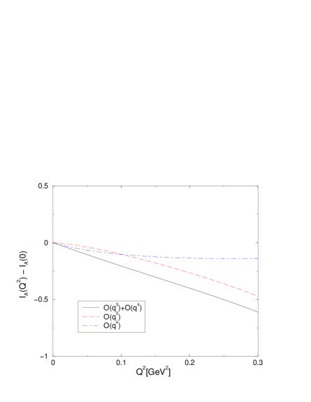
Figure 9: The integrals $I_{A}(Q^{2})-I_{A}(0)$ (left panel) and $I_{C}(Q^{2})-I_{C}(0)$ (right panel) for the neutron in units of GeV^-2. The solid line gives the fourth order result, the third and fourth order contributions are depicted by the dashed and dot–dashed lines, respectively.

Recently, data from Jefferson Lab on the momentum dependence of the generalized DHG sum rule for the neutron at low and intermediate $Q^{2}$ have become available [12]. In Fig. 8 we show the lowest two data points for the integral $I_{A}^{n}(Q^{2})$ in comparison to our theoretical prediction. Consider first the left panel, which refers to the results without the form factor of Eq.(3.14). As stressed before, the theoretical uncertainty is rather large due to the large range of values of delta parameters. It is, however, remarkable that the trend of the data is well described for values of $g_{2},X,Y$ at the upper edge of their allowed values (in magnitude). Positive values for $X,Y$ and the smaller values of $g_{2}$ are clearly excluded from this comparison. For illustration, we show that with the set of parameters $g_{2}=9.5$, $X=Y=-0.725$ one obtains a good description of the data (see the dot–dashed line). In the right panel of that figure, we show the results if in addition the form factor is included. As expected, the allowed band shrinks and furthermore, for the second set of delta parameters the theoretical description turns out to be in rather good agreement with experiment for $Q^{2}\lesssim 0.15$ GeV². The bending of the data to lower values with increasing virtuality cannot be explained any more, which presumably points towards the inadequacy of the form factor Eq.(3.14) for analysing the new precision data. It is also interesting to compare the chiral loop prediction for the integrals $I_{A}(Q^{2})$ and $I_{C}(Q^{2})$, as shown in Fig. 9 for the neutron. While the third and fourth order contributions are rather different, the total one–loop prediction for $I_{A}^{n}(Q^{2})$ and $I_{C}^{n}(Q^{2})$ comes out almost equal, as expected, see Ref. [16].

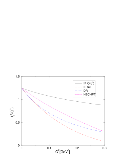
Figure 10: The integral $I_{2}(Q^{2})$ for the proton (left panel) and the neutron (right panel). The solid line gives the complete fourth order result, that is the product of the form factors is taken to that order. Dashed (dot-dashed) line: taking into account the full fourth order (dispersion-theoretical) result for the form factors (i.e. without truncating the product of the form factors). The HBCHPT result of [8] is also shown (dotted line).

We now turn to the BC integrals $I_{2}(Q^{2})$ for the proton and the neutron as shown in Fig. 10. First, we note that the validity of the BC sum rule was shown for HBCHPT in [8], it is also fulfilled if one uses infrared regularization (which is simply a consequence of some general principles like e.g. crossing symmetry). In Fig. 10 we show the result for $I_{2}$ from the IR calculation of [13] where the form factors are taken up to ${\cal O}(q^{4})$ (corresponding to the curve denoted as IR: full). The difference with the dispersion–theoretical result [28] is mostly accounted for by vector mesons and one therefore obtains a rather good description of $I_{2}$ in IR plus vector mesons. However, strictly speaking this does not correspond to an ${\cal O}(q^{4})$ calculation of $I_{2}$, in which one only retains terms in the product of the form factors up-to-and-including fourth order (corresponding to the curve denoted as IR: O($q^{4}$)). It turns out that this ${\cal O}(q^{4})$ calculation is rather far from the empirical results since higher order terms are important. We come back to this issue in Section 4.2. In fact, it turns out that the HBCHPT result of Ref.  [8] looks better though individually the form factors are described slightly worse. However, in that paper the Dirac form factor is simply a constant (that is the charge of the nucleon) and the complete $Q^{2}$–dependence is thus given by the Pauli form factor, quite in contrast to our calculation and the empirical result. Note also that the HBCHPT result shows no curvature in contrast to the empirical curve. Given these observations, we do not share the opinion of the authors of [8] that the BC sum rule is a good observable to bridge the gap between low and high $Q^{2}$.

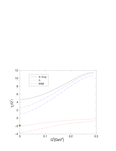
Figure 11: The forward spin polarizability $\gamma_{0}$ at finite virtuality for the proton (left panel) and the neutron (right panel) in units of $10^{-4}$ fm⁴. The solid line gives the fourth order pion loop result, the delta contribution is given by the band spanned by the dashed lines. The total prediction is depicted by the dot–dashed lines. The MAMI data point on $\gamma_{0}^{p}(Q^{2}=0)$ is shown by the circle [14].

In Fig. 11, we show the forward spin polarizability for the proton and the neutron at finite photon virtuality. For the proton, the chiral loop contribution is positive and increasing with increasing $Q^{2}$, while the delta Born graph contribution is negative and essentially flat. In total, the sum is positive, at odds with the measured value of the spin polarizability (at the photon point) [14]. At this point we can only speculate that a combination of higher order and delta loop effects will account for the discrepancy. This deserves further investigation (see also the discussion in Section 4.2). The chiral expansion of $\gamma_{0}^{p}$ will be discussed below. For the neutron, the results are markedly different. While the chiral loop contribution decreases with increasing photon virtuality, the delta Born contribution rises, leading to a slightly decreasing sum. Note also that $\gamma_{0}^{n}$ is negative in contrast to the positive $\gamma_{0}^{p}$, our theoretical bounds are:

$$\phantom{-}1.0\cdot 10^{-4}\,{\rm fm}^{4}\leq\gamma_{0}^{p}\leq\phantom{-}2.6\cdot 10^{-4}\,{\rm fm}^{4}~{},$$ (4.1)

$$-1.8\cdot 10^{-4}\,{\rm fm}^{4}\leq\gamma_{0}^{n}\leq-0.2\cdot 10^{-4}\,{\rm fm}^{4}~{}.$$ (4.2)

One should not be worried about the difference of these numbers to the results presented in [4] because in that paper a third order dimensionally regularized relativistic calculation was performed, which has no consistent underlying power counting. It is interesting to consider the chiral expansion of pion loop contribution to the forward spin polarizability of the proton and the neutron. These can be given in closed analytical form,

$$\gamma_{0}^{p} = {e^{2}g_{A}^{2}\over 96\pi^{3}M_{\pi}^{2}F_{\pi}^{2}}\Biggl{(}1-\biggl{[}{1\over 8}\left(21+3\kappa_{v}+\kappa_{s}\right)\,\pi\,\mu+\biggl{(}\bigl{(}20+{9\over 2}(\kappa_{v}+\kappa_{s})\bigr{)}\,\mu^{2}$$ (4.3)

$$+\,\bigl{(}26+7\kappa_{v}+7\kappa_{s})\,\mu^{2}\ln\mu\biggr{)}-{15\over 64}\bigl{(}125+49\kappa_{v}+63\kappa_{s}\bigr{)}\,\pi\,\mu^{3}\biggr{]}+{\cal O}(\mu^{4})\,\Biggr{)}$$

$$= \underbrace{4.45}_{{\cal O}(\mu^{-2})}-\underbrace{8.31}_{{\cal O}(\mu^{-1})}+\underbrace{6.03}_{{\cal O}(\mu^{0})}+\underbrace{3.22}_{{\cal O}(\mu^{1})}+{\cal O}(\mu^{2})$$

$$= 4.64~{},$$

$$\gamma_{0}^{n} = {e^{2}g_{A}^{2}\over 96\pi^{3}M_{\pi}^{2}F_{\pi}^{2}}\Biggl{(}1-\biggl{[}{1\over 8}\left(9+3\kappa_{v}-\kappa_{s}\right)\,\pi\,\mu+\biggl{(}\bigl{(}5+3\kappa_{v}-3\kappa_{s}\bigr{)}\,\mu^{2}$$ (4.4)

$$+4\,\bigl{(}1+\kappa_{v}-\kappa_{s})\,\mu^{2}\ln\mu\biggr{)}-{15\over 64}\bigl{(}5+15\kappa_{v}-21\kappa_{s}\bigr{)}\,\pi\,\mu^{3}\biggr{]}+{\cal O}(\mu^{4})\,\Biggr{)}$$

$$= \underbrace{4.45}_{{\cal O}(\mu^{-2})}-\underbrace{5.25}_{{\cal O}(\mu^{-1})}+\underbrace{2.00}_{{\cal O}(\mu^{0})}+\underbrace{0.68}_{{\cal O}(\mu^{1})}+{\cal O}(\mu^{2})$$

$$= 1.82~{},$$

where the last number refers to the full (not expanded) result and all numbers are given in the canonical units of $10^{-4}\,$fm⁴. The first term in these series agrees, of course, with the result of [22]. More interesting are, however, the higher order terms which have stirred some controversy within HBCHPT calculations, see [30, 31, 32, 33, 34] (more precisely, this refers to the terms $\sim\mu^{-1}$). Let us consider first the proton. Upon inspection, the chiral expansion does not seem to converge. However, we note that the sum of the four first terms in the expansion is $5.39\cdot 10^{-4}\,$fm⁴, the difference with the full result coming essentially from the ${\cal O}(\mu^{2})$ term, which brings another $-0.64\cdot 10^{-4}\,$fm⁴. Naively, one would expect that the expansion parameter is $\mu\simeq 1/7$, but clearly the appearance of large numerical prefactors, in particular due to the large value of $\kappa_{v}\simeq 3.7$, invalidates such a simple picture. Things look somewhat different for the neutron. The sum of the first four terms amounts to $1.87\cdot 10^{-4}\,$fm⁴, only a few percent off the full result. Note, however, the almost complete cancellation between the first and the second term. Therefore, to make a reliable prediction for the chiral loop contributions to $\gamma_{0}^{n}$, one has to account for the terms of order $\mu$ as done here. To get an idea about the theoretical uncertainty for these numbers, we have replaced the physical values of $\kappa_{v}$ and $\kappa_{s}$ in the above expressions by the values of the LECs $c_{6}$ and $c_{7}$ to third order as given in [13]. To the accuracy we are working, this is legitimate. The resulting values for the forward spin polarizabilities are $\gamma_{0}^{p}=4.95\cdot 10^{-4}\,$fm⁴ and $\gamma_{n}^{0}=1.70\cdot 10^{-4}\,$fm⁴, not very different from the results given above. We have also identified the reason for the bad convergence, it is entirely related to the contributions from the Born terms, as suggested by the method used in [32]. We thus give here the third and fourth order pole and non–pole contributions to $\gamma_{0}^{p,n}$ (note that to third order one has no pole contribution in the case of the neutron):

$$\begin{array}[]{cccccccr}\gamma_{0}^{p,3,{\rm pole}}&=&0&-\,3.12&+\,2.93&+\,1.49&-\,0.29+\dots&=\phantom{-}0.96~{},\\ \gamma_{0}^{p,3,{\rm non-pole}}&=&4.45&-\,2.34&-\,0.02&+\,0.14&+\ldots&=\phantom{-}2.03~{},\\ \gamma_{0}^{p,4,{\rm pole}}&=&0&-\,1.86&+\,2.88&+\,1.91&-\,0.41+\dots&=\phantom{-}2.45~{},\\ \gamma_{0}^{p,4,{\rm non-pole}}&=&0&-\,0.93&+\,0&-\,0.12&+\,0.02+\ldots&=-0.81~{},\\ \end{array}$$ (4.5)

$$\begin{array}[]{cccccccr}\gamma_{0}^{n,3,{\rm non-pole}}&=&4.45&-\,2.34&+\,0.36&+\,0.05&+\ldots&=\phantom{-}2.43~{},\\ \gamma_{0}^{n,4,{\rm pole}}&=&0&-\,1.99&+\,1.74&+\,0.74&-\,0.07+\dots&=\phantom{-}0.42~{},\\ \gamma_{0}^{n,4,{\rm non-pole}}&=&0&-\,0.99&+\,0.24&-\,0.04&-\,0.02+\ldots&=-1.03~{},\\ \end{array}$$ (4.6)

where the first, second, third, $\ldots$ term refers to the terms of order $1/M_{\pi}^{2}$, $1/M_{\pi}$, $M_{\pi}^{0}$, $\ldots$, respectively, and the last one is again the full (unexpanded) result at the given order. All numbers are given in canonical units. One clearly sees that the pole graphs are entirely responsible for the convergence problems, whereas the non–pole terms show a good convergence at third as well as at fourth order. One thus might entertain the possibility of rearranging the power counting accordingly. We come back to this point in Section 4.2. Finally, note that a complete one–loop calculation to ${\cal O}(q^{4})$ within HBCHPT only gives the terms up–to–and–including ${\cal O}(\mu^{-1})$.

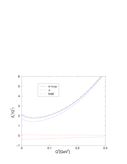
Figure 12: The longitudinal–transverse polarizability $\delta_{0}$ at finite virtuality for the proton (left panel) and the neutron (right panel) in units of $10^{-4}$ fm⁴. The solid line gives the fourth order pion loop result, the delta contribution is given by the band spanned by the dashed lines. The total prediction is depicted by the dot–dashed lines.

In Fig. 12 the longitudinal–transverse spin polarizability for the proton and the neutron at finite virtuality is shown. Here, the delta Born graph contribution is small, as can be easily understood making use of the multipole decomposition of Ref. [16]. Therefore, the chiral prediction for $\delta_{0}^{p,n}(Q^{2})$ is certainly more reliable than for the forward spin polarizabilities. For $\delta_{0}^{n}(Q^{2})$ as well as for $\delta_{0}^{p}(Q^{2})$ the slope at $Q^{2}=0$ is negative, consistent with the HBCHPT result of [8]. At the photon point, we have:

$$1.7\cdot 10^{-4}\,{\rm fm}^{4}\leq\delta_{0}^{p}\leq 2.2\cdot 10^{-4}\,{\rm fm}^{4}~{},$$ (4.7)

$$2.3\cdot 10^{-4}\,{\rm fm}^{4}\leq\delta_{0}^{n}\leq 2.8\cdot 10^{-4}\,{\rm fm}^{4}~{}.$$ (4.8)

We note that these numbers are not very different from the leading $1/M_{\pi}^{2}$ singularity, which gives $\delta_{0}^{p}=\delta_{0}^{n}=2.23\cdot 10^{-4}\,$fm⁴. This can be made more transparent by considering the chiral expansion of these quantities. We find

$$\delta_{0}^{p} = {e^{2}g_{A}^{2}\over 192\pi^{3}M_{\pi}^{2}F_{\pi}^{2}}\Biggl{(}1+\biggl{[}{1\over 8}\bigl{(}-9+\kappa_{v}+4\kappa_{s}\bigr{)}\,\pi\,\mu+\biggl{(}\biggl{(}-3+\frac{3}{16}(15\kappa_{v}+11\kappa_{s})\biggr{)}\,\mu^{2}$$ (4.9)

$$+\,\frac{3}{8}\biggl{(}-\kappa_{v}+11\kappa_{s}\biggr{)}\,\mu^{2}\ln\mu\biggr{)}-{3\over 64}\biggl{(}119-15(4\kappa_{v}-5\kappa_{s})\biggr{)}\,\pi\,\mu^{3}\biggr{]}+{\cal O}(\mu^{4})\,\Biggr{)}$$

$$= \underbrace{2.23}_{{\cal O}(\mu^{-2})}-\underbrace{0.75}_{{\cal O}(\mu^{-1})}+\underbrace{0.53}_{{\cal O}(\mu^{0})}+\underbrace{0.12}_{{\cal O}(\mu^{1})}+{\cal O}(\mu^{2})$$

$$= 2.04~{},$$

$$\delta_{0}^{n} = {e^{2}g_{A}^{2}\over 192\pi^{3}M_{\pi}^{2}F_{\pi}^{2}}\Biggl{(}1+\biggl{[}{1\over 8}\bigl{(}3+\kappa_{v}-4\kappa_{s}\bigr{)}\,\pi\,\mu+\biggl{(}\biggl{(}7+3\kappa_{v}-\frac{3}{2}\kappa_{s}\biggr{)}\,\mu^{2}$$ (4.10)

$$+\,12\biggl{(}1-\frac{1}{4}\kappa_{s}\biggr{)}\,\mu^{2}\ln\mu\biggr{)}-{3\over 64}\biggl{(}275-15(\kappa_{v}+4\kappa_{s})\biggr{)}\,\pi\,\mu^{3}\biggr{]}+{\cal O}(\mu^{4})\,\Biggr{)}$$

$$= \underbrace{2.23}_{{\cal O}(\mu^{-2})}+\underbrace{0.93}_{{\cal O}(\mu^{-1})}-\underbrace{0.26}_{{\cal O}(\mu^{0})}-\underbrace{0.24}_{{\cal O}(\mu^{1})}+{\cal O}(\mu^{2})$$

$$= 2.66~{},$$

where again the number in the last row refers to the full one–loop result and all numbers are given in units of $10^{-4}\,{\rm fm}^{4}$. The chiral expansion of $\delta_{0}^{p}$ is very well behaved, furthermore, the sum of the first four terms in the series is $2.13\cdot 10^{-4}\,{\rm fm}^{4}$, only 4% off the full result. For the neutron, we observe that the sum of the first four terms, which is $2.66\cdot 10^{-4}\,{\rm fm}^{4}$, essentially amounts to the total sum at one loop. The chiral expansion of $\delta_{0}^{n}$ is well behaved, although the terms of order $\mu^{0}$ are somewhat small. We note that in contrast to the chiral expansion of $\gamma_{0}^{p,n}$ no unnaturally large prefactors appear here. It thus appears that the longitudinal–transverse spin polarizability is a better suited observable to test the chiral dynamics of QCD. Finally, we have also calculated the longitudinal–transverse spin polarizabilities using the third order values for $c_{6,7}$ instead of the physical values for $\kappa_{s,v}$. This results in $\delta_{0}^{p}=2.45\cdot 10^{-4}\,{\rm fm}^{4}$ and $\delta_{0}^{n}=3.13\cdot 10^{-4}\,{\rm fm}^{4}$.

4.2 Beyond fourth order

As we have seen e.g. in the discussion of the forward spin polarizabilities, the calculation of the Born graphs to fourth order is not quite sufficient in some cases to obtain convergence. This observation was also behind the modified method to obtain the spin polarizabilities from the spin–structure amplitudes used in [32]. We therefore assume that the missing physics largely resides in these Born terms, more specifically in the leading two–loop corrections that appear at fifth order. While a complete fifth order calculation goes beyond the scope of this paper, it is straightforward to calculate the contribution from the pole diagrams shown in Fig. 13 (for the combination of structure functions $S_{1}(\nu,Q^{2})-(Q^{2}/m\nu)\,S_{2}(\nu,Q^{2}))$. This class of diagrams is gauge–invariant and, of course, does not modify any LET or the DHG and BC sum rules. However, new LECs related to dimension two insertions as in diagram 5t and dimension four insertions as in diagram 5u appear. These have, however, already been determined in the analysis of pion–nucleon scattering [36] and of the nucleons’ electromagnetic form factors [13]. We use the same values, i.e. $c_{4}=3.4\,$GeV^-1, $e_{54}=0.26\,$GeV^-3 and $e_{74}=1.65\,$GeV^-3 . Other operators that appear in the chiral expansion of the nucleon from factors [13] do not contribute to the particular combination of the structure functions we are considering here. Note that here we concentrate on the neutron, simply because there are much less diagrams to calculate than in the case of the proton due to the non–vanishing charge (dimension one insertion). For further calculational simplicity, we restrict these considerations to observables that can be derived from the combination of structure functions $S_{1}(\nu,Q^{2})-(Q^{2}/m\nu)\,S_{2}(\nu,Q^{2})$. Of course, one should devise a modified power counting to properly account for these effects. A resummation of these terms also to higher order could be obtained by including the pertinent higher order insertions in the baryon propagator. Whether this can be done in a systematic fashion consistent with already existing successful calculations of other observables remains to be seen. Here, we are only interested to investigate whether these terms indeed contribute significantly in the problematic cases, these are the forward spin polarizability and the convergence of the BC sum rule.

Consider first the BC sum rule for the neutron. Here, we have performed the complete fifth order calculation since only Born terms contribute. As shown in Fig. 14, there are sizeable corrections when going from fourth to fifth order in the expansion of the product of the form factors. On the other hand, for $Q^{2}\lesssim 0.15\,$GeV², the fifth order result is not very different from the “full fourth order” result (meaning that the form factors are taken to fourth order, not their product). Finally, we turn to the forward spin polarizability of the neutron. Using the same notation as in Eq.(4.6), we find (in canonical units):

$$\begin{array}[]{cccccccccr}\gamma_{0}^{n,5,{\rm pole}}&=&0&+\,0&+\,0.02&-\,1.36&-\,0.18&-\,0.09&+\dots&=-1.41~{},\\ \end{array}$$ (4.11)

where the first two zeros are consistent with the power counting, i.e. that the two leading chiral singularities $\sim 1/M_{\pi}^{2}$ and $\sim 1/M_{\pi}$ are not affected at two (and higher) loop accuracy. Thus, the Born contribution gets sizeably reduced at this order. It is also interesting to note that the formally leading term $\sim\mu^{0}$ is very small. Since the proton pole contributions have the same sign as the ones from the neutron and are larger in magnitude (related largely to the fact that the magnetic moment is larger), one can speculate that these terms will sizeably reduce the positive prediction, cf. Eq.(4.1). Such a calculation should be done but goes beyond the scope of this article. Finally, we have considered the moment $I_{A}^{n}(Q^{2})$. Although we find some sizeable fifth order corrections from the Born terms, these are counterbalanced to a large extent by vector meson contributions, so that the ensuing band for the theoretical prediction is not very far from the fourth order one as given in Fig. 8

Appendix A Chiral contributions to the structure functions

Here, we give the explicit expressions for the reduced invariant functions $A(s,Q^{2})$ and $B(s,Q^{2})$ as defined in Eq.(2.1), for the third and fourth order contributions. Throughout, the contribution from the elastic intermediate state is subtracted. For notational simplicity, we do not display the bar as done for the structure functions $S_{1,2}^{p,n}(\nu,Q^{2})$ in the main text, cf. Eq. (2.6). Note that the $B(s,Q^{2})$ as given below correspond to the quantity

$$\nu\bar{\underline{S}}_{2}(\nu,Q^{2})=\nu\bar{S}_{2}(\nu,Q^{2})-\nu\bar{S}_{2}(\nu,Q^{2})\big{|}_{\nu=0}\,,$$

that is they allow to calculate the moments of $\bar{S}_{2}$ for $i\geq 1$. However, from the ${\cal O}(q^{4})$ graphs which have an elastic piece, i.e 4(a)-4(j), one gets an additional inelastic contribution. Indeed, one has:

$$B(s,Q^{2})-B(2m^{2}-2Q^{2}-s,Q^{2})=e^{2}\frac{\nu}{\nu^{2}-\nu_{B}^{2}}{\tilde{B}}(Q^{2})+\ldots~{},$$ (A.1)

where $\nu_{B}=Q^{2}/2m$ and the ellipsis denotes the inelastic contribution given below. Using the fact that the pole contribution to $\nu S_{2}$ reads

$$\nu S_{2}(\nu,Q^{2})^{\rm pole}=\frac{e^{2}}{2}\frac{\nu_{B}^{2}}{\nu^{2}-\nu_{B}^{2}}F_{2}(Q^{2})(F_{1}(Q^{2})+F_{2}(Q^{2}))$$ (A.2)

one gets:

$$S_{2}^{(-1)}(0,Q^{2})={\tilde{B}}(Q^{2})=\frac{1}{2}F_{2}(Q^{2})(F_{1}(Q^{2})+F_{2}(Q^{2}))$$ (A.3)

It is straightforward to check that this relation holds.

Consider first the third order diagrams given in Fig. 1 and their crossed partners. We have (whenever appropriate, we add together the contributions from various diagrams):

3a

$$A(s,Q^{2}) = {me^{2}g_{A}^{2}\over 2F^{2}}\,\Bigl{[}J_{0}(s)+{1\over 2m^{2}}(s+m^{2}+Q^{2})J_{1}(s)\Bigr{]}~{},$$

$$B(s,Q^{2}) = 0~{}.$$ (A.4)

3b+3c

$$A(s,Q^{2}) = {me^{2}g_{A}^{2}\over F^{2}}\,\Bigl{[}J_{0}(s)-{1\over 2m^{2}}(s+m^{2}+Q^{2})J_{1}(s)-2Q^{2}\Gamma_{1}(s,Q^{2})$$

$$+(s-m^{2}+Q^{2})\Gamma_{2}(s,Q^{2})+4\Gamma_{3}(s,Q^{2})\Bigr{]}\,\frac{1}{2}(1-\tau_{3})~{},$$

$$B(s,Q^{2}) = {2me^{2}g_{A}^{2}\over F^{2}}\,\Bigl{[}\Gamma_{1}(s,Q^{2})-\Gamma_{4}(s,Q^{2})\Bigr{]}\,\frac{1}{2}(1-\tau_{3})~{}.$$ (A.5)

3d+3e

$$A(s,Q^{2}) = {4me^{2}g_{A}^{2}\over F^{2}}\,\gamma_{3}(s,Q^{2})~{},$$

$$B(s,Q^{2}) = -{me^{2}g_{A}^{2}\over F^{2}}\,\Bigl{[}2\gamma_{4}(s,Q^{2})+\gamma_{1}(s,Q^{2})\Bigr{]}~{}.$$ (A.6)

3f

$$A(s,Q^{2}) = {4me^{2}g_{A}^{2}\over F^{2}}\,\Bigl{[}-\gamma_{3}(s,Q^{2})+{1\over 2}(s-m^{2}+Q^{2})\Omega_{3}(s,Q^{2})\Bigr{]}\,\frac{1}{2}(1-\tau_{3})~{},$$

$$B(s,Q^{2}) = {me^{2}g_{A}^{2}\over F^{2}}\,\Bigl{[}2\gamma_{4}(s,Q^{2})+\gamma_{1}(s,Q^{2})+2m^{2}\Omega_{5}(s,Q^{2})\Bigr{]}\,\frac{1}{2}(1-\tau_{3})~{}.$$ (A.7)

3g

$$A(s,Q^{2}) = {me^{2}g_{A}^{2}\over F^{2}}\,\Bigl{[}-\frac{3}{2}J_{0}(s)+{1\over 4m^{2}}(s+m^{2}+Q^{2})J_{1}(s)+(s-m^{2}+3Q^{2})\Gamma_{1}(s,Q^{2})$$

$$+(3m^{2}-Q^{2}-s)\Gamma_{2}(s,Q^{2})-4\Gamma_{3}(s,Q^{2})+(6-d)(s-m^{2}+Q^{2})G_{3}(s,Q^{2})$$

$$-Q^{2}(s-m^{2}+Q^{2})G_{4}(s,Q^{2})-4m^{2}Q^{2}G_{5}(s,Q^{2})+m^{2}(s-m^{2}+Q^{2})G_{6}(s,Q^{2})\Bigr{]}\,\frac{1}{4}(3-\tau_{3})~{},$$

$$B(s,Q^{2}) = -{2me^{2}g_{A}^{2}\over F^{2}}\,\Bigl{[}\Gamma_{1}(s,Q^{2})-\Gamma_{4}(s,Q^{2})\Bigr{]}\,\frac{1}{4}(3-\tau_{3})~{}.$$ (A.8)

3h

$$A(s,Q^{2}) = {me^{2}g_{A}^{2}\over F^{2}}\,\Bigl{[}-\frac{3}{4}J_{0}(s)+{3\over 8m^{2}}(s+m^{2}+Q^{2})J_{1}(s)-\frac{3Q^{2}}{2(s-m^{2})}\Bigl{(}\underline{J}_{0}(s)-2\underline{J}_{1}(s)\Bigr{)}$$ (A.9)

$$-\frac{3Q^{2}m^{2}}{(s-m^{2})^{2}}\Bigl{(}\underline{\underline{J}}_{0}(s)-\underline{\underline{J}}_{1}(s)\Bigr{)}\Bigr{]}\,\frac{1}{2}(1+\tau_{3})~{},$$

3i+3j

$$A(s,Q^{2}) = {me^{2}g_{A}^{2}\over F^{2}}\,\Bigl{[}\frac{1}{2m^{2}}(m^{2}-Q^{2}-s)J_{1}(s)-\frac{Q^{2}}{s-m^{2}}\Bigl{(}\underline{J}_{1}(s)-\underline{J}_{0}(s)\Bigr{)}\Bigr{]}\,\frac{1}{2}(1+\tau_{3})~{},$$ (A.10)

3k+3l

$$A(s,Q^{2}) = {me^{2}g_{A}^{2}\over F^{2}}\,\Bigl{(}\frac{4Q^{2}}{s-m^{2}}\Bigr{)}\,\underline{\gamma}_{3}(s,Q^{2})\,\frac{1}{2}(1+\tau_{3})~{},$$ (A.11)

3m+3n

$$A(s,Q^{2}) = {me^{2}g_{A}^{2}\over F^{2}}\,\Bigl{[}\frac{1}{4m^{2}}(m^{2}-Q^{2}-s)J_{1}(s)-Q^{2}\Gamma_{1}(s,Q^{2})+\frac{1}{2}(s-m^{2}+Q^{2})\Gamma_{2}(s,Q^{2})+Q^{2}\Gamma_{5}(s,Q^{2})$$ (A.12)

$$\qquad\qquad-\frac{Q^{2}}{s-m^{2}}\Bigl{(}\frac{1}{2}\underline{J}_{1}(s)-\frac{1}{2}\underline{J}_{0}(s)-(d-2)\underline{\Gamma}_{3}(s,Q^{2})+Q^{2}\underline{\Gamma}_{4}(s,Q^{2})$$

$$\qquad\qquad\qquad-Q^{2}\underline{\Gamma}_{5}(s,Q^{2})-m^{2}\underline{\Gamma}_{6}(s,Q^{2})\Bigr{)}\Bigr{]}\,\frac{1}{2}(1+\tau_{3})~{}.$$

3h+3i+3j+3k+3l+3m+3n

$$B(s,Q^{2}) = {me^{2}g_{A}^{2}\over F^{2}}\,\Bigl{[}\gamma_{1}(s,Q^{2})+2\gamma_{4}(s,Q^{2})+\frac{2m^{2}}{s-m^{2}}\Bigl{(}\underline{\gamma}_{2}(s,Q^{2})+2\underline{\gamma}_{5}(s,Q^{2})\Bigr{)}\Bigr{]}\,\frac{1}{2}(1+\tau_{3})~{},$$ (A.13)

with

$$\underline{F}(s,Q^{2}) = F(s,Q^{2})-F(m^{2},Q^{2})~{},$$

$$\underline{\underline{F}}(s,Q^{2}) = \underline{F}(s,Q^{2})-(s-m^{2})\underline{F}^{\prime}(m^{2},Q^{2})~{},$$ (A.14)

where the prime denotes differentiation with respect to $s$ with $s=(p+q)^{2}=2m\nu+m^{2}-Q^{2}$ the standard Mandelstam variable and $\nu$ is the energy transfer. The various loop functions are generalizations of the ones defined for $Q^{2}=0$ in Ref. [15] to virtual photons with $Q^{2}>0$ using

$$h_{\gamma}(x,y;s,Q^{2})=M_{\pi}^{2}(1-y)+M^{2}y^{2}+(s-M^{2})xy(y-1)+Q^{2}x(1-x)(1-y)^{2}$$ (A.15)

in their Feynman parameter representation. Note that the result for $A(s,Q^{2})$ agrees (up to an overall factor of $m$) with the relativistic one given in Appendix A of Ref. [4] if one uses the relations

$$(s-m^{2}+Q^{2})\Omega_{3}(s,Q^{2}) = \gamma_{3}(s,Q^{2})+\Gamma_{3}(s,Q^{2})-(s\to 2m^{2}-2Q^{2}-s)~{},$$

$$2G_{3}(s,Q^{2}) = \Gamma_{4}(s,Q^{2})-\Gamma_{2}(s,Q^{2})~{},$$ (A.16)

that hold in dimensionally regularized but not in infrared regularized baryon CHPT.

Consider now the fourth order diagrams given in Fig. 2 and their crossed partners. After properly taking into account the renormalization of the anomalous magnetic moment [13], we find (whenever appropriate, we add together the contributions from various diagrams. In particular, we have not shown the diagrams which arise from a trivial reordering of the two vertices, like e.g. for the contribution from graphs 4e)+4f). Such contributions are included in the results given.):

4a+4b+4c+4d

$$A^{n}(s,Q^{2}) = {e^{2}g_{A}^{2}\over 4mF^{2}}\,{1\over 2}\,(\kappa_{s}-\kappa_{v})\Bigl{\{}-2(s-m^{2}+Q^{2})\Bigl{[}(s-m^{2})(\Gamma_{1}(s,Q^{2})-\Gamma_{5}(s,Q^{2}))+(2-d)\Gamma_{3}(s,Q^{2})$$

$$+Q^{2}(\Gamma_{4}(s,Q^{2})-\Gamma_{5}(s,Q^{2}))-m^{2}\Gamma_{6}(s,Q^{2})+2\gamma_{3}(s,Q^{2})\Bigr{]}-4m^{2}Q^{2}(2\Gamma_{1}(s,Q^{2})-\Gamma_{2}(s,Q^{2})$$

$$-2\Gamma_{5}(s,Q^{2}))-\frac{8Q^{2}m^{2}}{s-m^{2}}\Bigl{[}(2-d)\underline{\Gamma}_{3}(s,Q^{2})+Q^{2}(\underline{\Gamma}_{4}(s,Q^{2})-\underline{\Gamma}_{5}(s,Q^{2}))$$

$$-m^{2}\underline{\Gamma}_{6}(s,Q^{2})+2\gamma_{3}(s,Q^{2})\Bigr{]}\Bigl{\}}$$

$$B^{n}(s,Q^{2}) = {e^{2}g_{A}^{2}\over 4mF^{2}}\,{1\over 2}\,(\kappa_{s}-\kappa_{v})\Bigl{\{}2m^{2}\Bigl{[}6\Gamma_{1}(s,Q^{2})-\Gamma_{2}(s,Q^{2})-4\Gamma_{4}(s,Q^{2})-4\Gamma_{5}(s,Q^{2})-2\gamma_{1}(s,Q^{2})$$

$$-\gamma_{2}(s,Q^{2})-4\gamma_{4}(s,Q^{2})-2\gamma_{5}(s,Q^{2})\Bigr{]}+2J_{21}^{\pi\pi}(Q^{2})-3J_{1}^{\pi\pi}(Q^{2})+J_{\pi\pi}(Q^{2})$$

$$+\frac{2m^{2}}{s-m^{2}}\Bigl{[}2(2-d)\underline{\Gamma}_{3}(s,Q^{2})+2Q^{2}\underline{\Gamma}_{4}(s,Q^{2})-2(4m^{2}+Q^{2})\underline{\Gamma}_{5}(s,Q^{2})-2m^{2}\underline{\Gamma}_{6}(s,Q^{2})$$

$$+4\underline{\gamma}_{3}(s,Q^{2})-4m^{2}(\underline{\gamma}_{2}(s,Q^{2})+2\underline{\gamma}_{5}(s,Q^{2}))\Bigr{]}\Bigl{\}}~{},$$

$$A^{p}(s,Q^{2}) = {e^{2}g_{A}^{2}\over 4mF^{2}}\,{1\over 2}\,(\kappa_{s}+\kappa_{v})\Bigl{\{}-(s-m^{2}+Q^{2})\Bigl{[}-\frac{3}{2}(J^{\pi N}(s)-J_{1}^{\pi N}(s))+(s-m^{2})\Gamma_{1}(s,Q^{2})$$

$$+(2-d)\Gamma_{3}(s,Q^{2})+Q^{2}\Gamma_{4}(s,Q^{2})+(m^{2}-Q^{2}-s)\Gamma_{5}(s,Q^{2})-m^{2}\Gamma_{6}(s,Q^{2})-4\gamma_{3}(s,Q^{2})\Bigr{]}$$

$$-3Q^{2}J_{1}^{\pi N}(s)-2m^{2}Q^{2}(2\Gamma_{1}(s,Q^{2})-\Gamma_{2}(s,Q^{2})-2\Gamma_{5}(s,Q^{2}))$$

$$-\frac{4Q^{2}m^{2}}{s-m^{2}}\Bigl{[}-\frac{3}{2}(\underline{J}^{\pi N}(s)-\underline{J}_{1}^{\pi N}(s))+(2-d)\underline{\Gamma}_{3}(s,Q^{2})+Q^{2}(\underline{\Gamma}_{4}(s,Q^{2})-\underline{\Gamma}_{5}(s,Q^{2}))$$

$$\qquad\qquad\qquad-m^{2}\underline{\Gamma}_{6}(s,Q^{2})-4\gamma_{3}(s,Q^{2})\Bigr{]}\Bigl{\}}$$

$$B^{p}(s,Q^{2}) = -{e^{2}g_{A}^{2}\over 4mF^{2}}\,{1\over 2}\,(\kappa_{s}+\kappa_{v})\Bigl{\{}2m^{2}\Bigl{[}3\Gamma_{1}(s,Q^{2})-\frac{1}{2}\Gamma_{2}(s,Q^{2})-2\Gamma_{4}(s,Q^{2}))-2\Gamma_{5}(s,Q^{2})+2\gamma_{1}(s,Q^{2})$$ (A.17)

$$+4\gamma_{4}(s,Q^{2})\Bigr{]}+\frac{3}{2}J_{1}^{\pi N}(s)-2J_{21}^{\pi\pi}(Q^{2})+3J_{1}^{\pi\pi}(Q^{2})-J_{\pi\pi}(Q^{2})+\frac{2m^{2}}{s-m^{2}}\Bigl{[}-\frac{3}{2}(\underline{J}^{\pi N}(s)-\underline{J}_{1}^{\pi N}(s))$$

$$+(2-d)\underline{\Gamma}_{3}(s,Q^{2})-Q^{2}(\underline{\Gamma}_{5}(s,Q^{2})-\underline{\Gamma}_{4}(s,Q^{2}))-m^{2}(\underline{\Gamma}_{6}(s,Q^{2})+4\underline{\Gamma}_{5}(s,Q^{2}))$$

$$\qquad\qquad+4m^{2}(\underline{\gamma}_{2}(s,Q^{2})+2\underline{\gamma}_{5}(s,Q^{2}))-4\underline{\gamma}_{3}(s,Q^{2})\Bigr{]}\Bigl{\}}~{}.$$

4g

$$A^{p}(s,Q^{2}) = {e^{2}g_{A}^{2}\over 4mF^{2}}\,\Bigl{(}-{3\over 4}\Bigr{)}\,(\kappa_{s}+\kappa_{v})\Bigl{[}-\frac{16m^{4}Q^{2}}{(s-m^{2})^{2}}\Bigl{(}\underline{\underline{J}}_{1}(s)-\underline{\underline{J}}_{0}(s)\Bigr{)}-\frac{4m^{2}Q^{2}}{s-m^{2}}\Bigl{(}\underline{\underline{J}}_{1}(s)-\underline{\underline{J}}_{0}(s)+4\underline{J}_{1}(s)-2\underline{J}_{0}\Bigr{)}$$

$$-4m^{2}(\underline{\underline{J}}_{1}(s)-\underline{\underline{J}}_{0}(s))-(s-m^{2}+Q^{2})(3\underline{J}_{1}(s)-\underline{J}_{0}(s))-2Q^{2}J_{1}(s)\Bigr{]}~{},$$

$$B^{p}(s,Q^{2}) = {e^{2}g_{A}^{2}\over 4mF^{2}}\,{3\over 4}\,(\kappa_{s}+\kappa_{v})\Bigl{[}\frac{8m^{4}}{(s-m^{2})^{2}}\Bigl{(}\underline{\underline{J}}_{1}(s)-\underline{\underline{J}}_{0}(s)\Bigr{)}+\frac{4m^{2}}{s-m^{2}}\Bigl{(}2\underline{J}_{1}(s)-\underline{J}_{0}(s)\Bigr{)}+J_{1}(s)\Bigr{]}~{}.$$ (A.18)

4j

$$A(s,Q^{2}) = {e^{2}g_{A}^{2}\over 4mF^{2}}\,{1\over 4}\,(1+\tau_{3})\,(3\kappa_{s}-\kappa_{v})\Bigl{\{}-(s-m^{2}+Q^{2})\Bigl{[}J_{1}(s)-J_{0}(s)+2(s-m^{2}+Q^{2})\Gamma_{2}(s,Q^{2})$$

$$\qquad-2M_{\pi}^{2}\Gamma_{0}(s,Q^{2})+4\Gamma_{3}(s,Q^{2})\Bigr{]}+2Q^{2}\Bigl{(}J_{1}(s)-4m^{2}\Gamma_{1}(s,Q^{2})\Bigr{)}$$

$$\qquad\qquad-{8Q^{2}m^{2}\over s-m^{2}}\Bigl{(}2\underline{\Gamma}_{3}(s,Q^{2})-M_{\pi}^{2}\underline{\Gamma}_{0}(s,Q^{2})\Bigr{)}\Bigr{\}}$$

$$B(s,Q^{2}) = {e^{2}g_{A}^{2}\over 8mF^{2}}\,{1\over 4}\,(1+\tau_{3})\,(3\kappa_{s}-\kappa_{v})\Bigl{\{}J_{1}(s)-2m^{2}(\Gamma_{2}(s,Q^{2})+2\Gamma_{5}(s,Q^{2}))$$

$$+{4m^{2}\over s-m^{2}}\Bigl{[}\frac{1}{4}\Bigl{(}J_{1}(s)-J_{0}(s))+M_{\pi}^{2}\Gamma_{0}(s,Q^{2})-4\Gamma_{3}(s,Q^{2})+2Q^{2}(\underline{\Gamma}_{4}(s,Q^{2})-\underline{\Gamma}_{5}(s,Q^{2}))\Bigr{]}\Bigr{\}}~{}.$$

4k+4l

$$A(s,Q^{2}) = {e^{2}g_{A}^{2}\over 4mF^{2}}\,{1\over 2}\,(-\kappa_{v}+\kappa_{s}\tau_{3})\Bigl{\{}(s-m^{2}+Q^{2})\Bigl{[}J_{0}(s)+J_{1}(s)-2M_{\pi}^{2}\Gamma_{0}(s,Q^{2})+2Q^{2}\Gamma_{1}(s,Q^{2})$$

$$-4m^{2}\Gamma_{2}(s,Q^{2})+8\Gamma_{3}(s,Q^{2})-4Q^{2}\Gamma_{4}(s,Q^{2})+2(s-m^{2}+Q^{2})\Gamma_{5}(s,Q^{2})+4m^{2}\Gamma_{6}(s,Q^{2})\Bigr{]}$$

$$-2Q^{2}\Bigl{(}J_{1}(s)-2m^{2}\Bigl{(}2\Gamma_{1}(s,Q^{2})+\Gamma_{2}(s,Q^{2})-2\Gamma_{5}(s,Q^{2})\Bigr{)}\Bigr{)}\Bigr{\}}$$

$$B(s,Q^{2}) = -{e^{2}g_{A}^{2}\over 4mF^{2}}\,{1\over 2}\,\,(-\kappa_{v}+\kappa_{s}\tau_{3})\Bigl{[}J_{1}(s)-2m^{2}\Bigl{(}2\Gamma_{1}(s,Q^{2})+\Gamma_{2}(s,Q^{2})-2\Gamma_{5}(s,Q^{2})\Bigl{)}\Bigr{]}~{}.$$ (A.20)

4m

$$A(s,Q^{2}) = {e^{2}g_{A}^{2}\over 4mF^{2}}\,{1\over 2}\,(-\kappa_{v}+\kappa_{s}\tau_{3})\Bigl{[}4(s-m^{2}+Q^{2})\gamma_{3}(s,Q^{2})-16m^{2}\Gamma_{3}(s,Q^{2})\Bigr{]}~{},$$

$$B(s,Q^{2}) = {e^{2}g_{A}^{2}\over 4mF^{2}}\,{1\over 2}\,\,(-\kappa_{v}+\kappa_{s}\tau_{3})4m^{2}\,\Bigl{[}\Gamma_{1}(s,Q^{2})-2\Gamma_{4}(s,Q^{2})-{1\over 2}\gamma_{2}(s,Q^{2})-\gamma_{5}(s,Q^{2})+M_{\pi}^{2}\Omega_{1}(s,Q^{2})\Bigr{]}~{}.$$

4n+4o

$$A(s,Q^{2}) = {e^{2}g_{A}^{2}\over 4mF^{2}}\,{1\over 4}\,(3-\tau_{3})\,(\kappa_{s}+\kappa_{v})\Bigl{\{}(s-m^{2}+Q^{2})\Bigl{[}{1\over 2}\Bigl{(}J_{0}(s)+J_{1}(s)\Bigr{)}-(s-m^{2}-Q^{2})\Gamma_{1}(s,Q^{2})$$

$$-2m^{2}\Gamma_{2}(s,Q^{2})+2\Gamma_{3}(s,Q^{2})-2Q^{2}\Gamma_{4}(s,Q^{2})+(s-m^{2}+Q^{2})\Gamma_{5}(s,Q^{2})+2m^{2}\Gamma_{6}(s,Q^{2})$$

$$+8m^{2}G_{3}(s,Q^{2})\Bigr{]}-Q^{2}\Bigl{(}J_{1}(s)-4m^{2}(\Gamma_{2}(s,Q^{2})-\Gamma_{5}(s,Q^{2})-M_{\pi}^{2}G_{0}(s,Q^{2})+2G_{3}(s,Q^{2}))\Bigr{)}$$

$$\qquad\qquad\qquad-8m^{2}(\Gamma_{3}(s,Q^{2})-\Gamma_{3}(M^{2},Q^{2}))\Bigr{\}}~{},$$

$$B(s,Q^{2}) = {e^{2}g_{A}^{2}\over 4mF^{2}}\,{1\over 2}\,(3-\tau_{3})\,(\kappa_{s}+\kappa_{v})\,\Bigl{\{}-\frac{1}{4}J_{1}(s)+m^{2}\Bigl{[}\Gamma_{2}(s,Q^{2})-2\Gamma_{4}(s,Q^{2})-M_{\pi}^{2}(G_{0}(s,Q^{2})$$ (A.22)

$$+2G_{1}(s,Q^{2}))+4G_{3}(s,Q^{2})-(m^{2}-Q^{2}-s)(2G_{4}(s,Q^{2})-G_{5}(s,Q^{2}))\Bigr{]}\Bigr{\}}~{}.$$

Figures

Figure 1: Feynman diagrams contributing at third order. Solid, dashed and wiggly lines denote nucleons, pions and photons, in order. All insertions are from the leading order (dimension one) effective Lagrangian. Crossed diagrams are not shown.

Figure 2: Topologically inequivalent Feynman diagrams contributing at fourth order. Solid, dashed and wiggly lines denote nucleons, pions and photons, in order. The black filled circle denotes an insertion from the dimension two effective Lagrangian. All other insertions are from the leading order (dimension one) effective Lagrangian. Crossed diagrams are not shown.

 

Figure 13: Topologically different pole diagrams for V²CS off the neutron contributing at fifth order to the combination of structure functions $S_{1}(\nu,Q^{2})-(Q^{2}/m\nu)\,S_{2}(\nu,Q^{2})$. Solid, dashed and wiggly lines denote nucleons, pions and photons, in order. The black filled circle (square) denotes an insertion from the dimension two (four) effective Lagrangian. All other insertions are from the leading order (dimension one) effective Lagrangian. Crossed diagrams are not shown.

References

- [1] B. W. Filippone and X. D. Ji, Adv. Nucl. Phys. 26 (2002) 1 [arXiv:hep-ph/0101224].
- [2] V. Bernard, N. Kaiser and U.-G. Meißner, Int. J. Mod. Phys. E 4 (1995) 193 [arXiv:hep-ph/9501384].
- [3] V. Bernard, N. Kaiser and U.-G. Meißner, Phys. Rev. D 48 (1993) 3062 [arXiv:hep-ph/9212257].
- [4] J. Edelmann, N. Kaiser, G. Piller and W. Weise, Nucl. Phys. A 641 (1998) 119 [arXiv:nucl-th/9806096].
- [5] X. D. Ji, C. W. Kao and J. Osborne, Phys. Lett. B 472 (2000) 1 [arXiv:hep-ph/9910256].
- [6] X. D. Ji and J. Osborne, J. Phys. G 27 (2001) 127 [arXiv:hep-ph/9905410].
- [7] V. D. Burkert, Phys. Rev. D 63 (2001) 097904 [arXiv:nucl-th/0004001].
- [8] C. W. Kao, T. Spitzenberg and M. Vanderhaeghen, arXiv:hep-ph/0209241.
- [9] V. Bernard, T. R. Hemmert and U.-G. Meißner, Phys. Lett. B 545 (2002) 105 [arXiv:hep-ph/0203167].
- [10] T. Becher and H. Leutwyler, Eur. Phys. J. C 9 (1999) 643 [arXiv:hep-ph/9901384].
- [11] V. Burkert, arXiv:hep-ph/0211185.
- [12] M. Amarian et al. [The Jefferson Lab E94010 Collaboration], Phys. Rev. Lett. 89 (2002) 242301 [arXiv:nucl-ex/0205020].
- [13] B. Kubis and Ulf-G. Meißner, Nucl. Phys. A 679 (2001) 698. [arXiv:hep-ph/0007056].
- [14] J. Ahrens et al. [GDH Collaboration], Phys. Rev. Lett. 87 (2001) 022003 [arXiv:hep-ex/0105089].
- [15] V. Bernard, N. Kaiser and U.-G. Meißner, Nucl. Phys. B 373 (1992) 346.
- [16] D. Drechsel, S. S. Kamalov and L. Tiator, Phys. Rev. D 63 (2001) 114010 [arXiv:hep-ph/0008306].
- [17] F. E. Low, Phys. Rev. 96 (1954) 1428; M. Gell-Mann and M. L. Goldberger, Phys. Rev. 96 (1954) 1433.
- [18] S. B. Gerasimov, Yad. Fiz. 2 (1965) 598 [Sov. J. Nucl. Phys. 2 (1966) 430]; S. D. Drell and A. C. Hearn, Phys. Rev. Lett. 16 (1966) 908.
- [19] K. Helbing [GDH Collaboration], Nucl. Phys. Proc. Suppl. 105 (2002) 113.
- [20] M. Anselmino, B. L. Ioffe and E. Leader, Sov. J. Nucl. Phys. 49 (1989) 136 [Yad. Fiz. 49 (1989) 214].
- [21] H. Burkhardt and W. N. Cottingham, Annals Phys. 56 (1970) 453.
- [22] V. Bernard, N. Kaiser, J. Kambor and U.-G. Meißner, Nucl. Phys. B 388 (1992) 315.
- [23] N. Fettes, U.-G. Meißner, M. Mojžiš and S. Steininger, Annals Phys. 283 (2000) 273 [Erratum-ibid. 288 (2001) 249] [arXiv:hep-ph/0001308].
- [24] P. J. Ellis and H. B. Tang, Phys. Rev. C 57 (1998) 3356 [arXiv:hep-ph/9709354].
- [25] T. R. Hemmert, B. R. Holstein and J. Kambor, J. Phys. G 24 (1998) 1831 [arXiv:hep-ph/9712496].
- [26] V. Bernard, N. Kaiser, U.-G. Meißner and A. Schmidt, Phys. Lett. B 319 (1993) 269 [arXiv:hep-ph/9309211]; Z. Phys. A 348 (1994) 317. [arXiv:hep-ph/9311354].
- [27] W. Bartel et al., Phys. Lett. B 28 (1968) 148; S. Galster et al., Phys. Rev. D 5 (1972) 519; V. Burkert and Z.-J. Li, Phys. Rev. D 47 (1993) 46.
- [28] P. Mergell, U.-G. Meißner and D. Drechsel, Nucl. Phys. A 596 (1996) 367 [arXiv:hep-ph/9506375]; H. W. Hammer, U.-G. Meißner and D. Drechsel, Phys. Lett. B 385 (1996) 343 [arXiv:hep-ph/9604294].
- [29] V. Bernard, H. W. Fearing, T. R. Hemmert and U.-G. Meißner, Nucl. Phys. A 635 (1998) 121 [Erratum-ibid. A 642 (1998) 563] [arXiv:hep-ph/9801297].
- [30] K. B. Vijaya Kumar, J. A. McGovern and M. C. Birse, arXiv:hep-ph/9909442.
- [31] X. D. Ji, C. W. Kao and J. Osborne, Phys. Rev. D 61 (2000) 074003 [arXiv:hep-ph/9908526].
- [32] G. C. Gellas, T. R. Hemmert and U.-G. Meißner, Phys. Rev. Lett. 85 (2000) 14 [arXiv:nucl-th/0002027].
- [33] M. C. Birse, X. D. Ji and J. A. McGovern, Phys. Rev. Lett. 86 (2001) 3204 [arXiv:nucl-th/0011054].
- [34] G. C. Gellas, T. R. Hemmert and U.-G. Meißner, Phys. Rev. Lett. 86 (2001) 3205.
- [35] J. A. McGovern and M. C. Birse, Phys. Lett. B 446 (1999) 300 [arXiv:hep-ph/9807384]; Phys. Rev. D 61 (2000) 017503 [arXiv:hep-ph/9908249].
- [36] P. Büttiker and Ulf-G. Meißner, Nucl. Phys. A 668 (2000) 97 [arXiv:hep-ph/9908247].