Hadron Colliders, the Standard Model, and Beyond

Hadron Colliders, the Standard Model,
and Beyond

1 What is the Standard Model?

Quantum field theory combines the two great achievements of 20^th-century physics, quantum mechanics and relativity. The standard model is a particular quantum field theory, based on the set of fields displayed in Table 1, and the gauge symmetries $SU(3)\times SU(2)\times U(1)_{Y}$. There are three generations of quarks and leptons, labeled by the index $i=1,2,3$, and one Higgs field, $\phi$.

Table 1: The fields of the standard model and their gauge quantum numbers.

				$\underline{SU(3)}$	$\underline{SU(2)}$	$\underline{U(1)_{Y}}$
$Q_{L}^{i}=$	$\left(\begin{array}[]{l}u_{L}\\ d_{L}\end{array}\right)$	$\left(\begin{array}[]{l}c_{L}\\ s_{L}\end{array}\right)$	$\left(\begin{array}[]{l}t_{L}\\ b_{L}\end{array}\right)$	3	2	$\frac{1}{6}$
$u_{R}^{i}=$	$u_{R}$	$c_{R}$	$t_{R}$	3	1	$\frac{2}{3}$
$d_{R}^{i}=$	$d_{R}$	$s_{R}$	$b_{R}$	3	1	$-\frac{1}{3}$
$L_{L}^{i}=$	$\left(\begin{array}[]{l}\nu_{eL}\\ e_{L}\end{array}\right)$	$\left(\begin{array}[]{l}\nu_{\mu L}\\ \mu_{L}\end{array}\right)$	$\left(\begin{array}[]{l}\nu_{\tau L}\\ \tau_{L}\end{array}\right)$	1	2	$-\frac{1}{2}$
$e_{R}^{i}=$	$e_{R}$	$\mu_{R}$	$\tau_{R}$	1	1	$-1$
$\phi=$	$\left(\begin{array}[]{l}\phi^{+}\\ \phi^{0}\end{array}\right)$			1	2	$\frac{1}{2}$

Once the fields and gauge symmetries are specified, the standard model is the most general theory that can be constructed. The only constraint imposed is that the interactions in the Lagrangian be the simplest possible. We will return to this point in Section 3.1

Let’s break the Lagrangian of the standard model into pieces:

$${\cal L}_{SM}={\cal L}_{Gauge}+{\cal L}_{Matter}+{\cal L}_{Yukawa}+{\cal L}_{Higgs}\;.$$ (1)

The first piece is the pure gauge Lagrangian, given by

$${\cal L}_{Gauge}=\frac{1}{2g_{S}^{2}}{\rm Tr}\;G^{\mu\nu}G_{\mu\nu}+\frac{1}{2g^{2}}{\rm Tr}\;W^{\mu\nu}W_{\mu\nu}-\frac{1}{4}B^{\mu\nu}B_{\mu\nu}\;,$$ (2)

where $G^{\mu\nu}$, $W^{\mu\nu}$, and $B^{\mu\nu}$ are the gluon, weak, and hypercharge field-strength tensors. These terms contain the kinetic energy of the gauge fields and their self interactions. The next piece is the matter Lagrangian, given by

$${\cal L}_{Matter}=i\bar{Q}_{L}^{i}\not\!\!DQ_{L}^{i}+i\bar{u}_{R}^{i}\not\!\!Du_{R}^{i}+i\bar{d}_{R}^{i}\not\!\!Dd_{R}^{i}+i\bar{L}_{L}^{i}\not\!\!DL_{L}^{i}+i\bar{e}_{R}^{i}\not\!\!De_{R}^{i}\;.$$ (3)

This piece contains the kinetic energy of the fermions and their interactions with the gauge fields, which are contained in the covariant derivatives. These two pieces of the Lagrangian depend only on the gauge couplings $g_{S},g,g^{\prime}$. Mass terms for the gauge bosons and the fermions are forbidden by the gauge symmetries.

The next piece of the Lagrangian is the Yukawa interaction of the Higgs field with the fermions, given by

$${\cal L}_{Yukawa}=-\Gamma_{u}^{ij}\bar{Q}_{L}^{i}\epsilon\phi^{*}u_{R}^{j}-\Gamma_{d}^{ij}\bar{Q}_{L}^{i}\phi d_{R}^{j}-\Gamma_{e}^{ij}\bar{L}_{L}^{i}\phi e_{R}^{j}+h.c.\;,$$ (4)

where the coefficients $\Gamma_{u}$, $\Gamma_{d}$, $\Gamma_{e}$ are $3\times 3$ complex matrices in generation space. They need not be diagonal, so in general there is mixing between different generations. These matrices contain most of the parameters of the standard model.

The final piece is the Higgs Lagrangian, given by

$${\cal L}_{Higgs}=(D^{\mu}\phi)^{\dagger}D_{\mu}\phi+\mu^{2}\phi^{\dagger}\phi-\lambda(\phi^{\dagger}\phi)^{2}\;.$$ (5)

This piece contains the kinetic energy of the Higgs field, its gauge interactions, and the Higgs potential, shown in Fig. 1. The coefficient of the quadratic term, $\mu^{2}$, is the only dimensionful parameter in the standard model. The sign of this term is chosen such that the Higgs field has a nonzero vacuum-expectation value on the circle of minima in Higgs-field space given by $\langle\phi^{0}\rangle=\mu/\sqrt{2\lambda}\equiv v/\sqrt{2}$. The dimensionful parameter $\mu$ is replaced by the dimensionful parameter $v\approx 246$ GeV.

Figure 1: The Higgs potential. The neutral component of the Higgs field acquires a vacuum-expectation value $\langle\phi^{0}\rangle=v/\sqrt{2}$ on the circle of minima in Higgs-field space.

The acquisition of a nonzero vacuum-expectation value by the Higgs field breaks the electroweak symmetry and generates masses for the gauge bosons,

$$M_{W}=\frac{1}{2}gv$$ (6)

$$M_{Z}=\frac{1}{2}\sqrt{g^{2}+g^{\prime 2}}\,v\;,$$ (7)

and the fermions,

$$M=\Gamma\frac{v}{\sqrt{2}}\;.$$ (8)

Diagonalizing the fermion mass matrices generates the Cabibbo-Kobayashi-Maskawa (CKM) matrix, including the CP-violating phase.

This concludes my lightning review of the standard model. It is impressive how tight the structure is; once the fields and the gauge symmetries are specified, the rest follows automatically.

This answers the question posed in the title of this section, but the more important question is: Is the standard model correct? I show in Fig. 2 a qualitative assessment of the pieces of the standard model described above. The gauge-boson self interactions and the gauge interactions of the fermions (with the exception of the top quark) have been tested to very good accuracy, so we are sure that they are described by the standard model. The top-quark’s gauge interactions have been tested less accurately, but thus far they agree with the standard model. Quark mixing agrees with the CKM picture to very good accuracy in the first two generations, but with less accuracy in the third generation. The relation between the $W$- and $Z$-boson masses that follows from Eq. (7),

$$M_{W}^{2}=M_{Z}^{2}\cos^{2}\theta_{W}(1+\Delta\rho)\;,$$ (9)

where $\Delta\rho$ contains the radiative corrections, has been tested to good accuracy, but there are plans to do even better (see Section 2.1). The pieces of the standard model that we have no direct knowledge of involve the coupling of the Higgs boson to fermions, gauge bosons, and to itself.

$\begin{array}[]{rclcl}\begin{array}[]{r}\bf{\cal{L}_{\it{Gauge}}:}\\ \vspace{.42in}\hfil\end{array}&&\includegraphics[width=173.44534pt]{gauge.ps}&&\begin{array}[]{l}\rm{Yes}\\ \vspace{.42in}\end{array}\\ \begin{array}[]{r}\bf{\cal{L}_{\it{Matter}}:}\\ \vspace{.37in}\hfil\end{array}&&\includegraphics[width=173.44534pt]{matter.ps}&&\begin{array}[]{l}\rm{Yes\;\;(u,d,s,c,b)}\\ \rm{Probably\;\;(t)}\\ \vspace{.32in}\end{array}\\ \bf{\cal{L}_{\it{Yukawa}}:}&&\;\;\rm{CKM\;mixing}&&\begin{array}[]{l}\rm{Yes\;\;(u,d,s,c)}\\ \rm{Probably\;\;(b,t)}\end{array}\\[28.90755pt] &&\includegraphics[width=73.7146pt]{yukawa.ps}&&\begin{array}[]{l}\rm{Don^{\prime}t\;know}\\ \vspace{.35in}\end{array}\\ \bf{\cal{L}_{\it{Higgs}}:}&&{M_{W}^{2}=M_{Z}^{2}\,\cos^{2}\theta_{W}\;(1+\Delta\rho)}&&\rm{Probably}\\[28.90755pt] &&\includegraphics[width=173.44534pt]{higgs.ps}&&\begin{array}[]{l}\rm{Don^{\prime}t\;know}\\ \vspace{.4in}\end{array}\end{array}$

Figure 2: A qualitative answer to the question: Is the standard model correct?

I argue in the next section that the Fermilab Tevatron will contribute to our knowledge of the pieces of the standard model that are listed as “probably” correct in Fig. 2. If we are fortunate, it will also contribute to our knowledge of the Higgs sector. The CERN Large Hadron Collider (LHC) will certainly discover the Higgs boson, as well as measure its coupling to other particles.

2 Hadron Colliders and the Standard Model

The LHC was designed to discover the Higgs boson. The question I would like to address in this section is: How can the Tevatron confront the standard model? I discuss five of the most important ways in which it can do so. Please regard these as appetizers for the more detailed talks that will follow at this conference.

2.1 Precision electroweak

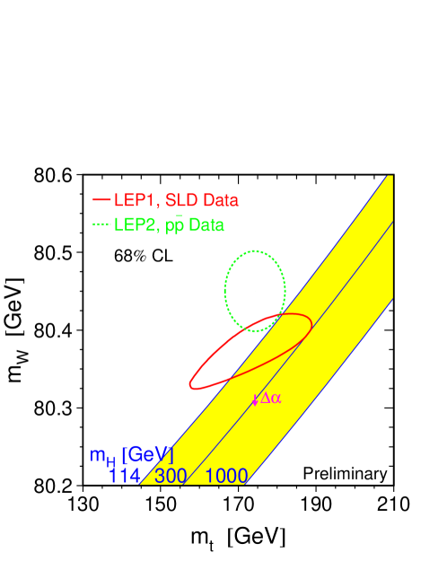
Figure 3: Lines of constant Higgs mass on a plot of $M_{W}$ vs. $m_{t}$. The dashed ellipse is the $68\%$ CL direct measurement of $M_{W}$ and $m_{t}$. The solid ellipse is the $68\%$ CL indirect measurement from precision electroweak data. From http://lepewwg.web.cern.ch/LEPEWWG.

I show in Fig. 3 a plot of $M_{W}$ vs. $m_{t}$, with lines of constant Higgs mass. The dashed ellipse is the $68\%$ CL region from direct measurements; the solid ellipse is the $68\%$ CL region from indirect measurements. The fact that these ellipses lie near each other, and near the lines of constant Higgs mass (for $m_{h}>114$ GeV) tells us that the standard model is not obviously wrong. It also indicates that the Higgs boson is light, $m_{h}<204$ GeV at $95\%$ CL Hagiwara:pw .

Before we become too smug about the success of the standard model in precision electroweak analyses, note that the fit to all data has a CL of 0.01, hardly confidence inspiring Chanowitz:2002cd . This is due to two anomalous measurements: the $b$ forward-backward asymmetry ($A_{FB}^{b}$) measured at LEP, which deviates by $2.6\sigma$, and $\sin^{2}\theta_{W}(\nu N)$ measured by the NuTeV collaboration Zeller:2001hh , which deviates by $3\sigma$. What if we (very unscientifically) discard these measurements from the global fit? Then we find that $m_{h}>114$ GeV has a CL of only 0.03, because these two measurements favor a heavy Higgs boson, while the other measurements favor a very light Higgs boson. If we only discard the NuTeV measurement, then the fit CL is 0.10, which is marginally acceptable. It seems that there is some tension in the fit of the precision electroweak data to the standard model.

Measurements of $M_{W}$ and $m_{t}$ at the Tevatron could resolve or exacerbate this tension. Let us take as a goal for Run IIa (2 fb^-1) uncertainties of $\Delta M_{W}=30$ MeV, $\Delta m_{t}=3$ GeV. Combined with the LEP measurement of $\Delta M_{W}=42$ MeV, the uncertainty in the $W$ mass would be $\Delta M_{W}=24$ MeV. The goals for Run IIb are $\Delta M_{W}=20$ MeV, $\Delta m_{t}=$ 2 GeV. These measurements will be important tests of the standard model, either increasing our confidence in it or indicating that there is physics beyond it.

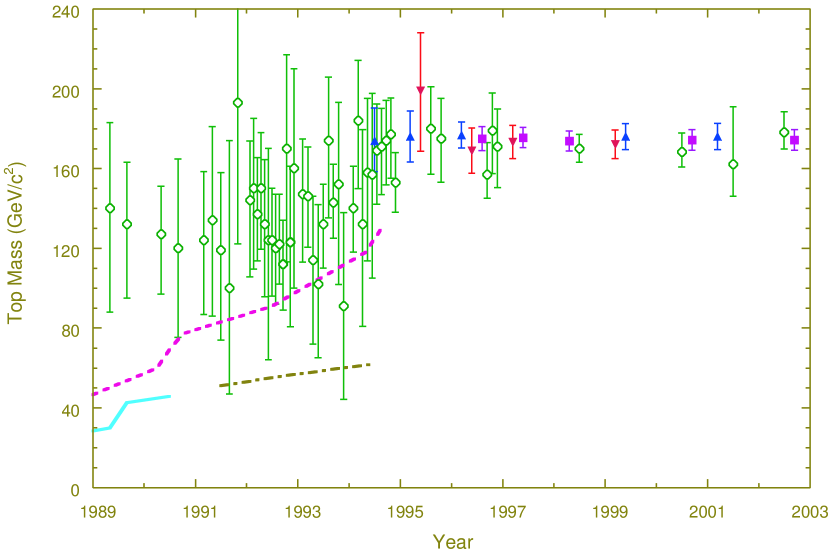
Figure 4: ($\diamondsuit$) Indirect bounds on the top-quark mass from precision electroweak data. ($\sqcap\!\!\!\!\sqcup$) World-average direct measurement of the top-quark mass; ($\bigtriangleup$) CDF and ($\bigtriangledown$) D0 measurements. Lower bounds from $p\bar{p}$ (dashed) and $e^{+}e^{-}$ (solid) colliders. Updated by C. Quigg from Ref. Quigg:fy .

Should we believe that the Higgs boson is light, as indicated by precision electroweak data? In defense of this, I show in Fig. 4 a plot of direct and indirect measurements of the top-quark mass versus time. Precision electroweak measurements anticipated $m_{t}<200$ GeV, which suggests that we should trust the prediction $m_{h}<200$ GeV.

2.2 CKM

The CKM elements involving the top quark have never been measured directly; they are inferred from the unitarity of the CKM matrix. Their values are Hagiwara:pw

$$|V_{td}|=0.004-0.014$$

$$|V_{ts}|=0.037-0.044$$

$$|V_{tb}|=0.9990-0.9993\;.$$

Thus $|V_{td}|$, $|V_{ts}|$, and $|V_{tb}|$ are known with a precision of $50\%$, $10\%$, and $0.02\%$, respectively. How can we measure these CKM elements?

Figure 5: $B_{d}^{0}-\bar{B}_{d}^{0}$ mixing proceeds via a box diagram.

$|V_{td}|$

This may be determined indirectly from $B_{d}^{0}-\bar{B}_{d}^{0}$ mixing, shown in Fig. 5. The frequency of oscillation, $\Delta m_{d}$, is proportional to $|V_{tb}^{*}V_{td}|^{2}$. Measurements give Hagiwara:pw

$$|V_{tb}^{*}V_{td}|=0.0079\pm 0.0015\;,$$ (10)

where the uncertainty ($20\%$) is almost entirely from the theoretical uncertainty in the hadronic matrix element. Assuming three generations ($|V_{tb}|\approx~{}1)$, this is a more accurate measurement of $|V_{td}|$ than can be inferred from unitarity ($50\%$).

$|V_{ts}|$

This may be determined indirectly from $B_{s}^{0}-\bar{B}_{s}^{0}$ mixing, which is the same as Fig. 5 but with the $d$ quark replaced by an $s$ quark. The frequency of oscillation, $\Delta m_{s}$, is proportional to $|V_{tb}^{*}V_{ts}|^{2}$. Thus far there is only a lower limit on the oscillation frequency,

$$\Delta m_{s}>14.4\,{\rm ps}^{-1}\;.$$ (11)

The anticipated value from the range of $|V_{ts}|$ listed above is $\Delta m_{s}\approx 18\,{\rm ps}^{-1}$, just above the current lower bound. This should be observable in Run II at the Tevatron. However, the theoretical uncertainty is very similar to that of $\Delta m_{d}$, which means that $|V_{ts}|$ can only be extracted with an uncertainty of $20\%$, which is greater than the uncertainty in the value inferred from unitarity ($10\%$).

$|V_{ts}|/|V_{td}|$

We can use the similarity in the hadronic matrix elements involved in $\Delta m_{s}$ and $\Delta m_{d}$ to our advantage by taking the ratio:

$$\frac{\Delta m_{s}}{\Delta m_{d}}=\frac{M_{B_{s}}}{M_{B_{d}}}\xi^{2}\left|\frac{V_{ts}}{V_{td}}\right|^{2}\;.$$ (12)

The theoretical uncertainty in the ratio of the hadronic matrix elements, $\xi^{2}$, is much less than the uncertainty in the hadronic matrix elements themselves. Using the value of $|V_{ts}|$ from unitarity yields an uncertainty in $|V_{td}|$ that is less than the uncertainty obtained from $\Delta m_{d}$ alone.

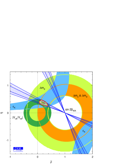
Figure 6: The $\bar{\rho}$-$\bar{\eta}$ plane, showing constraints from various measurements, as well as the best fit. From http://ckmfitter.in2p3.fr Hocker:2001xe .

I show in Fig. 6 the $\bar{\rho}$-$\bar{\eta}$ plane. The radius of the large circles centered at $(1,0)$ is proportional to $|V_{td}|$. The large annulus is from the measurement of $\Delta m_{d}$. The small annulus that lies inside it is from the ratio $\Delta m_{s}/\Delta m_{d}$ and $\Delta m_{d}$ combined, using the current lower bound on $\Delta m_{s}$. The measurement of $\Delta m_{s}$ at the Tevatron will reduce the width of this annulus by about a half, making it one of the most precise measurements in the $\bar{\rho}$-$\bar{\eta}$ plane.

$|V_{tb}|$

Despite the fact that it has never been measured directly, $|V_{tb}|$ is the best known CKM element ($0.02\%$), assuming three generations. It is only interesting to measure it if we relax the assumption of three generations, in which case $|V_{tb}|$ is almost completely unconstrained Hagiwara:pw ,

$$|V_{tb}|=0.08-0.9993\;.$$ (13)

How can we directly measure $|V_{tb}|$ in this scenario?

Figure 7: Top-quark decay to a $W$ boson and a light quark ($q=d,s,b$).

Let’s consider top-quark decay, shown in Fig. 7. CDF has measured the fraction of top decays that yield a $b$ quark Affolder:2000xb ,

$$\frac{BR(t\to Wb)}{BR(t\to Wq)} =0.94^{+0.31}_{-0.24}$$ (15)

$$=\frac{|V_{tb}|^{2}}{|V_{td}|^{2}+|V_{ts}|^{2}+|V_{tb}|^{2}}\;,$$

where $q$ denotes any light quark ($d,s,b$). The second line is the interpretation of this measurement in terms of CKM elements. If we were to assume three generations, the denominator of this expression would be unity, but we are not making that assumption. The fact that this fraction is close to unity only tells us that $|V_{tb}|\gg|V_{ts}|,|V_{td}|$; it does not tell us its absolute magnitude.

Figure 8: Single-top-quark production via the weak interaction: (a) $s$-channel process, (b) $t$-channel process.

The way to measure $|V_{tb}|$ directly, with no assumptions about the number of generations, is to measure top-quark production via the weak interaction Stelzer:1998ni . There are two relevant subprocesses at the Tevatron, shown in Fig. 8. The $s$-channel process proceeds via quark-antiquark annihilation and produces a $t\bar{b}$ final state. Turning this diagram on its side yields the $t$-channel process, in which the virtual $W$ boson strikes a $b$ quark in the proton sea and promotes it to a top quark. Both processes produce a single top quark in the final state, rather than a $t\bar{t}$ pair. The cross sections for these processes are proportional to $|V_{tb}|^{2}$, and thus provide a direct measurement of this CKM element. These processes should be observed in Run II, and yield a measurement of $|V_{tb}|$ with an uncertainty of about $10\%$.

2.3 Top quark

Figure 9: Top-quark pair production at the Tevatron proceeds principally via quark-antiquark annihilation, with a smaller contribution from $gg\to t\bar{t}$.

The strong and weak interactions of the top quark are not nearly as well studied as those of the other quarks and leptons. The strong interaction is most directly measured in top-quark pair production, shown in Fig. 9. The weak interaction is measured in top-quark decay, Fig. 7, and single-top-quark production, Fig. 8, discussed in the previous section.

The standard model predicts that the $W$ boson in top-quark decay will be dominantly longitudinally polarized,

$$BR(t\to W_{0}b)=\frac{m_{t}^{2}}{m_{t}^{2}+2M_{W}^{2}}\approx 0.70\;.$$ (16)

CDF has made the crude measurement $BR(t\to W_{0}b)=0.91\pm 0.37\pm 0.13$, consistent with the standard-model expectation Affolder:1999mp . This measurement should improve significantly in Run II.

Figure 10: (a) In $t\bar{t}$ production, the spins of the top quark and antiquark are $100\%$ correlated when measured along an axis that makes an angle $\psi$ with respect to the beam axis, where $\tan\psi=\beta^{2}\sin\theta\cos\theta/(1-\beta^{2}\sin^{2}\theta)$; (b) In single-top production, the top quark is $100\%$ polarized along the direction of motion of the $d$ quark, in the top-quark rest frame.

One of the unique features of the top quark is that it decays before there is time for its spin to be depolarized by the strong interaction. Thus the top-quark spin is directly observable via the angular distribution of its decay products. This means that we should be able to measure observables that depend on the top-quark spin.

In the production of $t\bar{t}$ pairs via the strong interaction, Fig. 9, the spins of the top quark and antiquark are $100\%$ correlated, as shown in Fig. 10(a) Mahlon:1997uc . In single-top production, the spin of the top quark is $100\%$ polarized along the direction of motion of the $d$ quark, in the top-quark rest frame, as shown in Fig. 10(b) Mahlon:1996pn . These spin effects should be observable in Run II.

2.4 Higgs boson

Figure 11: Higgs-boson production (a) in association with a weak vector boson, (b) via weak-vector-boson fusion.

As mentioned in the introduction to this section, the LHC was designed to discover the Higgs boson. However, there is a chance that the Tevatron could make this discovery first. The most promising channel is associated production of the Higgs boson with a $W$ or $Z$ boson, as shown in Fig. 11(a), followed by $h\to b\bar{b}$ Stange:ya . This channel is not considered viable at the LHC, so it is of particular interest to try to observe it at the Tevatron. Other discovery channels are associated production of the Higgs boson and a $t\bar{t}$ pair Goldstein:2000bp and, for higher Higgs-boson masses, Higgs-boson production via gluon fusion, followed by $h\to WW^{(*)}$ Han:1998ma .

Figure 12: Integrated luminosity required to discover ($5\sigma$), find evidence for ($3\sigma$), or rule out ($95\%$ CL) the Higgs boson at the Tevatron vs. the Higgs mass.

Figure 12 is the well-known plot of the integrated luminosity required to discover the Higgs boson ($5\sigma$), find evidence for it ($3\sigma$), or rule it out ($95\%$ CL) Carena:2000yx . If we take seriously the indication from precision electroweak physics that the Higgs boson is lighter than 200 GeV, then we will be unable to rule it out. To discover it, we will really need $5\sigma$ — this is the Higgs boson we are talking about! Given the lower bound $m_{h}>114$ GeV from LEP, this means we need 15 fb^-1 of integrated luminosity to get into the game.

The LHC can’t miss the Higgs boson. In addition to the production processes available at the Tevatron, there is also weak-vector-boson fusion, shown in Fig. 11(b), which was originally proposed for the discovery of a heavy Higgs boson. The potential of this process for the discovery of an intermediate-mass Higgs boson has recently been appreciated Rainwater:1998kj ; Rainwater:1999sd . Figure 13 shows the signal significance for the discovery of an intermediate-mass Higgs boson in a variety of channels. The importance of the weak-vector-boson-fusion channels is evident.

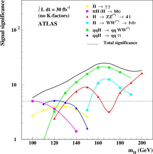
Figure 13: $S/\sqrt{B}$ for a variety of Higgs-boson production and decay channels at the LHC vs. the Higgs mass.

Once we discover the Higgs boson, we want to measure its couplings to other particles. The ratio of Higgs couplings can be extracted by measuring a variety of production and decay modes Zeppenfeld:2000td . Thus it is important to be able to see the Higgs boson in as many channels as possible. This again emphasizes the importance of the weak-vector-boson-fusion channels.

2.5 QCD

Perhaps it is surprising to see QCD in this list of ways in which the Tevatron can confront the standard model. After all, we know beyond the shadow of a doubt that QCD is the correct theory of the strong interaction. However, we don’t always know how to use it correctly. Here I discuss three aspects of the confrontation between theory and experiment in QCD.

$J/\psi$ production

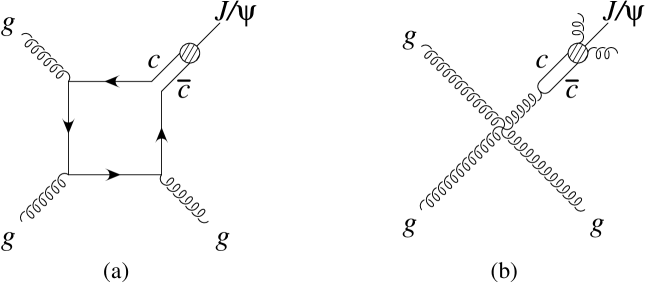
Figure 14: $J/\psi$ production at high transverse momentum: (a) color-singlet mechanism, (b) color-octet mechanism.

Figure 15: $J/\psi$ transverse momentum distribution at the Tevatron. The LO color-singlet contribution corresponds to Fig. 14(a); the color-octet ${}^{3}S_{1}$ contribution corresponds to Fig. 14(b). From Ref. Kramer:2001hh .

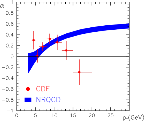
Figure 16: Polarization of $J/\psi$ as a function of its transverse momentum. The data are compared with the prediction from the process in Fig. 14(b) and related processes.

It was long thought that $J/\psi$ production at high transverse momentum proceeds via the process shown in Fig. 14(a), in which a color-singlet $c\bar{c}$ pair is produced. However, this process yields a cross section that is more than an order of magnitude too small, and has the wrong transverse-momentum dependence, as shown by the curve labeled “LO color-singlet” in Fig. 15. We now believe that the dominant production mechanism at high transverse momentum involves a gluon that produces a color-octet $c\bar{c}$ pair, which then fragments into a $J/\psi$ by emitting two or more soft gluons, as shown in Fig. 14(b) Braaten:1994vv . For a suitable choice of the hadronic matrix element that parameterizes the fragmentation function, this gives a good description of the data, as shown in Fig. 15. This mechanism also makes an unambiguous prediction: the $J/\psi$ should be transversely polarized at high transverse momentum, since it is emanating from a gluon, which has only transverse polarization states. The predicted polarization is shown in Fig. 16, along with data from Run I; the agreement is hardly encouraging Affolder:2000nn . The data from Run II will put this to a decisive test, and tell us if we need to go back to the drawing board in order to explain $J/\psi$ production at high transverse momentum.

$b$ production

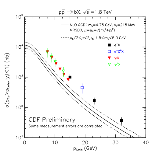
Figure 17: The $b$-quark cross section vs. the minimum transverse momentum of the $b$ quark. From http://www-cdf.fnal.gov/physics/new/bottom/bottom.html.

Another area in which the agreement between theory and experiment is less than impressive is $b$-quark production. The data lie significantly above the prediction of next-to-leading-order QCD Nason:1989zy ; Beenakker:1988bq , as shown in Fig. 17. A similar excess has been observed at HERA ($\gamma^{*}g\to b\bar{b}$) and at LEP ($\gamma^{*}\gamma^{*}\to b\bar{b}$). This has stimulated a great deal of work on QCD, but there is not yet a generally-accepted resolution of this conundrum. The slightly-higher energy of Run II provides another venue in which to test our theoretical ideas against experiment.

Multijet production

Multijet production is interesting in its own right, and also as a background to new physics. In order to recognize physics beyond the standard model, we must first be able to calculate standard-model processes with reasonable precision. Multijet production (by itself or together with other particles) is difficult to calculate even at tree level, and challenges our ability to calculate efficiently.

There are two new general-purpose tools available for such calculations: ALPGEN Mangano:2002ea and MadEvent Maltoni:2002qb . They are both leading-order event generators, with color information that allows them to be merged with shower Monte Carlo codes. Each has its own strengths, so I invite you to take them out for a test drive. Currently neither code can produce generic multijet events with more than six jets, but that should change in the near future. One promising new development in the calculation of multiparton amplitudes is the color-flow decomposition; the subprocess cross section for $gg\to 10g$ has recently been evaluated using this method Maltoni:2002mq .

3 Beyond the Standard Model

As discussed in Section 1, the standard model is a simple, elegant, and successful theory. Why should we even contemplate physics beyond the standard model? It almost seems ungrateful. The situation is in some ways analogous to that of classical physics in the 1890’s, which seemed to explain almost all known phenomena. However, that decade witnessed the discovery of X-rays by Röntgen, radioactivity by Becquerel, and the electron by Thomson, and it soon became clear that these could not be understood in terms of classical physics. These discoveries and others eventually led to the theories of quantum mechanics and relativity, upon which the standard model is based. The question I would like to address is: What are the analogous anomalies today? Below I list both direct and indirect evidence for physics beyond the standard model.

3.1 Direct evidence

Neutrinos

Recall that in our review of the standard model we restricted ourselves to the simplest possible interactions, but we did not explain why we imposed this restriction. The most conservative (and most plausible) explanation is that additional interactions are present, but they are suppressed. If we were to add these additional interactions, we would find (via dimensional analysis) that they have coefficients with dimensions of an inverse power of mass Willenbrock:2002ta ,

$${\cal L}={\cal L}_{SM}+\frac{1}{M}{\cal L}_{5}+\frac{1}{M^{2}}{\cal L}_{6}+\cdots$$ (17)

where $M$ is a mass scale greater than the Higgs-field vacuum-expectation value, $v$. At energies much less than $M$, the least-suppressed interactions come from the Lagrangian labeled ${\cal L}_{5}$. Remarkably, there is one and only one possible term in this Lagrangian (assuming the standard-model particle content) Willenbrock:2002ta ; Weinberg:sa ,

$${\cal L}_{5}=c^{ij}(L_{L}^{iT}\epsilon\phi)C(\phi^{T}\epsilon L_{L}^{j})+h.c.\;.$$ (18)

where $L_{L}$ and $\phi$ are the lepton and Higgs-doublet fields (see Table 1) [$C$ is the charge-conjugation matrix]. When the Higgs field acquires a vacuum-expectation value, this term gives rise to a Majorana mass matrix for the neutrinos,

$$M_{\nu}^{ij}=c^{ij}\frac{v^{2}}{M}.$$ (19)

Thus we expect neutrino masses and mixing, with masses much less than $v$ (for $M\gg v$). The observation of neutrino oscillations is thus unambiguous evidence of physics beyond the standard model.

Gravity

Although we don’t always think of it this way, gravity is definitely beyond the standard model. If we add a graviton field, $g_{\mu\nu}$, to the theory, the least-suppressed additional interactions (using dimensional analysis) are

$${\cal L}_{gravity}=\frac{M_{P}^{2}}{16\pi}\sqrt{-g}(-2\Lambda+R+\cdots)$$ (20)

where $M_{P}$ is the Planck scale, $g\equiv{\rm det}\;g^{\mu\nu}$, $R$ is the Ricci scalar, and $\Lambda$ is the cosmological constant. The Ricci-scalar term accounts for all of classical gravity. The cosmological constant, long thought to be exactly zero, is able to account for the mysterious “dark energy” needed to accommodate cosmological observations.

Astrophysics and Cosmology

Along with the dark energy mentioned above, which is believed to account for about $60\%$ of the mass-energy of the universe, there is also “dark matter”, whose nature is unknown, which accounts for about $35\%$ of the mass-energy. Whatever this matter is, it is certainly beyond the standard model. The observed baryon asymmetry of the universe also cannot be explained by the standard model, because it requires a source of CP violation beyond that contained in the CKM matrix. The inflationary model of the universe, so successful in explaining many of the features of our universe, also requires physics beyond the standard model.

Precision electroweak

As discussed in Section 2.1, precision electroweak data may already be indicating physics beyond the standard model. Future measurements may strengthen or weaken this evidence.

3.2 Indirect evidence

Masses and mixing angles

The standard model accommodates generic masses and mixing angles, but the observed values are far from generic. The natural scale of charged fermion masses is of order $v$, but all charged fermions (except the top quark) are much lighter than this, and display a hierarchical pattern. The CKM mixing angles are also not generic; they are small, and are also hierarchical. These facts suggest that there is physics beyond the standard model that explains the pattern of charged fermion masses and mixing. Unfortunately, the standard model does not indicate at what energy scale this new physics resides Maltoni:2001dc .

Grand Unification

SU(5) grand unification is a lovely idea Georgi:sy , but it is ruled out; now that we know the gauge couplings with good accuracy, we find that they do not unify at high energies. It is remarkable that by imposing weak-scale supersymmetry on the theory, the relative evolution of the couplings is nudged just enough to successfully unify the couplings at the scale $M_{GUT}\approx 10^{16}$ GeV. This suggests that the supersymmetric partners of the known particles await us as we probe the weak scale.

Hierarchy problems

Recall that the standard model has only one energy scale, the Higgs-field vacuum-expectation value, $v$. Why is $v\ll M_{P},M_{GUT}$? Why is $\Lambda\ll M_{P}^{2},v^{2}$? In other words, why does it appear that physics beyond the standard model is associated with scales wildly different from $v$? Perhaps the explanation for this requires yet more physics beyond the standard model, such as supersymmetry or large extra dimensions.

It is striking that almost all of these anomalies and hints of physics beyond the standard model involve the Higgs field in one way or another. Neutrino masses involve the Higgs field, via Eq. (18); the vacuum-expectation value of the Higgs field contributes to the cosmological constant; the axion (a type of Higgs field) is a dark-matter candidate; there could be additional CP violation in the Higgs sector that generates the baryon asymmetry; the inflaton (a scalar field) could drive inflation; precision electroweak data constrain the Higgs sector; fermion masses and mixing angles result from the coupling of the Higgs field to fermions, Eq. (4); SUSY SU(5) grand unification requires two Higgs doublets; and the hierarchy problems involve the Higgs-field vacuum-expectation value.

The conclusion I would like to draw from these observations is that discovering and studying the Higgs boson (or bosons) is central to understanding physics beyond the standard model. We should be on the lookout for two (or more) Higgs doublets; Higgs singlets or triplets; Higgs-sector CP violation; alternative models of electroweak symmetry breaking; composite Higgs bosons, etc. If we are lucky, we will begin to probe this physics at the Tevatron; we are guaranteed to learn something about it at the LHC. We look forward to an exciting era of physics associated with electroweak symmetry breaking and physics beyond the standard model.

References

- (1) S. Willenbrock, to appear in the Proceedings of the Advanced Study Institute on Techniques and Concepts of High Energy Physics, St. Croix, U. S. Virgin Islands, June 13–24, 2002, arXiv:hep-ph/0211067.
- (2) K. Hagiwara et al. [Particle Data Group Collaboration], Phys. Rev. D 66, 010001 (2002).
- (3) M. S. Chanowitz, Phys. Rev. D 66, 073002 (2002) [arXiv:hep-ph/0207123].
- (4) G. P. Zeller et al. [NuTeV Collaboration], Phys. Rev. Lett. 88, 091802 (2002) [arXiv:hep-ex/0110059].
- (5) C. Quigg, Phys. Today 50N5, 20 (1997).
- (6) A. Hocker, H. Lacker, S. Laplace and F. Le Diberder, Eur. Phys. J. C 21, 225 (2001) [arXiv:hep-ph/0104062].
- (7) T. Affolder et al. [CDF Collaboration], Phys. Rev. Lett. 86, 3233 (2001) [arXiv:hep-ex/0012029].
- (8) T. Stelzer, Z. Sullivan and S. Willenbrock, Phys. Rev. D 58, 094021 (1998) [arXiv:hep-ph/9807340].
- (9) T. Affolder et al. [CDF Collaboration], Phys. Rev. Lett. 84, 216 (2000) [arXiv:hep-ex/9909042].
- (10) G. Mahlon and S. Parke, Phys. Lett. B 411, 173 (1997) [arXiv:hep-ph/9706304].
- (11) G. Mahlon and S. Parke, Phys. Rev. D 55, 7249 (1997) [arXiv:hep-ph/9611367].
- (12) A. Stange, W. J. Marciano and S. Willenbrock, Phys. Rev. D 49, 1354 (1994) [arXiv:hep-ph/9309294].
- (13) J. Goldstein, C. S. Hill, J. Incandela, S. Parke, D. Rainwater and D. Stuart, Phys. Rev. Lett. 86, 1694 (2001) [arXiv:hep-ph/0006311].
- (14) T. Han and R. J. Zhang, Phys. Rev. Lett. 82, 25 (1999) [arXiv:hep-ph/9807424].
- (15) M. Carena et al., “Report of the Tevatron Higgs Working Group,” arXiv:hep-ph/0010338.
- (16) D. Rainwater, D. Zeppenfeld and K. Hagiwara, Phys. Rev. D 59, 014037 (1999) [arXiv:hep-ph/9808468].
- (17) D. Rainwater and D. Zeppenfeld, Phys. Rev. D 60, 113004 (1999) [Erratum-ibid. D 61, 099901 (2000)] [arXiv:hep-ph/9906218].
- (18) D. Zeppenfeld, R. Kinnunen, A. Nikitenko and E. Richter-Was, Phys. Rev. D 62, 013009 (2000) [arXiv:hep-ph/0002036].
- (19) E. Braaten and S. Fleming, Phys. Rev. Lett. 74, 3327 (1995) [arXiv:hep-ph/9411365].
- (20) M. Kramer, Prog. Part. Nucl. Phys. 47, 141 (2001) [arXiv:hep-ph/0106120].
- (21) T. Affolder et al. [CDF Collaboration], Phys. Rev. Lett. 85, 2886 (2000) [arXiv:hep-ex/0004027].
- (22) P. Nason, S. Dawson and R. K. Ellis, Nucl. Phys. B 327, 49 (1989) [Erratum-ibid. B 335, 260 (1990)].
- (23) W. Beenakker, H. Kuijf, W. L. van Neerven and J. Smith, Phys. Rev. D 40, 54 (1989).
- (24) M. L. Mangano, M. Moretti, F. Piccinini, R. Pittau and A. D. Polosa, arXiv:hep-ph/0206293.
- (25) F. Maltoni and T. Stelzer, arXiv:hep-ph/0208156.
- (26) F. Maltoni, K. Paul, T. Stelzer and S. Willenbrock, arXiv:hep-ph/0209271.
- (27) S. Weinberg, Phys. Rev. Lett. 43, 1566 (1979).
- (28) F. Maltoni, J. M. Niczyporuk and S. Willenbrock, Phys. Rev. D 65, 033004 (2002) [arXiv:hep-ph/0106281].
- (29) H. Georgi and S. L. Glashow, Phys. Rev. Lett. 32, 438 (1974).