Abstract

The aim of this review is to demonstrate that there exists a coherent picture of strong interactions, based on instantons. Starting from the first principles of Quantum Chromodynamics – via the microscopic mechanism of spontaneous chiral symmetry breaking – one arrives to a quantitative description of the properties of light hadrons, with no fitting parameters. The discussion of the importance of instanton-induced interactions in soft high-energy scattering is new.

1 Introduction

Strong interactions as described by Quantum Chromodynamics (QCD) is a remarkable branch of physics where the observable entities – hadrons and nuclei – are very far from quarks and gluons in terms of which the theory is formulated. To make matters worse, the scale of strong interactions 1 fm is nowhere to be found in the QCD Lagrangian. If we restrict ourselves to hadrons ‘made of’ $u,d,s$ quarks and glue, the masses of those quarks can be to a good accuracy set to zero. In this so-called chiral limit the nucleon is just 5% lighter than in reality. In the chiral limit there is not a single dimensional parameter in the QCD Lagrangian. The 1 fm scale surfaces via a mechanism named the ‘transmutation of dimensions’. QCD is a quantum field theory and beeing such it is not defined without introducing of some kind of ultra-violet cutoff $\mu$. There is also a dimensionless gauge coupling constant given at that cutoff $\alpha_{s}(\mu)$. The dimensionful quantity $\Lambda$ determining the scale of the strong interactions is the combination of $\mu$ and $\alpha_{s}(\mu)$:

$$\Lambda = \mu\,\exp\left(-\frac{2\pi}{b_{1}\alpha_{s}(\mu)}\right)\,\left(\frac{4\pi}{b_{1}\alpha_{s}(\mu)}\right)^{\frac{b_{2}}{2b_{1}^{2}}}\,\left(1+O\left(\alpha_{s}\right)\right),$$ (1.1)

$$b_{1} = \frac{11}{3}N_{c}-\frac{2}{3}N_{f},\qquad b_{2}=\frac{34}{3}N_{c}^{2}-\frac{13}{3}N_{c}N_{f}+\frac{N_{f}}{N_{c}},$$ (1.2)

where $N_{c}=3$ is the number of quark colours and $N_{f}$ is the number of acting quark flavours. The ultra-violet cutoff $\mu$ sets in the dimension of mass but the exponentially small factor makes $\Lambda$ much less than $\mu$. To ensure that $\Lambda$ is actually independent of the cutoff, one has to add that $\alpha_{s}(\mu)$ has to decrease with $\mu$ according to

$$\frac{2\pi}{\alpha_{s}(\mu)}=b_{1}\ln\frac{\mu}{\Lambda}+\frac{b_{2}}{2b_{1}}\ln\ln\frac{\mu^{2}}{\Lambda^{2}}+O\left(\frac{1}{\ln\frac{\mu}{\Lambda}}\right).$$ (1.3)

This formula is called ‘asymptotic freedom’: at large scales $\alpha_{s}$ decreases.

All physical observables in strong interactions, like the nucleon mass, the pion decay constant $F_{\pi}$, total cross sections, etc. are proportioal to $\Lambda$ in the appropriate power. That is how the strong interactions scale, 1 fm, appears in the theory. One of the theory’s goals is to get, say, the nucleon mass in the form of eq. (1.1) and to find the numerical proportionality coefficient. Doing lattice simulations the first thing one needs to check is whether an observable scales with $\alpha_{s}$ as prescribed by eq. (1.1). If it does not, the continuum limit is not achieved. In analytical approaches, getting an observable in the form of eq. (1.1) is extremely difficult. It implies doing non-perturbative physics. The only analytical approach to QCD I know of where one indeed gets observables through the transmutation of dimensions is the approach based on instantons, and it will be the subject of this paper.

Instantons are certain large non-perturbative fluctuations of the gluon field discovered by Belavin, Polyakov, Schwartz and Tyupkin in 1975 [1, 2], and the name has been suggested in 1976 by ’t Hooft [3], who made a major contribution to the investigation of the instantons properties. The QCD instanton vacuum has been studied starting from the pioneering works in the end of the seventies [4, 5]; a quantitative treatment of the instanton ensemble has been developed in refs. [6, 7]. The basic ideas of the instanton vacuum are presented in section 2.

Instantons are not the only possible large non-perturbative fluctuations of the gluon field: one can think also of merons, monopoles, vortices, etc. I briefly review that in section 3 where also certain new material on dyons is presented. However, instantons are the best studied non-perturbative effects. It may happen that they are not the whole truth but they are definitely present in the QCD vacuum, and they are working quite effectively in reproducing many remarkable features of the strong interactions. For example, instantons lead to the formation of the gluon condensate [8] and of the so-called topological susceptibility needed to cure the $U(1)$ paradox [3, 9]. The most striking success of instantons is their capacity to provide a beautiful microscopic mechanism of the spontaneous chiral symmetry breaking [10, 11, 12, 13]. Moreover, instantons enable one to understand it from different angles and using different mathematical formalisms. These topics are central in the review and are presented in sections 4,5 and 6.

We know that, were the chiral symmetry of QCD unbroken, the lightest hadrons would appear in parity doublets. The large actual splitting between, say, $N(\frac{1}{2}^{-},1535)$ and $N(\frac{1}{2}^{+},940)$ implies that chiral symmetry is spontaneously broken as characterized by the nonzero quark condensate $<\!\bar{\psi}\psi\!>\simeq-(250\,{\rm MeV})^{3}$. Equivalently, it means that nearly massless (‘current’) quarks obtain a sizable non-slash term in the propagator, called the dynamical or constituent mass $M(p)$, with $M(0)\simeq 350\,{\rm MeV}$. The $\rho$-meson has roughly twice and nucleon thrice this mass, i.e. are relatively loosely bound. The pion is a (pseudo) Goldstone boson and is very light. The hadron size is typically $\sim 1/M(0)$ whereas the size of constituent quarks is given by the slope of $M(p)$. In the instanton approach the former is much larger than the latter. It explains, at least on the qualitative level, why constituent quark models are so phenomenologically successful.

It should be stressed that literally speaking instantons do not lead to confinement, although they induce a growing potential for heavy quarks at intermediate separations [14]; asymptotically it flattens out [4]. However, it has been realized long ago [5, 15], that it is chiral symmetry breaking and not confinement that determines the basic characteristics of nucleons and pions as well as their first excitations. After all, 99% of the mass around us is due to the spontaneous generation of the quark constituent mass. Probably one would need an explicit confinement to get the properties of short-living highly excited hadrons. According to a popular wisdom, moving a quark away from a diquark system in a baryon generates a string, also called a flux tube, whose energy rises linearly with the separation. This is expected in the “pure-glue” world with no dynamical quarks. However, in the real world with light quarks and the spontaneous chiral symmetry breaking the string energy exceeds the pion mass $m_{\pi}=140\,{\rm MeV}$ at a modest separation of about $0.26\,{\rm fm}$, see Fig. 1. At larger separations the would-be linear potential is screened since it is energetically favourable to tear the string and produce a pion. Virtually, the linear potential can stretch to as much as $0.4\,{\rm fm}$ where its energy exceeds $2m_{\pi}$ but that can happen only for a short time of $1/m_{\pi}$. Meanwhile, the ground-state baryons are stable, and their sizes are about $1\,{\rm fm}$. The pion-nucleon coupling is huge, and there seems to be no suppression of the string breaking by pions. The paradox is that the linear potential of the pure glue world, important as it might be to explain why quarks are not observed as a matter of principle, can hardly have a direct impact on the properties of lightest hadrons.

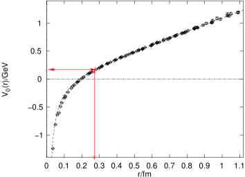
Figure 1: The lattice-simulated potential between static quarks in pure glue theory [16] exceeds $m_{\pi}$ at the separation of $0.26\,{\rm fm}$ (left). The screening of the linear potential by dynamical quarks is clearly seen in simulations at high temperatures but below the phase transition [17] (right). As one lowers the pion mass the string breaking happens at smaller distances; the scale is $\sqrt{\sigma}\simeq 425\,{\rm MeV}\simeq(0.47\,{\rm fm})^{-1}$.

Even for highly excited hadrons lying on linear Regge trajectories the situation is not altogether clear. The usual explanation of resonances lying on linear trajectories is that they are rotating confining flux tubes attached to quarks at end points moving with the speed of light. Why should $350\,{\rm MeV}$ quarks bound by a $\sqrt{\sigma}\simeq 425\,{\rm MeV}$ string move with the speed of light is not clear, but if they do not, the trajectories are not linear. In this picture, the finite (and experimentally large) width of resonances is due to the same string breaking by meson production. However, if there is no string in the ground-state nucleon, why should it be excited in a collision? The lightest degrees of freedom in the real world are pions and one might expect that they are the first to be excited. An alternative explanation of resonances lying on linear trajectories is that they are rotating elongated lumps of pion field [18], and their decay is due to the normal pion radiation. It follows then that the dominant decay of a large-J baryon resonance is a cascade ${\rm Bar}_{J}\to{\rm Bar}_{J-1}+\pi\to{\rm Bar}_{J-2}+\pi\pi\to...$ whereas if it is due to the string breaking it rather has a different pattern ${\rm Bar}_{J}\to{\rm Bar}_{\sim J/2}+{\rm Mes}_{\sim J/2}$. Studying the decay patterns of high-J resonances could be illuminating for understanding the relation between confining and chiral forces.

Leaving aside the unsettled question of highly excited resonances, the situation with the lightest and most important hadrons $\pi,\rho,N,\Delta$… is, to my mind, clear: it is the spontaneous chiral symmetry breaking (SCSB) rather than the expected linear confining potential of the pure glue world which is the key to understanding of their properties. Therefore, since the instanton vacuum describes successfully the physics of the chiral symmetry breaking, one would expect that instantons do explain the properties of light hadrons, both mesons and baryons. Indeed, a detailed numerical study of dozens of correlation functions with different quantum numbers in the instanton medium undertaken by Shuryak, Verbaarschot and Schäfer [19] (earlier certain correlation functions were computed analytically in refs. [11, 12]) demonstrated an impressing agreement with the phenomenology [20] and with direct lattice measurements [21], see ref. [22] for a review. In fact, instantons induce strong interactions between quarks, leading to bound-state baryons with calculable and reasonable properties. There are specialized reviews on this subject, therefore I touch it only briefly here (sections 8 and 9).

More recently, there has been much activity in applying instantons to explain various phenomena in high energy processes including heavy ion collisions. For that reason, I have included section 7 which suggests a new point of view on the pomeron which might be also related to instantons.

2 What are instantons?

2.1 Periodicity of the Yang–Mills potential energy

Being a quantum field theory, QCD deals with the fluctuating gluon and quark fields. A fundamental fact [23, 24] is that the potential energy of the gluon field is a periodic function in one particular direction in the infinite-dimensional functional space; in all other directions the potential energy is oscillator-like. This is illustrated in Fig. 2.

To observe this periodicity, let us temporarily work in the $A_{0}^{a}=0$ gauge, called Weyl or Hamiltonian gauge, and forget about fermions for a while. The remaining pure Yang–Mills or “pure glue” theory is nonetheless non-trivial, since gluons are self-interacting. For simplicity I start from the $SU(2)$ gauge group.

The spatial YM potentials $A_{i}^{a}({\bf x},t)$ can be considered as an infinite set of the coordinates of the system, where $i=1,2,3,\;\;a=1,2,3$ and ${\bf x}$ are “labels” denoting various coordinates. The YM action is

$$S=\frac{1}{4g^{2}}\int\!d^{4}x\;F_{\mu\nu}^{a}F_{\mu\nu}^{a}=\int dt\left(\frac{1}{2g^{2}}\int\!d^{3}{\bf x}\;{\bf E}^{2}-\frac{1}{2g^{2}}\int\!d^{3}{\bf x}\;{\bf B}^{2}\right)$$ (2.1)

where ${\bf E}$ is the electric field stregth,

$$E_{i}^{a}({\bf x},t)={\dot{A}}_{i}^{a}({\bf x},t)$$ (2.2)

(the dot stands for the time derivative), and ${\bf B}$ is the magnetic field stregth,

$$B_{i}^{a}({\bf x},t)=\frac{1}{2}\epsilon_{ijk}\left(\partial_{j}A_{k}^{a}-\partial_{k}A_{j}^{a}+\epsilon^{abc}A_{j}^{b}A_{k}^{c}\right).$$ (2.3)

Apparently, the first term in eq. (2.1) is the kinetic energy of the system of coordinates $\{A_{i}^{a}({\bf x},t)\}$ while the second term is minus the potential energy being just the magnetic energy of the field. The simple and transparent form of eq. (2.2) is the advantage of the Weyl gauge. Upon quantization the electric field is replaced by the variational derivative, $E_{i}^{a}(x)\rightarrow-ig^{2}\delta/\delta A_{i}^{a}(x)$, if one uses the ‘coordinate representation’ for the wave functional. The functional Schrödinger equation for the wave functional $\Psi[A_{i}^{a}(x)]$ takes the form

$${\cal H}\Psi[A_{i}]=\int\!d^{3}x\left\{-\frac{g^{2}}{2}\frac{\delta^{2}}{(\delta A_{i}^{a}(x))^{2}}+\frac{1}{2g^{2}}(B_{i}^{a}(x))^{2}\right\}\Psi[A_{i}]={\cal E}\Psi[A_{i}]$$ (2.4)

where ${\cal E}$ is the eigenenergy of the state in question. The YM vacuum is the ground state of the Hamiltonian (2.4), corresponding to the lowest energy ${\cal E}$.

Let us introduce an important quantity called the Pontryagin index or the four-dimensional topological charge of the YM fields:

$$Q_{T}=\frac{1}{32\pi^{2}}\int d^{4}x\;F_{\mu\nu}^{a}{\tilde{F}}_{\mu\nu}^{a},\qquad{\tilde{F}}_{\mu\nu}^{a}\equiv\frac{1}{2}\epsilon_{\mu\nu\alpha\beta}F_{\alpha\beta}^{a}.$$ (2.5)

The integrand in eq. (2.5) happens to be a full derivative of the four-vector $K_{\mu}$:

$$\frac{1}{32\pi^{2}}F_{\mu\nu}^{a}{\tilde{F}}_{\mu\nu}^{a}=\partial_{\mu}K_{\mu},\qquad K_{\mu}=\frac{1}{16\pi^{2}}\epsilon_{\mu\alpha\beta\gamma}\left(A_{\alpha}^{a}\partial_{\beta}A_{\gamma}^{a}+\frac{1}{3}\epsilon^{abc}A_{\alpha}^{a}A_{\beta}^{b}A_{\gamma}^{c}\right).$$ (2.6)

Therefore, assuming the fields $A_{\mu}$ are decreasing rapidly enough at spatial infinity, one can rewrite the 4-dimensional topological charge (2.5) as

$$Q_{T}=\int d^{4}x(\partial_{0}K_{0}-\partial_{i}K_{i})=\int dt\frac{d}{dt}\int d^{3}{\bf x}K_{0}.$$ (2.7)

Introducing the Chern–Simons number

$$N_{CS}=\int d^{3}{\bf x}\;K_{0}=\frac{1}{16\pi^{2}}\int d^{3}{\bf x}\>\epsilon^{ijk}\left(A_{i}^{a}\partial_{j}A_{k}^{a}+\frac{1}{3}\epsilon^{abc}A_{i}^{a}A_{j}^{b}A_{k}^{c}\right)$$ (2.8)

we see from eq. (2.7) that $Q_{T}$ can be rewritten as the difference of the Chern–Simons numbers characterizing the fields at $t=\pm\infty$:

$$Q_{T}=N_{CS}(+\infty)-N_{CS}(-\infty).$$ (2.9)

The Chern–Simons number of the field has an important property that it can change by integers under large gauge transformations. Indeed, under a general time-independent gauge transformation,

$$A_{i}\rightarrow U^{\dagger}A_{i}U+iU^{\dagger}\partial_{i}U,\;\;\;A_{i}\equiv A_{i}^{a}\frac{\tau^{a}}{2},$$ (2.10)

the Chern–Simons number transforms as follows:

$$N_{CS}\rightarrow N_{CS}+N_{W}+\frac{i}{8\pi^{2}}\int\!d^{3}x\,\epsilon^{ijk}\partial_{j}\,{\rm Tr}\,(\partial_{i}UU^{\dagger}A_{k}).$$ (2.11)

The last term is a full derivative and can be omitted if, e.g., $A_{i}$ decreases sufficiently fast at spatial infinity. $N_{W}$ is the winding number of the gauge transformation (2.10):

$$N_{W}=\frac{1}{24\pi^{2}}\int d^{3}{\bf x}\;\epsilon^{ijk}\left[(U^{\dagger}\partial_{i}U)(U^{\dagger}\partial_{j}U)(U^{\dagger}\partial_{k}U)\right].$$ (2.12)

The $SU(2)$ unitary matrix $U$ of the gauge transformation (2.10) can be viewed as a mapping from the 3-dimensional space onto the 3-dimensional sphere of parameters $S^{3}$. If at spatial infinity we wish to have the same matrix $U$ independently of the way we approach the infinity (and this is what is usually assumed), then the spatial infinity is in fact one point, so the mapping is topologically equivalent to that from $S^{3}$ to $S^{3}$. This mapping is known to be non-trivial, meaning that mappings with different winding numbers are irreducible by smooth transformations to one another. The winding number of the gauge transformation is, analytically, given by eq. (2.12). As it is common for topological characteristics, the integrand in (2.12) is in fact a full derivative. For example, if we take the matrix $U({\bf x})$ in a “hedgehog” form, $U=\exp[i(r\cdot\tau)/r\,P(r)]$, eq. (2.12) can be rewritten as

$$N_{W}=\frac{2}{\pi}\int\!dr\frac{dP}{dr}\sin^{2}P=\frac{1}{\pi}\left[P-\frac{\sin 2P}{2}\right]_{0}^{\infty}=\mbox{integer}$$ (2.13)

since $P(r)$ both at zero and at infinity needs to be multiples of $\pi$ if we wish $U(\vec{r})$ to be unambigiously defined at the origin and at the infinity.

Let us return now to the potential energy of the YM fields,

$${\cal V}=\frac{1}{2g^{2}}\int d^{3}{\bf x}\left(B_{i}^{a}\right)^{2}.$$ (2.14)

One can imagine plotting the potential energy surfaces over the Hilbert space of the coordinates $A_{i}^{a}({\bf x})$. It will be some complicated mountain country. If the field happens to be a pure gauge, $A_{i}=iU^{\dagger}\partial_{i}U$, the potential energy at such points of the Hilbert space is naturally zero. Imagine that we move along the “generalized coordinate” being the Chern–Simons number (2.8), fixing all other coordinates whatever they are. Let us take some point $A_{i}^{a}({\bf x})$ with the potential energy ${\cal V}$. If we move to another point which is a gauge transformation of $A_{i}^{a}({\bf x})$ with a winding number $N_{W}$, its potential energy will be exactly the same as it is strictly gauge invariant. However the Chern–Simons “coordinate” of the new point will be shifted by an integer $N_{W}$ from the original one. We arrive to the conclusion first pointed out by Faddeev [23] and Jackiw and Rebbi [24] in 1976, that the potential energy of the YM fields is periodic in the particular coordinate called the Chern–Simons number.

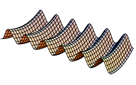
Figure 2: Potential energy of the gluon field is periodic in one direction and oscillator-like in all other directions in functional space.

2.2 Instantons in simple words

In perturbation theory one deals with zero-point quantum-mechanical fluctuations of the YM fields near one of the minima, say, at $N_{CS}=0\;$. The non-linearity of the YM theory is taken into account as a perturbation, and results in series in $g^{2}$ where $g$ is the gauge coupling. In that approach one is apparently missing a possibility for the system to tunnel to another minimum, say, at $N_{CS}=1\;$. The tunneling is a typical non-perturbative effect in the coupling constant.

Instanton is a large fluctuation of the gluon field in imaginary (or Euclidean) time corresponding to quantum tunneling from one minimum of the potential energy to the neighbour one. Mathematically, it was discovered by Belavin, Polyakov, Schwarz and Tyupkin; [1] the tunneling interpretation was given by V. Gribov, see [2]. The name ‘instanton’ has been introduced by ’t Hooft [3] who studied many of the key properties of those fluctuations. Anti-instantons are similar fluctuations but tunneling in the opposite direction in Fig. 2. Physically, one can think of instantons in two ways: on the one hand it is a tunneling process occuring in time, on the other hand it is a localized pseudoparticle in the Euclidean space.

Following the WKB approximation, the tunneling amplitude can be estimated as $\exp(-S)$, where $S$ is the action along the classical trajectory in imaginary time, leading from the minimum at $N_{CS}=0\;$at $t=-\infty$ to that at $N_{CS}=1\;$at $t=+\infty$. According to eq. (2.9) the 4-dimensional topological charge of such trajectory is $Q_{T}=1$. To find the best tunneling trajectory having the largest amplitude one has thus to minimize the YM action (2.1) provided the topological charge (2.5) is fixed to be unity. This can be done using the following trick [1]. Consider the inequality

$$0\leq\int d^{4}x\left(F_{\mu\nu}^{a}-{\tilde{F}}_{\mu\nu}^{a}\right)^{2}$$

$$=\int d^{4}x\left(2F^{2}-2F{\tilde{F}}\right)=8g^{2}S-64\pi^{2}Q_{T},$$ (2.15)

hence the action is restricted from below:

$$S\geq\frac{8\pi^{2}}{g^{2}}Q_{T}=\frac{8\pi^{2}}{g^{2}}.$$ (2.16)

Therefore, the minimal action for a trajectory with a unity topological charge is equal to $8\pi^{2}/g^{2}$, which is achieved if the trajectory satisfies the self-duality equation:

$$F_{\mu\nu}^{a}={\tilde{F}}_{\mu\nu}^{a}.$$ (2.17)

Notice that any solution of eq. (2.17) is simultaneously a solution of the general YM equation of motion $D_{\mu}^{ab}F_{\mu\nu}^{b}=0$: that is because the “second pair” of the Maxwell equations, $D_{\mu}^{ab}{\tilde{F}}_{\mu\nu}^{b}=0$, is satisfied identically.

Thus, the tunneling amplitude can be estimated as

$${\cal A}\sim\exp(-{\rm Action})=\exp\left(-\frac{1}{4g^{2}}\int\!d^{4}x\,F_{\mu\nu}^{2}\right)=\exp\left(-\frac{8\pi^{2}}{g^{2}}\right)=\exp\left(-\frac{2\pi}{\alpha_{s}}\right).$$ (2.18)

It is non-analytic in the gauge coupling constant and hence instantons are missed in all orders of the perturbation theory. However, it is not a reason to ignore tunneling. For example, tunneling of electrons from one atom to another in a metal is also a non-perturbative effect but we would get nowhere in understanding metals had we ignored it.

2.3 Instanton configurations

To solve eq. (2.17) let us recall a few facts about the Lorentz group $SO(3,1)$. Since we are talking about the tunneling fields which can only develop in imaginary time, it means that we have to consider the fields in Euclidean space-time, so that the Lorentz group is just $SO(4)$ isomorphic to $SU(2)\times SU(2)$. The gauge potentials $A_{\mu}$ belong to the $(\frac{1}{2},\frac{1}{2})$ representation of the $SU(2)\times SU(2)$ group, while the field strength $F_{\mu\nu}$ belongs to the reducible $(1,0)+(0,1)$ representation. In other words it means that one linear combination of $F_{\mu\nu}$ transforms as a vector of the left $SU(2)$, and another combination transforms as a vector of the right $SU(2)$. These combinations are

$$F_{L}^{A}=\eta_{\mu\nu}^{A}(F_{\mu\nu}+\tilde{F}_{\mu\nu}),\qquad F_{R}^{A}=\bar{\eta}_{\mu\nu}^{A}(F_{\mu\nu}-\tilde{F}_{\mu\nu}),$$ (2.19)

where $\eta,\bar{\eta}$ are the so-called ’t Hooft symbols described in ref. [3], see also below. We see therefore that a self-dual field strength is a vector of the left $SU(2)$ while its right part is zero. Keeping that experience in mind we look for the solution of the self-dual equation in the form

$$A_{\mu}^{a}=\bar{\eta}^{a}_{\mu\nu}\,x_{\nu}\,\frac{1+\Phi(x^{2})}{x^{2}}.$$ (2.20)

Using the formulae for the $\eta$ symbols from ref. [3] one can easily check that the YM action can be rewritten as

$$S=\frac{8\pi^{2}}{g^{2}}\frac{3}{2}\int d\tau\left[\frac{1}{2}\left(\frac{d\Phi}{d\tau}\right)^{2}+\frac{1}{8}(\Phi^{2}-1)^{2}\right],\qquad\tau=\ln\left(\frac{x^{2}}{\rho^{2}}\right).$$ (2.21)

This can be recognized as the action of the double-well potential whose minima lie at $\Phi=\pm 1$, and $\tau$ plays the role of “time”; $\rho$ is an arbitrary scale. The trajectory which tunnels from $1$ at $\tau=-\infty$ to $-1$ at $\tau=+\infty$ is

$$\Phi=-\tanh\left(\frac{\tau}{2}\right),$$ (2.22)

and its action (2.21) is $S=8\pi^{2}/g^{2}$, as needed. Substituting the solution (2.22) into (2.20) we get

$$A_{\mu}^{a}(x)=\frac{2\bar{\eta}^{\mu}_{\nu a}\rho^{2}}{x^{2}(x^{2}+\rho^{2})}.$$ (2.23)

The correspondent field strength is

$$F_{\mu\nu}^{a}=-\frac{4\rho^{2}}{(x^{2}+\rho^{2})^{2}}\left(\bar{\eta}^{\mu}_{\nu a}-2\bar{\eta}^{\mu}_{\alpha a}\frac{x_{\alpha}x_{\nu}}{x^{2}}-2\bar{\eta}^{\beta}_{\nu a}\frac{x_{\mu}x_{\beta}}{x^{2}}\right),\qquad F_{\mu\nu}^{a}F_{\mu\nu}^{a}=\frac{192\rho^{4}}{(x^{2}+\rho^{2})^{4}},$$ (2.24)

and satisfies the self-duality condition (2.17).

The anti-instanton corresponding to tunneling in the opposite direction, from $N_{CS}=1\;$to $N_{CS}=0\;$, satisfies the anti-self-dual equation, with $\tilde{F}\to-\tilde{F}$; its concrete form is given by eqs.(2.23, 2.24) with the replacement $\bar{\eta}\to\eta$.

Eqs.(2.23, 2.24) describe the field of the instanton in the singular Lorenz gauge; the singularity of $A_{\mu}$ at $x^{2}=0$ is a gauge artifact: the gauge-invariant field strength squared is smooth at the origin. Formulae for instantons are more compact in the Lorenz gauge, and I shall use it further on .

2.4 Instanton collective coordinates

The instanton field, eq. (2.23), depends on an arbitrary scale parameter $\rho$ which we shall call the instanton size, while the action, being scale invariant, is independent of $\rho$. One can obviously shift the position of the instanton to an arbitrary 4-point $z_{\mu}$ – the action will not change either. Finally, one can rotate the instanton field in colour space by constant unitary matrices $U$. For the $SU(2)$ gauge group this rotation is characterized by 3 parameters, e.g. by Euler angles. For a general $SU(N_{c})$ group the number of parameters is $N_{c}^{2}-1$ (the total number of the $SU(N_{c})$ generators) minus $(N_{c}-2)^{2}$ (the number of generators which do not affect the left upper $2\times 2$ corner where the standard $SU(2)$ instanton (2.23) is residing), that is $4N_{c}-5$. These degrees of freedom are called instanton orientation in colour space. All in all there are

$$4\;{\mbox{(}centre)}\;\;+\;\;1\;{\mbox{(}size)}\;\;+\;\;(4N_{c}-5)\;{\mbox{(}orientations)}\;\;=\;\;4N_{c}$$ (2.25)

so-called collective coordinates desribing the field of the instanton, of which the action is independent.

It is convenient to indroduce $2\times 2$ matrices

$$\sigma^{\pm}_{\mu}=(\pm i\overrightarrow{\sigma},1),\qquad x^{\pm}=x_{\mu}\sigma^{\pm}_{\mu},$$ (2.26)

such that

$$2i\tau^{a}\eta^{\mu}_{\nu a}=\sigma^{+}_{\mu}\sigma^{-}_{\nu}-\sigma^{+}_{\nu}\sigma^{-}_{\mu},\qquad 2i\tau^{a}\bar{\eta}^{\mu}_{\nu a}=\sigma^{-}_{\mu}\sigma^{+}_{\nu}-\sigma^{-}_{\nu}\sigma^{+}_{\mu},$$ (2.27)

then the instanton field with arbitrary center $z_{\mu}$, size $\rho$ and colour orientation $U$ in the $SU(N_{c})$ gauge group can be written as

$$A_{\mu}=A_{\mu}^{a}t^{a}=\frac{-i\rho^{2}U[\sigma^{-}_{\mu}(x-z)^{+}-(x-z)_{\mu}]U^{\dagger}}{(x-z)^{2}[\rho^{2}+(x-z)^{2}]},\qquad{\rm Tr}\,(t^{a}t^{b})=\frac{1}{2}\delta^{ab},$$ (2.28)

or as

$$A_{\mu}^{a}=\frac{2\rho^{2}O^{ab}\bar{\eta}^{\mu}_{\nu b}(x-z)_{\mu}}{(x-z)^{2}[\rho^{2}+(x-z)^{2}]},\qquad O^{ab}={\rm Tr}\,(U^{\dagger}t^{a}U\sigma^{b}),\qquad O^{ab}O^{ac}=\delta^{bc}.$$ (2.29)

This is the explicit expression for the $4N_{c}$-parameter instanton field in the $SU(N_{c})$ gauge theory, written down in the singular Lorenz gauge.

2.5 Gluon condensate

The QCD perturbation theory implies that the fields $A_{i}^{a}({\bf x})$ are performing quantum zero-point oscillations; in the lowest order these are just plane waves with arbitrary frequences. The aggregate energy of these zero-point oscillations, $({\bf B}^{2}+{\bf E}^{2})/2$, is divergent as the fourth power of the cutoff frequency, however for any state one has $\langle F_{\mu\nu}^{2}\rangle=2\langle{\bf B}^{2}-{\bf E}^{2}\rangle=0$, which is just a manifestation of the virial theorem for harmonic oscillators: the average potential energy is equal the kinetic one (I am temporarily in the Minkowski space). One can prove that this is also true in any order of the perturbation theory in the coupling constant, provided one does not violate the Lorentz symmetry and the renormalization properties of the theory. Meanwhile, we know from the QCD sum rules phenomenology that the QCD vacuum posseses what is called gluon condensate [8]:

$$\frac{1}{32\pi^{2}}\langle F_{\mu\nu}^{a}F_{\mu\nu}^{a}\rangle=\frac{1}{16\pi^{2}}\langle{\bf B}^{2}-{\bf E}^{2}\rangle\simeq(200\;MeV)^{4}\;\;>\;0.$$ (2.30)

Instantons suggest an immediate explanation of this basic property of QCD. Indeed, instanton is a tunneling process, it occurs in imaginary time; therefore in Minkowski space one has $E_{i}^{a}=\pm iB_{i}^{a}$ (this is actually the duality eq. (2.17)). Therefore, during the tunneling ${\bf B}^{2}-{\bf E}^{2}$ is positive, and one gets a chance to explain the gluon condensate. In Euclidean space the electric field is real as well as the magnetic one, and the gluon condensate is just the average action density. Let us make a quick estimate of its value. Let the total number of instantons and anti-instantons (henceforth $I$’s and ${\bar{I}}$’s for short) in the 4-dimensional volume $V$ be $N$. Assuming that the average separations of instantons are larger than their average sizes (to be justified below), we can estimate the total action of the ensemble as the sum of invidual actions (see eq. (2.16)):

$$\langle F_{\mu\nu}^{2}\rangle V=\int d^{4}xF_{\mu\nu}^{2}\simeq N\cdot 32\pi^{2},$$ (2.31)

hence the gluon condensate is directly related to the instanton density in the 4-dimensional Euclidean space-time:

$$\frac{1}{32\pi^{2}}\langle F_{\mu\nu}^{a}F_{\mu\nu}^{a}\rangle\simeq\frac{N}{V}\equiv\frac{1}{{\bar{R}}^{4}}.$$ (2.32)

In order to get the phenomenological value of the condensate one needs thus to have the average separation between pseudoparticles [8, 5]

$${\bar{R}}\simeq\frac{1}{200\,{\rm MeV}}=1\,{\rm fm}.$$ (2.33)

There is another point of view on the gluon condensate which I describe briefly. In principle, all information about field theory is contained in the partition function being the functional integral over the fields. In the Euclidean formulation it is

$${\cal Z}=\int DA_{\mu}\exp\left(-\frac{1}{4g^{2}}\int d^{4}xF_{\mu\nu}^{2}\right)\stackrel{{\scriptstyle T\rightarrow\infty}}{{\longrightarrow}}e^{-{\cal E}T},$$ (2.34)

where I have used that at large (Euclidean) time $T$ the partition function picks up the ground state or vacuum energy ${\cal E}$. For the sake of brevity I do not write the gauge fixing and Faddeev–Popov ghost terms. If the state is homogeneous, the energy can be written as ${\cal E}=\theta_{44}V^{(3)}$ where $\theta_{\mu\nu}$ is the stress-energy tensor and $V^{(3)}$ is the 3-volume of the system. Hence, at large 4-volumes $V=V^{(3)}T$ the partition function is ${\cal Z}=\exp(-\theta_{44}V)$. This $\theta_{44}$ includes zero-point oscillations and diverges badly. A more reasonable quantity is the partition function, normalized to the partition function understood as a perturbative expansion about the zero-field vacuum,

$$\frac{{\cal Z}}{{\cal Z}_{\rm P.T.}}=\exp\left[-(\theta_{44}-\theta_{44}^{\rm P.T.})V\right].$$ (2.35)

We expect that the non-perturbative vacuum energy density $\theta_{44}-\theta_{44}^{\rm P.T.}$ is a negative quantity since we have allowed for tunneling: as usual in quantum mechanics, it lowers the ground state energy. If the vacuum is isotropic, one has $\theta_{44}=\theta_{\mu\mu}/4$. Using the trace anomaly,

$$\theta_{\mu\mu}=\frac{\beta(\alpha_{s})}{16\pi\alpha_{s}^{2}}\left(F_{\mu\nu}^{a}\right)^{2}\simeq-b\frac{F_{\mu\nu}^{2}}{32\pi^{2}},$$ (2.36)

where $\beta(\alpha_{s})$ is the Gell-Mann–Low function,

$$\beta(\alpha_{s})\equiv\frac{d\alpha_{s}(\mu)}{d\ln\mu}=-b_{1}\frac{\alpha_{s}^{2}(\mu)}{2\pi}-\frac{b_{2}}{2}\frac{\alpha_{s}^{3}(\mu)}{(2\pi)^{2}}-...,$$ (2.37)

with $b_{1,2}$ given by eq. (1.2), one gets [7]:

$$\frac{{\cal Z}}{{\cal Z}_{\rm P.T.}}=\exp\left(\frac{b}{4}V\langle F_{\mu\nu}^{2}/32\pi^{2}\rangle_{\rm NP}\right)$$ (2.38)

where $\langle F_{\mu\nu}^{2}\rangle_{\rm NP}$ is the gluon field vacuum expectation value which is due to non-perturbative fluctuations, i.e. the gluon condensate. The aim of any QCD-vacuum builder is to minimize the vacuum energy or, equivalently, to maximize the gluon condensate. It is important that it is a renormalization-invariant quantity, meaning that its dependence on the ultraviolet cutoff $\mu$ and the bare charge $\alpha_{s}(\mu)$ given at this cutoff is such that it is actually cutoff-independent. Such a combination is called $\Lambda$, see eq. (1.1). The gluon condensate has to be proportional to $\Lambda^{4}$ by dimensions.

The fact that the vacuum energy or, equivalently, the gluon condensate is a renormalization-invariant quantity leads to an infinite number of low-energy theorems [26]. Translated into the instanton-vacuum language, the renormalizability of the QCD implies that the probability that there are $N$ $I$’s and ${\bar{I}}$’s in the vacuum is [7, 27]

$$P(N)\sim\exp\left[-\frac{b}{4}\left(\ln\frac{N}{\langle N\rangle}-1\right)\right],$$ (2.39)

where $\langle N\rangle\simeq V\langle F_{\mu\nu}^{a}F_{\mu\nu}^{a}\rangle/(32\pi^{2})$ is the average number of $I$’s and ${\bar{I}}$’s .

2.6 One-instanton weight

The notion “instanton vacuum” implies that one assumes that the QCD partition function (2.34) is mainly saturated by an ensemble of interacting $I$’s and ${\bar{I}}$’s , together with quantum fluctuations about them. Instantons are necessarily present in the QCD vacuum if only because they lower the vacuum energy with respect to the purely perturbative (divergent) one. The question is whether they give the dominant contribution to the gluon condensate, and to other basic quantities. To answer this question one has to compute the partition function (2.34) assuming that it is mainly saturated by instantons, and to compare the obtained gluon condensate with the phenomenological one.

The starting point of this calculation [7, 27] is the contribution of one isolated instanton to the partition function (2.34), or the one-instanton weight. We have already estimated the tunneling amplitude in eq. (2.18) but it is not sufficient: the prefactor is very important. To the 1-loop accuracy, it has been first computed by ’t Hooft [3] for the $SU(2)$ colour group, and generalized to arbitrary $SU(N)$ by Bernard [28].

The general field can be decomposed as a sum of a classical field of an instanton $A_{\mu}^{I}(x,\xi)$ where $\xi$ is a set of $4N_{c}$ collective coordinates characterizing a given instanton (see eq. (2.28)), and of a presumably small quantum field $a_{\mu}(x)$:

$$A_{\mu}(x)=A_{\mu}^{I}(x,\xi)+a_{\mu}(x).$$ (2.40)

There is a subtlety in this decomposition due to the gauge freedom: an interested reader is addressed to ref. [7] where this subtlety is treated in detail. The action is

$${\rm Action}=\frac{1}{4g^{2}}\int d^{4}x\;F_{\mu\nu}^{2}=\frac{8\pi^{2}}{g^{2}}+\frac{1}{g^{2}}\int d^{4}x\;D_{\mu}F_{\mu\nu}a_{\nu}+\frac{1}{2g^{2}}\int d^{4}x\;a_{\mu}W_{\mu\nu}a_{\nu}+O(a^{3}).$$ (2.41)

Here the term linear in $a_{\mu}$ drops out because the instanton field satisfies the equation of motion. The quadratic form $W_{\mu\nu}$ has $4N_{c}$ zero modes related to the fact that the action does not depend on $4N_{c}$ collective coordinates. This brings in a divergence in the functional integral over the quantum field $a_{\mu}$ which, however, can and should be qualified as integrals over the collective coordinates: centre, size and orientations. Formally the functional integral over $a_{\mu}$ gives

$$\frac{1}{\sqrt{\det\;W_{\mu\nu}(A^{I})}},$$ (2.42)

which must be i) normalized (to the determinant of the free quadratic form, i.e. with no background field), ii) regularized (for example by using the Pauli–Villars method), and iii) accounted for the zero modes. Actually one has to compute a “quadrupole” combination,

$$\left[\frac{\det^{\prime}W\;\det(W_{0}+\mu^{2})}{\det W_{0}\;\det(W+\mu^{2})}\right]^{-\frac{1}{2}},$$ (2.43)

where $W_{0}$ is the quadratic form with no background field and $\mu^{2}$ is the Pauli–Villars mass playing the role of the ultraviolet cutoff; the prime reminds that the zero modes should be removed and treated separately. The resulting one-instanton contribution to the partition function (normalized to the free one) is [3, 28]:

$$\frac{{\cal Z}_{\rm 1-inst}}{{\cal Z}_{\rm P.T.}} = \int\!d^{4}z_{\mu}\int\!d\rho\int\!d^{4N_{c}-5}U\,d_{0}(\rho),$$ (2.44)

$$d_{0}(\rho) = \frac{C(N_{c})}{\rho^{5}}\left[\frac{2\pi}{\alpha_{s}(\mu)}\right]^{2N_{c}}(\mu\rho)^{\frac{11}{3}N_{c}}\exp\left(-\frac{2\pi}{\alpha_{s}(\mu)}\right).$$ (2.45)

The fact that there are all in all $4N_{c}$ integrations over the collective coordinates $z_{\mu},\rho,U$ reflects $4N_{c}$ zero modes in the instanton background. The numerical coefficient $C(N_{c})$ depends implicitly on the regularization scheme used. In the Pauli–Villars scheme exploited above [28]

$$C(N_{c})=\frac{4.60\exp(-1.68N_{c})}{\pi^{2}(N_{c}-1)!(N_{c}-2)!}.$$ (2.46)

If the scheme is changed, one has to change the coefficient $C(N_{c})\rightarrow C^{\prime}(N_{c})=C(N_{c})\cdot(\Lambda/\Lambda^{\prime})^{b}$. One has [29]: $\Lambda_{\rm P.V.}=e^{\frac{1}{22}}\Lambda_{\overline{\rm MS}}=40.66\,e^{-\frac{3\pi^{2}}{11N_{c}^{2}}}\,\Lambda_{\rm lat}=...$

Eq. (2.45) cannot yet be expressed through the 2-loop renormalization-invariant combination $\Lambda$ (1.1) as it is written to the 1-loop accuracy only. In the 2-loop approximation the instanton weight is given by [30, 7]

$$d_{0}(\rho)\!\! = \!\!\!\frac{C(N_{c})}{\rho^{5}}\beta(\rho)^{2N_{c}}\exp\left[-\beta^{\rm II}(\rho)\!+\!\left(2N_{c}\!-\!\frac{b_{2}}{2b_{1}}\right)\!\frac{b_{2}}{2b_{1}}\frac{\ln\beta(\rho)}{\beta(\rho)}+O\left(\frac{1}{\beta(\rho)}\right)\right]$$

$$\sim \frac{1}{\rho^{5}}(\Lambda\rho)^{\frac{11}{3}N_{c}},$$

where $\beta(\rho)\equiv 2\pi/\alpha_{s}(\rho)$ and $\beta^{\rm II}(\rho)$ are the inverse charges to the 1-loop and 2-loop accuracy, respectively (not to be confused with the Gell-Mann–Low function!):

$$\beta^{\rm II}(\rho) = \beta(\rho)+\frac{b_{2}}{2b_{1}}\ln\frac{2\beta(\rho)}{b_{1}},$$ (2.48)

$$\beta(\rho) = b_{1}\ln\frac{1}{\Lambda\rho},\qquad b_{1}=\frac{11}{3}N_{c},\qquad b_{2}=\frac{34}{3}N_{c}^{2}.$$ (2.49)

These equations express the one-instanton weight $d_{0}(\rho)$ through the cutoff-independent combination $\Lambda$ (1.1), and the instanton size $\rho$. This is how the ‘transmutation of dimensions’ occurs in the instanton calculus and how $\Lambda$ enters into the game. Henceforth all dimensional quantities will be expressed through $\Lambda$, which is very much welcome.

Notice that the integral over the instanton sizes in eq. (2.44) diverges as a high power of $\rho$ at large $\rho$: this is of course the consequence of asymptotic freedom. It means that individual instantons tend to swell. This circumstance plagued the instanton calculus for many years. If one attemts to cut the $\rho$ integrals “by hand”, one violates the renormalization properties of the YM theory, as mentioned in the previous section. Actually the size integrals appear to be cut from above due to instanton interactions.

2.7 Instanton ensemble

To get a volume effect from instantons one needs to consider an $I{\bar{I}}$ ensemble, with their total number $N$ proportional to the 4-dimensional volume $V$. Immediately a mathematical difficulty arises: any superposition of $I$’s and ${\bar{I}}$’s is not, strictly speaking, a solution of the equation of motion, therefore, one cannot directly use the semiclassical approach of the previous section. One way to overcome this difficulty is to use a variational principle [7]. Its idea is to use a modified YM action for which a chosen $I{\bar{I}}$ ansatz is a saddle point. Exploiting the convexity of the exponent one can prove that the true vacuum energy is less than that obtained from the modified action. One can therefore use variational parameters (or even functions) to get a best upper bound for the vacuum energy. It is not the Rayleigh-Ritz but rather the Feynman variational principle since the method has been suggested by Feynman in his famous study of the polaron problem. The gauge theory is more difficult, though: one has not to loose either gauge invariance or the renormalization properties of the YM theory. These difficulties were overcome in ref. [7], see also [27]. It should be kept in mind that we are dealing with “strong interactions”, meaning that all dimenionless quantities are generally speaking of the order of unity – there are no small parameters in the theory. Therefore, one has to use certain approximate methods, and the variational principle is among the best. Todays direct lattice investigation of the $I{\bar{I}}$ ensemble seem to indicate that we have obtained rather accurate numbers in this difficult problem.

In the variational approach, the normalized (to perturbative) and regularized YM partition function takes the form of a partition function for a grand canonical ensemble of interacting pseudoparticles of two kind, $I$’s and ${\bar{I}}$’s :

$$\frac{{\cal Z}}{{\cal Z}_{\rm P.T.}}\geq\sum_{N_{+},N_{-}}\frac{1}{N_{+}!}\frac{1}{N_{-}!}\prod_{n}^{N_{+}+N_{-}}\int\!d^{4}z_{n}d\rho_{n}dU_{I}\;d_{0}(\rho_{n})\;\exp(-U_{\rm int}),$$ (2.50)

where $d_{0}(\rho)$ is the 1-instanton weight (2.6). The integrals are over the collective coordinates of (anti)instantons: their coordinates $z$, sizes $\rho$ and orientations given by $SU(N_{c})$ unitary matrices $U$; $dU$ means the Haar measure normalized to unity. The instanton interaction potential $U_{\rm int}$ (to be discussed below) depends on the separation between pseudoparticles, $z_{m}-z_{n}$, their sizes $\rho_{m,n}$ and their relative orientations $U_{m}U_{n}^{\dagger}$. In the variational approach the interaction between instantons arise from i) the defect of the classical action, ii) the non-factorization of quantum determinants and iii) the non-factorization of Jacobians when one passes to integration over the collective coordinates. All three factors are ansatz-dependent, but there is a tendency towards a cancellation of the ansatz-dependent pieces. Qualitatively, in any ansatz the interactions between $I$’s and ${\bar{I}}$’s resemble those of molecules: at large separations there is an attraction, at smaller separations there is a repulsion. It is very important that the interactions depend on the relative orientations of instantons: if one averages over orientations (which is the natural thing to do if the $I{\bar{I}}$ medium is in a disordered phase; if not, one would expect a spontaneous breaking of both Lorentz and colour symmetries [7]), the interactions seem to be repulsive at any separations.

In general, the mere notion of the instanton interactions is notorious for being ill-defined since instanton + antiinstanton is not a solution of the equation of motion. Such a configuration belongs to a sector with topological charge zero, thus it seems to be impossible to distinguish it from what is encountered in perturbation theory. The variational approach uses brute force in dealing with the problem, and the results appear to be somewhat dependent on the ansatz used. Thanks to the inequality for the vacuum energy mentioned above, we still get quite a useful information. However, recently a mathematically unequivocal definition of the instanton interaction has been suggested, based on the one hand on analyticity and unitarity [31] and on the other hand on certain singular solutions of the YM equations of motion [32]. Both definitions cut off automatically contributions of the perturbation theory. The first three leading terms for the interaction potential at large separations has been computed by the two very different methods [31, 32] with coinciding results. At smaller separations one observes a strong repulsion [32].

At this point I should mention certain experience one gains from a simpler 2-dimensional so-called $CP^{N}$ model, also possessing instantons as classical Euclidean solutions. Contrary to the $4d$ YM theory, the instanton measure in that model is known exactly [33, 34]. In the dilute limit the instanton measure reduces to the product of integrals over instanton sizes, positions and orientations, as in eq. (2.50). The exact measure, however, is written in terms of the so-called ‘instanton quarks’ which does not suppose that instantons are dilute. The statistical mechanics of $I$’s and ${\bar{I}}$’s in this model has been studied in ref. [35] both by analytical methods and by numerical simulations. Although the ‘instanton quark’ parametrization allows for complete ‘melting’ of instantons and is quite opposite in spirit to the dilute-gas ansatz, it has been observed that, owing to a combination of purely geometric and dynamic reasons, the vast majority of ‘instanton quarks’ form neutral clusters which can be identified with well-separated instantons. Of course, there is always a fraction of overlapping instantons in the vacuum, however, it is small even in the $2d$ case; in the $4d$ YM case both reasons mentioned above are expected to be even stronger.

Summing up the discussion, I would say that today there exists no evidence that a variational calculation with the simplest sum ansatz used in ref. [7] is qualitatively or even quantitatively incorrect, therefore I will cite the numerics from those calculations in what follows. The main finding [7, 27] is that the $I{\bar{I}}$ ensemble (2.50) stabilizes at a certain density related to the $\Lambda$ parameter (there is no other dimensional quantity in the theory!)

Figure 3: “Cooling” the normal zero-point oscillations reveals large fluctuations of the gluon field, which were identified with instantons and anti-instantons with random positions and sizes [21]. The left column shows the action density and the right column shows the topological charge density for the same snapshot.

$$\frac{N}{V}\simeq\langle F_{\mu\nu}^{2}/32\pi^{2}\rangle\simeq\frac{1}{V}\langle Q_{T}^{2}\rangle\geq(0.75\Lambda_{\overline{\rm MS}})^{4}.$$ (2.51)

The average instanton size and the average separation between instantons are, respectively,

$$\bar{\rho} \simeq 0.48/\Lambda_{\overline{\rm MS}}\simeq 0.35\,{\rm fm},$$ (2.52)

$$\bar{R} = \left(\frac{N}{V}\right)^{-\frac{1}{4}}\simeq 1.35/\Lambda_{\overline{\rm MS}}\simeq 0.95\,{\rm fm},$$ (2.53)

if one uses $\Lambda_{\overline{\rm MS}}=280\,{\rm MeV}$ as it follows from the DIS data. Earlier, very similar charactersitics, $\bar{\rho}=\frac{1}{3}\,{\rm fm},\;\bar{R}=1\,{\rm fm},$ have been suggested by Shuryak [5] from studying the phenomenological applications of instantons.

Instanton interactions lead to the modification of the (divergent) size distribution function $d_{0}(\rho)$ (2.6) by a distribution decreasing at large $\rho$. The use of the variational principle yields a Gaussian cutoff for large sizes [7, 27]:

$$d_{0}(\rho)\to d(\rho)=d_{0}(\rho)\,\exp\left(-\,{\rm const.}\sqrt{\frac{N}{V}}\,\rho^{2}\right).$$ (2.54)

In fact, it is a rather narrow distribution peaked around $\bar{\rho}$ (2.52); therefore for practical estimates in what follows I shall just replace all instantons by the average-size one.

It should be said that, strictly speaking, nothing can prevent some instantons to be anomalously large and overlapping with other. For overlapping instantons the notion of size distribution becomes senseless. The question is quantitative: how often and how strong do instanstons overlap. Given the estimate (2.52,2.53), it seems that the majority of instantons in the vacuum ensemble are well-isolated.

In the recent years instantons have been intensively studied by direct numerical simulations of gluon fields on the lattice, using various configuration-smoothing methods [21, 36, 37]. A typical snapshot of gluon fluctuations in the vacuum is shown in Fig. 3 borrowed from ref. [21]. Naturally, it is heavily dominated by normal perturbative UV-divergent zero-point oscillations of the field. However, after “cooling” down these oscillations one reveals a smooth background field which was shown in ref. [21] to be nothing but an ensemble of instantons and anti-instantons with random positions and sizes . The lower part of Fig. 3 is what is left of the upper part after “cooling” that particular configuration. The average sizes and separations of instantons found vary somewhat depending on the concrete smearing method used. Ref. [21] gives the following values

$$\bar{\rho}\simeq 0.36\,{\rm fm},\qquad\bar{R}=(N/V)^{-\frac{1}{4}}\simeq 0.89\,{\rm fm},$$ (2.55)

which are not far from the estimate from the variational principle. The ratio,

$$\frac{\bar{\rho}}{\bar{R}}\simeq\frac{1}{3},$$ (2.56)

seems to be more stable: it follows from phenomenological [5], variational [7, 27] and lattice [21, 36, 37] studies. It means that the packing fraction, i.e. the fraction of the 4-dimensional volume occupied by instantons appears to be rather small, $\pi^{2}\bar{\rho}^{4}/\bar{R}^{4}\simeq 1/8$. This small packing fraction of the instantons gives an a posteriori justification for the use of the semi-classical methods. As I shall show in the next sections, it also enables one to identify adequate degrees of freedom to describe the low-energy QCD.

3 Non-instanton semiclassical configurations

Instantons induce certain potential between static quarks in the pure glue theory, which depends on the instanton size distribution [4, 14, 38]. For fast convergent size distributions like that given by eq. (2.54) the potential first rises as function of the interquark separation but asymptotically it flattens out. If the size distribution happens to fall off as $d(\rho)\sim 1/\rho^{3}$ at large $\rho$ one gets a linear infinitely rising potential [38]. However, such a size distribution means that large instantons inevitably overlap, which means that the “center, size, orientations” collective cooredinates are not the most adequate. Standard instantons do not induce an infinitely rising linear potential between static quarks in the pure glue theory. This observation stimulates the search for other semiclassical gluonic objects that could be responsible for confinement. Among them are merons [39, 40], calorons with non-trivial holonomy [41, 42], BPS monopoles or dyons [43, 44], vortices [45, 46], etc. I describe briefly these objects below.

Merons

Meron is a self-dual solution of the YM equation of motion [39],

$$A^{a}_{\mu}=\bar{\eta}^{a}_{\mu\nu}\,\frac{x_{\nu}}{x^{2}},$$ (3.1)

which is interesting because at fixed time its spatial components reminds the field of a $3d$ monopole of size $t$:

$$A^{a}_{i}=\epsilon_{aij}\,\frac{r_{j}}{r^{2}+t^{2}}.$$ (3.2)

However, its action diverges logarithmically both in the UV and IR regions; therefore such configurations are not encountered in the vacuum. Callan, Dashen and Gross [40] suggested to consider a regularized meron pair,

$$A^{a}_{\mu}=\bar{\eta}^{a}_{\mu\nu}\left[\frac{(x-z_{1})_{\nu}}{(x-z_{1})^{2}+\rho_{1}^{2}}+\frac{(x-z_{2})_{\nu}}{(x-z_{2})^{2}+\rho_{2}^{2}}\right],$$ (3.3)

whose action is finite, and at $|x|\to\infty$ it becomes the field of an instanton. Eq. (3.3) corresponds to the field of a monopole pair which has been created, moved to a separation $R=|z_{1}-z_{2}|$ and then annihilated after the time $R$. Merons can be viewed as “half-instantons”. The idea of Callan, Dashen and Gross was that instantons could dissociate into a gas of (regularized) merons, which could lead to confinement. Recently, a relation of merons to monopoles and vortices has been discussed – see ref. [47] where such relation has been studied numerically, and references to earlier work therein. So far merons have not been identified from lattice configurations. Although the idea that meron configurations may well prove to be relevant to confinement in $4d$, I have certain reservations as confinement is also a property of the $3d$ pure YM theory where there are no merons. Therefore, if confinement is due to some semiclassical “objects”, $3d$ and $2d$ field configurations may be of more relevance.

Dyons and calorons with non-trivial holonomy

Dyons or Bogomolnyi–Prasad–Sommerfeld (BPS) monopoles are self-dual solutions of the YM equations of motion with static (i.e. time-independent) action density, which have both the magnetic and electric field at infinity decaying as $1/r^{2}$. Therefore these objects carry both electric and magnetic charges. In the $3\!+\!1$-dimensional $SU(2)$ gauge theory there are in fact two types of self-dual dyons [48]: $M$ and $L$ with (electric, magnetic) charges $(+,+)$ and $(-,-)$, and two types of anti-self-dual dyons $\bar{M}$ and $\bar{L}$ with charges $(+,-)$ and $(-,+)$, respectively. Their explicit fields can be found e.g. in ref. [49]. In $SU(N_{c})$ theory there are $2N_{c}$ different dyons [48, 50]: $M_{1},M_{2},...M_{N_{c}-1}$ ones with charges counted with respect to $N_{c}-1$ Cartan generators and one $L$ dyon with charges compensating those of $M_{1}...M_{N_{c}-1}$ to zero, and their anti-self-dual counterparts.

Speaking of dyons one implies that the Euclidean space-time is compactified in the ‘time’ direction whose inverse circumference is temperature $T$, with the usual periodic boundary conditions for boson fields. However, the temperature may go to zero, in which case the $4d$ Euclidean invariance is restored.

Dyons’ essence is that the $A_{4}$ component of the dyon field tends to a constant value at spatial infinity. This constant $A_{4}$ can be eliminated by a time-dependent gauge transformation. However then the fields violate the periodic boundary conditions, unless $A_{4}$ has quantized values corresponding to trivial holonomy, see below. Therefore, in a general case one implies that dyons have a non-zero value of $A_{4}$ at spatial infinity.

A single dyon can be considered in whatever gauge. The simplest is the “hedgehog” gauge in which the dyon field is smooth everywhere. However, if one wishes to have a vacuum filled by dyons, one has to take more than one dyon. Two and more dyons can be put together only if all colour components of $A_{4}^{a}$ at infinity are the same for all dyons. Before assembling “hedgehogs” together, their “hair” has to be “gauge-combed” in such a way that $A_{4}^{a}t^{a}$ at infinity is a constant matrix, which can well be chosen to be diagonal, i.e. belonging to the Cartan subalgebra. The gauge meeting this requirement is called “stringy” gauge as it necessarily has a pure-gauge string-like singularity starting from the dyon center. For explicit formulae see e.g. the Appendix of ref. [49]. In other words two or more dyons need to have the same orientation in colour space. This orientation is preserved throughout the $3d$ volume. The $A_{4}$ component of the YM field plays here the role of the Higgs field in the adjoint representation. The spatial size of $M$ dyons is $1/|A_{4}^{3}|$ (for the $SU(2)$ group) and that of $L$ dyons is $1/|2\pi T-A_{4}^{3}|$ where $T$ is the Euclidean temperature. The mere notion of the ensemble of dyons (or monopoles) implies that colour symmetry is in a sense spontaneously broken. Of course, once colour is aligned, one can always randomize the colour orientation by an arbitrary point-dependent gauge transformation, just as the direction of the Higgs field can be randomized but that does not undermine the essence of the Higgs effect.

This is very distinct from instantons which can have arbitrary colour orientations in the ensemble. Mathematically, one can see it from the number of zero modes. For example, for the $SU(2)$ group instantons have 4 translation, 1 dilatation and 3 orientation zero modes, see subsection 2.4. A dyon (in any gauge group) has only 4 zero modes out of which 3 are spatial translations and 1 has a double description: one can call it the spurious translation in the ‘time’ direction or, better, a global $U(1)$ phase. The dyon solution has no collective coordinates that can be identified with colour orientation. This fact is not accidental but related precisely to that dyons have a non-vanishing field $A_{4}$ at infinity. One can formally introduce an ‘orientation’ degree of freedom but the corresponding zero mode will be not normalizable. In the instanton case all fields decay fast enough at infinity to make the orientation mode normalizable and hence physical.

The fact that dyons have non-zero $A_{4}$ at spatial infinity means also that the Polyakov line (also called the holonomy) is in general non-trivial at infinity, i.e. does not belong to the group center, unless $A_{4}$ assumes certain quantized values:

$$P=\left.{\rm P}\,\exp\left(i\int_{0}^{1/T}\!dt\,A_{4}\right)\right|_{x\to\infty}\notin{\bf Z}(N_{c}).$$ (3.4)

Evaluating the effects of quantum fluctuations about a dyon proved to be a difficult task, much more difficult than that about instantons. The most advanced calculation is in ref. [51] where quantum determinants have been computed in some limiting case. Probably the technique developed therein allows one to read off the result for determinants in a general case but this has not been done. One thing is clear, however, without calculations: the quantum determinants about dyons strongly diverge in the IR region! The point is, at non-zero temperatures the quantum action contains, inter alia, a potential-energy term [52, 53]

$$V_{\rm pert}=\left.\frac{1}{3T(2\pi)^{2}}\phi^{2}(2\pi T-\phi^{2})\right|_{{\rm mod}\;2\pi T},\qquad\phi=\sqrt{A_{4}^{a}A_{4}^{a}}\qquad[{\rm for}\,SU(2)\,{\rm group}].$$ (3.5)

As follows from eq. (3.4) the trace of the Polyakov line is related to $\phi$ as

$${\textstyle{\frac{1}{2}}}\,{\rm Tr}\,\,P=\cos\frac{\phi}{2T}.$$ (3.6)

The zero energy of the potential corresponds to $P=\pm 1$, i.e. to the trivial holonomy. If a dyon has $\phi\neq 2\pi Tn$ at spatial infinity the corresponding quantum action is positive-definite and proportional to the $3d$ volume. Therefore, dyons with non-trivial holonomy seem to be strictly forbidden: quantum fluctuations about them have an unacceptably large action!

There are two known generalizations of instantons at non-zero temperatures. One is the periodic instanton of Harrington and Shepard [54] studied in detail in ref. [52]. These periodic instantons, also called calorons, have trivial holonomy at spatial infinity, therefore they are not suppressed by the above quantum potential energy. The vacuum made of those instantons has been investigated, using the variational principle, in ref. [55].

The other generalization has been constructed recently by Kraan and van Baal [41] and Lee and Lu [42]; it has been named caloron with non-trivial holonomy. I shall call it for short the KvBLL caloron. It is also a self-dual solution of the YM equations of motion with a unit topological charge. The fascinating feature of this construction is that it can be viewed as “made of” one $L$ and one $M$ dyon, with total zero electric and magnetic charges. Although the action density of isolated $L$ and $M$ dyons does not depend on time, their combination in the KvBLL solution is generally non-static: the $L,M$ “consituents” show up not as $3d$ but rather as $4d$ lumps. When the temperature goes to zero, these lumps merge, and the KvBLL caloron reduces to the usual instanton (as does the standard Harrington–Shepard caloron), plus corrections of the order of $T$. However, the holonomy remains fixed and non-trivial at spatial infinity. It means that quantum fluctuations strongly suppress individual KvBLL calorons at any temperature, as they suppress single $L,M$ dyons.

It is very interesting that precisely these objects determine the physics of the supersymmetric YM theory where in addition to gluons there are gluinos, i.e. Majorana (or Weyl) fermions in the adjoint representation. Because of supersymmetry, the boson and fermion determinants about $L,M$ dyons cancel exactly, so that the perturbative potential energy (3.5) is identically zero for all temperatures (actually to all loops). Therefore, in the supersymmetric theory dyons are openly allowed. [To be more precise, the cancellation occurs when periodic conditions for gluinos are imposed, so it is the compactification in one (time) direction that is implied, rather than physical temperature which requires antiperiodic fermions. However, I shall still call it “temperature”.] Further on, it turns out [56, 50] that dyons generate a non-perturbative potential having a minimum at $\phi=\pi T$, i.e. where the perturbative potential would have the maximum. This value of $A_{4}$ corresponds to the holonomy ${\rm Tr}\,\,P=0$ at spatial infinity, which is the “most non-trivial”; as a matter of fact it is one of the confinement’s requirements. However, it implies that $A_{4}$ has to lie in some direction in colour space thus breaking the colour group to the maximal Abelian subgroup, at least at small compactification circumference [49].

In the supersymmetric YM theory there is a non-zero gluino condensate. It is analogous to the quark condensate in QCD, which we consider in the next section. However, contrary to QCD, in the supersymmetric case the gluino condensate can be computed exactly and expressed - via the transmutation of dimensions - through the scale $\Lambda$. Its correct value is reproduced by saturating the gluino condensate by $L,M$ dyons’ zero fermion modes [56]. On the contrary, the saturation of the (square of) gluino condensate by instanton zero modes gives the wrong result, namely $\sqrt{4/5}$ that of the correct value [57]. The paradox is that both derivations are seemingly clean.

This striking 20-year-old paradox has been recently resolved [49] by the observation that the (square of) gluino condensate must be computed not in the instanton background but in the background of exact solutions “made of” $LL,MM$ and $LM$ dyons. The first two are the double-monopole solutions and the last one is the KvBLL caloron. As the temperature goes to zero, the $LL$ and $MM$ solutions have locally vanishing fields, whereas the KvBLL $LM$ solution reduces to the instanton field up to a locally vanishing difference. Therefore, naively one would conclude that the dyon calculation of the gluino condensate, which is a local quantity, should be equivalent to the instanton one, but it is not! The fields vanishing as the inverse size of the system have a finite effect on such a local quantity as the gluino condensate! This is quite unusual. The crucial difference between the (wrong) instanton and the (correct) dyon calculations is in the value of the Polyakov loop, which remains finite. In the supersymmetric YM theory configurations having ${\rm Tr}\,\,P=0$ at infinity are not only allowed but dynamically preferred as compared to those with $P=\pm 1$. In non-supersymmetric theory it looks as if it was the opposite.

An intriguing question is whether the perturbative potential energy (3.5) which forbids individual dyons in the pure YM theory can be overruled by non-perturbative contributions of an ensemble of dyons. I think that there is such a chance. Let us consider the case of non-zero temperatures, and let us imagine an ensemble of $L,M,\bar{L},\bar{M}$ dyons. Assuming that the temperature is high enough one can suppose that dyons are dilute and hence i) it is actually an ensemble of static objects, ii) their interaction can be neglected as compared to their own action. The $M,\bar{M}$ action is $\frac{8\pi^{2}}{g^{2}}\frac{|\phi|}{2\pi T}$ whereas the $L,\bar{L}$ action is $\frac{8\pi^{2}}{g^{2}}\frac{|2\pi T-\phi|}{2\pi T}$ where $\phi=\sqrt{A_{4}^{a}A_{4}^{a}}$ and $A_{4}^{a}$ is the common value of the dyons’ field at spatial infinity. The weight of one dyon in the semiclassical approximation is $\exp(-{\rm Action})$, times the integral over collective coordinates $\int\!d^{3}z$, times something which makes it dimensionless – usually it is the solution’s size. Therefore, I would write the partition function of the dyon gas as

$$Z_{\rm dyon} = \sum_{N_{L},N_{\bar{L}},N_{M},N_{\bar{M}}}\frac{1}{N_{L}!N_{\bar{L}}!N_{M}!N_{\bar{M}}!}\,\left[\int\!d^{3}z|\phi|^{3}\exp\left(-\frac{8\pi^{2}}{g^{2}}\frac{|\phi|}{2\pi T}\right)\right]^{N_{M}+N_{\bar{M}}}$$ (3.7)

$$\times \left[\int\!d^{3}z|2\pi T-\phi|^{3}\exp\left(-\frac{8\pi^{2}}{g^{2}}\frac{|2\pi T-\phi|}{2\pi T}\right)\right]^{N_{L}+N_{\bar{L}}}$$

$$= \!\!\exp\!\left[2V|\phi|^{3}\exp\!\left(\!-\frac{8\pi^{2}}{g^{2}}\frac{|\phi|}{2\pi T}\right)+2V|2\pi T\!-\!\phi|^{3}\exp\!\left(\!-\frac{8\pi^{2}}{g^{2}}\frac{|2\pi T\!-\!\phi|}{2\pi T}\right)\!\right]\!.$$

This is naturally a very crude estimate. Interactions have been neglected. Exact quantum determinants are unknown. However, it is known that they make the gauge coupling run, i.e. their role is basically to replace the coupling constants in eq. (3.7) by the running coupling at the temperature scale: $\frac{8\pi^{2}}{g^{2}}\to\left(\frac{\Lambda}{\pi T}\right)^{22/3}$. The overall numerical factor cannot be determined from such simple considerations – it must be computed. When evaluating quantum determinants one implies that they are normalized not to the free ones but those in constant background field of $A_{4}$, to make the normalized determinants IR finite. The determinants in the constant $A_{4}$ field are known to produce the perturbative potential (3.5).

An educated guess for the non-perturbative potential induced by dyons is therefore

$$V_{\rm dyon}=-c\,\left[|\phi|^{3}\left(\frac{\Lambda}{\pi T}\right)^{\frac{22}{3}\frac{|\phi|}{2\pi T}}+|2\pi T-\phi|^{3}\left(\frac{\Lambda}{\pi T}\right)^{\frac{22}{3}\frac{|2\pi T-\phi|}{2\pi T}}\right],$$ (3.8)

to which the perturbative potential (3.5) must to be added. Let me note that in the supersymmetric theory there is a similar non-perturbative potential [56] (but in that case it is an exact result) and the perturbative potential is absent.

Figure 4: An illustration of how dyons can induce the confinement-deconfinement phase transition. We plot the sum of the perturbative (3.5) and dyon-induced (3.8) potentials as function of $\phi/2\pi T$. We choose the constants $\Lambda=280\,{\rm MeV}$, $c=2$. The curves corresponds to temperatures $T=250\,{\rm MeV}$ (solid), $T=280\,{\rm MeV}$ (long-dashed) and $T=400\,{\rm MeV}$ (short-dashed). In this example, the phase transition is at $T_{c}=280\,{\rm MeV}$.

The perturbative potential (3.5) has minima at $\phi=0,2\pi T$ corresponding to trivial holonomy $P=\pm 1$, while the non-perturbative potential (3.8) has the minimum just in the middle, at $\phi=\pi T$ corresponding to the non-trivial holonomy ${\rm Tr}\,\,P=0$, which is one of the requirements of confinement. Clearly, at very large temperatures the perturbative potential wins, and the system settles in the perturbative vacuum with trivial holonomy. At temperatures below certain critical $T_{c}={\rm const.}\,\Lambda$ the non-perturbative potential prevails, dyons with the asymptotic value of $A^{3}_{4}=\pi T$ are preferred, and the system presumably goes into the confinement phase. For the particular model of the dyon-induced potential (3.8) it is a second-order phase transition, see Fig. 4. For $SU(3)$ and higher groups both the perturbative and non-perturbative potentials depend on more variables than just $\phi$, and one can well imagine their interplay leading to a first order transition. I have presented here what might be a crude microscopic model of the confinement-deconfinement transition, based on dyons.

It should be noted that recent lattice simulations support the presence of KvBLL calorons (or, more generally, dyons) near the phase transition point  [58, 59].

As the temperature lowers, the ensemble of $L,\bar{L},M,\bar{M}$ dyons becomes more dense, and these objects (which have time-independent action densities when they are well-isolated) do not represent a static field anymore: the action density will have $4d$ lumps. Their statistical mechanics must be most intriguing! As I mentioned before, at $T\to 0$ the KvBLL calorons tend to instantons, with their $L,M$ ‘constituents’ merged together. This is the most delicate moment. I do not know what prevents them from glueing up completely into normal instantons, and what guarantees that non-trivial holonomy is dynamically preferred.

There are problems with the dyon scenario at high temperatures as well. Dyons survive for a while above $T_{c}$ although the minima of the potential shown in Fig. 4 correspond to the holonomy approaching $P=\pm 1$. Eventually, the $4d$ theory at high temperatures becomes the $3d$ theory. We believe that confinement is also a property of the pure-glue $3d$ YM theory but in the true $3d$ case there are no dyons as there is no $A_{4}$ component of the field, which is critical for the dyon construction, and we do not know of any other classical solutions there.

Monopoles and vortices

A monopole is, by definition, a $3d$ field configuration whose magnetic field is decaying as $1/r^{2}$ at large distances. A center vortex is a $2d$ field configuration such that a Wilson loop winding about it takes the value of one of the non-trivial elements of the group center ${\bf Z}(N_{c})$. A simple dimensional analysis based on a rescaling of the assumed solutions’ size shows that there are no such solutions of the classical YM equations apart from BPS dyons described above but in the true $3d$ case they are absent. It should be noted however that many non-trivial classical solutions appear when one imposes twisted instead of periodic boundary conditions [60].

In the lattice community a completely different definition of monopoles and vortices is used, for practical reasons. They are defined through gauge fixing, see a recent review by Greensite [61]. Monopoles and vortices identified on the lattice do not necessarily correspond to any semiclassical field configurations. Lattice monopoles are points in $3d$ or lines in $4d$ space while lattice center vortices are lines in $3d$ and surfaces in $4d$. If there is any materialistic meaning behind them both monopoles and vortices need to be ‘thick’, that is to have on the average a finite radius of the order of $1/\Lambda$ since it is the only physical scale in the YM theory. This hints that they need not be classical solutions (the more so that there are none) but rather local minima of the effective action with quantum corrections included.

To give an example, in high-temperature $2\!+\!1$ dimensional pure YM theory a ‘thick’ center vortex solution has beed found as a local minimum of the classical plus 1-loop quantum action [62]. In $3d$ and $4d$ the 1-loop effective action about a vortex has been computed in ref. [63] and the corresponding local minima found, too. So far no similar analysis has been performed for $3d$ monopoles, which would be of some interest. Although the radius of the vortex has been found in units of $1/\Lambda$, the size appears to be too large and the minimum is very shallow. Later on it was discovered that vortices have a negative mode [64] i.e. are unstable. These studies are rather discouraging for attempts to attribute any semiclassical meaning to vortices. It should be added that nothing is known about the statistical mechanics of vortices from the theory side, nor even is the object itself defined.

The idea that some semiclassical objects may be relevant for confinement faces certain difficulty of a general nature. It is widely believed that the string tension between static quarks is stable in the limit of large number of colours $N_{c}$. This is supported by lattice observations at medium $N_{c}$ [65, 66]. Assuming the simplest scenario that confinement is driven by weakly interacting center vortices populating the YM vacuum, one finds then that the density of vortices piercing any given $2d$ plane should rise linearly with $N_{c}$ [67]. It means that at large enough $N_{c}$ vortices have to overlap. What happens then is not clear. If they remain independent despite overlap, it should be clarified how it happens. If they are not independent but interact strongly, the simple argument why vortices lead to the area behaviour of large Wilson loops is lost.

In fact all semiclassical objects face a problem at large $N_{c}$, and the reason is quite general: they possess a finite action density ${\rm Tr}\,\,F_{\mu\nu}^{2}$. If semiclassical objects saturate the non-perturbative gluon condensate (see subsection 2.5) their density has to rise linearly with $N_{c}$, since the gluon condensate does so, as it follows from $N_{c}$ counting rules. This is a universal problem for instantons, dyons and vortices: they have to overlap at large $N_{c}$. A way to prevent these objects from complete “melting” is as follows. Start with instantons. The use of the variational principle [7, 27] confirms the expectation that instanton density is $O(N_{c})$ whereas their average size is $O(1)$, i.e they have to overlap at large $N_{c}$. However, instanton is basically an $SU(2)$ object, and it has been noticed by T. Schäfer [68] that instantons residing in different “corners” of the large $SU(N)$ group space do not “talk” to each other, meaning that they might well be statistically independent. A more precise meaning of it is suggested by dyons. Same as instantons, dyons have finite action and finite size, however there are precisely $N_{c}$ different types of dyons (see above), therefore each type of dyons has a finite density at large $N_{c}$ although different types have to overlap. A dyon is an $SU(2)$ object built about one of the Cartan generators of the $SU(N)$ group, ${\rm diag}(0...0,1,-1,0...0)$. Clearly, only dyons that are nearest neighbours in colour space do interact, however $O(N_{c})$ types of dyons are transparent for any given type. Therefore, there is no harm if dyons of the not-nearest-neighbour types sit on top of each other. Dyons from commuting $SU(2)$ subgroups do not interact either in the classical or in the quantum sense. Probably a similar argument can be given for vortices, as there are $N_{c}$ types of them.

Thus, the transition to infinite $N_{c}$ in terms of semiclassical objects may be in fact quite smooth. It is very important to understand this transition clearly since lattice simulations indicate [65, 66] that already $N_{c}\!=\!2$ is not so far away from infinity. Apparently, confinement should be explained by the same mechanism both at small and large $N_{c}$. Also, the asymptotic area law for large spatial Wilson loops is believed to be the property of all theories starting from $2\!+\!1$ dimensions and to 4 dimensions, and it would be natural if it is driven basically by the same mechanism.

At the same time it should be stressed again that at large $N_{c}$ any semiclassical picture implies that objects are very dense, and hence their colour fields are fast varying. It indicates that the semiclassical methodology is probably not the best way to understand confinement. Personally, I think that passing to dual gauge-invariant variables [69] which do not need to oscillate violently, is a more promising strategy in solving this awful problem.

4 Chiral symmetry breaking by instantons

4.1 Chiral symmetry breaking by definition

The QCD Lagrangian with $N_{f}$ massless flavours is known to posses a large global symmetry, namely a symmetry under $U(N_{f})\times U(N_{f})$ independent rotations of left- and right-handed quark fields. This symmetry is called chiral . Instead of rotating separately the 2-component Weyl spinors corresponding to left- and right-handed components of quark fields, one can make independent vector and axial $U(N_{f})$ rotations of the full 4-component Dirac spinors – the QCD lagrangian is invariant under these transformations too.

Meanwhile, axial transformations mix states with different P-parities. Therefore, were that symmetry exact, one would observe parity degeneracy of all states with otherwise the same quantum numbers. In reality the splittings between states with the same quantum numbers but opposite parities are huge. For example, the splitting between the vector $\rho$ and the axial $a_{1}$ meson is $(1260-770)\simeq 500\,{\rm MeV}$; the splitting between the nucleon and its parity partner is even larger: $(1535-940)\simeq 600\,{\rm MeV}$.

The splittings are too large to be explained by the small bare or current quark masses which break the chiral symmetry from the beginning. Indeed, the current masses of light quarks are: $m_{u}\simeq 4\,{\rm MeV},\;\;m_{d}\simeq 7\,{\rm MeV},\;\;m_{s}\simeq 150\,{\rm MeV}$. The conclusion one can draw from these numbers is that the chiral symmetry of the QCD Lagrangian is broken down spontaneously, and very strongly. Consequently, one should have light (pseudo) Goldstone pseudoscalar hadrons – their role is played by pions which indeed are by far the lightest hadrons.

The order parameter associated with chiral symmetry breaking is the so-called chiral or quark condensate:

$$\langle\bar{\psi}\psi\rangle\simeq-(250\;MeV)^{3}.$$ (4.1)

It should be noted that this quantity is well defined only for massless quarks, otherwise it is somewhat ambiguous. By definition, this is the quark Green function taken at one point; in momentum space it is a closed quark loop:

$$\langle\bar{\psi}\psi\rangle=-N_{c}\int\!\frac{d^{4}k}{(2\pi)^{4}i}\,{\rm Tr}\,\frac{Z(k)}{M(k)-k\hskip-6.0pt/}.$$ (4.2)

If the quark propagator is massless and has only the ‘slash’ term, the trace over the spinor indices in the loop gives an identical zero. Therefore, chiral symmetry breaking implies that a massless (or nearly massless) quark develops a non-zero dynamical mass $M(k)$, i.e. a ‘non-slash’ term in the propagator. There are no reasons for this quantity to be a constant independent of the momentum; moreover, we understand that it should anyhow vanish at large momentum. Sometimes it is called the constituent quark mass, however a momentum-dependent dynamical quark mass $M(k)$ is a more adequate term which I shall use below.

The spontaneous generation of the dynamical quark mass (equivalent to the spontaneous chiral symmetry breaking, SCSB) is the most important feature of QCD being key to the whole hadron phenomenology. The theory’s task is to get $M(k)$ in the form

$$M(k)=\Lambda f(k/\Lambda)$$ (4.3)

where $\Lambda$ is the renormalization-invariant combination (1.1) and $f$ is some function. Instantons enable one to get $M(k)$ in the needed form and to find the function. But first let us derive some general relations.

We start by writing down the QCD partition function. Functional integrals are well defined in Euclidean space which is obtained by the following formal substitutions of Minkowski space quantitites:

$$ix_{M0} = x_{E4},\quad x_{Mi}=x_{Ei},\quad A_{M0}=iA_{E4},\quad A_{Mi}=A_{Ei},$$

$$i\bar{\psi}_{M} = \psi_{E}^{\dagger},\quad\gamma_{M0}=\gamma_{E4},\quad\gamma_{Mi}=i\gamma_{Ei},\quad\gamma_{M5}=\gamma_{E5}.$$ (4.4)

Neglecting for brevity the gauge fixing and Faddeev–Popov ghost terms, the QCD partition function with quarks can be written as

$${\cal Z} = \int\!DA_{\mu}D\psi D\psi^{\dagger}\,\exp\left[-\frac{1}{4g^{2}}\int F_{\mu\nu}^{2}+\sum_{f}^{N_{f}}\int\psi_{f}^{\dagger}(i\nabla\hskip-8.0pt/+im_{f})\psi_{f}\right]$$ (4.5)

$$= \int\!DA_{\mu}\exp\left[-\frac{1}{4g^{2}}\int F_{\mu\nu}^{2}\right]\prod_{f}^{N_{f}}\det(i\nabla\hskip-8.0pt/+im_{f}).$$

The chiral condensate of a given flavour $f$ is, by definition,

$$\langle\bar{\psi}_{f}\psi_{f}\rangle_{M}=-i\langle\psi_{f}^{\dagger}\psi_{f}\rangle_{E}=-\frac{1}{V}\frac{\partial}{\partial m_{f}}\left(\ln{\cal Z}\right)_{m_{f}\rightarrow 0}.$$ (4.6)

The Dirac operator has the form

$$i\nabla\hskip-8.0pt/=\gamma_{\mu}(i\partial_{\mu}+A_{\mu}^{\rm I\bar{I}}+a_{\mu})$$ (4.7)

where $A_{\mu}^{\rm I\bar{I}}$ denotes the classical field of the $I{\bar{I}}$ ensemble and $a_{\mu}$ is a presumably small field of quantum fluctuations about that ensemble, which I shall neglect as it has little impact on chiral symmetry breaking. Integrating over $DA_{\mu}$ in eq. (4.5) means averaging over the $I{\bar{I}}$ ensemble with the partition function (2.50), therefore one can write

$${\cal Z}=\overline{\det(i\nabla\hskip-8.0pt/+im)}$$ (4.8)

where I temporarily restrict the discussion to the case of only one flavour for simplicity. Because of the $im$ term the Dirac operator in (4.8) is formally not Hermitian; however the determinant is real due to the following observation. Suppose we have found the eigenvalues and eigenfunctions of the Dirac operator,

$$i\nabla\hskip-8.0pt/\Phi_{n}=\lambda_{n}\Phi_{n},$$ (4.9)

then for any $\lambda_{n}\neq 0$ there is an eigenfunction $\Phi_{n^{\prime}}=\gamma_{5}\Phi_{n}$ whose eigenvalue is $\lambda_{n^{\prime}}=-\lambda_{n}$. This is because $\gamma_{5}$ anticommutes with $i\nabla$. Owing to this the fermion determinant can be written as

$$\det(i\nabla\hskip-8.0pt/+im) = \prod_{n}(\lambda_{n}+im)=\sqrt{\prod(\lambda_{n}^{2}+m^{2})}=\exp\left[\frac{1}{2}\sum_{n}\ln(\lambda_{n}^{2}+m^{2})\right]$$ (4.10)

$$= \!\exp\left[\frac{1}{2}\int_{-\infty}^{\infty}\!d\lambda\;\nu(\lambda)\ln(\lambda^{2}+m^{2})\right],\quad\nu(\lambda)\equiv\sum_{n}\delta(\lambda-\lambda_{n}),$$

where I have introduced the spectral density $\nu(\lambda)$ of the Dirac operator $i\nabla$. Note that the last expression is real and even in $m$, which is a manifestation of the QCD chiral invariance. Differentiating eq. (4.10) in $m$ and putting it to zero one gets according to the general eq. (4.6) a formula for the chiral condensate:

$$\langle\bar{\psi}\psi\rangle = -\frac{1}{V}\frac{\partial}{\partial m}\left[\frac{1}{2}\int d\lambda\;\overline{\nu(\lambda)}\ln(\lambda^{2}+m^{2})\right]_{m\rightarrow 0}$$ (4.11)

$$= \left.-\frac{1}{V}\int_{-\infty}^{\infty}d\lambda\;\overline{\nu(\lambda)}\frac{m}{\lambda^{2}+m^{2}}\right|_{m\rightarrow 0}$$

where $\overline{\nu(\lambda)}$ means averaging over the instanton ensemble together with the weight given by the fermion determinant itself. The latter, however, may be cancelled in the so-called quenched approximation where the back influence of quarks on the dynamics is neglected. Theoretically, this is justified at large $N_{c}$. Naively, one would think that the r.h.s. of eq. (4.11) is zero at $m\rightarrow 0$. That would be correct for a finite-volume system with a discrete spectral density. However, if the volume goes to infinity faster than $m$ goes to zero (which is what one should assume in the thermodynamic limit) the second factor in the integrand becomes a representation of a $\delta$-function,

$$\frac{m}{\lambda^{2}+m^{2}}\stackrel{{\scriptstyle m\rightarrow 0}}{{\longrightarrow}}{\rm sign}(m)\,\pi\,\delta(\lambda),$$ (4.12)

so that one obtains [10]:

$$\langle\bar{\psi}\psi\rangle=-\frac{1}{V}{\rm sign}(m)\pi\overline{\nu(0)}.$$ (4.13)

It is known as the Banks–Casher relation [70]. The chiral condensate is thus proportional to the averaged spectral density of the Dirac operator at zero eigenvalues.

The appearance of the sign function is not accidental: it means that at small $m$ QCD partition function depends on $m$ non-analytically:

$$\ln{\cal Z}=V(c_{0}+\pi\overline{\nu(0)}|m|+c_{2}m^{2}\ln(|m|)+...).$$ (4.14)

The fact that the partition function is even in $m$ is the reflection of the original invariance of the QCD under $\gamma_{5}$ rotations; the fact that it is non-analytic in the symmetry-breaking parameter $m$ is typical for spontaneous symmetry breaking. A generalization of the above formulae to the case of several quark flavours can be found in ref. [71].

4.2 Physics: quarks hopping from one instanton to another

Below I follow refs. [10, 11].

The key observation is that the Dirac operator in the background field of one (anti) instanton has an exact zero mode with $\lambda=0$ [3]. It is a consequence of a general Atiah–Singer index theorem; in our case it is guaranteed by the unit Pontryagin index or the topological charge of the instanton field. These zero modes are 2-component Weyl spinors: right-handed for instantons and left-handed for antiinstantons. Explicitly, the zero modes are ($\alpha=1...N_{c}$ is the colour and $i,j,k=1,2$ are the spinor indices):

$$\left[\Phi_{R}(x-z_{1})\right]^{\alpha}_{i} = \phi(x-z_{1},\rho_{1})(x-z_{1})^{+}_{ij}U_{1k}^{\alpha}\epsilon^{jk},$$

$$\left[\Phi_{L}(x-z_{2})\right]^{\alpha}_{i} = \phi(x-z_{2},\rho_{2})(x-z_{2})^{-}_{ij}U_{2k}^{\alpha}\epsilon^{jk},$$

$$\phi(x,\rho) = \frac{\rho}{\pi(2x^{2})^{1/2}(x^{2}+\rho^{2})^{3/2}}.$$ (4.15)

Here $z_{1\mu},\rho_{1},U_{1}$ are the center, size and orientation of an instanton and $z_{2\mu},\rho_{2},U_{2}$ are those of an antiinstanton, respectively, $\epsilon^{jk}$ is the $2\times 2$ antisymmetric matrix.

For infinitely separated $I$ and $\bar{I}$ one has thus two degenerate states with exactly zero eigenvalues. As usual in quantum mechanics, this degeneracy is lifted through the diagonalization of the Hamiltonian, in this case the ‘Hamiltonian’ is the full Dirac operator. The two “wave functions” which diagonalize the “Hamiltonian” are the sum and the difference of the would-be zero modes, one of which is a 2-component left-handed spinor, and the other is a 2-component right-handed spinor. The resulting wave functions are 4-component Dirac spinors; one can be obtained from another by multiplying by the $\gamma_{5}$ matrix. As the result the two would-be zero eigenstates are split symmetrically into two $4$-component Dirac states with non-zero eigenvalues equal to the overlap integral between the original states:

$$\lambda = \pm|T_{\rm I\bar{I}}|,$$

$$T_{\rm I\bar{I}}\!\! = \!\!\!\!\int\!\!d^{4}x\,\Phi_{1}(x\!-\!z_{1},U_{1})^{\dagger}(\!-i\partial\hskip-6.0pt/)\Phi_{2}(x\!-\!z_{2},U_{2})\!\stackrel{{\scriptstyle z_{12}\rightarrow\infty}}{{\longrightarrow}}\!-\frac{2\rho_{1}\rho_{2}}{z_{12}^{4}}{\rm Tr}\,(U_{1}^{\dagger}U_{2}z_{12\,\mu}\sigma_{\mu}^{+}).$$ (4.16)

We see that the splitting between the would-be zero modes falls off as the third power of the distance between $I$ and $\bar{I}$; it also depends on their relative orientation. The fact that two levels have eigenvalues $\pm\lambda$ is in perfect agreement with the $\gamma_{5}$ invariance mentioned in the previous section.

When one adds more $I$’s and ${\bar{I}}$’s each of them brings in a would-be zero mode. After the diagonalization they get split symmetrically with respect to the $\lambda=0$ axis. Eventually, for an $I{\bar{I}}$ ensemble one gets a continuous band spectrum with a spectral density $\nu(\lambda)$ which is even in $\lambda$ and finite at $\lambda=0$.

Let the total number of $I$’s and ${\bar{I}}$’s in the 4-dimensional volume $V$ be $N$. The spread $\kappa$ of the band spectrum of the would-be zero modes is given by their average overlap (4.16):

$$\kappa^{2}=\frac{N}{V}\int\!d^{4}z_{12}dU_{12}\,|T_{12}|^{2}=\frac{N\rho^{4}}{VN_{c}}\int\!\frac{d^{4}k}{(2\pi)^{4}}\,\frac{F^{4}(k\rho)}{k^{2}}=6.62107\,\frac{N\rho^{2}}{VN_{c}}$$ (4.17)

where

$$F(k\rho)=2t\left[I_{0}(t)K_{1}(t)-I_{1}(t)K_{0}(t)-\frac{1}{t}I_{1}(t)K_{1}(t)\right]_{t=\frac{k\rho}{2}}\stackrel{{\scriptstyle k\to\infty}}{{\longrightarrow}}\frac{6}{(k\rho)^{3}},\qquad F(0)=1,$$ (4.18)

is the Fourier transform of the instanton zero mode (4.15); the modified Bessel functions are involved here. Numerically, if one takes the instanton density $N/V=(1\,{\rm fm})^{-4}$ and the average instanton size $\rho=\frac{1}{3}\,{\rm fm}$ (the old Shuryak’s values consistent with the variational estimate through $\Lambda$, see the previous section) one obtains $\kappa=100\,{\rm MeV}$.

In the random instanton ensemble, one gets the following spectral density of the Dirac operator [11]:

$$\nu(\lambda)=\frac{N}{\pi\kappa}\sqrt{1-\frac{\lambda^{2}}{4\kappa^{2}}}$$ (4.19)

From eq. (4.13) one immediately finds the value of the chiral condensate:

$$\langle\bar{\psi}\psi\rangle=-\frac{1}{R^{2}\rho}\sqrt{\frac{N_{c}}{6.62}}=-(253\,{\rm MeV})^{3}$$ (4.20)

which is quite close to the phenomenological value .

Figure 5: Schematic eigenvalue distribution of the Dirac operator. The solid lines are the zero mode and free contributions, the dashed line an estimate of the full spectrum.

I would like to stress that the chiral consensate is not linear in the instanton density $N/V$ what one would naively expect but rather proportional to its square root (the gluon condensate is, naturally, linear). If the instanton density goes to zero the spectral density of the Dirac operator tends to a $\delta$-function at zero eigenvalues. This is what one expects from the zero modes in the infinitely-dilute limit.

Eq. (4.19) is known as the Wigner semicircle spectrum. For high eigenvalues $\lambda\gg\kappa$ the spectral density is asymptotically given by that of free massless quarks:

$$\nu(\lambda)\approx\frac{N_{c}}{4\pi^{2}}\lambda^{3}\,.$$ (4.21)

Schematically, the combination of the low- and high-energy spectra are shown in Fig. 5 where the intereference with the intermediate modes with $\lambda\geq 2\kappa$ has been ignored.

We see thus that the spontaneous chiral symmetry breaking by instantons can be interpreted as a delocalization of the “would-be” zero modes, induced by the background instantons, resulting from quarks hopping between them [10, 11]. Imagine random impurities (atoms) spread over a sample with final density, such that each atom has a localized bound state for an electron. Due to the overlap of those localized electron states belonging to individual atoms, the levels are split into a band, and the electrons become delocalized. That means conductivity of the sample, the so-called Mott–Anderson conductivity. In our case the localized zero quark modes of individual instantons randomly spread over the volume get delocalized due to their overlap, which means chiral symmetry breaking.

This analogy between chiral symmetry breaking in QCD and the problem of electrons in condensed matter systems with random impurities goes even further [11]. The acquisition of a dynamical mass by a quark is fully analogous to the appearance in the Green function of an electron in a metal with impurities of a finite relaxation time (but in our case this time depends on the momentum). The appearance of the massless pole in the pseudoscalar channel corresponding to the Goldstone pion is analogous to the formation of a diffusion mode in the density-density correlation function. For the recent development of these and related ideas, see refs. [72, 73, 74] and references therein.

Recently, the instanton mechanism of the SCSB has been scrutinized by direct lattice methods [75, 76, 77]. At present there is one group [77] challenging the instanton mechanism. However, the density of alternative ‘local structures’ found there explodes as the lattice spacing decreases, and this must be sorted out first. Studies by other groups [75, 76] support the mechanism described above.

4.3 Quark propagator and dynamical quark mass

The spectral density of the Dirac operator, averaged over the instanton vacuum, carries very limited information, although one can already see that chiral symmetry is spontaneously broken. In fact, one can compute analytically much more complicated correlation functions in the instanton vacuum, such as the quark propagator and correlators of mesonic currents [11]. What is difficult to calculate analytically can be done by numeric simulations of the instanton ensemble [19].

Figure 6: Quarks hopping from instantons to anti-instantons and vice versa flip helicity. An infinite number of such jumps generates the dynamical mass $M(p)$. Actually, one has to take into account that quarks can ‘return’ to the same pseudoparticle infinitely many times [11].

Each time a quark ‘hops’ from one random instanton to an anti-instanton (and vice versa) it has to change its helicity, because instanton’s zero mode is right-handed while the anti-instanton’s one is left-handed, see the schematic drawing in Fig. 6. Delocalization implies quarks make an infinite number of such jumps. An infinite number of helicity-flip transitions generates a non-slash term in the quark propagator, i.e. the dynamically-generated mass $M(p)$, see Fig. 7. It implies the spontaneous chiral symmetry breaking.

Mathematically, one has to consider the quark propagator in the gluon background being the superposition of an infinite number of $I$’s and ${\bar{I}}$’s , and then average the propagator over the positions, sizes and orientations of instantons according to their partition function (2.50). This is a hopeless task, unless one exploits the fact that the packing fraction of instantons is small. The actual expansion parameter is $\alpha=\pi^{2}\rho^{4}N/(VN_{c})\sim 1/20$ which is not so bad. In the leading order in that parameter one can derive a closed equation for the quark propagator averaged over the ensemble. Its solution has the form [11, 13]

$$G(p)=Z(p)\,\frac{p\hskip-6.0pt/+iM(p^{2})}{p^{2}+M^{2}(p^{2})}.$$ (4.22)

The ‘wave function renormalization’ factor $Z(p)$ differs from unity by a function proportional to the above small parameter $\alpha$, and this difference will be neglected. The dynamical quark mass $M(p)$ is, on the contrary, proportional to the square root of the packing fraction:

$$M(p^{2})={\rm const.}\,\sqrt{\frac{\pi^{2}N\rho^{2}}{VN_{c}}}\,F^{2}(p\rho),$$ (4.23)

with the function $F(t)$ given by eq. (4.18); it is related to the Fourier transform of the zero mode .

The overall numerical constant is found from the self-consistency or gap equation [11]:

$$4N_{c}\int\frac{d^{4}p}{(2\pi)^{4}}\frac{M^{2}(p)}{M^{2}(p)+p^{2}}=\frac{N}{V}.$$ (4.24)

For the ‘standard’ values of the instanton ensemble, $N/V=(1\,{\rm fm})^{-1},\;\rho=\frac{1}{3}\,{\rm fm}$, one gets at zero momentum $M(0)=345\,{\rm MeV}$. The dynamical mass (4.23) is plotted in Fig. 7 on top of the recent lattice data for this quantity obtained by an extrapolation to the chiral limit [78].

Figure 7: Dynamical quark mass $M(p)$ [11] as function of quark virtuality. The scattered points are lattice data obtained by exprapolation to the continuum and chiral limits [78]. Courtesy P. Bowman.

Knowing the quark propagator one is able to compute the chiral condensate directly without referring to the Banks–Casher relation. By definition, the chiral condensate is the quark propagator taken at one point; in momentum space it is a closed quark loop:

$$-\langle\bar{\psi}\psi\rangle_{\rm Mink}=i\langle\psi^{\dagger}\psi\rangle_{\rm Eucl}=4N_{c}\int\!\frac{d^{4}p}{(2\pi)^{4}}\,\frac{M(p)}{p^{2}+M^{2}(p)}={\rm const.}\,\sqrt{\frac{N\,N_{c}}{\pi^{2}\,V\,\rho^{2}}}.$$ (4.25)

Putting in the ‘standard’ instanton ensemble parameters one gets the same value of the condensate as before: $\langle\bar{\psi}\psi\rangle=-(253\,{\rm MeV})^{3}$.

Furthermore, using the small packing fraction as an expansion parameter one can also compute [11] more complicated quantities like 2- or 3-point mesonic correlation functions of the type

$$\langle J_{A}(x)J_{B}(y)\rangle,\qquad\langle J_{A}(x)J_{B}(y)J_{c}(z)\rangle,\qquad J_{A}=\bar{\psi}\Gamma_{A}\psi$$ (4.26)

where $\Gamma_{A}$ is a unit matrix in colour but an arbitrary matrix in flavour and spin. Instantons influence the correlation functions in two ways: i) the quark and antiquark propagators get dressed and obtain the dynamical mass, as in eq. (4.22), ii) quark and antiquark may scatter simultaneously on the same pseudoparticle; that leads to certain correlations between quarks or, in other words, to effective quark interactions. These interactions are strongly dependent on the quark-antiquark quantum numbers: they are strong and attractive in the scalar and especially in the pseudoscalar and the axial channels, and rather weak in the vector and tensor channels. I shall derive these interactions in the next section, but already now we can discuss the pseudoscalar and the axial isovector channels. These are the channels where the pion shows up as an intermediate state. Since we have already obtained chiral symmetry breaking by studying a single quark propagator in the instanton vacuum, we are doomed to have a massless Goldstone pion in the appropriate correlation functions. However, it is instructive to follow how does the Goldstone theorem manifest itself in the instanton vacuum. It appears that technologically it follows from a kind of detailed balance in the pseudoscalar channel (such kind of equations are encountered in perturbative QCD where there is a delicate cancellation between real and virtual gluon emission). Since we have a concrete dynamical realization of chiral symmetry breaking we can not only check the general Ward identities of the partially conserved axial currents (which work of course) but we are in a position to find quantities whose values do not follow from general relations. One of the most important quantities is the $F_{\pi}$ constant: it can be calculated as the residue of the pion pole. One obtains [11, 79]:

$$F^{2}_{\pi} \approx 4N_{c}\int\frac{d^{4}p}{(2\pi)^{4}}\,\frac{M^{2}(p)}{[M^{2}(p)+p^{2}]^{2}}$$ (4.27)

$$= {\rm const.}\cdot\frac{N}{V}\,\bar{\rho}^{2}\,\ln\frac{\bar{R}}{\bar{\rho}}\approx(100\,{\rm MeV})^{2}\qquad{\it vs.}\;\;(93\;{\rm MeV})^{2}\quad({\rm exper.}).$$

This is an instructive formula. The point is, $F_{\pi}$ is anomalously small in the strong interactions scale which, in the instanton vacuum, is given by the average size of pseudoparticles, $1/\bar{\rho}\simeq 600\;MeV$. The above formula says that $F_{\pi}$ is down by the packing fraction factor $(\bar{\rho}/\bar{R})^{2}\simeq 1/9$. It can be said that $F_{\pi}$ measures the diluteness of the instanton vacuum. However it would be wrong to say that instantons are in a dilute gas phase – the interactions are crucial to stabilize the medium and to support the known renormalization properties of the theory, therefore they are rather in a liquid phase, however dilute it may turn to be. By calculating three-point correlation functions in the instanton vacuum it is possible to determine e.g. the charge radius of the pion as the Goldstone excitation [11]:

$$\sqrt{r_{\pi}^{2}}\simeq\frac{\sqrt{N_{c}}}{2\pi F_{\pi}}\simeq(340\;{\rm MeV})^{-1}\qquad{\it vs.}\;\;(310\;{\rm MeV})^{-1}\;\;({\rm exper.}).$$ (4.28)

In flavour-singlet pseudoscalar channel the instanton-induced interactions are not strong attraction as in the non-singlet channel. Therefore, the $\eta^{\prime}$ meson is not a Goldstone boson: the famous $U_{A}(1)$ problem is solved by instantons, as anticipated at the very beginning of the instanton era by ’t Hooft [3]. Moreover, in the limit $N_{f}/N_{c}\rightarrow 0$ instantons reproduce [12, 27] the theoretical Witten–Veneziano formula [80, 81] for the singlet $\eta^{\prime}$ mass, as given by

$$m_{\eta^{\prime}}^{2}=\frac{2N_{f}<\!Q_{T}^{2}\!>/V}{F_{\pi}^{2}}$$ (4.29)

where $<\!Q_{T}^{2}\!>/V=<\!(N_{+}-N_{-})^{2}\!>/V$ is the topological susceptibility. In the instanton vacuum it is related to the difference between the number of $I$’s and ${\bar{I}}$’s . It should be stressed that eq. (4.29) is correct in the chiral limit, and that the topological susceptibility is that of the pure-glue world, without quarks. As emphasized in subsection 2.7, the instanton vacuum is described by the grand canonical ensemble of $I$’s and ${\bar{I}}$’s , with the fluctuating number of pseudoparticles $N_{\pm}$. In the $CP$-conserving vacuum, i.e. for the ‘instanton angle’ $\theta=0$, one finds the equal averages $<\!N_{+}\!>=<\!N_{-}\!>\sim V$ from a saddle-point equation. At $\theta\neq 0$ the saddle-point values for $<\!N_{\pm}\!>$ are complex conjugate to each other [7, 27]. The square of the difference between the numbers of $I$’s and ${\bar{I}}$’s is behaving in the normal thermodynamic way, $<\!(N_{+}-N_{-})^{2}\!>\sim V$, and gives rise to the topological susceptibility $<\!Q_{T}^{2}\!>$.

When the back influence of quarks on the instanton ensemble is taken into account, which is a $O(N_{f}/N_{c})$ effect, the average $<\!(N_{+}-N_{-})^{2}\!>$ gets dynamically suppressed since at $N_{+}\neq N_{-}$ the number of left- and right-handed zero modes are not equal, and the fermion determinant goes to zero in the chiral limit [82, 83, 27]. This is in accordance with the general anomalous Ward identites in the $U_{1}(A)$ channel [81].

The Witten–Veneziano formula (4.29) is an idealization at $N_{c}\to\infty$, $m\to 0$. For non-zero quark masses there is a singlet-octet mixing [81, 84] resulting in physical $\eta,\eta^{\prime}$ mesons. Actually the mixing angle appears to be rather small – about $10^{\circ}$.

Let me note that all quantities exhibit the natural behaviour in the number of colours $N_{c}$ [12, 68]:

$$\langle F_{\mu\nu}^{2}\rangle\sim\frac{N}{V} = O(N_{c}),\qquad\langle\bar{\psi}\psi\rangle=O(N_{c}),\qquad F_{\pi}^{2}=O(N_{c}),$$

$$\bar{\rho} = O(1),\qquad M(0)=O(1),\qquad\sqrt{r_{\pi}^{2}}=O(1),\;\;{\rm etc.}$$ (4.30)

A systematic numerical study of various correlation functions in the instanton vacuum has been performed by Shuryak, Verbaarschot and Schäfer [19], see also the review [22]. In all cases considered the results agree well or very well with experiments and phenomenology.

5 Instanton-induced interactions

There are two philosophically different but mathematically equivalent ways of computing observables in the instanton vacuum. The first is to compute an observable for a given configuration of $I$’s and ${\bar{I}}$’s and then average over the ensemble [11]. The second is opposite: first average over the ensemble [12]. Since two or more quarks can scatter off the same instanton or anti-instanton, averaging over their positions and orientations in colour space induce certain correlations between quarks, which one can also call the interactions. The result is an effective action for quarks which contains instanton effects in induced multi-quark interactions. The would-be zero modes serve here as a bridge, passing information from the instanton vacuum to the effective quarks through the induced vertex. The consequent interactions are vertices involving $2N_{f}$ quarks, commonly cited as ’t Hooft interactions since he was the first to specify the proper quantum numbers.

It is convenient to decompose the 4-component Dirac bi-spinors describing quark fields into left- and right-handed Weyl spinors which we denote as

$$\psi^{f\alpha i}_{L(R)},\;\;\;\;\;\psi^{\dagger}_{L(R)f\alpha i},$$ (5.1)

where $f=1...N_{f}$ are flavour, $\alpha=1...N_{c}$ are colour and $i=1,2$ are spinor indices. Let us introduce the ’t Hooft-like $2N_{f}$-fermion vertices generated by $I$’s and ${\bar{I}}$’s , which we denote by $Y_{N_{f}}^{(\pm)}$, respectively. These vertices are obtained by explicit averaging over (anti)instanton orientation matrices $U^{\alpha}_{i}$ and over the instanton size distribution $d(\rho)$ (2.54). Averaging over instanton positions in $4d$ Euclidean space–time produces the overall conservation of momenta of quarks entering the vertex $Y$, hence it is convenient to write down the quark interaction vertex in the momentum space. There are formfactor functions $F(k\rho)$ (4.18) associated with the Fourier transform of the fermion zero modes of one instanton, attached to each quark line entering the vertex. The $2N_{f}$-fermion vertex induced by an instanton (see Fig. 8) is, in momentum space,

Figure 8: Instanton-induced $2N_{f}$-quark vertex. The black blobs denote the formfactor functions $F(k\rho)$ attached to each quark leg.

$$Y_{N_{f}}^{+}=\int\!d\rho\>d(\rho)\int\!dU\prod_{f=1}^{N_{f}}\left\{\int\!\frac{d^{4}k_{f}}{(2\pi)^{4}}\>\left[2\pi\rho F(k_{f}\rho)\right]\int\!\frac{d^{4}l_{f}}{(2\pi)^{4}}\>\left[2\pi\rho F(l_{f}\rho)\right]\right.$$

$$\left.\cdot(2\pi)^{4}\delta(k_{1}+...+k_{N_{f}}-l_{1}-...-l_{N_{f}})\cdot U_{i^{\prime}_{f}}^{\alpha_{f}}U_{\beta_{f}}^{\dagger j^{\prime}_{f}}\epsilon^{i_{f}i^{\prime}_{f}}\epsilon_{j_{f}j^{\prime}_{f}}\left[i\psi_{Lf\alpha_{f}i_{f}}^{\dagger}(k_{f})\psi_{L}^{f\beta_{f}j_{f}}(l_{f})\right]\right\}.$$ (5.2)

For the $Y^{-}$ vertices induced by $\bar{I}$’s one has to replace left-handed Weyl spinors $\psi_{L},\psi^{\dagger}_{L}$ by right-handed ones, $\psi_{R},\psi^{\dagger}_{R}$. Using these vertices one can write down the partition function to which QCD is reduced at low momenta, as a functional integral over quark fields [12, 71, 27]:

$${\cal Z}=\int\!\!D\psi D\psi^{\dagger}\exp\left(\int\!d^{4}x\sum_{f=1}^{N_{f}}\bar{\psi}_{f}i\partial\hskip-6.0pt/\psi^{f}\right)\left(\frac{Y_{N_{f}}^{+}}{VM_{1}^{N_{f}}}\right)^{N_{+}}\left(\frac{Y_{N_{f}}^{-}}{VM_{1}^{N_{f}}}\right)^{N_{-}}$$ (5.3)

where $N_{\pm}$ are the number of $I$’s and ${\bar{I}}$’s in the whole $4d$ volume $V$. The volume factors in the denominators arise because of averaging over individual instanton positions, and certain mass factors $M_{1}^{N_{f}}$ are put in to make eq. (5.3) dimensionless. Actually, the mass parameter $M_{1}$ plays the role of separating high-frequency part of the fermion determinant in the instanton background from the low-frequency part considered here. Its concrete value is irrelevant for the derivation of the low-energy effective action performed below; in fact it is established from smooth matching of high- and low-frequency contributions to the full fermion determinant in the instanton vacuum [10, 11].

Having fermion interactions in the pre-exponent of the partition function is not convenient: one should rather have the interactions in the exponent, together with the kinetic energy term. This can be achieved by rewriting eq. (5.3) with the help of additional integration over Lagrange multipliers $\lambda_{\pm}$:

$${\cal Z}=\int\!\frac{d\lambda_{\pm}}{2\pi}\int\!\!D\psi D\psi^{\dagger}\exp\left\{N_{+}\left(\ln\frac{N_{+}}{\lambda_{+}VM_{1}^{N_{f}}}-1\right)+N_{-}\left(\ln\frac{N_{-}}{\lambda_{-}VM_{1}^{N_{f}}}-1\right)\right.+$$

$$\left.+\int\!d^{4}x\sum_{f=1}^{N_{f}}\bar{\psi}_{f}i\partial\hskip-6.0pt/\psi^{f}+\lambda_{+}Y_{N_{f}}^{+}+\lambda_{-}Y_{N_{f}}^{-}\right\}\!.$$ (5.4)

Since $N_{\pm}\sim V\rightarrow\infty$ integration over $\lambda_{\pm}$ can be performed by the saddle-point method; the result is eq. (5.3) we started from.

As seen from eq. (5.4), $\lambda_{\pm}$ plays the role of the coupling constant in the many-quark interactions. It is very important that their strength is not pre-given but is, rather, determined self-consistently from the fermion dynamics itself; in particlular, the saddle-point values of $\lambda_{\pm}$ depend on the phase quarks assume in the instanton vacuum. In the chiral symmetry broken phase the values of $\lambda_{\pm}$, as determined by a saddle-point equation, appear to be real.

To get the $2N_{f}$-fermion vertices (5.2) in a closed form one has to explicitly integrate over instanton orientations in colour space. For the $2N_{f}$-fermion vertex one has to average over $N_{f}$ pairs of $(U,U^{\dagger})$. In particular, one has:

$$\int dU=1,\;\;\;\;\int dU\>U_{i}^{\alpha}U_{\beta}^{\dagger j}=\frac{1}{N_{c}}\delta_{\beta}^{\alpha}\delta_{i}^{j},\;\;\;\;\;\int dU\>U_{i_{1}}^{\alpha_{1}}U_{i_{2}}^{\alpha_{2}}U_{\beta_{1}}^{\dagger j_{1}}U_{\beta_{2}}^{\dagger j_{2}}$$

$$=\frac{1}{N_{c}^{2}-1}\left[\delta^{\alpha_{1}}_{\beta_{1}}\delta^{\alpha_{2}}_{\beta_{2}}\left(\delta^{j_{1}}_{i_{1}}\delta^{j_{2}}_{i_{2}}-\frac{1}{N_{c}}\delta^{j_{1}}_{i_{2}}\delta^{j_{2}}_{i_{1}}\right)+\delta^{\alpha_{1}}_{\beta_{2}}\delta^{\alpha_{2}}_{\beta_{1}}\left(\delta^{j_{1}}_{i_{2}}\delta^{j_{2}}_{i_{1}}-\frac{1}{N_{c}}\delta^{j_{1}}_{i_{1}}\delta^{j_{2}}_{i_{2}}\right)\right],\;\;\;{\rm etc.}$$ (5.5)

In the simplest case of one quark flavour, $N_{f}=1$, the “vertex” (5.2) is just a mass term for quarks,

$$Y^{\pm}_{1}=\frac{i}{N_{c}}\int\frac{d^{4}k}{(2\pi)^{4}}\int\!d\rho\>\nu(\rho)[2\pi\rho F(k\rho)]^{2}\left[\psi_{\alpha}^{\dagger}(k)\frac{1\pm\gamma_{5}}{2}\psi^{\alpha}(k)\right]\!,$$ (5.6)

with a momentum dependent dynamically-generated mass $M(k)$ given by

$$M(k)=\frac{\lambda}{N_{c}}\int\!d\rho\>\nu(\rho)\left[2\pi\rho F(k\rho)\right]^{2}\approx\frac{\lambda}{N_{c}}\left[2\pi\bar{\rho}F(k\bar{\rho})\right]^{2}.$$ (5.7)

In fact, it is exactly the same dynamical mass (4.23) as obtained in refs. [11, 13] by first considering the quark propagator in a given configuration of $I$’s and ${\bar{I}}$’s and then averaging over the ensemble. This result comes as follows.

In order to find the overall scale $\lambda$ of the dynamical mass one has to put (5.6) into eq. (5.4), integrate over fermions, and find the minimum of the free energy with respect to $\lambda_{\pm}$. At $\theta=0$ the QCD vacuum is $CP$ invariant so that $N_{+}=N_{-}=N/2$ and consequently $\lambda_{+}=\lambda_{-}=\lambda$ . In this case the $\gamma_{5}$ term in $Y^{\pm}$ gets cancelled, and the exponent of the partition function (5.4) reads:

$$-N\ln\lambda+\int\!d^{4}x\int\!\frac{d^{4}k}{(2\pi)^{4}}{\rm Tr}\,\ln\left\{k\hskip-6.0pt/+i\frac{\lambda}{N_{c}}[2\pi\bar{\rho}F(k\bar{\rho})]^{2}\right\}$$

$$=-N\ln\lambda+2N_{c}V\int\!\frac{d^{4}k}{(2\pi)^{4}}\ln\left\{k^{2}+\left(\frac{\lambda}{N_{c}}[2\pi\bar{\rho}F(k\bar{\rho})]^{2}\right)^{2}\right\}.$$ (5.8)

Differentiating it with respect to $\lambda$ and using eq. (5.7) one gets the gap equation eq. (4.24) which is in fact a requirement on the overall scale of the constituent quark mass $M(k)$; its momentum dependence is anyhow given by eq. (5.7). Since the momentum integration in eq. (4.24) is well convergent and is actually cut at momenta $k\sim 1/\bar{\rho}$, the saddle-point value of the Lagrange multiplier $\lambda$ is of the order of $\sqrt{N_{c}N/V}/\bar{\rho}$. The steepness of the saddle-point integration in $\lambda$ is guaranteed by the volume, hence the use of the saddle-point method is absolutely justified. Note that eq. (5.6) reproduces the massive quark propagator (4.22), hence the chiral condensate is, as before, given by eq. (4.25).

For two flavours, $N_{f}=2$ averaging eq. (5.6) over the instanton orientations with the help of eq. (5.5) gives a nontrivial 4-fermion interaction. It is, of course, non-local: a formfactor function $F(k\rho)$ is attributed to each fermion entering the vertex; in addition it should be averaged over the sizes of instantons. The non-locality is thus of the order of the average instanton size in the vacuum. One has [12, 79]:

$$Y_{2}^{+}=\frac{i^{2}}{N_{c}^{2}-1}\int\frac{d^{4}k_{1}d^{4}k_{2}d^{4}l_{1}d^{4}l_{2}}{(2\pi)^{12}}\delta(k_{1}+k_{2}-l_{1}-l_{2})$$

$$\cdot\int\!d\rho\>\nu(\rho)\>(2\pi\rho)^{4}F(k_{1}\rho)F(k_{2}\rho)F(l_{1}\rho)F(l_{2}\rho)$$

$$\cdot\frac{1}{2!}\epsilon^{f_{1}f_{2}}\epsilon_{g_{1}g_{2}}\left\{\left(1-\frac{1}{2N_{c}}\right)[\psi_{Lf_{1}}^{\dagger}(k_{1})\psi_{L}^{g_{1}}(l_{1})][\psi_{Lf_{2}}^{\dagger}(k_{2})\psi_{L}^{g_{2}}(l_{2})]\right.$$

$$\left.+\frac{1}{8N_{c}}[\psi_{Lf_{1}}^{\dagger}(k_{1})\sigma_{\mu\nu}\psi_{L}^{g_{1}}(l_{1})][\psi_{Lf_{2}}^{\dagger}(k_{2})\sigma_{\mu\nu}\psi_{L}^{g_{2}}(l_{2})]\right\}\!.$$ (5.9)

For the $\bar{I}$-induced vertex $Y^{-}$ one has to replace left-handed components by right-handed ones. In all square brackets summation over colour is understood. Note that the last-line (tensor) term is suppressed at large $N_{c}$; it, however, is crucial at $N_{c}=2$ to support the actual $SU(4)$ chiral symmetry in that case [12]. The antisymmetric $\epsilon^{f_{1}f_{2}}\epsilon_{g_{1}g_{2}}$ structure demonstrates that the interactions have a determinant form in the two flavours. Using the identity

$$2\epsilon^{f_{1}f_{2}}\epsilon_{g_{1}g_{2}}=\delta_{g_{1}}^{f_{1}}\delta_{g_{2}}^{f_{2}}-(\tau^{A})_{g_{1}}^{f_{1}}(\tau^{A})_{g_{2}}^{f_{2}}$$ (5.10)

and adding the $\bar{I}$-induced vertex $Y_{2}^{-}$ one can rewrite the leading-$N_{c}$ (first) term of eq. (5.9) as

$$(\psi^{\dagger}\psi)^{2}+(\psi^{\dagger}\gamma_{5}\psi)^{2}-(\psi^{\dagger}\tau^{A}\psi)^{2}-(\psi^{\dagger}\tau^{A}\gamma_{5}\psi)^{2}$$ (5.11)

which resembles closely the interaction of Nambu–Jona-Lasinio [85] model. It should be stressed though that in contrast to that at hoc model the full ’t Hooft interaction i) violates the $U_{A}(1)$ symmetry in a very definite manner, ii) has a fixed interaction strength related to the density of instantons and iii) contains an intrinsic ultraviolet cutoff due to the formfactor functions $F(k\rho)$. In addition, at $N_{c}=2$ it correctly preserves the actual Pauli–Gürsey $SU(4)$ chiral symmetry [12]. It should be added that the naive addition of a nonzero current quark mass to the NJL Lagrangian fails to reproduce several known low-energy Ward identities, as well as the phenomenologically-known coefficients in the Gasser–Leutwyler chiral Lagrangian (the terms containing $m^{2}$ and $m\cdot p^{2}$). The microscopic instanton approach preserving all symmetries of QCD is capable to correctly incorporate nonzero quark masses, and it does so in a rather nontrivial way [86].

Higher number of flavours, $N_{f}\geq 3$, have been considered in ref. [12, 79] where also the bosonization of the instanton-induced interactions has been performed. For three quark flavours four-fermion interactions cannot be sufficient, as the $U_{A}(1)$ symmetry is not broken without a 6-fermion interaction involving all three flavours. In this case the four-fermion interaction is not ‘fundamental’ but arises from the $2N_{f}$-fermion ’t Hooft vertex after one integrates out, say, the strange quark.

I have been often asked: Why mention instantons when using four-fermion interactions? Isn’t it just the Nambu–Jona-Lasinio model? The answer is that the NJL model is not QCD: if it is the correct low-energy effective theory it should be derived from QCD. The model has been proposed a decade before the advent of QCD and formulated in terms of nucleons, not quarks, and time has come to learn what is QCD suggesting instead of the NJL model. A concrete form of NJL-like interactions of quarks, with specific formfactors and strength related to $\Lambda$, is derived from QCD via instantons. As indicated above, it preserves correctly the symmetries of QCD. Phenomenologically, it is successful. Instantons enable one to understand clearly the domain of applicability of the low-energy effective theory, its limitations and ways to generalize it, for example if one wishes to take non-zero current quark masses or to include perturbative gluons, see below. I can admit that the effective four-fermion interactions with some couplings and formfactors may follow from the microscopic QCD via another, non-instanton, formalism. Had there been an alternative derivation (from dyons, vortices or whatever) then we could compare the effective models following from different microscopic considerations and choose the one which fits experiments better. We do not even know if potential alternative mechanisms of the SCSB could lead to anything resembling the NJL model at low momenta. Today there exists only one derivation of the NJL-like model and it is from instantons. Therefore, unless the situation changes, I would refer to instantons when four-fermion interactions are used as an effective low-energy theory.

There has been an interesting application of the instanton-induced interactions to the problem of a phase transition from the usual chiral-broken phase to the so-called colour superconducting phase. The point is, the instanton-induced vertex (5.9), being Fierz-transformed to the diquark channel (as contrasted to the quark-antiquark one), gives an attraction for two quarks with the $L=0,\,S=0,\,{\rm isospin}=0$ quantum numbers [87, 88]. At $N_{c}=2$ the strength of this attraction is exactly the same as in the $\bar{q}q$ channel owing to the $SU(4)$ symmetry mentioned above [12]. At $N_{c}\geq 3$ the attraction in the $\bar{q}q$ channel prevails, leading under normal circumstances to the $\bar{q}q$ condensation which breaks chiral symmetry [88]. However, at sufficiently high baryon number density the relative strengths of the effective attraction in the $\bar{q}q$ and $qq$ channels reverse: it becomes favourable for the diquarks to condense [89, 90]. Since diquarks are in a triplet state for the $SU(3)$ colour, diquark condensation means the spontaneous breaking of colour symmetry, hence the term ‘colour superconductivity’. On the contrary, the chiral symmetry gets restored at high matter density. It is a first order phase transition.

The instanton-induced phase transition has been studied in some detail in ref. [91] along the lines of the present section. To that end one needs to generalize the formfactor functions of the instanton-induced vertex to nonzero chemical potentials. The diquark condensation at high matter density mimics the Higgs phenomenon and gives rise to ‘Meissner’ masses of gluons. To find the gluon masses one needs to construct a conserved Nöther current from the non-local ’t Hooft vertex or, in other words, to find out how to generalize ’t Hooft vertex to include perturbative gluons into it [92].

6 Effective Chiral Lagrangian

It is very important that the dynamical quark mass is parametrically much less than $1/\bar{\rho}$: the dimensionless quantity

$$\left(M\bar{\rho}\right)^{2}\sim\frac{\pi^{2}\bar{\rho}^{4}N}{VN_{c}}\;\ll\;1$$ (6.1)

is suppressed by the packing fraction of instantons in the vacuum. The whole approach to the instanton vacuum implies that instantons are on the average relatively dilute and that this packing fraction is numerically small. At low momenta $k\leq 1/\bar{\rho}=600\,{\rm MeV}$ there are exactly two degrees of freedom left: quarks with a dynamical mass $M\ll 1/\bar{\rho}$ and the massless Goldstone pions. Let us formulate the theory to which QCD is reduced at low momenta $k\leq 1/\bar{\rho}$: it will involve only quarks with dynamical mass, interacting with pions.

Bosonizing the instanton-induced interaction (5.9) and neglecting all heavy fields one arrives to the effective theory to which QCD is reduced at low momenta. The theory is defined by the partition function [11, 12]

$${\cal Z}=\int\!D\pi^{A}\int\!D\psi^{\dagger}D\psi\exp\int\!d^{4}x\left\{\psi_{f}^{\dagger}(x)i\partial\hskip-6.0pt/\psi^{f}(x)+i\int\!\frac{d^{4}kd^{4}l}{(2\pi)^{8}}e^{i(k-l,x)}\sqrt{M(k)M(l)}\right.$$

$$\left.\cdot\left[\psi_{f\alpha}^{\dagger}(k)\left(U^{f}_{g}(x)\frac{1+\gamma_{5}}{2}+U^{\dagger f}_{g}(x)\frac{1-\gamma_{5}}{2}\right)\psi^{g\alpha}(l)\right]\right\},$$

$$U^{f}_{g}(x)=\left(\exp i\pi^{A}(x)\lambda^{A})\right)^{f}_{g}.$$ (6.2)

Eq. (6.2) shows quarks interacting with chiral fields $U(x)$, with formfactor functions equal to the square root of the dynamical quark mass attributed to each vertex where $U(x)$ applies. The matrix entering in the parentheses is actually a $N_{f}\times N_{f}$ matrix in flavour and a $4\times 4$ matrix in Dirac indices. It can be identically rewritten as

$$U(x)\frac{1+\gamma_{5}}{2}+U^{\dagger}(x)\frac{1-\gamma_{5}}{2}=\exp\left(i\pi^{A}(x)\lambda^{A}\gamma_{5}\right)\equiv U^{\gamma_{5}}(x),$$ (6.3)

the industrious final abbreviation being due to Pavel Pobylitsa.

The formfactor functions $\sqrt{M(k\bar{\rho})}$ for each quark line attached to the chiral vertex automatically cut off momenta at $k\geq 1/\bar{\rho}$. In the range of quark momenta $k\ll 1/\bar{\rho}$ (which we shall be mostly interested in) one can neglect this non-locality, and the partition function (6.2) is simplified to a local field theory:

$${\cal Z}=\int\!D\pi^{A}\int\!D\psi^{\dagger}D\psi\;\exp\int\!d^{4}x\>\psi^{\dagger}(x)\left[i\partial\hskip-6.0pt/+iMU^{\gamma_{5}}(x)\right]\psi(x).$$ (6.4)

One should remember, however, to cut the quark loop integrals at $k\approx 1/\bar{\rho}\approx 600\,{\rm MeV}$. Notice that there is no kinetic energy term for pions: it appears only after one integrates over the quark loop, see below. Summation over colour is assumed in the exponent of eq. (6.4). Eq. (6.4) defines a simple and elegant local field theory although it is still a highly non-trivial one. This theory has been reviewed in some detail in ref. [79].

7 Chromomagnetic pomeron

The soft part of hadron-hadron collisions at high energies is still full of riddles. Why is the additive quark model so successful phenomenologically, stating that hadron-hadron collision can be viewed, to a good approximation, as an incoherent sum of collisions of their constituent quarks [93, 94]? Why is the total $pp$ cross section around $40\,{\rm mb}$? This number, as any other in strong interactions, needs to be obtained from the transmutation of dimensions and expressed through $\Lambda$ (1.1). Why is the differential elastic cross section approximately proportional to the fourth power of the electromagnetic formfactor? Why are spin effects represented, e.g., by the analyzing power and the polarization of the inclusively produced hyperons, so strong and independent of energy [95]?

The traditional view on a pomeron is that it is basically a two-gluon exchange à la Low-Nussinov [96] or its more sophisticated Balitsky-Fadin-Kuraev-Lipatov sibling [97], see the recent book [98] for a review. Both versions are infrared-unsafe, in the sense that the transverse momenta carried by gluons are cut from below not “by themselves” but rather by the inverse sizes of the colliding hadrons. [In the BFKL case one eventualy runs into the infrared region even if the hadron sizes are vanishing.] In the Nachtmann–Dosch model [99] where non-perturbative scattering of strings between quarks inside hadrons is considered, the characteristic transverse scale is also set by hadron sizes; both models are opposite in spirit to the additive quark model, so that e.g. the famous Levin–Frankfurt ratio [93] $\sigma_{NN}:\sigma_{\pi N}:\sigma_{\pi\pi}=9:6:4$ appears to be accidental. None of the pomeron models suggested so far are able to explain coherently the riddles of large spin effects in high energy production [100].

In this section we would like to suggest another point of view on the soft pomeron . From the instantons’ point of view, the leading soft gluon exchange flips quark’s helicity and not conserves it, as in perturbation theory. An interference between the two processes may lead to the interesting zoo observed in spin physics in high-energy hadron reactions [100].

We know already from the previous sections that instantons induce very strong helicity-flip interactions of quarks, known as ’t Hooft interactions. Being point-like (more precisely, of the range of $\bar{\rho}$), they are irrelevant at high energies. However, since ’t Hooft interactions are induced by instantons that are lumps of gluon field, there exist more complicated helicity-flip processes, with the classical gluon field of instantons radiated from quark vertices, see Fig. 9. That kind of amplitudes have been studied in relation to baryon number violating processes in electroweak theory [101, 31].

The simplest helicity-flip amplitude induced by instantons is presented in Fig. 9a. Its first term in the expansion in the gluon field is the quark anomalous chromomagnetic moment first introduced by Kochelev [102]:

$${\cal L}^{{\rm magn}}=-i\,\frac{g\mu}{2M}\,(\bar{\psi}\,\sigma_{\mu\nu}\,t^{a}\,\psi)\,G^{a}_{\mu\nu},\qquad\sigma_{\mu\nu}=\frac{1}{2}[\gamma_{\mu}\gamma_{\nu}],$$ (7.1)

where $G^{a}_{\mu\nu}$ is the gluon field strength, $\psi$ is the quark field, $M=M(0)$ is the dynamical quark mass at zero virtuality and $\mu$ is the anomalous chromomagnetic moment induced by instantons,

Figure 9: Helicity-flip quark-gluon vertices.

$$\mu=-\frac{1}{2}\,\frac{2\pi}{\alpha_{s}}\,(M\bar{\rho})^{2}\,\frac{N_{c}}{N_{c}^{2}-1}\approx-0.744.$$ (7.2)

Although we agree qualitatively with ref. [102], our formula for $\mu$ is different and the value is several times bigger because of a too crude estimate used there. In our estimates we use the formalism and the instanton parameters of refs. [5, 11, 27]: $M\approx 345\,{\rm MeV},\bar{\rho}^{-1}\approx 600\,{\rm MeV},2\pi/\alpha_{s}\approx 12,\,n\approx(200\,{\rm MeV})^{4}$, where $n=N/V$ is the instanton density. We note that $\mu$ is stable at large number of colours, which is also the property of the perturbation theory. The fact that $\mu$ is large is not accidental but follows from the relation

$$4\pi^{2}n\bar{\rho}^{4}\frac{2\pi}{\alpha_{s}}\frac{1}{N_{c}^{2}-1}\sim 1$$ (7.3)

being the condition for the instanton ensemble to stabilize itself [27].

The chromomagnetic vertex (7.1) can be obtained from more general instanton-induced vertices of Fig. 9b,c by integrating out quark fields. The general vertex in case of $N_{f}$ flavours is

$${\cal L}^{{\rm magn}}\! \!=\! \!-i\frac{g\mu}{2M}\!\left(\frac{2M}{n}\right)^{N_{f}-1}\!\left(\!\bar{\psi}_{f}\sigma_{\mu\nu}\frac{1+\gamma_{5}}{2}t^{a}\psi_{g}\!\right)\!J_{+}^{\prime\,fg}$$ (7.4)

$$+ (\gamma_{5}\to-\gamma_{5})$$

where $J_{\pm}^{\prime\,fg}$ denotes the $(fg)$ minor of the flavour matrix $J^{fg}_{\pm}=\bar{\psi}_{f}\frac{1\pm\gamma_{5}}{2}\psi_{g}$. The summation over flavour indices $f,g$ and colour is understood. After bosonization at low momenta [12, 79] the general $2N_{f}$-fermion vertex with an additional gluon (7.4) may be presented in a multi-Goldstone form [103]:

$${\cal L}^{{\rm magn}}=-i\,\frac{g\mu}{2M}\bar{\psi}_{f}\sigma_{\mu\nu}\left[e^{i\pi^{A}\lambda^{A}\gamma_{5}/F_{\pi}}\right]_{fg}t^{a}\psi_{g}\,G^{a}_{\mu\nu}.$$ (7.5)

In this form the vertex is explicitly chirally invariant.

The large anomalous chromomagnetic moment gives rise to a sizable (possibly dominant) contribution to the hadron-hadron scattering at high energies. We would like to stress that the quark-gluon vertex (7.1) is gauge-invariant – in sharp contrast to the usual perturbative vertex $\bar{\psi}\gamma_{\mu}A_{\mu}\psi$. To get a gauge-invariant result, that vertex has to be inserted in all possible quark lines belonging to a ‘colourless’ hadron. In other words, the $\gamma_{\mu}$ vertex interacts with the quarks’ colour charge, and one must take into account that hadrons have zero colour charge. That is why the Low–Nussinov–BFKL pomeron is sensitive to the size of hadrons. For the chromomagnetic vertex, the colour interference is not inevitable. Moreover, it is suppressed as $\sim 1/(k_{\perp}R)$ where $R$ is the hadron size and $k_{\perp}$ is the typical momentum transfer through instantons, which is about $1\,{\rm GeV}$, as we shall see. Therefore, one can neglect, to the zero approximation in this small parameter, the interference of diagrams where chromomagnetic vertices are attached to different quarks in the amplitude and in the conjugate amplitude. This immediately leads to the conclusion that hadron cross sections are incoherent sums of the quark-quark cross sections, and that is the basis of the additive quark model.

Figure 10: Leading contributions to the inelastic cross section at intermediate energies.

Let us estimate the imaginary part of the forward scattering amplitude corresponding to the simplest diagram of Fig. 10a. The gluon exchange in the $t$-channel is in fact a complicated object as it corresponds to the interaction of two coherent classical gluon fields of (anti)instantons in a non-linear Yang–Mills theory. The stringy line in Fig. 10 is actually the connected part of the correlation function $<G^{a}_{\mu\nu}(x)G^{b}_{\rho\sigma}(y)>$ where both field strengths are superpositions of (anti) instantons belonging to the two vertices.

Assuming the sum Ansatz for the two instanton fields the correlation function can be directly calculated at all $k$ using formulas from ref. [7]. A cleaner way to calculate it would be to use the unitarity and analiticity method of refs. [31, 32] but that has not been done. For an estimate, we use the simplest model, replacing each field strength just by the derivative of the instanton potential. The model can be conveniently written in the form of the anomalous chromomagnetic vertex supplemented by the instanton formfactor:

$${\rm Magnetic\;vertex}=\frac{g\mu}{M}\,A(k\rho)\,\sigma_{\mu\nu}k_{\nu}\,t^{a},$$ (7.6)

$$A(z)=2\left[\frac{2}{z^{2}}-K_{0}(z)-\frac{2}{z}K_{1}(z)\right],$$ (7.7)

where $K(z)$ are the modified Bessel functions, $A(0)=1$. The fact that there must be some formfactor is model-independent as one cannot transfer momenta larger than $1/\rho$ to a lump of coherent field of size $\rho$ without destroying it.

Using the optical theorem, $\sigma_{\rm tot}={\rm Im}\,A(s,t\!=\!0)/s$, and neglecting the constituent quark masses at large energies $s$ we estimate the total $qq$ cross section arising from Fig. 10a as

$$\sigma^{\rm qq}_{\rm tot}=\frac{1}{(2s)^{2}}\left(\frac{g\mu}{M}\right)^{4}\int\!\frac{d^{2}k_{\perp}}{(2\pi)^{2}}\,\left(\frac{A^{2}(k_{\perp}\rho)}{k^{2}_{\perp}}\right)^{2}\cdot 4s^{2}k^{4}_{\perp},$$ (7.8)

where the last factor comes from contracting the spin traces over unpolarized quarks,

$${\textstyle{\frac{1}{2}}}{\rm Tr}\,[p\hskip-6.0pt/_{1}\sigma_{\mu\nu}k_{\nu}(p\hskip-6.0pt/_{1}+k\hskip-6.0pt/)\sigma_{\alpha\beta}k_{\beta}]\cdot{\textstyle{\frac{1}{2}}}{\rm Tr}\,[p\hskip-6.0pt/_{2}\sigma_{\mu\kappa}k_{\kappa}(p\hskip-6.0pt/_{2}-k\hskip-6.0pt/)\sigma_{\alpha\lambda}k_{\lambda}],$$ (7.9)

and using $s\gg M^{2},k^{2}$ and $k^{2}\simeq-k^{2}_{\perp}$. We see that the cross section is constant in energy which is of course due to the spin 1 exchange. Despite the additional factors of $k_{\alpha}$ in magnetic vertices as compared to the $\gamma_{\mu}$ ones, integration over $k_{\perp}$ converges at $k_{\perp}\sim 1/\rho$ owing to the instanton formfactor which we have modelled by the instanton field itself.

Eq. (7.8) should be multiplied by the colour factor $\frac{N_{c}^{2}}{4(N_{c}^{2}-1)}$ arising from contracting twice the colour matrices $t^{a}$ in a colourless meson or baryon. It will then become the ‘true’ quark-quark cross section which one can multiply by 4, $2N_{c}$ or $N_{c}^{2}$ to get the meson-meson, meson-baryon or baryon-baryon cross sections, respectively.

Integrating over $k_{\perp}$ we obtain

$$\sigma^{\rm qq}_{\rm tot}=\frac{1}{2\pi\rho^{2}}\left(\frac{g\mu}{M}\right)^{4}\frac{N_{c}^{2}}{4(N_{c}^{2}-1)}\cdot 0.572\approx 2.73\,{\rm mb}.$$ (7.10)

The last (numerical) factor is the dimensionless integral over the specific instanton formfactor (7.7); it is of the order of unity but its concrete value may change in a more precise theory. Also, one has to add the multi-quark processes of Fig. 9b,c leading to Fig. 10b and the kind. Although the cross section of Fig. 10b is $N_{c}=3$ times suppressed as compared to that of Fig. 10a, a 30%-correction squared moves the estimate (7.10) close to the $qq$ cross section of $4\,{\rm mb}$ needed to explain the $36\,{\rm mb}$ of the inelastic $pp$ and $\bar{p}p$ cross sections, before they start to rise.

In a wide range of $\sqrt{s}\sim 5-50\,{\rm GeV}$ where the total cross sections are approximately constant and the rapidity plateau is not fully developed, the inelastic collisions are presumably dominated by the decays of hadrons whose constituents experience the $qq$ scattering shown in Fig. 10. At higher energies, the rapidity plateau develops, possibly due to the instanton-ladder mechanism of ref. [104], and that is accompanied by a weak (logarithmic or small-power) increase of the cross section. As shown in ref. [32], the point-like instanton-induced cross section for multi-gluon production rises at low and decreases at high invariant masses; the interpolation of the two curves inside the intermediate mass range gives the position and the height of the maximum suspiciously close to what corresponds to the production of the spherically symmetric ‘sphaleron’ configuration of gluons with the invariant mass $m_{\rm sph}$ such that [32]

$$\frac{\alpha_{s}}{2\pi}m_{\rm sph}\,\rho=\frac{3}{8},$$ (7.11)

from where one can estimate $m_{\rm sph}\approx 2.7\,{\rm GeV}$ and predict its decay spectrum. A possible relevance of sphaleron production in high-energy heavy ion collisions has been stressed by Shuryak [105]. However, it is not evident that the same sphaleron production survives in the ladder kinematics in the $pp$ collisions as assumed in ref. [104], because of the possible gluon interference which has not been fully investigated. Whatever the mechanism of the plateau formation at very high energies, it gives a relatively weak rise of the total cross section – on top of what? This section attempts to answer this basic question.

To get the elastic hadron cross section or, more generally, the diffractive dissociation, one needs to square the diagrams of Fig. 10 multiplying it by the probability that one or both colliding hadrons collect back the constituent quarks that have been struck. Since the size of hadrons is much larger than the range $\bar{\rho}$ of the constituent quarks’ interaction, one can roughly consider it as point-like. Therefore, the probability that a hadron remains one hadron after a $qq$ collision is basically given by the same formfactor as in a true point-like electromagnetic collision. We get, thus, a natural explanation why the differential elastic cross section is proportional to the fourth power of the electromagnetic formfactor [94]. Deviation from this remarkable rule is expected at momentum transfers greater than $\sim 0.6\,{\rm GeV}$, and indeed the elastic cross section is decreasing faster than $F^{4}(t)$ at large $t$.

We now briefly discuss the ensueing spin effects. Despite the unusual spin structure of the gluon exchange the dominant structure of the pomeron as a whole has the usual $p\hskip-6.0pt/_{2}\otimes p\hskip-6.0pt/_{1}$ form. However, there is always an interference between helicity-flip and non-flip amplitudes. A large energy-independent non-flip amplitude is, again, induced by instantons, this time by the part of the fermion propagator in the instanton background that does not contain chiral zero modes [106]. Estimating the corresponding non-flip vertex on the quark ‘mass shell’, $p^{2}\simeq M^{2}$, we get $\sim g(\gamma_{\mu}t^{a})\cdot 4\pi^{2}n\bar{\rho}^{4}(2\pi/\alpha_{s})/N_{c}^{2}$ which is of the same order as the perturbative vertex owing to the estimate (7.3) but effectively $(M\bar{\rho})^{2}\approx 1/3$ of the magnetic vertex (7.1). It is also accompanied by some formfactor $B(k\rho)$.

The enhancement of spin-flip amplitudes as compared to the non-flip ones is of a general nature: The former are related to the spontaneous symmetry breaking and are therefore nonanalytic in the (small) instanton density, namely they are proportional to the square root of the density $N/V$ [11], whereas the latter, being ‘normal’, are naturally linear in the density. It suggests that at small momentum transfer the spin-flip chromomagnetic exchange may be quite large, if not dominant. The above estimate of the total cross section demonstrates that it can well explain the bulk of the total cross section.

At the same time, the non-flip is not negligible, and the interference leads to sizable and energy-independent polarization effects. Speaking generally, we see that as much as a $(M\bar{\rho})^{2}\approx 30\%$ polarization of quarks can be expected in experiments with unpolarized hadrons.

As correctly stressed by Soffer [100], the polarization is a purely quantum-mechanical effect: it is nonzero only if the relative phase of the spin-flip and non-flip amplitudes is nonzero. Therefore, one has to go beyond the Born approximation of Fig. 10. The first diagram leading to quark polarization is with three gluon exchanges. If one takes one of the three vertices to be ‘electric’ (i.e. spin non-flip) and two ‘magnetic’ (i.e. spin-flip) such a diagram will represent an interference between a real (Born) spin-flip amplitude and almost purely imaginary (box) non-flip amplitude, or vice versa, so that the relative phase is maximal possible.

We estimate the quark polarization arising from three-gluon exchange diagrams to be

$$P=\pi\,|p_{\perp}|\bar{\rho}\,C(p_{\perp}\bar{\rho}),$$ (7.12)

where $p_{\perp}$ is the transverse momentum of the quark whose polarization is studied and $C$ is a combination of instanton formfactors $A,B$ and their integrals. At present we have only a model-dependent $C(p_{\perp}\bar{\rho})$ which is not very useful. However, the message is clear: The polarization rises linearly in $p_{\perp}$, is independent of energy and at $p_{\perp}\sim 0.6\,{\rm GeV}$ reaches its maximal value of more than 10%. Qualitatively, it seems to describe correctly the main striking features of the polarization experiments [95].

If a quark of new flavour (not present in the incoming hadron) is produced, like in the $pp\to\Lambda$ polarization experiment, it goes via the many-flavour version of the chromomagnetic coupling shown in Fig. 9b,c. In the bosonized language of eq. (7.5), it means that one must insert twice the $\gamma_{5}$ matrix in the quark line, which inverses the sign of the polarization with respect to the case when flavour is not changed! This observation may explain why $\Lambda$ polarizations in $K^{-}p$ and $pp$ production have opposite sign, and possibly other mysteries of the polarization / analysing power zoo [95, 100].

Finally, it is natural to assume that the same process that dominates soft collisions is responsible for the gluon distribution in hadrons, at least at low virtuality $Q\approx 0.6\,{\rm GeV}$ where the hard gluon bremsstrahlung has not yet set in. Substituting the standard DGLAP calculation by that with the anomalous magnetic vertex (7.6) we obtain the gluon distribution in the constituent quark as function of Bjorken’s $x$:

$$g(x) = \frac{1}{8\pi^{2}}\frac{N_{c}^{2}-1}{2N_{c}}\left(\frac{g\mu}{M}\right)^{2}\frac{1}{x}\int\!dk_{\perp}\,k_{\perp}\,A^{2}\left(\frac{k_{\perp}\rho}{\sqrt{1-x}}\right)$$ (7.13)

$$= \frac{1-x}{x}\,\mu\cdot 2\approx 1.5\frac{1-x}{x},$$

the polarized gluon distribution $\Delta g(x)$ being nonsingular at small $x$ and additionally suppressed as $(M\bar{\rho})^{2}$. Taken literally, eq. (7.13) says that 75% of the nucleon momentum is carried by glue, which is a factor of 2 too much, but that factor arises from the model instanton formfactor used here and may be an artifact. The $x$-dependence of the gluon distrubution is more interesting. We get the $1/x$ behaviour at small $x$, which is consistent with phenomenological fits at low virtuality.

To conclude this section: Knowing the microscopic mechanism of the SCSB one can reveal the non-perturbative glue inside the constituent quark. The largest coupling of the ‘soft’ glue to the massive constituent quark appears to be via its anomalous chromomagnetic moment. Therefore, the magnetic gluon exchange is expected to be large if not dominant in high energy quark scattering. It seems that this picture is supported by many facts we know about high energy collisions.

I would like to remark that very recently an interesting suggestion on the role of instantons in the transition from hard to soft physics at small x has been made in refs. [107, 108]. Instantons can induce specific events in deep inelastic scattering [109] which have been recently studied experimentally [110].

Figure 11: Density-density correlation function in the nucleon [21]. Filled circles are measurements in the full gluon vacuum (corresponding to Fig. 3a,b) while open circles are measured in the vacuum with instantons only (Fig. 3c,d). Despite that linear confining potential is absent in the instanton vacuum the nucleon structure seems to be very well reproduced.

8 Baryons

There is a remarkable evidence of the importance of instantons for the baryon structure. In ref. [21] the so-called density-density correlation function inside the nucleon has been measured on the lattice both in the full vacuum and in the instanton vacuum resulting from the full one by means of cooling. The correlation in question is between the densities of $u$ and $d$ quarks separated by a distance $x$ inside the nucleon which is created at some time and annihilated at a later time. The two correlators (‘full’ and ‘instanton’) are depicted in Fig. 11: one observes a remarkable agreement between the two, up to $x=1.7\,{\rm fm}$.

It must be stressed that neither the one-gluon exchange nor the linear confining potential present in the full gluon vacuum survive the smoothing of the gluon field shown in the lower part of Fig. 3. Nevertheless, quark correlations in the nucleon remain basically unaltered! It means that neither the one-gluon exchange nor the linear confining potential are important for the quark binding inside the nucleon. As a matter of fact, the same remark can be addressed to the lightest mesons $\pi$ and $\rho$ since the density-density correlators for these hadrons also remain basically unchanged as one goes from the full glue to the reduced instanton vacuum [21]. Therefore, one must be able to explain at least the lightest $\pi,\rho,N$ on the basis of instantons only.

The dynamics remaining in the instanton vacuum is the SCSB, the appearance of the dynamical quark mass $M(p)$, and quark interactions induced by the possibility that they scatter off the same instanton. Actualy these interactions named after ’t Hooft, are quite strong, see section 5. They are in fact so strong that for quark and antiquark in the pion channel they eat up the $700\,{\rm MeV}$ of twice the constituent quark mass to nil, as required by the Goldstone theorem. In the vector meson channel ’t Hooft interactions are suppressed, and that is why the $\rho$ mass is roughly twice the constituent quark mass. In the nucleon they are fully at work but in a rather peculiar way: instanton-induced interactions can be iterated as many times as one wishes in the exchanges between quarks, see Fig. 12, left. It can be easily verified that the diagram in Fig. 12, left, can be drawn as three continuous quark lines going from the l.h.s of the diagram to its r.h.s., without adding closed loops. Therefore, that kind of interaction arises already in the so-called quenched approximation. At the same time, it yields plenty of Z-graphs absent in “valence QCD” but which are necessary to reproduce hadron properties [111].

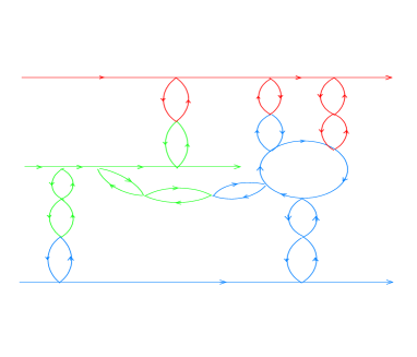
Figure 12: ’t Hooft interactions in the nucleon (left) essentially come to quarks interacting via pion fields (right).

Summing up all interactions of the kind shown in Fig. 12, left, seems to be a hopeless task. Nevertheless, the nucleon binding problem can be solved exactly when two simplifications are used. The first exploits the fact that in the instanton vacuum there are two lightest degrees of freedom: pions (since they are the Goldstone bosons) and quarks with the dynamical mass $M$. All the rest collective excitations of the instanton vacuum are much heavier, and one may wish to neglect them. Pions arise from summing up the $q\bar{q}$ bubbles schematically shown in Fig. 12, left. The resulting effective low-energy theory takes the form of the non-linear $\sigma$-model introduced in section 6:

$${\cal L}_{\rm eff}=\bar{q}\,\left[i\partial\hskip-6.0pt/-M\exp(i\gamma_{5}\pi^{A}\tau^{A}/F_{\pi})\right]\,q.$$ (8.1)

The absence of the explicit kinetic energy term for pions (which would lead to the double counting) distinguishes it from the Manohar–Georgi model [112]. Expanding the exponent to the first power in $\pi^{A}$ we find that the dimensionless pion–constituent quark coupling,

$$g_{\pi qq}=\frac{M}{F_{\pi}}\approx 4,$$ (8.2)

is quite strong. The domain of applicability of the low-energy effective theory (8.1) is restricted by momenta $k<1/\bar{\rho}=600\,{\rm MeV}$, which is the inverse size of constituent quarks. At higher momenta one starts to feel the internal structure of constituent quarks, and the two lightest degrees of freedom of eq. (8.1) become insufficient. However, the expected typical momenta of quarks in the nucleon are of the order of $M\approx 345\;{\rm MeV}$, which is inside the domain of applicability of the low-momentum effective theory.

The chiral interactions of constituent quarks in the nucleon, following from the effective theory (8.1), are schematically shown in Fig. 12, right, where quarks are denoted by lines with arrows. Notice that, since there is no explicit kinetic energy for pions in eq. (8.1), the pion propagates only through quark loops. Quark loops induce also many-quark interactions indicated in Fig. 12 as well. We see that the emerging picture is rather far from a simple one-pion exchange between the constituent quarks: the non-linear effects in the pion field are essential.

The second simplification is achieved in the limit of large $N_{c}$. For $N_{c}$ colours the number of constituent quarks in a baryon is $N_{c}$ and all quark loop contributions are also proportional to $N_{c}$. Therefore, at large $N_{c}$ one can speak about a classical self-consistent pion field inside the nucleon: quantum fluctuations about the classical field are suppressed as $1/N_{c}$. The problem of summing up all diagrams of the type shown in Fig. 12 is thus reduced to finding a classical pion field pulling $N_{c}$ massive quarks together to form a bound state.

9 Chiral Quark–Soliton Model

Let us imagine a classical time-independent pion field which is strong and spatially wide enough to form a bound-state level in the Dirac equation following from eq. (8.1). The background chiral field is colour-neutral, so one can put $N_{c}$ quarks on the same level in an antisymmetric state in colour, i.e. in a colour-singlet state. Thus we obtain a baryon state, as compared to the vacuum.

One has to pay for the creation of this trial pion field, however. Since there are no terms depending directly on the pion field in the low-momentum theory (8.1) the energy of the pion field is actually encoded in the shift of the lower negative-energy Dirac sea of quarks, as compared to the free case with zero pion field. The baryon mass is the sum of the bound-state energy and of the aggregate energy of the lower Dirac sea, see Fig. 13. It is a functional of the trial pion field; one has to minimize it with respect to that field to find the self-consistent pion field that binds quarks inside a baryon. It is a clean-cut problem, and can be solved numerically or, approximately, analytically. The description of baryons based on this construction has been named the Chiral Quark–Soliton Model (CQSM) [113, 114, 115].

Figure 13: The nucleon mass is a sum of the energy of three ‘valence’ quarks $E_{\rm level}$ and of the infinite number of ‘sea’ quarks whose energy is the aggregate energy of the lower Dirac continuum, $E_{\rm field}$. Solid lines are occupied states in the pion background field, each $N_{c}$ times degenerate.

The model reminds the large-$Z$ Thomas–Fermi atom where $N_{c}$ plays the role of $Z$. Fortunately, corrections to the model go as $1/N_{c}$ or even as $1/N_{c}^{2}$ and have been computed for many observables. In the Thomas–Fermi model of atoms corrections to the self-consistent (electric) field are of the order of $1/\sqrt{Z}$ and for that reason are large unless atoms are very heavy.

In the end of the 80’s and the beginning of the 90’s dozens of baryon characteristics have been computed in the CQSM, including masses, magnetic moments, axial constants, formfactors, splittings inside the mutliplets and between multiplets, polarizability, fraction of nucleon spin carried by quarks, etc. – see [116, 79, 117, 118] for reviews and references therein.

Starting from 1996 a new class of problems have been addressed, namely parton distributions in the nucleon at low virtuality [119]. Parton distributions are a snapshot of the nucleon in the infinite momentum frame. One needs an inherently relativistic model in order to describe them consistently. For example, a bag model or any other nonrelativistic model with three quarks in a bound state, being naively boosted to the infinite-momentum frame gives a negative distribution of antiquarks, which is nonsense. On the contrary, being a relativistic field-theoretic model CQSM predicts parton distributions that satisfy all general requirements known in full QCD, like positivity and sum rules constraints.

Numerous parton distributions have been computed in the CQSM, mainly by the Bochum group [119, 120, 121], see also [122, 123, 124] and references therein. There have been a number of mysteries from naive quark models’ point of view: the large number of antiquarks already at a low virtuality, the ‘spin crisis’ [125], the large flavour asymmetry of antiquarks, etc. The CQSM explains all those ‘mysteries’ in a natural way as it incorporates, together with valence quarks bound by the isospin-1 pion field, the negative-energy Dirac sea. Furthermore, the CQSM predicts nontrivial phenomena that have not been observed so far: large flavour asymmetry of the polarized antiquarks [121], transversity distributions [126], peculiar shapes of the so-called skewed parton distributions [127] and other phenomena in hard exclusive reactions [128]. Baryon dynamics is rich and far from naive “three quarks” expectations.

Finally, I would like to stress that physical quantities discussed in this review (and many more remaining beyond) are all expressed, via the ‘transmutation of dimensions’, through the only dimensionful quantity there is in QCD, that is $\Lambda$, as it should be in the ultimate theory. Instantons serve as a bridge from the first principles of QCD – via the microscopic mechanism of spontaneous chiral symmetry breaking – to the observables. Once the basic properties of the instanton vacuum are established one does not need to play with parameter fitting, going from one observable to another. Instantons provide a coherent picture of very different phenomena in strong interactions, and I find it quite remarkable.

I am most grateful to Victor Petrov, Pavel Pobylitsa and Maxim Polyakov for a long-time collaboration on topics presented here.

10 Summary

1. The would-be linear confining potential of the pure glue world is necessarily screened by pion production at very moderate separations between quarks. Therefore, light hadrons need not be sensitive to confinement forces but rather to the dynamics of the spontaneous chiral symmetry breaking (SCSB).

2. Very likely, the SCSB is driven by instantons – large non-perturbative fluctuations of the gluon field having the meaning of tunneling. The SCSB is due to ‘hopping’ of quarks from one randomly situated instanton to another, each time flipping the helicity. The instanton theory of the SCSB is in agreement with the low-energy phenomenology (cf. the chiral condensate $<\bar{\psi}\psi>$, the dynamical quark mass $M(p)$, $F_{\pi}$, $m_{\eta^{\prime}}$…) and seems to be confirmed by direct lattice methods. Furthermore, lattice simulations indicate that instantons alone are responsible for the properties of lightest hadrons $\pi,\rho,N,...$.

3. Instantons induce not only very strong non-perturbative quark interactions but also new and interesting vertices with an additional gluon emission. In particular, they induce a large anomalous chromomagnetic moment which can play an important role in soft high-energy hadron scattering, e.g. in spin phenomena.

4. Summing up instanton-induced quark interactions in baryons leads to the Chiral Quark–Soliton Model where baryons appear to be bound states of constituent quarks pulled together by the chiral field. The model enables one to compute numerous parton distributions, as well as ‘static’ characteristics of baryons – with no fitting parameters whatsoever.

5. For highly excited baryons ($m\!=\!1.5\!-\!3\,{\rm GeV}$) the relative importance of confining forces vs. those of the SCSB may be reversed. One can view a large-spin $J$ resonance as due to a short-time stretch of an unstable string or, alternatively, as a rotating elongated pion cloud [18]. What picture is more adequate is a question to experiment. In the first case the dominant decay is on the average of the type ${\rm Bar}_{J}\to{\rm Bar}_{\sim J/2}+{\rm Mes}_{\sim J/2}$; in the second case it is mainly a cascade ${\rm Bar}_{J}\to{\rm Bar}_{J-1}+\pi\to{\rm Bar}_{J-2}+\pi\pi\to...$ Studying resonances can elucidate the relation between chiral and confining forces.

References

- [1] A. Belavin, A. Polyakov, A. Schwartz and Yu. Tyupkin, Phys. Lett. 59 (1975) 85
- [2] A. Polyakov, Nucl. Phys. B 120 (1977) 429
-
[3]
G. ’t Hooft, Phys. Rev. Lett. 37 (1976) 8;
Phys. Rev. D 14 (1976) 3432; Erratum: ibid. D 18 (1978) 2199 - [4] C. Callan, R. Dashen and D. Gross, Phys. Rev. D 17 (1978) 2717
- [5] E. Shuryak, Nucl. Phys. B 203 (1982) 93, 116, 140
- [6] E.M. Ilgenfritz and M. Müller-Preussker, Nucl. Phys. B184 (1981) 443
- [7] D. Diakonov and V. Petrov, Nucl. Phys. B 245 (1984) 259
- [8] M. Shifman, A. Vainshtein and V. Zakharov, Nucl. Phys. B 147 (1979) 385
- [9] D. Diakonov, The U(1) problem and instantons, in: Gauge Theories of the Eighties, Lecture Notes in Physics, Springer-Verlag (1983) p. 207
- [10] D. Diakonov and V. Petrov, Phys. Lett. B 147 (1984) 351
- [11] D. Diakonov and V. Petrov, Sov. Phys. JETP 62 (1985) 204; Sov. Phys. JETP 62 (1985) 431; Nucl. Phys. B 272 (1986) 457
-
[12]
D. Diakonov and V. Petrov, Spontaneous breaking of chiral symmetry in the instanton
vacuum, preprint LNPI-1153 (1986), in: Hadron matter under extreme
conditions, Kiew (1986) p. 192;
D. Diakonov and V. Petrov, in: Quark Cluster Dynamics, Lecture Notes in Physics, Springer-Verlag (1992) p. 288 - [13] P. Pobylitsa, Phys. Lett. B 226 (1989) 387
- [14] D. Diakonov, V. Petrov and P. Pobylitsa, Phys. Lett. B 226 (1989) 372
- [15] D. Diakonov, in: Skyrmions and Anomalies, World Scientific (1987) p. 27
- [16] G. Bali, K. Schilling and A. Wachter, in: Confinement 95, eds. H. Toki et al., World Scientific (1995) p. 82, hep-lat/9506017
- [17] F. Karsch, E. Laermann and A. Peikert, Nucl. Phys. B605, 579 (2001), hep-lat/0012023
- [18] D. Diakonov and V. Petrov, Rotating chiral solitons lie on linear Regge trajectories, preprint LNPI-1394 (1988); see also D. Diakonov, Acta Phys. Polon. B 25 (1994) 17.
-
[19]
E. Shuryak and J. Verbaarschot, Nucl. Phys. B 410 (1993) 55;
T. Schäfer, E. Shuryak and J. Verbaarschot, Nucl. Phys. B 412 (1994) 143;
T. Schäfer and E. Shuryak, Phys. Rev. D50 (1994) 478 - [20] E. Shuryak, Rev. Mod. Phys. 65 (1993) 1
-
[21]
M.-C. Chu, J. Grandy, S. Huang and J. Negele, Phys. Rev. Lett. 70
(1993) 225; Phys. Rev. D49 (1994) 6039;
J. Negele, Nucl. Phys. Proc. Suppl. 73 (1999) 92, hep-lat/9810053 - [22] T. Schäfer and E. Shuryak, Rev. Mod. Phys. 70 (1998) 323, hep-ph/9610451
- [23] L.D. Faddeev, Looking for multi-dimensional solitons in: Non-local Field Theories, Dubna (1976)
- [24] R. Jackiw and C. Rebbi, Phys. Rev. Lett. 37 (1976) 172
- [25] J.D. Jackson and L.B. Okun, Rev. Mod. Phys. 73 (2001) 663, hep-ph/0012061
- [26] V. Novikov, M. Shifman, A. Vainshtein and V. Zakharov, Nucl. Phys. B 191 (1981) 301
- [27] D. Diakonov, M. Polyakov and C. Weiss, Nucl. Phys. B 461 (1996) 539, hep-ph/9510232
- [28] C. Bernard, Phys. Rev. D 19 (1979) 3013
- [29] A. Hasenfratz and P. Hasenfratz, Nucl. Phys. B 193 (1981) 210
- [30] A. Vainshtein, V. Zakharov, V. Novikov and M. Shifman, Sov. Phys. Uspekhi 136 (1982) 553
- [31] D. Diakonov and M. Polyakov, Nucl. Phys. B 389 (1993) 109
- [32] D. Diakonov and V. Petrov, Phys. Rev. D 50 (1994) 266
-
[33]
V. Fateev, I. Frolov and A. Schwartz, Nucl. Phys. B 154 (1979) 1;
V. Fateev, I. Frolov and A. Schwartz, Sov. J. Nucl. Phys. 30 (4) (1979) 590 - [34] B. Berg and M. Lüscher, Comm. Math. Phys. 69 (1979) 57
- [35] D. Diakonov and M. Maul, Nucl. Phys. B 571 (2000) 91, hep-th/9909078
- [36] P. de Forcrand, M. G. Perez, I.-O. Stamatescu, Nucl. Phys. B 499 (1997) 409, hep-lat/9701012
- [37] T. DeGrand, A. Hasenfratz and T. Kovacs, Nucl. Phys. B 505 (1997) 417, hep-lat/9705009
-
[38]
D. Diakonov and V. Petrov, in: Non-perturbative approaches to Quantum
Chromodynamics, Proc. int. workshop at ECT*, Trento, 1995, ed. D. Diakonov,
Gatchina (1995) p. 239;
D. Diakonov and V. Petrov, Phys. Scripta 61 (2000) 536, hep-lat/9810037 - [39] V. de Alfaro, S. Fubini and G. Furlan, Phys. Lett. B 65 (1976) 163
- [40] C. Callan, R. Dashen and D. Gross, Phys. Rev. D 19 (1979) 1826
- [41] T.C. Kraan and P. van Baal, Phys. Lett B 428 (1998) 268, hep-th/9802049; Nucl. Phys. B 533 (1998) 627, hep-th/9805168
- [42] K. Lee and C. Lu, Phys. Rev. D 58 (1998) 025011, hep-th/9802108
- [43] E.B. Bogomolnyi, Yad. Fiz. 24 (1976) 861 [Sov. J. Nucl. Phys 24 (1976) 449]
- [44] M.K. Prasad and C.M. Sommerfeld, Phys. Rev. Lett. 35 (1975) 760
- [45] G. H͡ooft, Nucl. Phys. B 138 (1978) 1
- [46] G. Mack, Cargèse lectures (1979)
- [47] A. Montero, J. Negele, Phys. Lett. B 533 (2002) 322, hep-lat/0202023
- [48] K. Lee and P. Yi, Phys. Rev D 56 (1997), hep-th/9702107
- [49] D. Diakonov and V. Petrov, hep-th/0212018
- [50] N.M. Davies, T.J. Hollowood and V.V. Khoze, hep-th/0006011
- [51] K. Zarembo, Nucl. Phys. B 463 (1996) 73, hep-th/9510031
- [52] D.J. Gross, R.D. Pisarski and L.G. Yaffe, Rev. Mod. Phys. 53 (1981) 43
- [53] N. Weiss, Phys. Rev. D 24 (1981) 475; Phys. Rev. D 25 (1982) 2667
- [54] B.J. Harrington and H.K. Shepard, Phys. Rev. D 17 (1978) 2122; Phys. Rev. D 18 (1978) 2990
- [55] D. Diakonov and A. Mirlin, Phys. Lett. B 203 (1988) 299
- [56] N.M. Davies, T.J. Hollowood, V.V. Khoze and M.P. Mattis, Nucl. Phys. B 559 (1999) 123, hep-th/9905015
- [57] V.A. Novikov, M.A. Shifman, A.I. Vainshtein and V.I. Zakharov, Nucl. Phys. B 229 (1983), 394, 407
- [58] E.M. Ilgenfritz, B.V. Martemyanov, M. Muller-Preussker, S. Shcheredin and A.I. Veselov, Phys. Rev. D 66 (2002) 074503, hep-lat/0206004
- [59] C. Gattringer, hep-lat/0210001; C. Gattringer and S. Schaefer, hep-lat/0212029
-
[60]
A. Gonzalez-Arroyo, in: Advanced school on non-perturbative
quantum field physics, M. Asorey and A. Dobado, eds., World Scientific (1998) p. 57,
hep-th/9807108;
A. Gonzalez-Arroyo, A. Montero, Phys.Lett. B 442 (1998) 273, hep-th/9809037;
M. Garcia Perez, A. Gonzalez-Arroyo, A. Montero, C. Pena and P. van Baal, Nucl. Phys. Proc. Suppl. (2000) 83. hep-lat/9909112 - [61] J. Greensite, submitted to Prog. Part. Nucl. Phys., hep-lat/0301023
- [62] D. Diakonov, Mod. Phys. Lett. A 14 (1999) 1909, hep-th/9908069
- [63] D. Diakonov and M. Maul, Phys. Rev. D 66 (2002) 096004, hep-lat/0204012
- [64] M. Bordag, hep-th/0211080
- [65] B. Lucini and M. Teper, JHEP 06 (2001) 050, hep-lat/0103027; Phys. Rev. D 64 (2001) 105019, hep-lat/0107007
- [66] L. Del Debbio, H. Panagopoulos, P. Rossi and E. Vicari, JHEP 01 (2002) 009, hep-th/0111090
- [67] L. Del Debbio and D. Diakonov, Phys. Lett. B 544 (2002) 202, hep-lat/0205015
- [68] T. Schafer, Phys. Rev. D 66 (2002) 076009, hep-ph/0206062, hep-ph/0204026
- [69] D. Diakonov, invited talk at the 5th International Conference on Quark Confinement and the Hadron Spectrum, Gargnano, Italy, Sep 2002, hep-th/0212187
- [70] T. Banks and A. Casher, Nucl. Phys. B 169 (1980) 103
- [71] D. Diakonov, Habilitation thesis (LNPI, 1986) (unpublished); in: Selected Topics in Nonperturbative QCD, A. Di Giacomo and D. Diakonov, eds., IOS Press (1996) p.397, hep-ph/9602375
- [72] R.A. Janik, M.A. Nowak, G. Papp, and I. Zahed, Phys. Rev. Lett. 81 (1998) 264
- [73] J.C. Osborn, D. Toublan and J.J. Verbaarschot, Nucl. Phys. B 540 (1999) 317
- [74] M. Nowak, hep-ph/0112296
- [75] J. Negele, Nucl. Phys. Proc. Suppl. 73 (1999) 92, hep-lat/9810053
-
[76]
T. DeGrand and A. Hasenfratz,
Phys. Rev. D 64 (2001) 034512, hep-lat/0012021;
M. Göckeler, P. Rakow, S. Schaefer, A. Schäfer, Nucl. Phys. B 617 (2001) 101, hep-lat/0107016;
T. Blum et al., Phys. Rev. D 65 (2002) 014504, hep-lat/0105006;
R. G. Edwards and U. M. Heller, Phys. Rev. D 65 (2002) 014505, hep-lat/0105004;
T. Lippert, H. Neff, K. Schilling and W. Schroers, Phys. Rev. D 65 (2002) 014506, hep-lat/0105001;
C. Gattringer, Phys. Rev. Lett. 88 (2002) 221601, hep-lat/0202002 - [77] I. Horváth et al., Phys. Rev. D 66 (2002) 034501, hep-lat/0201008
- [78] P. Bowman, U. Heller, D. Leinweber and A. Williams, submitted to 20th International Symposium on Lattice Field Theory (LATTICE 2002), hep-lat/0209129
- [79] D. Diakonov, in: Advanced School on Non-perturbative Quantum Field Theory, M. Asorey and A. Dobado, eds., World Scientific (1998) p. 1, hep-th/9802298
- [80] E. Witten, Nucl. Phys. B 156 (1979) 269
- [81] G. Veneziano, Nucl. Phys. B 159 (1979) 231
- [82] M. Nowak, J. Verbaarschot and I. Zahed, Nucl. Phys. B 324 (1989) 1
- [83] H. Leutwyler and A. Smilga, Phys. Rev. D 46 (1992) 5607
- [84] D. Diakonov and M. Eides, Zh. Eksp. Teor. Fiz. 81 (1981) 434 [Sov. Phys. JETP 54 (1981) 232
- [85] Y. Nambu and G. Jona-Lasinio, Phys. Rev. 122 (1961) 345; 124 (1961) 246
- [86] M. Musakhanov, Nucl. Phys. A 699 (2002) 340, hep-ph/0206233
- [87] R.G. Betman and L.V. Laperashvili, Sov. J. Nucl. Phys. 41 (1985) 295
- [88] D. Diakonov, H. Forkel and M. Lutz, Phys. Lett. B 373 (1996) 147, hep-ph/9512385
- [89] R. Rapp, T. Schäfer, E. Shuryak and M. Velkovsky, Phys. Rev. Lett. 81 (1998) 53, hep-ph/9711396
- [90] M. Alford, K. Rajagopal and F. Wilczek, Phys. Lett. B 422 (1998) 247, hep-ph/9711395
- [91] G. Carter and D. Diakonov, Nucl. Phys. A 642 (1998) 78; Phys. Rev. D 60 (1999) 016004, hep-ph/9812445
- [92] G. Carter and D. Diakonov, Nucl. Phys. B 582 (2000) 571, hep-ph/0001318
-
[93]
E.M. Levin and L.L. Frankfurt, JETP Lett. 2 (1965) 65;
H.J. Lipkin and F. Scheck, Phys. Rev. Lett. 16 (1966) 71;
V.V. Anisovich and V.M. Shekhter, Nucl. Phys. B 55 (1973) 455 - [94] See e.g. V.V. Anisovich, M.N.Kobrinsky, J. Nyiri and Yu.M. Shabelski, Quark Model and High Energy Collisions, World Scientific (1985), and references therein
-
[95]
For a review see, L.G. Pondrom, Phys. Rept.
122 (1985) 57;
J. Lach, Hyperon polarization: an experimental overview, FERMILAB-CONF-92-378 -
[96]
F.E. Low, Phys. Rev. D 12 (1975) 163;
S. Nussinov, Phys. Rev. Lett. 37 (1975) 1286 -
[97]
E.A. Kuraev, L.N. Lipatov and V.S. Fadin, Sov. Phys. JETP 45 (1978)
199;
Ya.Ya. Balitsky and L.N. Lipatov, Sov. J. Nucl. Phys. 28 (1978) 22 - [98] S. Donnachie, G. Dosch, O. Nachtmann and P. Landshoff, Pomeron physics and QCD, Cambridge Univ. Pr. (2002) 347 p.
-
[99]
O. Nachtmann, Ann. Phys. (NY) 209 (1991) 436;
H. -G. Dosch, E. Ferreira and A. Kramer, Phys. Lett. B 289 (1992) 153. - [100] J. Soffer, in: Batavia 1999, Hyperon Physics, p.121-126, hep-ph/9911373
-
[101]
A. Ringwald, Nucl. Phys. B 330 (1990) 1;
O. Espinosa, Nucl. Phys. B 343 (1990) 310;
L. McLerran, A. Vainshtein and M. Voloshin, Phys. Rev. D 42 (1990) 171,180;
V. Zakharov, Nucl. Phys. B 353 (1991) 683;
A. Mueller, Nucl. Phys. B 381 (1992) 597 - [102] N.I. Kochelev, Phys. Lett. B 426 (1998) 149; see also hep-ph/9707418
- [103] J. Balla, M. Polyakov and C. Weiss, Nucl. Phys. B 510 (1998) 327
-
[104]
E. Shuryak, Phys. Lett. B 486 (2000) 378;
D. Kharzeev, Yu. Kovchegov and E. Levin, Nucl. Phys. A 690 (2001) 621;
M. Nowak, E. Shuryak and I. Zahed, Phys. Rev. D 64 (2001) 034008 - [105] E. Shuryak, hep-ph/0205031
- [106] L.S. Brown, R.D. Carlitz, D.B. Creamer and C. Lee, Phys. Rev. D 17 (1978) 1583
- [107] F. Schrempp, J. Phys. G 28 (2002) 915, hep-ph/0109032
- [108] F. Schrempp and A. Utermann, Phys. Lett. B 543 (2002) 197, hep-ph/0207300
-
[109]
I. Balitsky and V. Braun, Phys. Lett. B 314 (1993) 237; Phys. Rev. D 47 (1993)
1879;
A. Ringwald and F. Schrempp, in: Quarks ’94, Proc. 8th Int. Seminar, Vladimir, Russia, 1994, ed. D. Grigoriev et al., World Scientific (1995) p. 170;
S. Moch, A. Ringwald and F. Schrempp, Nucl. Phys. B 507 (1997) 134, hep-ph/9609445;
A. Ringwald and F. Schrempp, Phys. Lett. B 438 (1998) 217, hep-ph/9806528;
A. Ringwald and F. Schrempp, Phys. Lett. B 503 (2001) 331, hep-ph/0012241 - [110] C. Adloff et al., Eur. Phys. J. C 25 (2002) 495, hep-ex 0205078
- [111] K.F. Liu et al., Phys. Rev. D 59 (1999) 112001, hep-ph/9806491
- [112] A. Manohar and H. Georgi, Nucl. Phys. B 234 (1984) 189
-
[113]
S. Kahana, G. Ripka and V. Soni, Nucl. Phys. A 415 (1984) 351;
S. Kahana and G. Ripka, Nucl. Phys. A 429 (1984) 462 - [114] M.S. Birse and M.K. Banerjee, Phys. Lett. B 136 (1984) 284
-
[115]
D. Diakonov and V. Petrov, Sov. Phys. JETP Lett. 43 (1986) 57;
D. Diakonov, V. Petrov and P. Pobylitsa, in: Proc. 21st PNPI Winter School, Leningrad (1986) p. 158; Nucl. Phys. B 306 (1988) 809 - [116] C. Christov et al., Prog. Part. Nucl. Phys. 37 (1996) 91, hep-ph/9604441
- [117] G. Ripka, Quarks bound by chiral fields, Clarendon Press, Oxford (1997), 222 p.
- [118] D. Diakonov and V. Petrov, in: At the Frontiers of Particle Physics (Handbook of QCD), ed. M. Shifman, World Scientific (2001) vol.1 p. 359, hep-ph/0009006
- [119] D. Diakonov, V. Petrov, P. Pobylitsa, M. Polyakov and C. Weiss, Nucl. Phys. B 480 (1996) 341, hep-ph/9606314; Phys. Rev. D 56 (1997) 4069, hep-ph/9703420
- [120] P. Pobylitsa, M. Polyakov, K. Goeke, T. Watabe and C. Weiss, Phys. Rev. D 59 (1999) 034024, hep-ph/9804436
- [121] B. Dressler, K. Goeke, M. Polyakov and C. Weiss, Eur. Phys. J. C 14 (2000) 147, hep-ph/9909541
- [122] H. Weigel, L. Gamberg, H. Reinhardt and O. Schroeder, Nucl. Phys. Proc. Suppl. (1999) 74, hep-ph/9807506
- [123] E. Ruiz Arriola, in: Hadrons as solitons, Bled (1999) p. 5, hep-ph/9910382
- [124] M. Wakamatsu, hep-ph/0209011, hep-ph/0212356
- [125] M. Wakamatsu and H. Yoshiki, Nucl. Phys. A 524 (1991) 561
- [126] P. Pobylitsa and M. Polyakov, Phys. Lett. B 389 (1996) 350, hep-ph/9608434
- [127] V. Petrov, P. Pobylitsa, M. Polyakov, I. Börnig, K. Goeke and C. Weiss, Phys. Rev. D 57 (1998) 4325, hep-ph/9710270
- [128] K. Goeke, M. Polyakov and M. Vanderhaeghen, Prog. Part. Nucl. Phys. 47 (2001) 401, hep-ph/0106012