Front cover: The Hermetic Truth of Hadrons by Anders Sandberg, inspired by M.C. Escher’s last drawing, Snakes (1969). Printed with the permission of the author.

This is a version of my PhD thesis (defended on Oct 4th, 2002) prepared for submission to the arXiv. It is almost identical to the official copy. However, to comply with the arXiv requirements some changes had to be done, resulting in a few differences and layout mistakes. A more faithful version of the thesis can be found at the web address http://www.nat.vu.nl/ bacchett/research/thesis.pdf.

The work described in this thesis is part of the research programme of the Stichting voor Fundamenteel Onderzoek der Materie (FOM), which is financially supported by the Nederlandse Organisatie voor Wetenschappelijk Onderzoek (NWO).

promotor: prof.dr. P.J.G. Mulders

Contents

toc

Notations and conventions

The conventions will mainly follow the book of Peskin and Schroeder [147]. We use the metric tensor

$$g^{\mspace{2.0mu}\mu\nu}=\begin{pmatrix}1&0&0&0\\ 0&-1&0&0\\ 0&0&-1&0\\ 0&0&0&-1\end{pmatrix},$$

with Greek indices running over 0,1,2,3. Repeated indices are summed in all cases. Light italic roman type will be used for four-vectors, while boldface italic will be used for three-vectors.

Light-cone vectors

Light-cone vectors will be indicated as

$$a^{\mspace{2.0mu}\mu}=\left[a^{-},\;a^{+},\;\bm{a}_{T}\right]=\left[\frac{a^{0}-a^{3}}{\sqrt{2}},\;\frac{a^{0}+a^{3}}{\sqrt{2}},\;a^{1},\;a^{2}\right].$$

The dot-product in light-cone components is

$$\begin{split}a\cdot b&=a^{+}b^{-}+b^{-}a^{+}-\bm{a}_{T}\cdot\bm{b}_{T}\\ &=a^{+}b^{-}+b^{-}a^{+}-a^{i}b^{i}\\ &=a^{+}b^{-}+b^{-}a^{+}-a_{x}b_{x}-a_{y}b_{y}\end{split}$$

The two-dimensional transverse parts of the vectors will be written in boldface with an index $T$ and Latin indices will be used to denote the two transverse components only. Note that

$$\bm{a}_{T} =(a_{x},\;a_{y}), a_{T}^{\mspace{2.0mu}\mu} =[0,\;0,\;\bm{a}_{T}], a_{T\mu} =[0,\;0,\;-\bm{a}_{T}].$$

We introduce the projector on the transverse subspace

$$g_{T}^{\mspace{2.0mu}\mu\nu}=\begin{pmatrix}0&0&0&0\\ 0&-1&0&0\\ 0&0&-1&0\\ 0&0&0&0\end{pmatrix},$$

We define the antisymmetric tensor so that

$$\epsilon^{0123} =+1, \epsilon_{\mspace{2.0mu}0123} =-1.$$

and we define the transverse part of the antisymmetric tensor as

$$\epsilon_{T}^{\mspace{2.0mu}\mu\nu}=\epsilon^{-+\mu\nu}=\epsilon^{03\mu\nu}.$$

Dirac matrices

Dirac matrices will be often expressed in the chiral or Weyl representation, i.e.

$$\gamma^{0} =\begin{pmatrix}0&\bm{1}\\ \bm{1}&0\end{pmatrix}, \gamma^{i} =\begin{pmatrix}0&-\bm{\sigma}^{i}\\ \bm{\sigma}^{i}&0\end{pmatrix}, \gamma_{5} =\begin{pmatrix}\bm{1}&0\\ 0&-\bm{1}\end{pmatrix},$$

and we will make use of the Dirac structure

$$\sigma^{\mspace{2.0mu}\mu\nu}\equiv\frac{{\rm i}}{2}\left[\gamma^{\mspace{2.0mu}\mu},\gamma^{\nu}\right].$$

Chapter 1 Introduction

In this thesis I will discuss three different ways to observe the transverse spin of quarks inside the nucleons. Before embarking on such an undertaking, I would like to spend a few pages on explaining what makes this problem so interesting to justify investing years of research on it. This introduction is meant especially for nonexperts, since I will review notions well known to the experts in the field.

1.1 The structure of matter

When we talk about quarks inside nucleons we are referring to the best paradigm we currently have to describe the elementary structure of matter. The comprehension of this elementary structure is a question that has allured philosophers and scientists since the historical origins of philosophical thought. It is striking to observe that as early as six hundred years BC, Greek philosophers were already wondering: are there fundamental elements in nature, what are they and how do they interact? Today, after more than two millennia, we learned a lot about the structure of matter, but some of the most important questions still elude our comprehension. We are still engaged in one of the oldest quests of human mind.

Since 1803, when Dalton suggested his atomic hypothesis [85], we have gradually realized that almost all matter on earth is made up of atoms. Atoms contain electrons – identified for the first time by J. J. Thomson in 1897 [166, 167] – and nuclei – introduced for the first time by E. Rutherford in 1911 [153, 98]. The efforts to explain precisely the structure of atoms and the electromagnetic interaction binding together electrons and nuclei lead to two of the major achievements of physics in the last century: Quantum Mechanics and Quantum Electrodynamics (QED).

In the meantime, more investigations were carried out to grasp the structure of the nucleus inside atoms. The smallest known nucleus was identified with a single particle [154], the proton, while a second constituent of heavier nuclei, the neutron, was eventually observed by J. Chadwick [75]. Since they are the constituents of the nucleus, protons and neutrons are referred to as nucleons. They are kept together by the nuclear force, of which at the moment we have only an incomplete understanding.

Although the electrons are responsible for the chemical properties of atoms, they account for a very small fraction of the mass of the atom. The mass of an electron is about 0.511 MeV, while the mass of a proton is about 938 MeV. Therefore, nucleons make up for more than 99.9% of ordinary atomic matter. If we want to understand matter, we cannot set aside the problem of explaining the structure of nucleons. Nucleons belong to the more general class of hadrons, of which they are the most abundant specimen. At first, hadrons were classified as elementary particles, i.e. without any internal substructure. Very soon this appeared to be an unsatisfactory hypothesis, in particular since there are so many of them (several dozens). Nowadays, the study of the structure of hadrons represents a field of research on its own, often designated with the name of hadronic physics. An up-to-date review of the field can be found in Refs. 48 and 74.

1.2 Hadrons and deep inelastic scattering

To interpret the information available on the properties of hadrons in 1964, M. Gell-Mann [99] and G. Zweig [172] independently suggested that hadrons are composed of smaller constituents, the quarks, having spin $1/2$, a fractional electric charge and a new degree of freedom, called flavor. This model is often referred to as constituent quark model. Gell-Mann himself seemed not to believe in the existence of quarks as real entities, but rather regarded them as convenient concepts [99]. One of the reasons to be skeptical about the real existence of quarks was that they have a charge that is just a fraction of the electron charge, while the charge of all other elementary particles is an integer multiple of that.

The quark model aimed at describing the mass, charge and spin of the hadrons. For instance, the proton has a mass of about 1 GeV, a charge $+e$ (the same as the electron, but with opposite sign) and spin equal to $1/2$. According to the model, a proton with its spin, for instance, in the up direction is made of two quarks with flavor up and charge $2e/3$ plus one quark with flavor down and charge $-e/3$. Two of the quarks have spin $1/2$ in the up direction and one has spin $1/2$ in the down direction. Each of the three quarks carries about one-third of the mass of the proton.

Looking at the “extrinsic” properties of hadrons – like their mass, charge and spin – was not enough to unravel the details of their structure. To glance at the inside of hadrons, physicists resorted to deep inelastic scattering (DIS) experiments, as in the pioneering experiments led by Friedman, Kendall and Taylor at the Stanford Linear Accelerator Center (SLAC) [49, 66]. In scattering experiments, a focused beam of particles is dispersed by the interaction with a target. The way this dispersion takes place yields information on the structure of the target. For instance, the existence of the nucleus was suggested by Rutherford as an explanation to the scattering experiments of Geiger and Marsden [98].

Basically, particle accelerators as the one at SLAC are exploited as microscopes of extremely high resolution. The experiments at SLAC scattered electrons off hydrogen. The interaction proceeds via the exchange of a virtual photon with high energy and momentum. A measure of the resolution of the experiment is given by the four-momentum squared of the virtual photon, $Q^{2}$, or rather by the associated wavelength $\hslash/Q$. The SLAC experiments reached a maximum $Q^{2}$ of 7.4 GeV², corresponding to a resolution of the order of $1/10$ of the proton size.

The results of the SLAC experiments indicated that the scattering data did not exhibit a (strong) dependence on $Q^{2}$. They depended rather on the variable that was later to be named $x$-Bjorken, $x_{B}$, in honor of J. Bjorken. This property, called scaling, was predicted by Bjorken himself [46] and explained by R. Feynman [95, 47], who introduced the parton model: the proton was pictured to be a collection of almost free point-like constituents off which the electrons scatter incoherently. The constituents of the proton were initially called partons, but it soon became clear that they had a lot in common with the quarks of Gell-Mann and Zweig.

Feynman’s partons have spin $1/2$, fractional electric charge and flavor, but they have a very small mass compared to Gell-Mann’s quarks, a few MeV against about 300 MeV. Consequently, we call them current quarks, to distinguish them from the constituent quarks of the quark model. But this is not the only difference between the two models. In the constituent quark model, the proton is made up just of three quarks, while in the parton model it turns out that there is a huge number of quark-antiquark pairs, together with a huge number of electrically neutral particles, later to be identified as gluons.

Deep inelastic scattering experiments are performed in some of the world’s largest experimental facilities for high energy physics, such as CERN, SLAC, DESY, BNL. They usually employ beams of electrons, positrons, muons or, more rarely, neutrinos. They scatter off different kinds of fixed targets or off a beam of protons, and they operate at different energies and kinematic coverage.

1.3 Quantum Chromodynamics and confinement

The parton model raised a profound question. We experience that matter, at least in the normal conditions on earth, is composed of hadrons – it is the so-called hadronic matter. If quarks are the hypothetical constituents of hadrons, they must be bound extremely tight to explain why we have never directly observed a single isolated quark, nor a different state of matter other than hadronic. This essential feature of quark dynamics is known as confinement. Yet, deep inelastic scattering suggests that in the interaction with a high-$Q^{2}$ virtual photon, quarks behave as if they were essentially free. This property is known as asymptotic freedom. The question is then: how is it possible to devise a theory to reconcile these two opposing properties, confinement and asymptotic freedom?

A first attempt to implement confinement was done by postulating that quarks have a color charge and that all detectable objects have to be colorless (cf. Refs. 142, 143 and references therein). By virtue of this assumption, it is impossible to see an isolated, colored quark. On the other hand, such a point of view is not suited to describe asymptotic freedom. There was the need of a theory that could describe the binding of colored quarks as a dynamical mechanism.

To shape a new theory of color interactions, it seemed natural to follow the example of Quantum Electrodynamics, the quantum field theory of electromagnetic interactions. QED is in essence a perturbative theory, which works because electromagnetic interactions are weak. In fact, electrons can be separated quite easily from atoms and observed as free particles. A measure of the strength of the electromagnetic interaction is given by the value of the electromagnetic coupling constant $\alpha\approx 1/137$. From renormalization of QED, it is known that in reality $\alpha$ is not constant, but it has to increase as the momentum exchange of the interaction increases, or equivalently as the interaction takes place over shorter distances. However, the increase of the coupling is so weak (e.g. $\alpha\approx 1/135$ at $Q^{2}=1000$ GeV²) that perturbative QED works brilliantly for any electrodynamics experiment we might do. Fig. 1.1 shows approximately the way the electromagnetic coupling constant changes with $Q^{2}$.

Figure 1.1: The running of the electromagnetic coupling constant. The gray area roughly indicates where perturbation theory is not trustworthy anymore. Note the huge scales necessary to achieve a appreciable increase of the coupling.

A breakthrough in the comprehension of quark interactions came in 1973, when D. Gross and F. Wilczek [102, 101] and D. Politzer [149] showed that non-Abelian quantum field theories can display the crucial properties of asymptotic freedom, i.e. the interaction they describe is weak at high momentum transfer (or long distances). This discovery prompted the birth of Quantum Chromodynamics (QCD), a non-Abelian field theory of color interactions.

The difference between QED and QCD can be likened to the difference between the attraction forces of two opposite magnetic poles and of two ends of a spring. In the first case, we know that increasing the distance between the magnets, the attraction diminishes, while, in the second case, separating the two ends the force will increase more and more.

In field theory language, the electromagnetic coupling constant is reduced at large distances due to the effect of vacuum polarization, which is responsible for a screening of the bare electric charge. On the contrary, the color coupling constant is reduced at short distances because the vacuum polarization induces an antiscreening of the charge, or equivalently an enhancement of the charge at large distances. The reason for this different behavior is that gluons, the mediator of the color interaction, carry color charge themselves, while photons, the mediator of the electromagnetic interaction, are chargeless. Ref. 147 (p. 541) and Ref. 96 (p. 5) present enlightening discussions on antiscreening and asymptotic freedom.

Figure 1.2: The running of the strong coupling constant. The gray area roughly indicates where perturbation theory is not trustworthy anymore.

QCD is able to justify asymptotic freedom, but what about confinement? At the moment, we know that QCD is not in contradiction with confinement and might in fact explain it, but we are not able to demonstrate this statement. As in the case of QED, the strength of color interaction is measured by the strong coupling constant $\alpha_{s}$, which has a value of about 0.117 at $Q^{2}=8.3\times 10^{3}$ GeV². But at lower energy scales, e.g. $Q^{2}\approx 1$ GeV², the coupling constant grows and becomes of the order of 1. The running of the strong coupling constant is illustrated in Fig. 1.2. We might deduce that the increase of the coupling constant is a sign of the onset of confinement. In reality, we can only conclude that at low energies we enter a regime where perturbation theory cannot be trusted. Therefore, even if QCD is in principle a consistent theory at any energy scale, we cannot use standard techniques to draw conclusions about its behavior in the nonperturbative regime. To a certain extent, we cannot be sure that QCD is the correct theory in this regime: maybe it is simply an asymptotic approximation of a more profound theory.

In practice, we have to make a distinction between two major branches of QCD: perturbative and nonperturbative, or short-distance and long-distance. Perturbative QCD is relatively well understood. It is essentially similar to QED, it is based on Feynman-diagram approach, although it often requires larger sets of diagrams to attain the desired accuracy. The theory contains pointlike and almost massless fermions (the so-called current quarks) and massless bosons to carry their interactions (the gluons). Probably one of the most important achievements of perturbative QCD is the study of the way deep inelastic scattering data change with $Q^{2}$. The striking agreement between theory and experiments is shown in Fig. 1.3.

Figure 1.3: One of the greatest achievements of perturbative QCD: world data on the $Q^{2}$ dependence of the unpolarized structure function $F_{2}$, compared to theoretical expectations (solid curves) [138].

On the other hand, nonperturbative QCD is poorly understood and it is a challenging playground for fundamental physics. At the moment, our understanding of this theory relies on lattice calculations, effective chiral field theories, and phenomenological models.

We know that nonperturbative QCD should display confinement as a fundamental property, at least under normal conditions. Lattice calculations already provide strong evidence that the quark-quark interaction potential increases linearly, and is therefore a confining potential [39]. It is essential to understand from first principles why this occurs, and it is desirable to explore how it is possible to achieve a deconfined phase of QCD, maybe under extreme conditions (e.g. neutron stars). We also know that in QCD chiral symmetry is approximately valid. On the other hand, the existence of pions, which are nearly massless, suggests that chiral symmetry should be spontaneously broken, with pions being Goldstone bosons. Nonperturbative QCD should be able to explain this feature. Nonperturbative QCD should also explain the transition between massless current quarks and constituent quarks.

Finally and more generally, nonperturbative QCD should lead to a reliable quantitative description of the structure of hadrons and of hadronic phenomena. The question at the heart of hadronic physics is: what is the structure of hadrons in terms of their quark and gluon constituents? Therefore, we might define hadronic physics as the branch of physics that deals with understanding QCD, and in particular nonperturbative QCD.

1.4 Spin physics and the transversity distribution

One of the key questions in understanding the structure of hadrons is: where does the spin of the nucleons come from? In the constituent quark model, the spin of the quarks adds up to yield the total spin of the proton. Deep inelastic scattering experiments, however, show the importance of other contributions, such as the spin of the gluons and the orbital angular momenta of quarks and gluons. A measure of the quark spin contribution is given by the distribution function $g_{1}$, often denoted as $\Delta q$ and usually called the helicity distribution. In a frame of reference where the hadron is moving with a very large speed (infinite momentum frame) and if the direction of its spin is longitudinal to its motion, the helicity distribution describes the number of quarks with their spin aligned with that of the hadron minus the number of quarks with opposite spin, it is therefore a measure of the longitudinal spin of the quarks in the hadron. The quark helicity distribution has been measured with a good precision, as shown in Fig. 1.4. Naively, if the spin of the hadron is entirely due to the quark spin as in the constituent quark model, we expect to have a net balance of one quark spinning in the direction of the proton and thus accounting for the whole proton spin. In reality, it turns out that (the integral of) the helicity distribution accounts for only about 30% of the proton spin! We expect thus that the missing spin is provided by the gluon spin and by the orbital angular momentum of quarks and gluons. These two quantities have not been measured yet. Even worse, we don’t know if it is possible to measure the orbital angular momentum directly [123, 103, 43].

Figure 1.4: The helicity distribution of the proton, $g_{1}$ as a function of the fractional momentum $x$ carried by quarks [9].

Tab. 1.1 shows a list of all polarized deep inelastic scattering experiments, together with their typical energies and the characteristics of their beams and targets. The kinematic coverage of each experiment is indicated in the table by its average $Q^{2}$ (GeV²) and $x_{B}$ range. Columns $P_{B}$ and $P_{T}$ give the average or typical beam and target polarizations as quoted by each experimental group. The column labeled $\mathcal{L}$ is an estimate of the total nucleon luminosity (# of nucleons/cm² times # of beam particles/s) in units of $10^{32}$ nucleons/cm²/s for each experiment.

Table 1.1: Summary of polarized deep inelastic measurements [97].

Lab	Exp.	Year	Beam	$\langle Q^{2}\rangle$	$x_{B}$	$P_{B}$	Target	$P_{T}$	$\mathcal{L}$
SLAC	E80	75	10-16 GeV $e^{-}$	2	0.1 – 0.5	85%	H-butanol	50%	400
	E130	80	16-23 GeV $e^{-}$	5	0.1 – 0.6	81%	H-butanol	58%	400
	E142	92	19-26 GeV $e^{-}$	2	0.03 – 0.6	39%	3He	35%	2000
	E143	93	10-29 GeV $e^{-}$	3	0.03 – 0.8	85%	NH3	70%	1000
							ND3	25%	1000
	E154	95	48 GeV $e^{-}$	5	0.01 – 0.7	82%	3He	38%	3000
	E155	97	48 GeV $e^{-}$	5	0.01 – 0.9	81%	NH3	90%	1000
							LiD	22%	1000
	E155’	99	30 GeV $e^{-}$	3	0.02 – 0.9	83%	NH3	75%	1000
							LiD	22%	1000
CERN	EMC	85	100-200 GeV $\mu^{+}$	11	0.01 – 0.7	79%	NH3	78%	0.3
	SMC	92	100 GeV $\mu^{+}$	4.6	0.006 – 0.6	82%	D-butanol	35%	0.3
		93	190 GeV $\mu^{+}$	10	0.003 – 0.7	80%	H-butanol	86%	0.6
		94-95				81%	D-butanol	50%	0.6
		96				77%	NH3	89%	0.6
DESY	HERMES	95	28 GeV $e^{+}$	2.5	0.02 – 0.6	55%	3He	46%	1
		96-97				55%	H	88%	0.1
		98	28 GeV $e^{-}$			55%	D	85%	0.2
		99-00	28 GeV $e^{+}$			55%	D	85%	0.2
		01-?	28 GeV $e^{-}$			55%	H	85%∗	0.2
CERN	COMPASS	01-?	190 GeV $\mu^{+}$	10	0.005 – 0.6	80%	NH3	90%	3
							LiD	40%	3
BNL	RHIC	02-?	200 GeV $p-p$	$\sim 100$	0.05 – 0.6	70%	Collider	70%	2
DESY	ZEUS/H1	02-?	$28\times 800$ GeV $e-p$	22	0.00006 – 0.6	50%	Collider		0.2

^∗ Transversely polarized target

So far we talked about the longitudinal spin of the quarks inside the proton, but what about the transverse spin? The observable we have to take into consideration is the transversity distribution. In the infinite momentum frame with the proton spin transverse to the direction of motion, the transversity distribution describes the number of quarks with their spin aligned with that of the hadron minus the number of quarks with opposite spin, it is therefore a measure of the transverse spin of the quarks in the hadron. The transversity distribution looks very similar to the helicity distribution, as at first sight they seem related by rotational symmetry. However, we cannot forget the fact that the interpretation of helicity and transversity holds true only in the infinite momentum frame, where the direction of motion of the hadron breaks rotational symmetry.

In the rest frame of the proton, there is a probability to find quark spins aligned with the proton’s spin. This probability is obviously the same no matter what the spin orientation is. If we now boost the proton to a large speed in the direction of its spin, the alignment probability will correspond to the helicity distribution. If we boost the proton in a direction transverse to its spin, the alignment probability will correspond to the transversity distribution. In a nonrelativistic situation, Galilean boosts will not affect the spin distribution and we would still expect helicity and transversity to be equal to each other and to the spin distribution in the rest frame. But in a relativistic context, Lorentz boosts can affect the spin distribution and can cause helicity and transversity to be different from each other and from the rest-frame distribution. The way this difference arises depends on the inner structure of the nucleon.

The transverse spin of quarks is thus another missing piece in the proton spin puzzle. It can give new information on the dynamics of quarks inside hadrons, complementary to the helicity distribution. In spite of this, the transversity distribution escaped notice until 1979, when it was introduced by J. Ralston and D. Soper [151]. In the last decade, it has been evaluated in models [116, 120, 148, 40] and lattice computations [24]. At this point, an experimental measurement will be needed to put all these calculations on test, but unfortunately the transversity distribution is an elusive object to measure. Today, looking for a practical way to observe transversity is still an open problem. Experimental collaborations are planning its measurement at last [105, 83, 73], and some of them will resort to the methods discussed in this thesis.

1.5 Outline of the thesis

The goal of the thesis is to discuss three different ways to observe the quark transversity distribution in deep inelastic scattering.

To start with, in chapter 2 I will review the formalism of deep inelastic scattering. I will introduce the parton distribution functions and I will devote a particular attention to the transversity distribution function. I will discuss totally inclusive DIS, where only the scattered electron is detected, and I will show that it is not possible to measure the transversity distribution in this kind of process.

In chapter 3, I will turn the attention to one-particle inclusive DIS, where one of the outgoing hadrons is detected in coincidence with the scattered electron. I will introduce fragmentation functions to describe the production of hadronic fragments. In particular, I will demonstrate that the presence of the transverse momentum of the outgoing hadron allows the introduction of the Collins fragmentation function. In the cross section of one-particle inclusive DIS, I will show the occurrence of the product of the transversity distribution and the Collins function. Therefore, this suggests a first way to observe the transversity distribution of the quarks.

In chapter 4, I will examine the more complex case of two-particle inclusive DIS, where two of the outgoing hadrons are detected together with the scattered electron. I will discuss how the presence of the relative transverse momentum between the two hadrons permits the definition of a new function, $H_{1}^{\sphericalangle}$, to be connected to the transversity distribution. In the same chapter, I will study what happens when we assume that the two hadrons are produced only in $s$ and $p$ waves. In addition to the usual $s$ wave contributions, I will distinguish the pure $p$-wave contributions and the $sp$ interference contributions. This will lead to the introduction of two new fragmentation functions that can be observed in connection with the transversity. They are two distinct components of the function $H_{1}^{\sphericalangle}$ and they generate the second and third way I will consider to access the transversity distribution.

In chapter 5, I will analyze the formalism needed to deal with spin-one hadrons in deep inelastic scattering. In the first part of the chapter I will focus on spin-one targets, while in the second part I will study the production of spin-one hadrons in the final states. This process has something in common with one-particle inclusive DIS (because the production of a single hadron is addressed), but also with two-particle inclusive DIS (because the spin-one hadron has to decay into two hadrons to yield information on its polarization). In particular, I will clarify the connection between spin-one fragmentation functions and the pure $p$-wave sector of the analysis of two-particle production.

The various options described to measure the transversity distribution all involve the class of T-odd fragmentation functions. To attempt some quantitative assessments on the magnitude of T-odd fragmentation functions, in chapter 6 I will present a model calculation of the Collins function and of some of the measurable quantities in which it appears.

Chapter 2 Distribution functions
and transversity

In this chapter, we will introduce the concept of parton distribution functions. In order to do this, first of all we will review the general formalism of polarized deep inelastic scattering, starting from the simplest case of inclusive processes. This subject is covered in detail in books (e.g. Refs. 152, 147, 134), PhD theses (e.g. Refs. 135 and 164) and reports (e.g. Refs. 21 and 41). Nevertheless, it is useful to examine the formalism from the point of view we will adopt throughout the remaining chapters. In the analysis of distribution functions, we will include beam and target polarization and partonic transverse momentum. We will limit the analysis to leading order in $1/Q$ and we will only briefly mention $\alpha_{s}$ corrections.

A particular attention in this chapter and in the rest of the thesis will be reserved to the quark transversity distribution. The quark transversity distribution $h_{1}$ [115] – also called transverse spin distribution [84] – was first introduced by Ralston and Soper [151] and it is an essential component in the description of the nucleon spin. It is a chiral-odd object describing the difference of probabilities to find in a transversely polarized hadron a quark with spin aligned or antialigned to the spin of the hadron. The transversity distribution has been upstaged for many years by the helicity distribution, $g_{1}$, which is easier to measure. However, some experimental collaborations are planning to measure it in the next years [105, 83, 73], possibly using one of the techniques we will outline in the thesis.

2.1 Inclusive deep inelastic scattering

In deep inelastic scattering, an electron scatters off a nucleon via a large momentum transfer, the nucleon is destroyed and many hadrons are formed as a consequence of the collision. In inclusive events, only the scattered electron is detected, while the hadronic final states are unobserved. A schematic view of the process is provided by Fig. 2.1.

Figure 2.1: Inclusive deep inelastic scattering.

2.1.1 Kinematics

In electron-nucleon scattering, an electron with momentum $l$ scatters off a nucleon with momentum $P$, mass $M$ and spin $S$, via the exchange of a virtual photon with momentum $q$. The electron final momentum is $l^{\prime}$.

We define the invariants

$$s =(P+l)^{2}, W^{2} =(P+q)^{2}, Q^{2} =-q^{2}=-(l-l^{\prime})^{2},$$ (2.1)

and we introduce the variables

$$x_{B} =\frac{Q^{2}}{2P\cdot q}, y=\frac{P\cdot q}{P\cdot l}.$$ (2.2)

In deep inelastic scattering it is required that $Q^{2},P\cdot q\gg M^{2}$. Usually, the Bjorken limit is assumed ($Q^{2},P\cdot q\rightarrow\infty$, $x_{B}$ fixed). In particular, $Q^{2}$ represents the hard scale of the process. In this thesis, only the leading terms in an expansion in $1/Q$ will be retained. In agreement with the working redefinition of twist proposed by Jaffe, we will very often identify the expression “leading twist” with the expression “leading order in $1/Q$” [119].

When working in the Bjorken limit, the vectors $P$ and $q$ can be conveniently parametrized (in light-cone coordinates) as

$$P^{\mu} =\left[\frac{x_{B}M^{2}}{AQ\sqrt{2}},\;\frac{AQ}{x_{B}\!\sqrt{2}},\;\bm{0}\right]=\left[\frac{M^{2}}{2P^{+}},\;P^{+},\;\bm{0}\right],$$ (2.3)

$$q^{\mu} =\left[\frac{Q}{A\sqrt{2}},\;-\frac{A\,Q}{\sqrt{2}},\;\bm{0}\right]=\left[\frac{Q^{2}}{2x_{B}P^{+}},\;-x_{B}P^{+},\;\bm{0}\right].$$ (2.4)

This parametrization holds in any frame of reference where the virtual photon direction is antiparallel to the $z$ axis. Any frame fulfilling this requirement will be simply called collinear. The parameter $A$ specifies uniquely a specific collinear frame of reference. For instance, for $A=Mx_{B}/Q$ we select the nucleon rest frame, where $P$ is purely timelike, while for $A=1$ we select the so-called infinite momentum frame, where $q$ is purely spacelike.

In a $1/Q$ expansion, it turns out that the plus component of $P$ plays a dominant role. This statement holds regardless of the value of $A$, i.e. in any collinear frame. In the nucleon rest frame $P^{+}$ is of the order of 1, while in the infinite momentum frame it is of the order of $Q$. However, if we take for instance the scalar combination $P\cdot q$, we see that the component $P^{+}q^{-}$ is of the order of $Q^{2}$, whereas $P^{-}q^{+}$ is of the order of 1, independently of the frame. Therefore, we can say that the plus component of the nucleon’s momentum is the relevant or dominant one, although only in the infinite momentum frame it is truly dominant.

We are going to define a process as soft if the relevant component of all momenta remains the same. In contrast, in a hard process, such as the interaction with the hard momentum $q$, the relevant component has to change. Similarly, when we describe a momentum as soft with respect to another, we mean that their relevant component is the same.

In the Bjorken limit, the electron and the proton can be considered to be massless, $2P\cdot l\approx s$ and $Q^{2}=s\,x_{B}\,y$. The lepton momenta can be parametrized as

$$l^{\mu} =\left[\frac{Q}{Ay\sqrt{2}},\;\frac{A\,(1-y)Q}{y\sqrt{2}},\;\frac{\sqrt{1-y}}{y},\;\bm{0}\right],$$ (2.5a)

$$l^{\prime\mu} =\left[\frac{(1-y)Q}{Ay\sqrt{2}},\;\frac{AQ}{y\sqrt{2}},\;\frac{\sqrt{1-y}}{y},\;\bm{0}\right].$$ (2.5b)

This parametrization implies that we chose the $y$ axis of our system as pointing in the direction of the vector product $(-\bm{q}\times\bm{l}^{\prime})$. Normally, transverse vectors and azimuthal angles will be defined as lying on a plane perpendicular to the direction of the virtual photon (see Fig. 2.2).

2.1.2 The hadronic tensor

The cross section for polarized electron-nucleon scattering can be written in a general way as the contraction between a leptonic and a hadronic tensor

$$\frac{\operatorname{{\rm\,d}}^{3}\!\sigma}{\operatorname{{\rm\,d}}x_{B}\operatorname{{\rm\,d}}y\operatorname{{\rm\,d}}\phi_{S}}=\frac{\alpha^{2}}{2\,s\,x_{B}\,Q^{2}}\,L_{\mu\nu}(l,l^{\prime},\lambda_{e})\;2MW^{\mu\nu}(q,P,S),$$ (2.6)

where the vector $S$ denotes the spin of the nucleon and $\phi_{S}$ its azimuthal angle, $\lambda_{e}$ denotes the helicity of the electrons and $\alpha=e^{2}/4\pi$. Fig. 2.2 illustrates the definition of the scattering plane, the $z$ axis of our collinear frame and the azimuthal angle $\phi_{S}$.

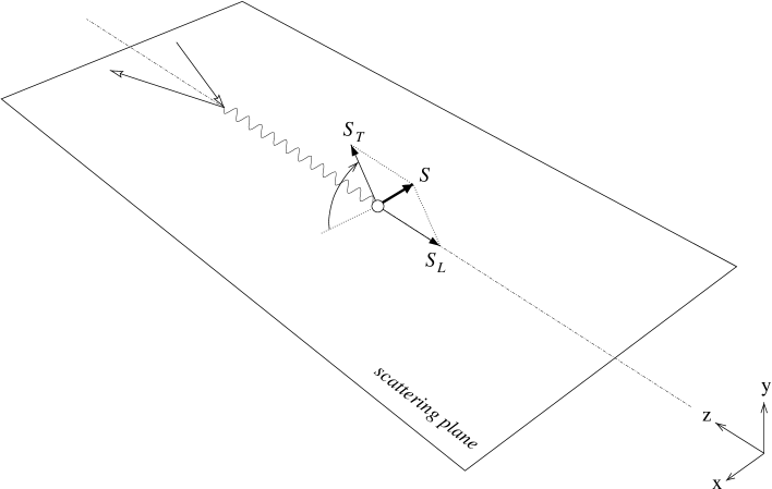
Figure 2.2: Description of the vectors involved in totally inclusive deep inelastic scattering and of the azimuthal angle $\phi_{S}$.

Considering the lepton to be longitudinally polarized, in the massless limit the leptonic tensor is given by [141]

$$\begin{split}L_{\mu\nu}&=\sum_{\lambda_{e}^{\prime}}\Bigl{(}\mspace{5.0mu}\makebox[0.0pt]{$\bar{\phantom{u}}$}\mspace{-5.0mu}{u}\mspace{-5.0mu}\makebox[0.0pt]{$\bar{\phantom{u}}$}\mspace{5.0mu}(l^{\prime},\lambda_{e}^{\prime})\,\gamma_{\mu}\,u(l,\lambda_{e})\Bigr{)}^{*}\;\Bigl{(}\mspace{5.0mu}\makebox[0.0pt]{$\bar{\phantom{u}}$}\mspace{-5.0mu}{u}\mspace{-5.0mu}\makebox[0.0pt]{$\bar{\phantom{u}}$}\mspace{5.0mu}(l^{\prime},\lambda_{e}^{\prime})\,\gamma_{\nu}\,u(l,\lambda_{e})\Bigr{)}\\ &=-Q^{2}g_{\mu\nu}+2\left(l_{\mu}l^{\prime}_{\nu}+l^{\prime}_{\mu}l_{\nu}\right)+2{\rm i}\,\lambda_{e}\,\epsilon_{\mu\nu\rho\sigma}\,l^{\rho}l^{\prime\sigma}.\end{split}$$ (2.7)

The leptonic tensor contains all the information on the leptonic probe, which can be described by means of perturbative QED, while the information on the hadronic target is contained in the hadronic tensor

$$2MW^{\mu\nu}(q,P,S) =\frac{1}{2\pi}\sum_{\cal X}\int\frac{\operatorname{{\rm\,d}}^{3}\!\bm{P}_{{\cal X}}}{(2\pi)^{3}\,2P_{{\cal X}}^{0}}\;(2\pi)^{4}\,\delta^{(4)}\Bigl{(}q+P-P_{{\cal X}}\Bigr{)}\,H^{\mu\nu}(P,S,P_{\cal X}),$$ (2.8)

$$H^{\mu\nu}(P,S,P_{\cal X}) =\bigl{\langle}{P,S}\mspace{2.0mu}\raisebox{-3.0pt}{\rule{0.7pt}{12.0pt}}\;J^{\mu}(0)\;\raisebox{-3.0pt}{\rule{0.7pt}{12.0pt}}\,{\cal X}\bigr{\rangle}\bigl{\langle}{\cal X}\mspace{2.0mu}\raisebox{-3.0pt}{\rule{0.7pt}{12.0pt}}\;J^{\nu}(0)\;\raisebox{-3.0pt}{\rule{0.7pt}{12.0pt}}\,{P,S}\bigr{\rangle}.$$ (2.9)

The state ${\cal X}$ symbolizes any final state, with total momentum $P_{\cal X}$. It is integrated over since in inclusive processes the final state goes undetected. By Fourier transforming the delta function and translating one of the current operators, we can rewrite the hadronic tensor as

$$2MW^{\mu\nu}(q,P,S)=\frac{1}{2\pi}\int\operatorname{{\rm\,d}}^{4}\!\xi\;{\rm e}^{{\rm i}q\cdot\xi}\;\bigl{\langle}{P,S}\mspace{2.0mu}\raisebox{-3.0pt}{\rule{0.7pt}{12.0pt}}\;J^{\mu}(\xi)\,J^{\nu}(0)\;\raisebox{-3.0pt}{\rule{0.7pt}{12.0pt}}\,{P,S}\bigr{\rangle}.$$ (2.10)

In general, the structure of the hadronic tensor cannot be specified further, because this would require an understanding of its inner dynamics. At most, it can be parametrized in terms of structure functions. However, the phenomenology of DIS taught us that at sufficiently high $Q^{2}$ we can assume that the scattering of the electron takes place off a quark of mass $m$ inside the nucleon. The final state ${\cal X}$ can be split in a quark with momentum $k$ plus a state $X$ with momentum $P_{X}$. Considering the electron-quark interaction at tree level only, the hadronic tensor can be written as

$$\begin{split}2MW^{\mu\nu}(q,P,S)&=\frac{1}{2\pi}\sum_{q}e_{q}^{2}\sum_{X}\int\frac{\operatorname{{\rm\,d}}^{3}\!\bm{P}_{X}}{(2\pi)^{3}\,2P_{X}^{0}}\int\frac{\operatorname{{\rm\,d}}^{3}\!\bm{k}}{(2\pi)^{3}\,2k^{0}}\;(2\pi)^{4}\,\delta^{(4)}\Bigl{(}P+q-k-P_{X}\Bigr{)}\\ &\quad\times\Bigl{(}\bigl{\langle}{P,S}\mspace{2.0mu}\raisebox{-3.0pt}{\rule{0.7pt}{12.0pt}}\;\mspace{5.0mu}\makebox[0.0pt]{$\bar{\phantom{\psi}}$}\mspace{-5.0mu}{\psi}\mspace{-5.0mu}\makebox[0.0pt]{$\bar{\phantom{\psi}}$}\mspace{5.0mu}_{i}(0)\;\raisebox{-3.0pt}{\rule{0.7pt}{12.0pt}}\,{X}\bigr{\rangle}\bigl{\langle}{X}\mspace{2.0mu}\raisebox{-3.0pt}{\rule{0.7pt}{12.0pt}}\;\psi_{j}(0)\;\raisebox{-3.0pt}{\rule{0.7pt}{12.0pt}}\,{P,S}\bigr{\rangle}\,\gamma^{\mspace{2.0mu}\mu}_{ik}\left(\makebox[0.0pt][l]{$\sslash$}{k}+m\right)_{kl}\gamma^{\nu}_{lj}\\ &\quad+\bigl{\langle}{P,S}\mspace{2.0mu}\raisebox{-3.0pt}{\rule{0.7pt}{12.0pt}}\;\psi_{j}(0)\;\raisebox{-3.0pt}{\rule{0.7pt}{12.0pt}}\,{X}\bigr{\rangle}\bigl{\langle}{X}\mspace{2.0mu}\raisebox{-3.0pt}{\rule{0.7pt}{12.0pt}}\;\mspace{5.0mu}\makebox[0.0pt]{$\bar{\phantom{\psi}}$}\mspace{-5.0mu}{\psi}\mspace{-5.0mu}\makebox[0.0pt]{$\bar{\phantom{\psi}}$}\mspace{5.0mu}_{i}(0)\;\raisebox{-3.0pt}{\rule{0.7pt}{12.0pt}}\,{P,S}\bigr{\rangle}\,\gamma^{\nu}_{ik}\left(\makebox[0.0pt][l]{$\sslash$}{k}-m\right)_{kl}\gamma^{\mspace{2.0mu}\mu}_{lj}\Bigr{)},\end{split}$$ (2.11)

where $k$ is the momentum of the struck quark, the index $q$ denotes the quark flavor and $e_{q}$ is the fractional charge of the quark. Note that, for simplicity, we omitted the flavor indices on the quark fields. The integration over the phase space of the final-state quark can be replaced by a four-dimensional integral with an on-shell condition, so that the hadronic tensor can be rewritten as

$$\begin{split}2MW^{\mu\nu}(q,P,S)&=\sum_{q}e_{q}^{2}\sum_{X}\int\frac{\operatorname{{\rm\,d}}^{3}\!\bm{P}_{X}}{(2\pi)^{3}\,2P_{X}^{0}}\int\operatorname{{\rm\,d}}^{4}\!k\;\delta\left(k^{2}-m^{2}\right)\,\theta\left(k^{0}-m\right)\\ &\quad\times\delta^{(4)}\Bigl{(}P+q-k-P_{X}\Bigr{)}\,\Bigl{(}\bigl{\langle}{P,S}\mspace{2.0mu}\raisebox{-3.0pt}{\rule{0.7pt}{12.0pt}}\;\mspace{5.0mu}\makebox[0.0pt]{$\bar{\phantom{\psi}}$}\mspace{-5.0mu}{\psi}\mspace{-5.0mu}\makebox[0.0pt]{$\bar{\phantom{\psi}}$}\mspace{5.0mu}_{i}(0)\;\raisebox{-3.0pt}{\rule{0.7pt}{12.0pt}}\,{X}\bigr{\rangle}\bigl{\langle}{X}\mspace{2.0mu}\raisebox{-3.0pt}{\rule{0.7pt}{12.0pt}}\;\psi_{j}(0)\;\raisebox{-3.0pt}{\rule{0.7pt}{12.0pt}}\,{P,S}\bigr{\rangle}\,\gamma^{\mspace{2.0mu}\mu}_{ik}\left(\makebox[0.0pt][l]{$\sslash$}{k}+m\right)_{kl}\gamma^{\nu}_{lj}\\ &\quad+\bigl{\langle}{P,S}\mspace{2.0mu}\raisebox{-3.0pt}{\rule{0.7pt}{12.0pt}}\;\psi_{j}(0)\;\raisebox{-3.0pt}{\rule{0.7pt}{12.0pt}}\,{X}\bigr{\rangle}\bigl{\langle}{X}\mspace{2.0mu}\raisebox{-3.0pt}{\rule{0.7pt}{12.0pt}}\;\mspace{5.0mu}\makebox[0.0pt]{$\bar{\phantom{\psi}}$}\mspace{-5.0mu}{\psi}\mspace{-5.0mu}\makebox[0.0pt]{$\bar{\phantom{\psi}}$}\mspace{5.0mu}_{i}(0)\;\raisebox{-3.0pt}{\rule{0.7pt}{12.0pt}}\,{P,S}\bigr{\rangle}\,\gamma^{\nu}_{ik}\left(\makebox[0.0pt][l]{$\sslash$}{k}-m\right)_{kl}\gamma^{\mspace{2.0mu}\mu}_{lj}\Bigr{)}.\end{split}$$ (2.12)

Next, we Fourier transform the Dirac delta function and we introduce the momentum $p=k-q$ to obtain

$$\begin{split}2MW^{\mu\nu}(q,P,S)&=\sum_{q}e_{q}^{2}\sum_{X}\int\frac{\operatorname{{\rm\,d}}^{3}\!\bm{P}_{X}}{(2\pi)^{3}\,2P_{X}^{0}}\int\operatorname{{\rm\,d}}^{4}\!p\;\delta\left(\bigl{(}p+q\bigr{)}^{2}-m^{2}\right)\,\\ &\quad\times\theta\left(p^{0}+q^{0}-m\right)\int\frac{\operatorname{{\rm\,d}}^{4}\!\xi}{(2\pi)^{4}}\,{\rm e}^{{\rm i}\,(P-p-P_{X})\cdot\xi}\;\\ &\quad\times\Bigl{(}\bigl{\langle}{P,S}\mspace{2.0mu}\raisebox{-3.0pt}{\rule{0.7pt}{12.0pt}}\;\mspace{5.0mu}\makebox[0.0pt]{$\bar{\phantom{\psi}}$}\mspace{-5.0mu}{\psi}\mspace{-5.0mu}\makebox[0.0pt]{$\bar{\phantom{\psi}}$}\mspace{5.0mu}_{i}(0)\;\raisebox{-3.0pt}{\rule{0.7pt}{12.0pt}}\,{X}\bigr{\rangle}\bigl{\langle}{X}\mspace{2.0mu}\raisebox{-3.0pt}{\rule{0.7pt}{12.0pt}}\;\psi_{j}(0)\;\raisebox{-3.0pt}{\rule{0.7pt}{12.0pt}}\,{P,S}\bigr{\rangle}\,\gamma^{\mspace{2.0mu}\mu}_{ik}\left(\makebox[0.0pt][l]{\hskip 1.3pt$\sslash$}{p}+\makebox[0.0pt][l]{\hskip 0.3pt$\sslash$}{q}+m\right)_{kl}\gamma^{\nu}_{lj}\\ &\quad+\bigl{\langle}{P,S}\mspace{2.0mu}\raisebox{-3.0pt}{\rule{0.7pt}{12.0pt}}\;\psi_{j}(0)\;\raisebox{-3.0pt}{\rule{0.7pt}{12.0pt}}\,{X}\bigr{\rangle}\bigl{\langle}{X}\mspace{2.0mu}\raisebox{-3.0pt}{\rule{0.7pt}{12.0pt}}\;\mspace{5.0mu}\makebox[0.0pt]{$\bar{\phantom{\psi}}$}\mspace{-5.0mu}{\psi}\mspace{-5.0mu}\makebox[0.0pt]{$\bar{\phantom{\psi}}$}\mspace{5.0mu}_{i}(0)\;\raisebox{-3.0pt}{\rule{0.7pt}{12.0pt}}\,{P,S}\bigr{\rangle}\,\gamma^{\nu}_{ik}\left(\makebox[0.0pt][l]{\hskip 1.3pt$\sslash$}{p}+\makebox[0.0pt][l]{\hskip 0.3pt$\sslash$}{q}-m\right)_{kl}\gamma^{\mspace{2.0mu}\mu}_{lj}\Bigr{)}.\end{split}$$ (2.13)

Finally, we use part of the exponential to perform a translation of the field operators and we use completeness to eliminate the unobserved $X$ states, so that

$$\begin{split}2MW^{\mu\nu}(q,P,S)&=\sum_{q}e_{q}^{2}\int\operatorname{{\rm\,d}}^{4}\!p\;\delta\left(\bigl{(}p+q\bigr{)}^{2}-m^{2}\right)\,\theta\left(p^{0}+q^{0}-m\right)\int\frac{\operatorname{{\rm\,d}}^{4}\!\xi}{(2\pi)^{4}}\,{\rm e}^{-{\rm i}p\cdot\xi}\\ &\quad\times\Bigl{(}\bigl{\langle}{P,S}\mspace{2.0mu}\raisebox{-3.0pt}{\rule{0.7pt}{12.0pt}}\;\mspace{5.0mu}\makebox[0.0pt]{$\bar{\phantom{\psi}}$}\mspace{-5.0mu}{\psi}\mspace{-5.0mu}\makebox[0.0pt]{$\bar{\phantom{\psi}}$}\mspace{5.0mu}_{i}(\xi)\;\psi_{j}(0)\;\raisebox{-3.0pt}{\rule{0.7pt}{12.0pt}}\,{P,S}\bigr{\rangle}\,\gamma^{\mspace{2.0mu}\mu}_{ik}\left(\makebox[0.0pt][l]{\hskip 1.3pt$\sslash$}{p}+\makebox[0.0pt][l]{\hskip 0.3pt$\sslash$}{q}+m\right)_{kl}\gamma^{\nu}_{lj}\\ &\quad+\bigl{\langle}{P,S}\mspace{2.0mu}\raisebox{-3.0pt}{\rule{0.7pt}{12.0pt}}\;\psi_{j}(\xi)\;\mspace{5.0mu}\makebox[0.0pt]{$\bar{\phantom{\psi}}$}\mspace{-5.0mu}{\psi}\mspace{-5.0mu}\makebox[0.0pt]{$\bar{\phantom{\psi}}$}\mspace{5.0mu}_{i}(0)\;\raisebox{-3.0pt}{\rule{0.7pt}{12.0pt}}\,{P,S}\bigr{\rangle}\,\gamma^{\nu}_{ik}\left(\makebox[0.0pt][l]{\hskip 1.3pt$\sslash$}{p}+\makebox[0.0pt][l]{\hskip 0.3pt$\sslash$}{q}-m\right)_{kl}\gamma^{\mspace{2.0mu}\mu}_{lj}\Bigr{)}.\end{split}$$ (2.14)

The hadronic tensor can be written in a more compact way by introducing the quark-quark correlation function $\Phi$ and the antiquark-antiquark correlation function $\mspace{5.0mu}\makebox[0.0pt]{$\bar{\phantom{\Phi}}$}\mspace{-5.0mu}{\Phi}\mspace{-5.0mu}\makebox[0.0pt]{$\bar{\phantom{\Phi}}$}\mspace{5.0mu}$

$$\begin{split}2MW^{\mu\nu}(q,P,S)&=\sum_{q}e_{q}^{2}\int\operatorname{{\rm\,d}}^{4}\!p\;\delta\left(\bigl{(}p+q\bigr{)}^{2}-m^{2}\right)\,\theta\left(p^{0}+q^{0}-m\right)\\ &\quad\times\operatorname{Tr}\left[\Phi(p,P,S)\gamma^{\mspace{2.0mu}\mu}\left(\makebox[0.0pt][l]{\hskip 1.3pt$\sslash$}{p}+\makebox[0.0pt][l]{\hskip 0.3pt$\sslash$}{q}+m\right)\gamma^{\nu}+\mspace{5.0mu}\makebox[0.0pt]{$\bar{\phantom{\Phi}}$}\mspace{-5.0mu}{\Phi}\mspace{-5.0mu}\makebox[0.0pt]{$\bar{\phantom{\Phi}}$}\mspace{5.0mu}(p,P,S)\gamma^{\nu}\left(\makebox[0.0pt][l]{\hskip 1.3pt$\sslash$}{p}+\makebox[0.0pt][l]{\hskip 0.3pt$\sslash$}{q}-m\right)\gamma^{\mspace{2.0mu}\mu}\right]\end{split}$$ (2.15)

where

$$\begin{split}\Phi_{ji}(p,P,S)&=\frac{1}{(2\pi)^{4}}\int\operatorname{{\rm\,d}}^{4}\!\xi\;{\rm e}^{-{\rm i}p\cdot\xi}\bigl{\langle}{P,S}\mspace{2.0mu}\raisebox{-3.0pt}{\rule{0.7pt}{12.0pt}}\;\mspace{5.0mu}\makebox[0.0pt]{$\bar{\phantom{\psi}}$}\mspace{-5.0mu}{\psi}\mspace{-5.0mu}\makebox[0.0pt]{$\bar{\phantom{\psi}}$}\mspace{5.0mu}_{i}(\xi)\;\psi_{j}(0)\;\raisebox{-3.0pt}{\rule{0.7pt}{12.0pt}}\,{P,S}\bigr{\rangle}\\ &=\sum_{X}\int\frac{\operatorname{{\rm\,d}}^{3}\!\bm{P}_{X}}{(2\pi)^{3}\,2P_{X}^{0}}\;\bigl{\langle}{P,S}\mspace{2.0mu}\raisebox{-3.0pt}{\rule{0.7pt}{12.0pt}}\;\mspace{5.0mu}\makebox[0.0pt]{$\bar{\phantom{\psi}}$}\mspace{-5.0mu}{\psi}\mspace{-5.0mu}\makebox[0.0pt]{$\bar{\phantom{\psi}}$}\mspace{5.0mu}_{i}(0)\;\raisebox{-3.0pt}{\rule{0.7pt}{12.0pt}}\,{X}\bigr{\rangle}\bigl{\langle}{X}\mspace{2.0mu}\raisebox{-3.0pt}{\rule{0.7pt}{12.0pt}}\;\psi_{j}(0)\;\raisebox{-3.0pt}{\rule{0.7pt}{12.0pt}}\,{P,S}\bigr{\rangle}\;\delta^{(4)}\Bigl{(}P-p-P_{X}\Bigr{)},\end{split}$$ (2.16a)

$$\begin{split}\mspace{5.0mu}\makebox[0.0pt]{$\bar{\phantom{\Phi}}$}\mspace{-5.0mu}{\Phi}\mspace{-5.0mu}\makebox[0.0pt]{$\bar{\phantom{\Phi}}$}\mspace{5.0mu}_{ji}(p,P,S)&=\frac{1}{(2\pi)^{4}}\int\operatorname{{\rm\,d}}^{4}\!\xi\;{\rm e}^{-{\rm i}p\cdot\xi}\bigl{\langle}{P,S}\mspace{2.0mu}\raisebox{-3.0pt}{\rule{0.7pt}{12.0pt}}\;\psi_{j}(\xi)\;\mspace{5.0mu}\makebox[0.0pt]{$\bar{\phantom{\psi}}$}\mspace{-5.0mu}{\psi}\mspace{-5.0mu}\makebox[0.0pt]{$\bar{\phantom{\psi}}$}\mspace{5.0mu}_{i}(0)\;\raisebox{-3.0pt}{\rule{0.7pt}{12.0pt}}\,{P,S}\bigr{\rangle}\\ &=\sum_{X}\int\frac{\operatorname{{\rm\,d}}^{3}\!\bm{P}_{X}}{(2\pi)^{3}\,2P_{X}^{0}}\;\bigl{\langle}{P,S}\mspace{2.0mu}\raisebox{-3.0pt}{\rule{0.7pt}{12.0pt}}\;\psi_{j}(0)\;\raisebox{-3.0pt}{\rule{0.7pt}{12.0pt}}\,{X}\bigr{\rangle}\bigl{\langle}{X}\mspace{2.0mu}\raisebox{-3.0pt}{\rule{0.7pt}{12.0pt}}\;\mspace{5.0mu}\makebox[0.0pt]{$\bar{\phantom{\psi}}$}\mspace{-5.0mu}{\psi}\mspace{-5.0mu}\makebox[0.0pt]{$\bar{\phantom{\psi}}$}\mspace{5.0mu}_{i}(0)\;\raisebox{-3.0pt}{\rule{0.7pt}{12.0pt}}\,{P,S}\bigr{\rangle}\;\delta^{(4)}\Bigl{(}P-p-P_{X}\Bigr{)}.\end{split}$$ (2.16b)

As the quark fields should carry a flavor index that we omitted, also the correlation functions are flavor dependent and they should be indicated more appropriately as $\Phi^{q}$ and $\mspace{5.0mu}\makebox[0.0pt]{$\bar{\phantom{\Phi}}$}\mspace{-5.0mu}{\Phi}\mspace{-5.0mu}\makebox[0.0pt]{$\bar{\phantom{\Phi}}$}\mspace{5.0mu}^{q}$. For simplicity, $\mspace{5.0mu}\makebox[0.0pt]{$\bar{\phantom{\Phi}}$}\mspace{-5.0mu}{\Phi}\mspace{-5.0mu}\makebox[0.0pt]{$\bar{\phantom{\Phi}}$}\mspace{5.0mu}$ will be omitted henceforth. It can be accounted for simply by extending the summation over quarks to a summation over quarks and antiquarks. A graphical representation of the hadronic tensor at tree level in the parton model is given by the so-called handbag diagram, depicted in Fig. 2.3.

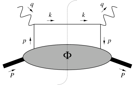
Figure 2.3: The handbag diagram, describing the hadronic tensor at tree level.

We parametrize the quark momentum $p$ in the following way

$$p^{\mspace{2.0mu}\mu}=\left[\frac{p^{2}+|\bm{p}_{T}|^{2}}{2xP^{+}},\;xP^{+},\;\bm{p}_{T}\right].$$ (2.17)

In our approach, we assume that neither the virtuality of the quark, $p^{2}$, nor its transverse momentum squared, $|\bm{p}_{T}|^{2}$, can be large in comparison with the hard scale $Q^{2}$. Under these conditions, the quark momentum is soft with respect to the hadron momentum and its relevant component is $xP^{+}$. In Eq. (2.15), neglecting terms which are $1/Q$ suppressed, we can use an approximate expression for the delta function and

$$2MW^{\mu\nu}(q,P,S) \approx\sum_{q}e_{q}^{2}\int\operatorname{{\rm\,d}}^{2}\!\bm{p}_{T}\operatorname{{\rm\,d}}p^{-}\operatorname{{\rm\,d}}x\;\frac{P^{+}}{2P\cdot q}\;\delta\left(x-x_{B}\right)\,\operatorname{Tr}\left[\Phi(p,P,S)\,\gamma^{\mspace{2.0mu}\mu}\left(\makebox[0.0pt][l]{\hskip 1.3pt$\sslash$}{p}+\makebox[0.0pt][l]{\hskip 0.3pt$\sslash$}{q}+m\right)\gamma^{\nu}\right]$$

$$=\sum_{q}e_{q}^{2}\;\frac{1}{2}\operatorname{Tr}\left[\Phi(x_{B},S)\,\gamma^{\mspace{2.0mu}\mu}\frac{P^{+}}{P\cdot q}\left(\makebox[0.0pt][l]{\hskip 1.3pt$\sslash$}{p}+\makebox[0.0pt][l]{\hskip 0.3pt$\sslash$}{q}+m\right)\gamma^{\nu}\right]$$ (2.18)

where we introduced the integrated correlation function

$$\begin{split}\Phi_{ji}(x,S)&=\int\operatorname{{\rm\,d}}^{2}\!\bm{p}_{T}\operatorname{{\rm\,d}}p^{-}\;\Phi_{ji}(p,P,S)\biggr{|}_{p^{+}=xP^{+}}\\ &=\int\frac{\operatorname{{\rm\,d}}\xi^{-}}{2\pi}\;{\rm e}^{-{\rm i}p\cdot\xi}\bigl{\langle}{P,S}\mspace{2.0mu}\raisebox{-3.0pt}{\rule{0.7pt}{12.0pt}}\;\mspace{5.0mu}\makebox[0.0pt]{$\bar{\phantom{\psi}}$}\mspace{-5.0mu}{\psi}\mspace{-5.0mu}\makebox[0.0pt]{$\bar{\phantom{\psi}}$}\mspace{5.0mu}_{i}(\xi)\;\psi_{j}(0)\;\raisebox{-3.0pt}{\rule{0.7pt}{12.0pt}}\,{P,S}\bigr{\rangle}\biggr{|}_{\xi^{+}=\bm{\xi}_{T}=0}.\end{split}$$ (2.19)

Notice that there is a contradiction between the fact that we assumed the transverse momentum of the quark to be small in comparison to the hard scale, yet we are integrating over the entire space of $\bm{p}_{T}$. Indeed, when dealing with transverse momentum of perturbative origin (i.e. arising from the radiation of gluons, see next section), which typically falls down as $1/|\bm{p}_{T}|^{2}$, we have to impose a cut-off on the maximum value the transverse momentum can reach. This cut-off depends on the scale $Q^{2}$. On the other hand, the transverse momentum of nonperturbative origin, usually called intrinsic transverse momentum, is supposed to fall off very rapidly so that there is effectively almost no intrinsic transverse momentum above a typical scale of 1 GeV².

Finally, from the outgoing quark momentum, $p+q$, we can select only the minus component and obtain the final form for the hadronic tensor at leading twist

$$2MW^{\mu\nu}(q,P,S)\approx\sum_{q}e_{q}^{2}\;\frac{1}{2}\operatorname{Tr}\left[\Phi(x_{B},S)\,\gamma^{\mspace{2.0mu}\mu}\gamma^{+}\gamma^{\nu}\right].$$ (2.20)

A few words to justify the last approximation are in order. The dominance of the minus component is most easily seen in the infinite momentum frame, where $p^{-}\!+q^{-}$ is of the order of $Q$, while $p^{+}\!+q^{+}=0$, and $\bm{p}_{T}$ and $m$ are of the order of 1. However, if we perform a $1/Q$ expansion of the full expression, including the correlation function $\Phi$ [starting from Eq. (2.31)], we would be able to check that in any collinear frame the dominant terms arise only from the combination of plus component in the correlation function and minus components in the outgoing quark momentum.

2.1.3 One gluon additions

Up to now, we took into consideration only quark-quark correlation functions at tree level. The addition of a gluon can either lead to the introduction of a quark-gluon-quark correlation function or can give rise to perturbative corrections to the photon-quark scattering [82]. In this thesis, we will not take quark-gluon-quark correlation functions into account, since they start contributing only at the twist-three level, and we will not examine perturbative corrections, since they give only origin to a logarithmic scale dependence of the quark-quark functions. Nevertheless, for completeness we will now give a sketchy view of these very important issues.

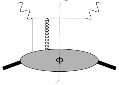
Figure 2.4: One gluon addition: gluon coming from the soft blob.

When the gluons come directly from the soft blob, as in the diagram of Fig. 2.4, longitudinally polarized gluons ($A^{+}$) are the dominant ones, while transversely polarized gluons ($A_{T}$) are subject to a $1/Q$ suppression. If we choose a physical gauge where $A^{+}=0$, then this kind of diagrams contribute only at twist three and higher and they require the introduction of quark-gluon-quark correlators [94]. On the other hand, in a different gauge the contributions of longitudinal gluons is present and is not necessarily suppressed by any power of $1/Q$. Then, we have to sum all the contributions with an arbitrary number of longitudinal gluons. The result of this summation can be cast in the form of a gauge link to be inserted in the definition of the quark-quark correlation function

$$\Phi_{ji}(p,P,S)=\frac{1}{(2\pi)^{4}}\int\operatorname{{\rm\,d}}^{4}\!\xi\;{\rm e}^{-{\rm i}p\cdot\xi}\bigl{\langle}{P,S}\mspace{2.0mu}\raisebox{-3.0pt}{\rule{0.7pt}{12.0pt}}\;\mspace{5.0mu}\makebox[0.0pt]{$\bar{\phantom{\psi}}$}\mspace{-5.0mu}{\psi}\mspace{-5.0mu}\makebox[0.0pt]{$\bar{\phantom{\psi}}$}\mspace{5.0mu}_{i}(\xi)\,{\cal L}(\xi,0;\mbox{path})\,\psi_{j}(0)\;\raisebox{-3.0pt}{\rule{0.7pt}{12.0pt}}\,{P,S}\bigr{\rangle}$$ (2.21)

where the gauge link is a path-ordered exponential

$${\cal L}(\xi,0;\mbox{path})={\cal P}\exp\left(-{\rm i}g_{s}\int_{0}^{\xi}\operatorname{{\rm\,d}}s^{\mu}A_{\mu}(s)\right).$$ (2.22)

with a straight path along the light-cone minus direction [58, 94].

In $A^{+}=0$ gauges the link is equal to unity (although some subleties have been recently analyzed in Ref. 71). We will henceforth neglect it and trade off manifest color gauge invariance for a lighter notation. Finally, we mention that recently it has been suggested that the gauge link could play an important role in the context of T-odd distribution functions [78] (see Sec. 2.4). In particular, much care should be taken when including partonic transverse momentum. In this case, the gauge link path cannot simply run along the light-cone but has to have a transverse component and it might not be reducible to unity anymore [124, 78].

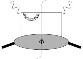
Figure 2.5: One gluon addition: virtual loop diagrams.

Now we take a brief look to perturbative corrections to the quark-quark correlation function (see Refs. 96 and 147). They are of two kinds: virtual gluon loop diagrams (Fig. 2.5) and real gluon bremsstrahlung diagrams (Fig. 2.6). Each virtual diagram contains ultraviolet and infrared divergences. The ultraviolet divergences can be cured using standard renormalization techniques. The infrared divergences cancel with analogous divergences in the real gluon emission diagrams [96].

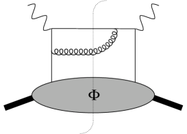
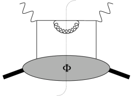
Figure 2.6: One gluon addition: real loop diagrams.

The remaining parts of the diagrams give actual $\alpha_{s}$ corrections to the tree level result of the previous section. In particular, collinear divergences give origin to the leading-log part of the evolution equations, by which the parton distribution functions (see Sec. 2.2) acquire a dependence on the scale $Q^{2}$ [100, 12, 88].

2.1.4 Leading twist part and connection with helicity formalism

To identify the leading twist contributions to the cross section, it is convenient to define the projectors

$${\cal P}_{+} =\frac{1}{2}\;\gamma^{-}\gamma^{+}, {\cal P}_{-} =\frac{1}{2}\;\gamma^{+}\gamma^{-}.$$ (2.23)

Before the interaction with the virtual photon, the relevant components of the quark fields are the plus components, $\psi_{+}={\cal P}_{+}\,\psi$. They are usually referred to as the good components. Vice versa, after the interaction with the virtual photon, the relevant components of the outgoing quark fields are the minus components, $\psi_{-}={\cal P}_{-}\,\psi$. Therefore, the leading twist part of the hadronic tensor in Eq. (2.18) can be projected out in the following way (see Fig. 2.7)

$$\begin{split}2MW^{\mu\nu}(q,P,S)&\approx\sum_{q}e_{q}^{2}\,\operatorname{Tr}{\left[{\cal P}_{+}\,\Phi(x_{B},S)\;{\cal P}_{-}\;\gamma^{\mu}\;{\cal P}_{-}\,\frac{P^{+}}{2P\cdot q}\left(\makebox[0.0pt][l]{\hskip 1.3pt$\sslash$}{p}+\makebox[0.0pt][l]{\hskip 0.3pt$\sslash$}{q}+m\right)\;{\cal P}_{+}\;\gamma^{\nu}\right]}\\ &=\sum_{q}e_{q}^{2}\,\operatorname{Tr}{\left[{\cal P}_{+}\,\Phi(x_{B},S)\,\gamma^{+}\;\frac{\gamma^{-}\gamma^{\mu}}{2}\,{\cal P}_{-}\;{\cal P}_{-}\,\frac{P^{+}}{2P\cdot q}\left(\makebox[0.0pt][l]{\hskip 1.3pt$\sslash$}{p}+\makebox[0.0pt][l]{\hskip 0.3pt$\sslash$}{q}+m\right)\,\gamma^{-}\;\frac{\gamma^{+}\gamma^{\nu}}{2}\,{\cal P}_{+}\right]}.\end{split}$$ (2.24)

Figure 2.7: Graphical representation of the insertion of the good projectors to isolate the leading part of the hadronic tensor.

The differential cross section defined in Eq. (2.6) takes the form

$$\begin{split}\@ADDCLASS{ltx_eqn_lefteqn}$\displaystyle\frac{\operatorname{{\rm\,d}}^{3}\!\sigma}{\operatorname{{\rm\,d}}x_{B}\operatorname{{\rm\,d}}y\operatorname{{\rm\,d}}\phi_{S}}$\mbox{}\hfil\\ &\approx\sum_{q}\,\frac{\alpha^{2}e_{q}^{2}}{2\,s\,x_{B}\,Q^{2}}\,L_{\mu\nu}(l,l^{\prime},\lambda_{e})\;\operatorname{Tr}{\left[{\cal P}_{+}\,\Phi(x_{B},S)\,\gamma^{+}\;\frac{\gamma^{-}\gamma^{\mu}}{2}\,{\cal P}_{-}\;{\cal P}_{-}\,\frac{P^{+}}{2P\cdot q}\left(\makebox[0.0pt][l]{\hskip 1.3pt$\sslash$}{p}+\makebox[0.0pt][l]{\hskip 0.3pt$\sslash$}{q}+m\right)\,\gamma^{-}\;\frac{\gamma^{+}\gamma^{\nu}}{2}\,{\cal P}_{+}\right]}\\ &\approx\sum_{q}\,\Bigl{(}{\cal P}_{+}\,\Phi(x_{B},S)\gamma^{+}\Bigr{)}_{ji}\left[\frac{\alpha^{2}e_{q}^{2}}{s\,x_{B}\,Q^{2}}\,L_{\mu\nu}(l,l^{\prime},\lambda_{e})\left(\frac{\gamma^{-}\gamma^{\mu}}{2}\,{\cal P}_{-}\right)_{il}\left(\frac{\gamma^{+}\gamma^{\nu}}{2}\,{\cal P}_{+}\right)_{mj}\right]\left(\frac{{\cal P}_{-}}{2}\right)_{lm},\end{split}$$ (2.25)

where we explicitly showed Dirac indices (repeated indices are summed over). In Sec. 2.2.1, we will see in detail how the insertion of the projectors effectively reduces the four-dimensional Dirac space into a two-dimensional subspace. Chiral-right and chiral-left good quark spinors can be used as a basis in this space. Therefore, it is possible to replace the Dirac indices with chirality indices (of good fields). By doing this, we put particular evidence on the connection with the helicity/chirality formalism (see e.g. Refs. 112 and 19). In fact, the cross section can be conveniently rewritten as

$$\frac{\operatorname{{\rm\,d}}^{3}\!\sigma}{\operatorname{{\rm\,d}}x_{B}\operatorname{{\rm\,d}}y\operatorname{{\rm\,d}}\phi_{S}}\approx\frac{1}{2}\sum_{q}\;\Bigl{(}{\cal P}_{+}\,\Phi(x_{B},S)\gamma^{+}\Bigr{)}_{\chi^{\prime}_{1}\chi^{\phantom{{}^{\prime}}}_{1}}\;\Bigl{(}\frac{\operatorname{{\rm\,d}}\sigma^{eq}}{\operatorname{{\rm\,d}}y}\Bigr{)}^{\chi^{\phantom{{}^{\prime}}}_{1}\chi^{\prime}_{1}},$$ (2.26)

where the elementary electron-quark cross section is

$$\begin{split}\Bigl{(}\frac{\operatorname{{\rm\,d}}\sigma^{eq}}{\operatorname{{\rm\,d}}y}\Bigr{)}^{\chi^{\phantom{{}^{\prime}}}_{1}\chi^{\prime}_{1}}&=\frac{\alpha^{2}e_{q}^{2}}{sx_{B}Q^{2}}\,L_{\mu\nu}(l,l^{\prime},\lambda_{e})\left(\frac{\gamma^{-}\gamma^{\mu}}{2}\,{\cal P}_{-}\right)^{\chi^{\phantom{{}^{\prime}}}_{1}\chi^{\phantom{{}^{\prime}}}_{2}}\left(\frac{\gamma^{+}\gamma^{\nu}}{2}\,{\cal P}_{+}\right)^{\chi^{\prime}_{2}\chi^{\prime}_{1}}\;\delta_{\chi^{\phantom{{}^{\prime}}}_{2}\chi^{\prime}_{2}}\\[8.53581pt] &=\frac{\alpha^{2}e_{q}^{2}}{sx_{B}y^{2}}\,\begin{pmatrix}A(y)+\lambda_{e}C(y)&0\\ 0&A(y)-\lambda_{e}C(y)\end{pmatrix}.\end{split}$$ (2.27)

where

$$A(y) =1-y+\frac{y^{2}}{2}, C(y) =y\left(1-\frac{y}{2}\right).$$ (2.28)

Finally, we define the matrix $F=\Bigl{(}{\cal P}_{+}\,\Phi\gamma^{+}\Bigr{)}^{T}$, i.e. the transpose of the leading-twist part of the correlation function, and we observe that

$$\begin{split}F(x,S)_{\chi^{\phantom{{}^{\prime}}}_{1}\chi^{\prime}_{1}}&=\int\frac{\operatorname{{\rm\,d}}\xi^{-}}{2\pi\sqrt{2}}\;{\rm e}^{-{\rm i}p\cdot\xi}\bigl{\langle}{P,S}\mspace{2.0mu}\raisebox{-3.0pt}{\rule{0.7pt}{12.0pt}}\;(\psi_{+})^{\dagger}_{\chi_{1}}(\xi)\;(\psi_{+})_{\chi^{\prime}_{1}}(0)\;\raisebox{-3.0pt}{\rule{0.7pt}{12.0pt}}\,{P,S}\bigr{\rangle}\biggr{|}_{\xi^{+}=\bm{\xi}_{T}=0}\\ &=\frac{1}{\sqrt{2}}\sum_{X}\int\frac{\operatorname{{\rm\,d}}^{3}\!\bm{P}_{X}}{(2\pi)^{3}\,2P_{X}^{0}}\,\bigl{\langle}{X}\mspace{2.0mu}\raisebox{-3.0pt}{\rule{0.7pt}{12.0pt}}\;(\psi_{+})_{\chi_{1}}(0)\;\raisebox{-3.0pt}{\rule{0.7pt}{12.0pt}}\,{P,S}\bigr{\rangle}^{\ast}\bigl{\langle}{X}\mspace{2.0mu}\raisebox{-3.0pt}{\rule{0.7pt}{12.0pt}}\;(\psi_{+})_{\chi^{\prime}_{1}}(0)\;\raisebox{-3.0pt}{\rule{0.7pt}{12.0pt}}\,{P,S}\bigr{\rangle}\;\delta\Bigl{(}\bigl{(}1-x\bigr{)}P^{+}-P^{+}_{X}\Bigr{)}.\end{split}$$ (2.29)

Thus, the transpose of the correlation function describes the forward scattering of a good antiquark off a hadron, or equivalently the forward scattering of an antiquark off a hadron in the infinite momentum frame. As any scattering matrix, for any antiquark-hadron state $\;\raisebox{-3.0pt}{\rule{0.7pt}{12.0pt}}\,{a}\bigr{\rangle}$ the expectation value $\bigl{\langle}{a\mspace{2.0mu}}\mspace{2.0mu}\raisebox{-3.0pt}{\rule{0.7pt}{12.0pt}}\;M\;\raisebox{-3.0pt}{\rule{0.7pt}{12.0pt}}\,{a}\bigr{\rangle}$ must be positive. In mathematical terms, this means that the matrix is positive semidefinite, i.e. the determinant of all the principal minors of the matrix has to be positive or zero. This property will prove to be essential in deriving bounds on the components of the correlation function, i.e. the parton distribution functions.

2.2 The correlation function $\Phi$

As shown in Eq. (2.16a), the quark-quark distribution correlation function, $\Phi$, can be expressed in terms of bilocal operators. At leading order in $1/Q$, it contains all the relevant information about the nonperturbative dynamics of the quarks inside the hadron. Due to its nonperturbative nature, it is not possible to calculate it from first principles, as we don’t know how the hadronic states are built up from the elementary quark and gluon fields.

When considering subleading orders in a $1/Q$ expansion, quark-gluon-quark correlation functions have to be considered, as we briefly mentioned in Sec. 2.1.3. In this case, the general structure of the hadronic tensor becomes richer. In the rest of the thesis, as the analysis will be concerned only with leading order terms, we will not deal with quark-gluon-quark correlation functions.

To get more insight into the information contained in the correlation function, which is a Dirac matrix, we can decompose it in a general way on a basis of Dirac structures. Each term of the decomposition can be a combination of the Lorentz vectors $p$ and $P$, the Lorentz pseudovector $S$ (in case of spin-half hadrons) and the Dirac structures

$${\bm{1}},\;\gamma_{5},\;\gamma^{\mu},\;\gamma^{\mu}\gamma_{5},\;{\rm i}\sigma^{\mu\nu}\gamma_{5}.$$

The spin vector can only appear linearly in the decomposition (cf. Eq. (2.43)). Moreover, each term of the full expression has to satisfy the conditions of Hermiticity and parity invariance

Hermiticity: $$\Phi(p,P,S) =\gamma^{0}\,\Phi^{{\dagger}}(p,P,S)\,\gamma^{0},$$ (2.30a)

parity: $$\Phi(p,P,S) =\gamma^{0}\,\Phi(\tilde{p},\tilde{P},-\tilde{S})\,\gamma^{0}$$ (2.30b)

where $\tilde{p}^{\nu}=\delta^{\nu\mu}p_{\mu}$ and so forth for the other vectors. The most general decomposition of the correlation function $\Phi$ imposing Hermiticity and parity invariance is [151, 141]

$$\begin{split}\Phi(p,P,S)&=M\,A_{1}\,{\bm{1}}+A_{2}\,\makebox[0.0pt][l]{\hskip 1.2pt$\sslash$}{P}+A_{3}\,\makebox[0.0pt][l]{\hskip 1.3pt$\sslash$}{p}+\frac{A_{4}}{M}\,\sigma_{\mu\nu}P^{\mspace{2.0mu}\mu}p^{\nu}+{\rm i}A_{5}\;p\cdot S\,\gamma_{5}\\ &\quad+M\,A_{6}\,\makebox[0.0pt][l]{\hskip 0.5pt$\sslash$}{S}\,\gamma_{5}+A_{7}\,\frac{p\cdot S}{M}\,\makebox[0.0pt][l]{\hskip 1.2pt$\sslash$}{P}\,\gamma_{5}+A_{8}\,\frac{p\cdot S}{M}\,\makebox[0.0pt][l]{\hskip 1.3pt$\sslash$}{p}\,\gamma_{5}+{\rm i}A_{9}\,\sigma_{\mu\nu}\gamma_{5}S^{\mu}P^{\nu}\\ &\quad+{\rm i}A_{10}\,\sigma_{\mu\nu}\gamma_{5}S^{\mu}p^{\nu}+{\rm i}A_{11}\,\frac{p\cdot S}{M^{2}}\,\sigma_{\mu\nu}\gamma_{5}P^{\mspace{2.0mu}\mu}p^{\nu}+A_{12}\,\frac{\epsilon_{\mu\nu\rho\sigma}\gamma^{\mspace{2.0mu}\mu}P^{\nu}p^{\rho}S^{\sigma}}{M},\end{split}$$ (2.31)

where the amplitudes $A_{i}$ are dimensionless real scalar functions $A_{i}=A_{i}(p\cdot P,p^{2})$.

The correlation function can be separated in a T-even part and a T-odd part, according to the definition

$$\Phi^{\ast}_{\text{T-even}}(p,P,S) ={\rm i}\gamma^{1}\gamma^{3}\,\Phi_{\text{T-even}}(\tilde{p},\tilde{P},\tilde{S})\,{\rm i}\gamma^{1}\gamma^{3},$$ (2.32a)

$$\Phi^{\ast}_{\text{T-odd}}(p,P,S) =-{\rm i}\gamma^{1}\gamma^{3}\,\Phi_{\text{T-odd}}(\tilde{p},\tilde{P},\tilde{S})\,{\rm i}\gamma^{1}\gamma^{3}.$$ (2.32b)

Thus, the terms containing the amplitudes $A_{4}$, $A_{5}$ and $A_{12}$ can be classified as T-odd.

At leading twist, we are interested in the projection ${\cal P}_{+}\,\Phi(x_{B},S)\gamma^{+}$. After inserting the general decomposition of Eq. (2.31) into Eq. (2.19), we can project out the leading-twist components and obtain the general expression [32]

$${\cal P}_{+}\,\Phi(x,S)\gamma^{+}=\left(f_{1}(x)+S_{L}\,g_{1}(x)\,\gamma_{5}+h_{1}(x)\,\gamma_{5}\,\makebox[0.0pt][l]{\hskip 0.5pt$\sslash$}{S}_{T}\right){\cal P}_{+},$$ (2.33)

where we introduced the parton distribution functions

$$f_{1}(x) =\int\operatorname{{\rm\,d}}^{2}\!\bm{p}_{T}\operatorname{{\rm\,d}}\!p^{2}\operatorname{{\rm\,d}}(2p\cdot P)\;\delta\left(\bm{p}_{T}^{2}+x^{2}M^{2}+p^{2}-2xp\cdot P\right)\left[A_{2}+xA_{3}\right],$$ (2.34a)

$$g_{1}(x) =\int\operatorname{{\rm\,d}}^{2}\!\bm{p}_{T}\operatorname{{\rm\,d}}\!p^{2}\operatorname{{\rm\,d}}(2p\cdot P)\;\delta\left(\bm{p}_{T}^{2}+x^{2}M^{2}+p^{2}-2xp\cdot P\right)\left[-A_{6}-\left(\frac{p\cdot P}{M^{2}}-x\right)\left(A_{7}+xA_{8}\right)\right],$$ (2.34b)

$$h_{1}(x) =\int\operatorname{{\rm\,d}}^{2}\!\bm{p}_{T}\operatorname{{\rm\,d}}\!p^{2}\operatorname{{\rm\,d}}(2p\cdot P)\;\delta\left(\bm{p}_{T}^{2}+x^{2}M^{2}+p^{2}-2xp\cdot P\right)\left[-A_{9}-xA_{10}+\frac{\bm{p}_{T}^{2}}{2M^{2}}A_{11}\right].$$ (2.34c)

The function $f_{1}$ is usually referred to as the unpolarized parton distribution, and it is sometimes denoted also as simply $f$ or $q$ (where $q$ stands for the quark flavor). The function $g_{1}$ is the parton helicity distribution and it can be denoted also as $\Delta f$ or $\Delta q$. Finally, the function $h_{1}$ is known as the parton transversity distribution; in the literature it is sometimes denoted as $\delta q$, $\Delta_{T}q$ or $\Delta_{T}f$, although in the original paper of Ralston and Soper [151] it was called $h_{T}$. In this thesis, we will follow the nomenclature suggested by Jaffe and Ji [116] and later extended in Ref. 141, because it allows a harmonious connection with the most general cases of transverse momentum dependent distribution functions, as we shall see later. A thorough discussion on the different naming schemes is presented in Ref. [41].

The individual distribution functions can be isolated by means of the projection

$$\Phi^{[\Gamma]}\equiv\frac{1}{2}\operatorname{Tr}\left(\Phi\Gamma\right),$$ (2.35)

where $\Gamma$ stands for a specific Dirac structure. In particular, we see that

$$f_{1}(x) =\Phi^{[\gamma^{+}]}(x),$$ (2.36a)

$$g_{1}(x) =\Phi^{[\gamma^{+}\gamma^{5}]}(x),$$ (2.36b)

$$h_{1}(x) =\Phi^{[{\rm i}\sigma^{i+}\gamma^{5}]}(x).$$ (2.36c)

2.2.1 Correlation function in helicity formalism

We will now examine how it is possible to write the correlation function as a matrix in the chirality space of the good quark fields $\otimes$ the spin space of the hadron. We will work out the steps in a meticulous way, even if we will incur the risk of introducing some redundant steps.

The correlation function is a $4\times 4$ Dirac matrix. However, due to the presence of the projector on the good components of the quark fields, the leading-twist part spans only a $2\times 2$ Dirac subspace. This is evident if we express the Dirac structures of Eq. (2.33) in the chiral or Weyl representation. Using this representation, the correlation function reads

$$\Bigl{(}{\cal P}_{+}\,\Phi(x,S)\gamma^{+}\Bigr{)}_{ji}=\begin{pmatrix}f_{1}(x)+S_{L}\,g_{1}(x)&0&0&(S_{x}-{\rm i}S_{y})\,h_{1}(x)\\ 0&0&0&0\\ 0&0&0&0\\ (S_{x}+{\rm i}S_{y})\,h_{1}(x)&0&0&f_{1}(x)-S_{L}\,g_{1}(x)\end{pmatrix}.$$ (2.37)

As shown by this explicit form, it seems that the four-dimensional Dirac space can be reduced to a two-dimensional space, retaining only the nonzero part of the correlation function. The relevant part of the Dirac space is the one corresponding to good quark fields. To show this explicitly, we introduce the chiral projectors ${\cal P}_{R/L}=(1\pm\gamma_{5})/2$ and define the good chiral-right and good chiral-left quark spinors, i.e. the normalized projections

$$u_{+R} =\frac{{\cal P}_{+}{\cal P}_{R}\,u}{|{\cal P}_{+}{\cal P}_{R}\,u|}, u_{+L} =\frac{{\cal P}_{+}{\cal P}_{L}\,u}{|{\cal P}_{+}{\cal P}_{L}\,u|}.$$ (2.38)

Then, we can define a new matrix in the chirality space of the good quark fields

$$\Bigl{(}{\cal P}_{+}\,\Phi(x,S)\gamma^{+}\Bigr{)}_{\chi^{\prime}_{1}\chi^{\phantom{{}^{\prime}}}_{1}}\equiv u_{+\,\chi^{\prime}_{1}}^{j}\Bigl{(}{\cal P}_{+}\,\Phi(x,S)\gamma^{+}\Bigr{)}_{ji}\,u_{+\,\chi_{1}}^{i}$$ (2.39)

Any contraction with bad quark fields vanishes. Explicit computation of the matrix elements yields

$$\Bigl{(}{\cal P}_{+}\,\Phi(x,S)\gamma^{+}\Bigr{)}_{RR} =u_{+R}^{j}\Bigl{(}{\cal P}_{+}\,\Phi(x,S)\gamma^{+}\Bigr{)}_{ji}\,u_{+R}^{\dagger\,i}=f_{1}(x)+S_{L}\,g_{1}(x),$$ (2.40a)

$$\Bigl{(}{\cal P}_{+}\,\Phi(x,S)\gamma^{+}\Bigr{)}_{LL} =u_{+L}^{j}\Bigl{(}{\cal P}_{+}\,\Phi(x,S)\gamma^{+}\Bigr{)}_{ji}\,u_{+L}^{\dagger\,i}=f_{1}(x)-S_{L}\,g_{1}(x),$$ (2.40b)

$$\Bigl{(}{\cal P}_{+}\,\Phi(x,S)\gamma^{+}\Bigr{)}_{RL} =u_{+R}^{j}\Bigl{(}{\cal P}_{+}\,\Phi(x,S)\gamma^{+}\Bigr{)}_{ji}\,u_{+L}^{\dagger\,i}=(S_{x}-{\rm i}S_{y})\,h_{1}(x),$$ (2.40c)

$$\Bigl{(}{\cal P}_{+}\,\Phi(x,S)\gamma^{+}\Bigr{)}_{LR} =u_{+L}^{j}\Bigl{(}{\cal P}_{+}\,\Phi(x,S)\gamma^{+}\Bigr{)}_{ji}\,u_{+R}^{\dagger\,i}=(S_{x}+{\rm i}S_{y})\,h_{1}(x).$$ (2.40d)

The correlation matrix in the good quark chirality space is then

$$\Bigl{(}{\cal P}_{+}\,\Phi(x,S)\gamma^{+}\Bigr{)}_{\chi^{\prime}_{1}\chi^{\phantom{{}^{\prime}}}_{1}}=\begin{pmatrix}f_{1}(x)+S_{L}\,g_{1}(x)&(S_{x}-{\rm i}S_{y})\,h_{1}(x)\\ (S_{x}+{\rm i}S_{y})\,h_{1}(x)&f_{1}(x)-S_{L}\,g_{1}(x)\end{pmatrix}.$$ (2.41)

As we could have expected, this result corresponds simply to taking the full Dirac matrix in Weyl representation, Eq. (2.37), and stripping off the zeros. From the matrix representation in the chirality space it is clear why the function $h_{1}$ is defined to be chiral odd.

The correlation function is a matrix in the parton chirality space and depends on the target spin. By introducing the helicity density matrix of the target

$$\rho(S)_{\Lambda^{\phantom{{}^{\prime}}}_{1}\Lambda_{1}^{\prime}}=\frac{1}{2}\left(1+\bm{S}\cdot\bm{\sigma}\right)_{\Lambda^{\phantom{{}^{\prime}}}_{1}\Lambda_{1}^{\prime}}=\frac{1}{2}\begin{pmatrix}1+S_{L}&S_{x}-{\rm i}S_{y}\\ S_{x}+{\rm i}S_{y}&1-S_{L}\end{pmatrix},$$ (2.42)

we can obtain the correlation function from the trace of the helicity density matrix and a new matrix in the quark chirality space $\otimes$ the target spin space:

$$\Bigl{(}{\cal P}_{+}\,\Phi(x,S)\gamma^{+}\Bigr{)}_{\chi^{\prime}_{1}\chi^{\phantom{{}^{\prime}}}_{1}}=\rho(S)_{\Lambda^{\phantom{{}^{\prime}}}_{1}\Lambda_{1}^{\prime}}\;\Bigl{(}{\cal P}_{+}\,\Phi(x)\gamma^{+}\Bigr{)}_{\chi^{\prime}_{1}\chi^{\phantom{{}^{\prime}}}_{1}}^{\Lambda_{1}^{\prime}\Lambda^{\phantom{{}^{\prime}}}_{1}}.$$ (2.43)

We will refer to the last term of this relation as the matrix representation of the correlation function or, more simply, as the correlation matrix. Fig. 2.8 shows pictorially the position of the spin indices.

Figure 2.8: Illustration of the position of the indices of the correlation matrix.

Starting from Eq. (2.33) and using the relation

$$\Psi_{U}+S_{L}\Psi_{L}+S_{x}\Psi_{x}+S_{y}\Psi_{y}=\rho(S)_{\Lambda^{\phantom{{}^{\prime}}}_{1}\Lambda_{1}^{\prime}}\;\begin{pmatrix}\Psi_{U}+\Psi_{L}&\Psi_{x}-{\rm i}\Psi_{y}\\ \Psi_{x}+{\rm i}\Psi_{y}&\Psi_{U}-\Psi_{L}\end{pmatrix}^{\Lambda_{1}^{\prime}\Lambda^{\phantom{{}^{\prime}}}_{1}}$$ (2.44)

we can cast the correlation function in the matrix form

$$\Bigl{(}{\cal P}_{+}\,\Phi(x)\gamma^{+}\Bigr{)}^{\Lambda_{1}^{\prime}\Lambda^{\phantom{{}^{\prime}}}_{1}}=\begin{pmatrix}\bigl{(}f_{1}(x)+g_{1}(x)\,\gamma_{5}\bigr{)}\,{\cal P}_{+}&h_{1}(x)\,\bigl{(}\gamma_{x}-{\rm i}\gamma_{y}\bigr{)}\,\gamma_{5}{\cal P}_{+}\\ h_{1}(x)\,\bigl{(}\gamma_{x}+{\rm i}\gamma_{y}\bigr{)}\,\gamma_{5}{\cal P}_{+}&\bigl{(}f_{1}(x)-g_{1}(x)\,\gamma_{5}\bigr{)}\,{\cal P_{+}}\end{pmatrix}.$$ (2.45)

Finally, by expressing the Dirac structures in Weyl representation and reducing the Dirac space as done before, we obtain the matrix representation of the correlation function

$$\Bigl{(}{\cal P}_{+}\,\Phi(x)\gamma^{+}\Bigr{)}_{\chi^{\prime}_{1}\chi^{\phantom{{}^{\prime}}}_{1}}^{\Lambda_{1}^{\prime}\Lambda^{\phantom{{}^{\prime}}}_{1}}=\left(\begin{array}[]{cc|cc}f_{1}(x)+g_{1}(x)&0&0&0\\ 0&f_{1}(x)-g_{1}(x)&2h_{1}(x)&0\\[3.0pt] \hline\cr 0&2h_{1}(x)&f_{1}(x)-g_{1}(x)&0\\ 0&0&0&f_{1}(x)+g_{1}(x)\end{array}\right),$$ (2.46)

where the inner blocks are in the hadron helicity space (indices $\Lambda^{\prime}_{1}\Lambda^{\phantom{{}^{\prime}}}_{1}$), while the outer matrix is in the quark chirality space (indices $\chi^{\prime}_{1}\chi^{\phantom{{}^{\prime}}}_{1}$).

The form of the correlation matrix can also be established directly from angular momentum conservation (requiring $\Lambda^{\prime}_{1}+\chi^{\prime}_{1}=\Lambda_{1}+\chi_{1}$) and the conditions of Hermiticity and parity invariance. In matrix language, the condition of parity invariance consists in [119]

$$\Bigl{(}{\cal P}_{+}\,\Phi(x)\gamma^{+}\Bigr{)}_{\chi^{\prime}_{1}\chi^{\phantom{{}^{\prime}}}_{1}}^{\Lambda_{1}^{\prime}\Lambda^{\phantom{{}^{\prime}}}_{1}}=\Bigl{(}{\cal P}_{+}\,\Phi(x)\gamma^{+}\Bigr{)}_{-\chi^{\prime}_{1}\,-\chi^{\phantom{{}^{\prime}}}_{1}}^{-\Lambda_{1}^{\prime}\,-\Lambda^{\phantom{{}^{\prime}}}_{1}}.$$ (2.47)

The most general form of the correlation matrix complying with the previous conditions corresponds to Eq. (2.46).

As mentioned at the end of Sec. 2.1.4, with transposing the quark chirality indices of the correlation matrix we obtain the scattering matrix [32, 33]

$$F(x)_{\chi^{\phantom{{}^{\prime}}}_{1}\chi^{\prime}_{1}}^{\Lambda_{1}^{\prime}\Lambda^{\phantom{{}^{\prime}}}_{1}}=\left(\begin{array}[]{cc|cc}f_{1}(x)+g_{1}(x)&0&0&2h_{1}(x)\\ 0&f_{1}(x)-g_{1}(x)&0&0\\[3.0pt] \hline\cr 0&0&f_{1}(x)-g_{1}(x)&0\\ 2h_{1}(x)&0&0&f_{1}(x)+g_{1}(x)\end{array}\right).$$ (2.48)

Note that because of the inversion of the quark indices, the lower left block has $\chi^{\prime}_{1}=R$, $\chi_{1}=L$ and vice versa for the upper right block. Since this matrix must be positive semidefinite, we can readily obtain the positivity conditions

$$f_{1}(x) \geq 0,$$ (2.49a)

$$\left\lvert g_{1}(x)\right\rvert \leq f_{1}(x),$$ (2.49b)

$$\left\lvert h_{1}(x)\right\rvert \leq\tfrac{1}{2}\bigl{(}f_{1}(x)+g_{1}(x)\bigr{)}.$$ (2.49c)

The last relation is known as the Soffer bound [159].

2.3 The transversity distribution function

In the previous section, we wrote the forward antiquark-nucleon scattering matrix, $F$, in the helicity basis of the hadron and of the good quark (to be more precise, we used the chirality basis for the quark). Each entry, with indices $\chi_{1}\Lambda_{1}^{\prime}$, $\chi_{1}^{\prime}\Lambda_{1}$ describes the product of the amplitude for the scattering of an antiquark with helicity (chirality) $\chi_{1}^{\prime}$ off a hadron with helicity $\Lambda_{1}$ going to anything times the conjugate of the amplitude for antiquark with helicity $\chi_{1}$ off a hadron with helicity $\Lambda_{1}^{\prime}$ going to anything.

$$F(x)_{\chi^{\phantom{{}^{\prime}}}_{1}\chi^{\prime}_{1}}^{\Lambda_{1}^{\prime}\Lambda^{\phantom{{}^{\prime}}}_{1}}\propto\sum_{X}\int{\operatorname{{\rm\,d}}^{3}\!\bm{P}_{X}}\,\bigl{\langle}{X}\mspace{2.0mu}\raisebox{-3.0pt}{\rule{0.7pt}{12.0pt}}\;(\psi_{+})_{\chi_{1}}\;\raisebox{-3.0pt}{\rule{0.7pt}{12.0pt}}\,{P,\Lambda_{1}^{\prime}}\bigr{\rangle}^{\ast}\bigl{\langle}{X}\mspace{2.0mu}\raisebox{-3.0pt}{\rule{0.7pt}{12.0pt}}\;(\psi_{+})_{\chi^{\prime}_{1}}\;\raisebox{-3.0pt}{\rule{0.7pt}{12.0pt}}\,{P,\Lambda_{1}}\bigr{\rangle}.$$ (2.50)

In this basis, the probabilistic interpretation of the functions $f_{1}$ and $g_{1}$ is manifest, since they occupy the diagonal elements of the matrix and they are therefore connected to squares of probability amplitudes (see Fig. 2.9)

$$f_{1}(x) =\frac{1}{2}\left(F(x)_{R\,R}^{\text{\tiny$\frac{1}{2}$}\,\text{\tiny$\frac{1}{2}$}}+F(x)_{L\,L}^{\text{\tiny$\frac{1}{2}$}\,\text{\tiny$\frac{1}{2}$}}\right) g_{1}(x) =\frac{1}{2}\left(F(x)_{R\,R}^{\text{\tiny$\frac{1}{2}$}\,\text{\tiny$\frac{1}{2}$}}-F(x)_{L\,L}^{\text{\tiny$\frac{1}{2}$}\,\text{\tiny$\frac{1}{2}$}}\right)$$ (2.51)

Figure 2.9: Probabilistic interpretation of the unpolarized distribution function $f_{1}$ (a), and of the helicity distribution function $g_{1}$ (b).

On the other hand, the transversity distribution is off-diagonal in the helicity basis. This means that it does not describe the square of a probability amplitude, but rather the interference between two different amplitudes [see Fig. 2.10 (a)]

$$h_{1}(x)=\tfrac{1}{2}F(x)_{R\,L}^{\text{\tiny$\frac{1}{2}$}\,{\text{\tiny$-$}\text{\tiny$\frac{1}{2}$}}}$$ (2.52)

The transversity distribution recovers a probability interpretation if we choose the so-called transversity basis, instead of the helicity basis, for both quark and hadron [119, 113]. The transversity basis is formed by the “transverse up” and “transverse down” states. They can be expressed in terms of chirality eigenstates

$$u_{\uparrow} =\tfrac{1}{\sqrt{2}}\left(u_{R}+u_{L}\right), u_{\downarrow} =\tfrac{1}{\sqrt{2}}\left(u_{R}-u_{L}\right).$$ (2.53)

The same relation holds between the hadron transversity and helicity states.

In the new basis, the scattering matrix takes the form

$$F(x)_{\chi^{\phantom{{}^{\prime}}}_{1}\chi^{\prime}_{1}}^{\Lambda_{1}^{\prime}\Lambda^{\phantom{{}^{\prime}}}_{1}}=\left(\begin{array}[]{cc|cc}f_{1}(x)+h_{1}(x)&0&0&g_{1}(x)+h_{1}(x)\\ 0&f_{1}(x)-h_{1}(x)&g_{1}(x)-h_{1}(x)&0\\[3.0pt] \hline\cr 0&g_{1}(x)-h_{1}(x)&f_{1}(x)-h_{1}(x)&0\\ g_{1}(x)+h_{1}(x)&0&0&f_{1}(x)+h_{1}(x)\end{array}\right),$$ (2.54)

and clearly the transversity distribution function can be defined as [Fig. 2.10 (b)]

$$h_{1}(x)=\frac{1}{2}\left(F(x)_{\uparrow\uparrow}^{\uparrow\uparrow}-F(x)_{\downarrow\downarrow}^{\uparrow\uparrow}\right).$$ (2.55)

Figure 2.10: Probabilistic interpretation of the transversity distribution function $h_{1}$, in the helicity basis (a) and in the transversity basis (b).

The transversity distribution has been the object of several model calculations, using e.g. the bag model [116], the spectator model [120], the chiral soliton model [148] and others [40]. The integral of $h_{1}$ – also known as the tensor charge of the nucleon – has been evaluated in lattice QCD [24]. A recent review on the transversity distribution is presented in Ref. 41.

The transversity distribution evolves with the energy scale in a different way as compared to the helicity distribution, without mixing with gluons [28, 50, 38, 132, 109].

2.3.1 Transversity and Thomas precession

In the literature, it is common to find the statement that the difference between the helicity distribution and the transversity distribution is connected to relativistic effects, since boosts and rotation do not commute [114, 119, 117, 113]. Relativistic effects influence observable quantities depending on the dynamics of the system and they can therefore give important information about its structure. Therefore, the difference between helicity and transversity distributions can shed light on the structure of the nucleon and its spin.

This statement can be understood even in the framework of purely classical relativistic mechanics. We will show how relativistic effects can change an observable in a toy model with just a little bit of dynamical complexity. Of course, the model is not meant to describe a nucleon. We will consider “spin” merely as a pseudovector attached to the quark. “Helicity” will be the projection of the spin along the momentum of the quark and “transversity” will be the projection transverse to the momentum of the quark. Note that these quantities are only reminescent of the real helicity and transversity.

Suppose we have a system constituted by a quark revolving in a circular orbit with its spin aligned in the direction of the orbital axis. To have an analogy of the helicity distribution, we boost the system to a velocity $\bm{v}$ along the direction of the orbital axis, and we measure what is the probability of finding the helicity of the quark aligned along the axis direction. For the transversity, we boost the system to a velocity $\bm{v}$ transverse to the axis direction, and measure the probability of finding the transversity of the quark aligned along the axis direction.

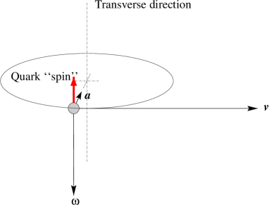
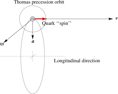
(a)			(b)

Figure 2.11: Thomas precession effect on transversity (a) and helicity (b).

To properly deal with this situation in a relativistic way, we have to take into account Thomas precession, an effect which occurs whenever a frame of reference (in our case joined to the quark) is moving with a velocity $\bm{v}$ with respect to the observer and is at the same time subject to an acceleration $\bm{a}$ [111, 165]. Thomas precession causes the quark frame of reference (and the spin of the quark with it) to precess with an angular velocity

$$\bm{\omega}_{T}=\frac{\bm{v}\times\bm{a}}{2c^{2}}.$$ (2.56)

In the infinite momentum frame, the speed of revolution of the quark is negligible with respect to the overall velocity of the system, so that the quark velocity is approximately $\bm{v}$. However we cannot neglect its centripetal acceleration $\bm{a}$.

Let us first analyze the situation with transversity [Fig. 2.11 (a)]. The cross product of the velocity of the quark and the centripetal acceleration is pointing in the transverse direction. Thomas precession will not influence the orientation of the spin of the quark. The transversity distribution is just 1.

The situation is dramatically different for helicity [Fig. 2.11 (b)]. The cross product of the quark velocity and its acceleration is still pointing in a transverse direction, which is now orthogonal to the spin of the quark. This causes the spin of the quark to precess around a transverse axis. The net helicity of the quark will be zero and so will be the helicity distribution.

In a simpler system, for instance if the quark would not have any orbital angular momentum, helicity and transversity distributions would be the same. In conclusion, from this example we see that, due to relativistic effects, the difference between two apparently similar observables can reveal something important about the structure of a system.

2.4 Inclusion of transverse momentum

So far we have been concerned with the integrated correlation function, defined in Eq. (2.19), the only relevant one in totally inclusive deep inelastic scattering. In the next chapters, we will analyze also semi-inclusive scatterings, where we will need to consider the transverse-momentum dependent version of the correlation function, i.e.

$$\begin{split}\Phi_{ji}(x,\bm{p}_{T},S)&=\int\operatorname{{\rm\,d}}p^{-}\;\Phi_{ji}(p,P,S)\biggr{|}_{p^{+}=xP^{+}}\\ &=\int\frac{\operatorname{{\rm\,d}}\xi^{-}\operatorname{{\rm\,d}}^{2}\!\bm{\xi}_{T}}{(2\pi)^{3}}\;{\rm e}^{-{\rm i}p\cdot\xi}\bigl{\langle}{P,S}\mspace{2.0mu}\raisebox{-3.0pt}{\rule{0.7pt}{12.0pt}}\;\mspace{5.0mu}\makebox[0.0pt]{$\bar{\phantom{\psi}}$}\mspace{-5.0mu}{\psi}\mspace{-5.0mu}\makebox[0.0pt]{$\bar{\phantom{\psi}}$}\mspace{5.0mu}_{i}(\xi)\;\psi_{j}(0)\;\raisebox{-3.0pt}{\rule{0.7pt}{12.0pt}}\,{P,S}\bigr{\rangle}\biggr{|}_{\xi^{+}=0}.\end{split}$$ (2.57)

Starting from the general decomposition presented in Eq. (2.31), the leading order part of the transverse-momentum dependent correlation function becomes

$$\begin{split}{\cal P}_{+}\,\Phi(x,\bm{p}_{T},S)\gamma^{+}&=\Biggl{\{}f_{1}(x,\bm{p}^{2}_{T})+{\rm i}\,h_{1}^{\perp}(x,\bm{p}^{2}_{T})\,\frac{\makebox[0.0pt][l]{\hskip 1.3pt$\sslash$}{p}_{T}}{M}+S_{L}\,g_{1L}(x,\bm{p}^{2}_{T})\,\gamma_{5}+S_{L}\,h_{1L}^{\perp}(x,\bm{p}^{2}_{T})\,\gamma_{5}\,\frac{\makebox[0.0pt][l]{\hskip 1.3pt$\sslash$}{p}_{T}}{M}\\ &\quad+f_{1T}^{\perp}(x,\bm{p}^{2}_{T})\,\frac{\epsilon_{T\rho\sigma}S_{T}^{\rho}p_{T}^{\sigma}}{M}+g_{1T}(x,\bm{p}^{2}_{T})\,\frac{\bm{p}_{T}\cdot\bm{S}_{T}}{M}\,\gamma_{5}\\ &\quad+h_{1T}(x,\bm{p}^{2}_{T})\,\gamma_{5}\,\makebox[0.0pt][l]{\hskip 0.5pt$\sslash$}{S}_{T}+h_{1T}^{\perp}(x,\bm{p}^{2}_{T})\,\frac{\bm{p}_{T}\cdot\bm{S}_{T}}{M}\,\gamma_{5}\,\frac{\makebox[0.0pt][l]{\hskip 1.3pt$\sslash$}{p}_{T}}{M}\Biggr{\}}\,{\cal P}_{+}\,.\end{split}$$ (2.58)

The definition of the parton distribution functions in terms of the amplitudes $A_{i}$, introduced in Eq. (2.33), can be found elsewhere [135, 164, 120].

For any transverse-momentum dependent distribution function, it will turn out to be convenient to define the notation

$$f^{\left(1/2\right)}(x,\bm{p}_{T}^{2}) \equiv\frac{\left\lvert\bm{p}_{T}\right\rvert}{2M}\;f(x,\bm{p}^{2}_{T}),$$ (2.59a)

$$f^{(n)}(x,\bm{p}^{2}_{T}) \equiv\left(\frac{{\bm{p}}_{T}^{2}}{2M^{2}}\right)^{n}f(x,\bm{p}^{2}_{T}),$$ (2.59b)

for $n$ integer. We also need to introduce the function

$$h_{1}(x,\bm{p}^{2}_{T})\equiv h_{1T}(x,\bm{p}^{2}_{T})+h_{1T}^{\perp(1)}(x,\bm{p}^{2}_{T}).$$ (2.60)

The connection with the integrated distribution functions defined in Eq. (2.34) is

$$f_{1}(x) =\int\operatorname{{\rm\,d}}^{2}\!{\bm{p}}_{T}\;f_{1}(x,\bm{p}^{2}_{T}),$$ (2.61a)

$$g_{1}(x) =\int\operatorname{{\rm\,d}}^{2}\!{\bm{p}}_{T}\;g_{1L}(x,\bm{p}^{2}_{T}),$$ (2.61b)

$$h_{1}(x) =\int\operatorname{{\rm\,d}}^{2}\!{\bm{p}}_{T}\;h_{1}(x,\bm{p}^{2}_{T}).$$ (2.61c)

Note that the distribution functions $h_{1}^{\perp}$ and $f_{1T}^{\perp}$ are T-odd. At first, this class of functions was supposed to vanish due to time-reversal invariance [151]. Sivers [157, 158] was the first one to consider an observable arising from the T-odd distribution function $f_{1T}^{\perp}$, since then called the Sivers function. The complete analysis of leading-twist T-odd distribution functions and the introduction of $h_{1}^{\perp}$ were carried out by Boer and Mulders [53]. A proof of the nonexistence of T-odd distribution functions was suggested by Collins in Ref. 77, but recently it has been repudiated by the same author [78] after Brodsky, Hwang and Schmidt [72] explicitly obtained a nonzero Sivers function in the context of a simple model. The question at the moment awaits clarification, but it is likely that T-odd distribution functions will stir a lot of interest in the near future, together with T-odd fragmentation functions, of which we shall abundantly speak in the next chapters.

As done in the previous section, we can express the transverse momentum dependent correlation function as a matrix in the parton chirality space $\otimes$ target helicity space. To simplify the formulae, it is useful to identify the T-odd functions as imaginary parts of some of the T-even functions, which become then complex scalar functions. The following redefinitions are required:

$$g_{1T}+{\rm i}f_{1T}^{\perp} \rightarrow g_{1T}, h_{1L}^{\perp}+{\rm i}h_{1}^{\perp} \rightarrow h_{1L}^{\perp}.$$ (2.62)

The resulting correlation matrix is [32, 33]

$$F(x,\bm{p}_{T})_{\chi^{\phantom{{}^{\prime}}}_{1}\chi^{\prime}_{1}}^{\Lambda_{1}^{\prime}\Lambda^{\phantom{{}^{\prime}}}_{1}}=\left(\begin{array}[]{cc|cc}f_{1}+g_{1L}&\dfrac{|\bm{p}_{T}|}{M}\,{\rm e}^{-{\rm i}\phi_{p}}\,g_{1T}&\dfrac{|\bm{p}_{T}|}{M}\,{\rm e}^{{\rm i}\phi_{p}}\,h_{1L}^{\perp\ast}&2\,h_{1}\\ \dfrac{|\bm{p}_{T}|}{M}\,{\rm e}^{{\rm i}\phi_{p}}\,g_{1T}^{\ast}&f_{1}-g_{1L}&\dfrac{|\bm{p}_{T}|^{2}}{M^{2}}{\rm e}^{2{\rm i}\phi_{p}}\,h_{1T}^{\perp}&-\dfrac{|\bm{p}_{T}|}{M}\,{\rm e}^{{\rm i}\phi_{p}}\,h_{1L}^{\perp}\\[3.0pt] \hline\cr\dfrac{|\bm{p}_{T}|}{M}\,{\rm e}^{-{\rm i}\phi_{p}}\,h_{1L}^{\perp}&\dfrac{|\bm{p}_{T}|^{2}}{M^{2}}{\rm e}^{-2{\rm i}\phi_{p}}\,h_{1T}^{\perp}&f_{1}-g_{1L}&-\dfrac{|\bm{p}_{T}|}{M}\,{\rm e}^{-{\rm i}\phi_{p}}\,g_{1T}^{\ast}\\ 2\,h_{1}&-\dfrac{|\bm{p}_{T}|}{M}\,{\rm e}^{-{\rm i}\phi_{p}}\,h_{1L}^{\perp\ast}&-\dfrac{|\bm{p}_{T}|}{M}\,{\rm e}^{{\rm i}\phi_{p}}\,g_{1T}&f_{1}+g_{1L}\end{array}\right),$$ (2.63)

where for sake of brevity we did not explicitly indicate the $x$ and $\bm{p}_{T}^{2}$ dependence of the distribution functions and where $\phi_{p}$ is the azimuthal angle of the transverse momentum vector.

The distribution matrix is clearly Hermitean. Notice that by introducing the transverse momentum of the quark, the angular momentum conservation requirement becomes less constraining and we can have non zero contributions in all the entries of the scattering matrix. To be more specific, when an exponential ${\rm e}^{{\rm i}l^{\prime}\phi_{p}}$ appears in the matrix, we have to take into account $l^{\prime}$ units of angular momentum in the final state. The condition of angular momentum conservation becomes then $\Lambda^{\prime}_{1}+\chi^{\prime}_{1}+l^{\prime}=\Lambda_{1}+\chi_{1}$. Also the condition of parity conservation is influenced by the presence of orbital angular momentum and becomes

$$F(x,\bm{p}_{T})_{\chi^{\phantom{{}^{\prime}}}_{1}\chi^{\prime}_{1}}^{\Lambda_{1}^{\prime}\Lambda^{\phantom{{}^{\prime}}}_{1}}=(-1)^{l^{\prime}}\,F(x,\bm{p}_{T})_{-\chi^{\phantom{{}^{\prime}}}_{1}\,-\chi^{\prime}_{1}}^{-\Lambda_{1}^{\prime}\,-\Lambda^{\phantom{{}^{\prime}}}_{1}}\biggr{\rvert}_{l^{\prime}\rightarrow-l^{\prime}}.$$ (2.64)

The positivity of the matrix is not hampered by the introduction of the transverse momentum dependence, since

$$\begin{split}F(x,\bm{p}_{T},S)_{\chi^{\phantom{{}^{\prime}}}_{1}\chi^{\prime}_{1}}^{\Lambda_{1}^{\prime}\Lambda^{\phantom{{}^{\prime}}}_{1}}&=\int\frac{\operatorname{{\rm\,d}}\xi^{-}\operatorname{{\rm\,d}}^{2}\!\bm{\xi}_{T}}{(2\pi)^{3}\sqrt{2}}\;{\rm e}^{-{\rm i}p\cdot\xi}\bigl{\langle}{P,\Lambda^{\prime}_{1}}\mspace{2.0mu}\raisebox{-3.0pt}{\rule{0.7pt}{12.0pt}}\;(\psi_{+})^{\dagger}_{\chi_{1}}(\xi)\;(\psi_{+})_{\chi^{\prime}_{1}}(0)\;\raisebox{-3.0pt}{\rule{0.7pt}{12.0pt}}\,{P,\Lambda_{1}}\bigr{\rangle}\biggr{|}_{\xi^{+}=0}\\ &=\frac{1}{\sqrt{2}}\sum_{X}\int\frac{\operatorname{{\rm\,d}}^{3}\!\bm{P}_{X}}{(2\pi)^{3}\,2P_{X}^{0}}\bigl{\langle}{X}\mspace{2.0mu}\raisebox{-3.0pt}{\rule{0.7pt}{12.0pt}}\;(\psi_{+})_{\chi_{1}}(0)\;\raisebox{-3.0pt}{\rule{0.7pt}{12.0pt}}\,{P,\Lambda_{1}^{\prime}}\bigr{\rangle}^{\ast}\bigl{\langle}{X}\mspace{2.0mu}\raisebox{-3.0pt}{\rule{0.7pt}{12.0pt}}\;(\psi_{+})_{\chi^{\prime}_{1}}(0)\;\raisebox{-3.0pt}{\rule{0.7pt}{12.0pt}}\,{P,\Lambda_{1}}\bigr{\rangle}\\ &\quad\times\delta\Bigl{(}\bigl{(}1-x\bigr{)}P^{+}-P^{+}_{X}\Bigr{)}\;\delta^{(2)}\Bigl{(}\bm{p}_{T}-\bm{P}_{X\,T}\Bigr{)}.\end{split}$$ (2.65)

Bounds to insure positivity of any matrix element can be obtained by looking at the one-dimensional and two-dimensional subspaces and at the eigenvalues of the full matrix. The one-dimensional subspaces give the trivial bounds

$$f_{1}(x,\bm{p}_{T}^{2}) \geq 0\,, \left\lvert g_{1L}(x,\bm{p}_{T}^{2})\right\rvert \leq f_{1}(x,\bm{p}_{T}^{2})\,.$$ (2.66)

From the two-dimensional subspaces we get

$$\left\lvert h_{1}\right\rvert \leq\frac{1}{2}\left(f_{1}+g_{1L}\right)\leq f_{1},$$ (2.67a)

$$\left\lvert h_{1T}^{\perp(1)}\right\rvert \leq\frac{1}{2}\left(f_{1}-g_{1L}\right)\leq f_{1},$$ (2.67b)

$$\left\lvert g_{1T}^{(1)}\right\rvert^{2} \leq\frac{\bm{p}_{T}^{2}}{4M^{2}}\left(f_{1}+g_{1L}\right)\left(f_{1}-g_{1L}\right)\leq\left(f_{1}^{(1/2)}\right)^{2},$$ (2.67c)

$$\left\lvert h_{1L}^{\perp(1)}\right\rvert^{2} \leq\frac{\bm{p}_{T}^{2}}{4M^{2}}\left(f_{1}+g_{1L}\right)\left(f_{1}-g_{1L}\right)\leq\left(f_{1}^{(1/2)}\right)^{2},$$ (2.67d)

where, once again, we did not explicitly indicate the $x$ and $\bm{p}_{T}^{2}$ dependence to avoid too heavy a notation. Besides the Soffer bound of Eq. (2.67a), now extended to include the transverse momentum dependence, new bounds for the distribution functions are found.

The positivity bounds can be sharpened even further by imposing the positivity of the eigenvalues of the correlation matrix. The complete analysis has been accomplished in Ref. 32 (see also Ref. 33).

2.5 Cross section and spin asymmetries

The cross section for inclusive deep inelastic scattering at leading twist is expressed by Eq. (2.26). Extracting the target helicity density matrix as done in Eq. (2.43) and using the matrix $F$, the equation becomes

$$\frac{\operatorname{{\rm\,d}}^{3}\!\sigma}{\operatorname{{\rm\,d}}x_{B}\operatorname{{\rm\,d}}y\operatorname{{\rm\,d}}\phi_{S}}\approx\sum_{q}\;\rho(S)_{\Lambda^{\phantom{{}^{\prime}}}_{1}\Lambda_{1}^{\prime}}\;F(x)_{\chi^{\phantom{{}^{\prime}}}_{1}\chi^{\prime}_{1}}^{\Lambda_{1}^{\prime}\Lambda^{\phantom{{}^{\prime}}}_{1}}\Bigl{(}\frac{\operatorname{{\rm\,d}}\sigma^{eq}}{\operatorname{{\rm\,d}}y}\Bigr{)}^{\chi^{\phantom{{}^{\prime}}}_{1}\chi^{\prime}_{1}}\frac{1}{2}.$$ (2.68)

Inserting the expressions of Eq. (2.27), (2.42) and (2.48) into the previous expression leads to the result

$$\frac{\operatorname{{\rm\,d}}^{3}\!\sigma}{\operatorname{{\rm\,d}}x_{B}\operatorname{{\rm\,d}}y\operatorname{{\rm\,d}}\phi_{S}}\approx\frac{2\alpha^{2}}{sx_{B}y^{2}}\,\sum_{q}e_{q}^{2}\,\left[\left(1-y+\frac{y^{2}}{2}\right)f_{1}^{q}(x_{B})+\lambda_{e}\,S_{L}\,\left(y-\frac{y^{2}}{2}\right)\,g_{1}^{q}(x_{B})\right],$$ (2.69)

where the index $q$ denotes the quark flavor.

The transversity distribution does not appear in the cross section for totally inclusive deep inelastic scattering at leading twist. The reason is that it is a chiral odd object and in any observable it must be connected to another chiral odd “probe”. In inclusive deep inelastic scattering, what probes the structure of the correlation function is the elementary photon-quark scattering, which conserves chirality. We will see in the next chapters how semi-inclusive deep inelastic scattering provides the necessary chiral odd partners for the transversity distribution (i.e. chiral odd fragmentation functions).

The r.h.s. of Eq. (2.69) is independent of the azimuthal angle $\phi_{S}$, so that we can integrate the cross section over this angle. The result is

$$\frac{\operatorname{{\rm\,d}}^{2}\!\sigma}{\operatorname{{\rm\,d}}x_{B}\operatorname{{\rm\,d}}y}\approx\frac{4\pi\alpha^{2}}{sx_{B}y^{2}}\,\sum_{q}e_{q}^{2}\,\left[\left(1-y+\frac{y^{2}}{2}\right)f_{1}^{q}(x_{B})+\lambda_{e}S_{L}\,\left(y-\frac{y^{2}}{2}\right)\,g_{1}^{q}(x_{B})\right].$$ (2.70)

If the spin of the target is oriented along the direction of the electron beam, it will have its longitudinal component oriented along the $-z$ direction, that is $S_{L}$ will be negative. On the contrary, orienting the spin of the target in the opposite direction will produce a positive $S_{L}$. Summing the cross sections obtained with opposite polarization, we isolate the unpolarized part of the cross section

$$\operatorname{{\rm\,d}}^{2}\!\sigma_{UU}\equiv\frac{1}{2}\left(\operatorname{{\rm\,d}}^{2}\!\sigma_{\rightarrow\leftarrow}+\operatorname{{\rm\,d}}^{2}\!\sigma_{\rightarrow\rightarrow}\right)\approx\frac{4\pi\alpha^{2}}{sx_{B}y^{2}}\,\left(1-y+\frac{y^{2}}{2}\right)\,\sum_{q}e_{q}^{2}\,f_{1}^{q}(x_{B}).$$ (2.71)

The first subscript indicates the polarization of the beam, while the second stands for the polarization of the target. The letter $U$ stands for unpolarized. The right arrow means polarization along the beam direction, the left arrow means the opposite. Subtracting the cross section we obtain the polarized part

$$\operatorname{{\rm\,d}}^{2}\!\sigma_{LL}\equiv\frac{1}{2}\left(\operatorname{{\rm\,d}}^{2}\!\sigma_{\rightarrow\leftarrow}-\operatorname{{\rm\,d}}^{2}\!\sigma_{\rightarrow\rightarrow}\right)\approx\frac{4\pi\alpha^{2}}{sx_{B}y^{2}}\,\lvert\lambda_{e}\rvert\,\lvert S_{L}\rvert\,\left(y-\frac{y^{2}}{2}\right)\,\sum_{q}e_{q}^{2}\,g_{1}^{q}(x_{B}).$$ (2.72)

where now the subscript $L$ specifies that longitudinal polarizations of beam and target are required. We can define the longitudinal double spin asymmetry

$$A_{LL}(x_{B},y)\equiv\frac{\operatorname{{\rm\,d}}^{2}\!\sigma_{LL}}{\operatorname{{\rm\,d}}^{2}\!\sigma_{UU}}\approx\lvert\lambda_{e}\rvert\,\lvert S_{L}\rvert\,\frac{(1/{x_{B}y^{2}})\,\bigl{(}y-y^{2}/2\bigr{)}\,\sum_{q}e_{q}^{2}\,g_{1}^{q}(x_{B})}{(1/{x_{B}y^{2}})\,\bigl{(}1-y+y^{2}/2\bigr{)}\,\sum_{q}e_{q}^{2}\,f_{1}^{q}(x_{B})}.$$ (2.73)

Note that, since the beam direction does not exactly correspond to the virtual photon direction, the degree of longitudinal polarization of the target will be somewhat smaller than the degree of polarization along the beam direction, while a small transverse polarization will arise [145, 128]. These effects are anyway $1/Q$ suppressed.

2.6 Summary

In this chapter, we introduced the hadronic tensor, containing the information on the structure of hadronic targets in deep inelastic scattering [cf. Eq. (2.6)]. We studied the hadronic tensor in the framework of the parton model at tree level and we came to the introduction of a quark-quark correlation function [cf. Eqs. (2.19) and (2.20)]. The correlation function can be parametrized in terms of parton distribution functions. In particular, at leading order in $1/Q$ (leading twist) we introduced the unpolarized distribution function, $f_{1}$, the helicity distribution function, $g_{1}$, and the transversity distribution function, $h_{1}$ [Eq. (2.33)].

We demonstrated how the leading twist part of the correlation function can be cast in the form of a forward scattering matrix [cf. Eq. (2.48)]. Exploiting the positivity of this matrix, we derived relations among the distribution functions [Eq. (2.49)]. We also discussed the probabilistic interpretation of the distribution function, with a particular emphasis on the transversity distribution.

We repeated the analysis of the correlation function introducing partonic transverse momentum. In this case the decomposition of the correlation function contains eight distribution functions [Eq. (2.58)]. We have seen that each entry of the corresponding scattering matrix is nonzero [Eq. (2.63)], indicating that the full quark spin structure in a polarized nucleon is accessible if transverse momentum is included. The connection with the helicity formalism and consequently the extraction of positivity bounds on transverse momentum dependent distribution functions are among the original results of our work.

Finally, we expressed the cross section for inclusive deep inelastic scattering at leading order in $1/Q$ in terms of distribution functions [Eq. (2.69)]. We showed that the helicity distribution can be accessed by measuring the longitudinal double spin asymmetry, but we concluded that the transversity distribution is not accessible in inclusive deep inelastic scattering.

In the next chapter, we are going to see how the transversity distribution can be measured in one-particle inclusive deep inelastic scattering, in combination with the Collins fragmentation function.

Chapter 3 Fragmentation functions
and the Collins function

In the previous chapter we analyzed totally inclusive deep inelastic scattering as a means to probe the quark structure of the nucleons. We concluded that some aspects of this structure – notably the transversity distribution and the transverse momentum distribution – are not accessible in this kind of measurement. It is therefore desirable to turn the attention to a more complex case, that of one-particle inclusive deep inelastic scattering, where one of the fragments produced in the collision is detected. In this case, we will need to introduce some new nonperturbative objects, the fragmentation functions.

3.1 One-particle inclusive deep inelastic scattering

In one-particle inclusive deep inelastic scattering a high energy electron collides on a target nucleon via the exchange of a photon with a high virtuality. The target breaks up and several hadrons are produced. One of the produced hadrons is detected in coincidence with the scattered electron (see Fig. 3.1). As a result of the hardness of the collision, the final state should consist of two well separated “clusters” of particles, one is represented by the debris of the target, broken by the collision, and the other is represented by the hadrons formed and ejected by the hard interaction with the virtual photon [168]. The former are called target fragments and the latter current fragments. We will take into consideration only events where the tagged final state hadron belongs to the current fragments.

Figure 3.1: One-particle inclusive deep inelastic scattering.

3.1.1 Kinematics

As for inclusive scattering, we denote with $l$ and $l^{\prime}$ the momenta of the electron before and after the scattering, with $P$, $M$ and $S$ the momentum, mass and spin of the target nucleon, with $q$ the momentum of the exchanged photon. Moreover, we introduce the momentum $P_{h}$ and the mass $M_{h}$ of the outgoing hadron.

We define the variables

$$x_{B} =\frac{Q^{2}}{2P\cdot q}, y =\frac{P\cdot q}{P\cdot l}, z_{h} =\frac{P\cdot P_{h}}{P\cdot q}.$$ (3.1)

We will assume that the following conditions hold: $Q^{2},P\cdot q,P\cdot P_{h}\gg M^{2},M_{h}^{2}$, and $x_{B},z_{h}$ fixed.

For a distinction between the current and the target fragments, the rapidity separation should be taken into account. This separation is quite clear for high values of $z_{h}$. For low values of $z_{h}$, separating the two clusters becomes arduous. In events with higher $W^{2}$, the limit of $z_{h}$ can be pushed lower [140].

In the frame of reference defined in Sec. 2.1.1, the target momentum and the virtual photon momentum have no transverse components. The outgoing hadron’s momentum can be parametrized as

$$P_{h}^{\mspace{2.0mu}\mu}=\left[\frac{z_{h}Q}{A\sqrt{2}},\;\frac{A\left(M_{h}^{2}+\lvert\bm{P}_{h\perp}\rvert^{2}\right)}{z_{h}Q\!\sqrt{2}},\;\bm{P}_{h\perp}\right].$$ (3.2)

To avoid the introduction of further hard scales, it is required that $P_{h\perp}^{2}\ll Q^{2}$.

The frame of reference we adopted is the more natural one from the experimental point of view, as the longitudinal direction corresponds (up to order $1/Q$) to the beam direction and the hadron’s transverse momentum corresponds to what it is actually measured in the lab. However, as it will become clear later, in order to preserve a symmetry between the distribution and fragmentation functions, it is convenient to use a different frame of reference where the target and outgoing hadron momenta are collinear, while the photon acquires a transverse component. To distinguish between the two frames of reference when needed, from now on we will use the subscript $T$ when denoting a transverse component in the new frame, while we will use the subscript $\perp$ to denote transverse components in the former frame.

In the $T$ frame, the external momenta are

$$P^{\mspace{2.0mu}\mu} =\left[\frac{x_{B}M^{2}}{AQ\sqrt{2}},\;\frac{AQ}{x_{B}\!\sqrt{2}},\;\bm{0}\right]=\left[\frac{M^{2}}{2P^{+}},\;P^{+},\;\bm{0}\right],$$ (3.3a)

$$P_{h}^{\mspace{2.0mu}\mu} =\left[\frac{z_{h}Q}{A\sqrt{2}},\;\frac{AM_{h}^{2}}{z_{h}Q\!\sqrt{2}},\;\bm{0}\right]=\left[P_{h}^{-},\;\frac{M_{h}^{2}}{2P_{h}^{-}},\;{\bf 0}\right],$$ (3.3b)

$$q^{\mspace{2.0mu}\mu} =\left[\frac{Q}{A\sqrt{2}},\;-\frac{A\,\left(Q^{2}-\lvert\bm{q}_{T}\rvert^{2}\right)}{Q\sqrt{2}},\;\bm{q}_{T}\right]\approx\left[\frac{P_{h}^{-}}{z_{h}},\;-x_{B}P^{+},\;\bm{q}_{T}\right],$$ (3.3c)

with $P_{h}^{-}\approx Q^{2}z_{h}/(2P^{+}x_{B})$. The connection with the transverse momentum components of the photon in the $T$ frame and of the outgoing hadron in the $\perp$ frame is [141]

$$\bm{q}_{T}=-\frac{\bm{P}_{h\perp}}{z_{h}}.$$ (3.4)

3.1.2 The hadronic tensor

The cross section for one-particle inclusive electron-nucleon scattering can be written as

$$\frac{2E_{h}\operatorname{{\rm\,d}}^{6}\!\sigma}{\operatorname{{\rm\,d}}^{3}\!\bm{P}_{h}\operatorname{{\rm\,d}}x_{B}\operatorname{{\rm\,d}}y\operatorname{{\rm\,d}}\phi_{S}}=\frac{\alpha^{2}}{2sx_{B}Q^{2}}\,L_{\mu\nu}(l,l^{\prime},\lambda_{e})\,2MW^{\mu\nu}(q,P,S,P_{h}),$$ (3.5)

or equivalently as

$$\frac{\operatorname{{\rm\,d}}^{6}\!\sigma}{\operatorname{{\rm\,d}}x_{B}\operatorname{{\rm\,d}}y\operatorname{{\rm\,d}}z_{h}\operatorname{{\rm\,d}}\phi_{S}\operatorname{{\rm\,d}}^{2}\!\bm{P}_{h\perp}}=\frac{\alpha^{2}}{4z_{h}sx_{B}Q^{2}}\,L_{\mu\nu}(l,l^{\prime},\lambda_{e})\;2MW^{\mu\nu}(q,P,S,P_{h}).$$ (3.6)

To obtain the previous formula, we made use of the relation $\operatorname{{\rm\,d}}^{3}\!P_{h}/2E_{h}\approx\operatorname{{\rm\,d}}z_{h}\operatorname{{\rm\,d}}^{2}\!\bm{P}_{h\perp}/2z_{h}$.

The hadronic tensor for one-particle inclusive scattering is defined as

$$2MW^{\mu\nu}(q,P,S,P_{h}) =\frac{1}{(2\pi)^{4}}\sum_{\cal X^{\prime}}\int\frac{\operatorname{{\rm\,d}}^{3}\!\bm{P}_{\cal X^{\prime}}}{2P_{\cal X^{\prime}}^{0}}\;2\pi\,\delta^{(4)}\Bigl{(}q+P-P_{\cal X^{\prime}}-P_{h}\Bigr{)}\,H^{\mu\nu}(P,S,P_{\cal X^{\prime}},P_{h}),$$ (3.7)

$$H^{\mu\nu}(P,S,P_{\cal X^{\prime}},P_{h}) =\bigl{\langle}{P,S}\mspace{2.0mu}\raisebox{-3.0pt}{\rule{0.7pt}{12.0pt}}\;J^{\mu}(0)\;\raisebox{-3.0pt}{\rule{0.7pt}{12.0pt}}\,{P_{h},{\cal X^{\prime}}}\bigr{\rangle}\bigl{\langle}{P_{h},{\cal X^{\prime}}}\mspace{2.0mu}\raisebox{-3.0pt}{\rule{0.7pt}{12.0pt}}\;J^{\nu}(0)\;\raisebox{-3.0pt}{\rule{0.7pt}{12.0pt}}\,{P,S}\bigr{\rangle}.$$ (3.8)

By integrating over the momentum of the final-state hadron and summing over all possible hadrons, we recover the hadronic tensor for totally inclusive scattering

$$\begin{split}\sum_{h}\int\frac{\operatorname{{\rm\,d}}^{3}\!P_{h}}{2P_{h}^{0}}\;2MW^{\mu\nu}(q,P,S,P_{h})&=\frac{1}{2\pi}\sum_{\cal X}\int\frac{\operatorname{{\rm\,d}}^{3}\!P_{\cal X}}{2P_{\cal X}^{0}}\;2\pi\,\delta^{(4)}\Bigl{(}q+P-P_{\cal X}\Bigr{)}\,H^{\mu\nu}(P,S,P_{\cal X})\\ &\equiv 2MW^{\mu\nu}(q,P,S),\end{split}$$ (3.9)

where now the state $\cal X$ indicates the sum of the states $\cal X^{\prime}$ and $h$, and $P_{\cal X}=P_{\cal X^{\prime}}+P_{h}$. Note that we did not include any dependence of the hadronic tensor on the polarization of the final state hadron. The reason is that this polarization is usually measured through the decay of the final state hadron into other hadrons. In this sense, this case falls within the context of two-particle (or even three-particle) inclusive scattering, as we will show in the next chapter.

In the spirit of the parton model, the virtual photon strikes a quark inside the nucleon. In the case of current fragmentation, the tagged final state hadron comes from the fragmentation of the struck quark. The scattering process can then be factorized in two soft hadronic parts connected by a hard scattering part, as shown in Fig. 3.2.

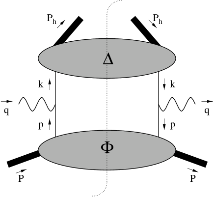
Figure 3.2: The bull diagram, describing the hadronic tensor at tree level.

We need to introduce a parametrization for the vectors

$$p^{\mspace{2.0mu}\mu} =\left[\frac{p^{2}+|\bm{p}_{T}|^{2}}{2xP^{+}},\;xP^{+},\;\bm{p}_{T}\right],$$ (3.10a)

$$k^{\mspace{2.0mu}\mu} =\left[\frac{P_{h}^{-}}{z},\;\frac{z\left(k^{2}+|\bm{k}_{T}|^{2}\right)}{2P_{h}^{-}},\;\bm{k}_{T}\right].$$ (3.10b)

Without expliciting including the antiquark contributions, the hadronic tensor can be written at tree level as

$$2MW^{\mu\nu}(q,P,S,P_{h})=\sum_{q}e_{q}^{2}\int\operatorname{{\rm\,d}}^{4}\!p\operatorname{{\rm\,d}}^{4}\!k\;\delta^{(4)}\left(p+q-k\right)\,\operatorname{Tr}\left(\Phi(p,P,S)\,\gamma^{\mspace{2.0mu}\mu}\,\Delta(k,P_{h})\,\gamma^{\nu}\right),$$ (3.11)

where $\Phi$ is the correlation function defined in Eq. (2.16a) and $\Delta$,

$$\begin{split}\Delta_{kl}(k,P_{h})&=\frac{1}{(2\pi)^{4}}\int\operatorname{{\rm\,d}}^{4}\!\xi\;{\rm e}^{{\rm i}k\cdot\xi}\,\bigl{\langle}{0}\mspace{2.0mu}\raisebox{-3.0pt}{\rule{0.7pt}{12.0pt}}\;\psi_{k}(\xi)\;\raisebox{-3.0pt}{\rule{0.7pt}{12.0pt}}\,{P_{h}}\bigr{\rangle}\bigl{\langle}{P_{h}}\mspace{2.0mu}\raisebox{-3.0pt}{\rule{0.7pt}{12.0pt}}\;\mspace{5.0mu}\makebox[0.0pt]{$\bar{\phantom{\psi}}$}\mspace{-5.0mu}{\psi}\mspace{-5.0mu}\makebox[0.0pt]{$\bar{\phantom{\psi}}$}\mspace{5.0mu}_{l}(0)\;\raisebox{-3.0pt}{\rule{0.7pt}{12.0pt}}\,{0}\bigr{\rangle}\\ &=\sum_{Y}\int\frac{\operatorname{{\rm\,d}}^{3}\!\bm{P}_{Y}}{(2\pi)^{3}\,2P_{Y}^{0}}\;\bigl{\langle}{0}\mspace{2.0mu}\raisebox{-3.0pt}{\rule{0.7pt}{12.0pt}}\;\psi_{k}(0)\;\raisebox{-3.0pt}{\rule{0.7pt}{12.0pt}}\,{P_{h},Y}\bigr{\rangle}\bigl{\langle}{P_{h},Y}\mspace{2.0mu}\raisebox{-3.0pt}{\rule{0.7pt}{12.0pt}}\;\mspace{5.0mu}\makebox[0.0pt]{$\bar{\phantom{\psi}}$}\mspace{-5.0mu}{\psi}\mspace{-5.0mu}\makebox[0.0pt]{$\bar{\phantom{\psi}}$}\mspace{5.0mu}_{l}(0)\;\raisebox{-3.0pt}{\rule{0.7pt}{12.0pt}}\,{0}\bigr{\rangle}\;\delta^{(4)}\Bigl{(}k-P_{h}-P_{Y}\Bigr{)},\end{split}$$ (3.12)

is a new correlation function we need to introduce to describe the fragmentation process [81].

Neglecting terms which are $1/Q$ suppressed, we obtain the compact expression

$$2MW^{\mu\nu}(q,P,S,P_{h})=4z_{h}\,{\cal I}\Bigl{[}\operatorname{Tr}{\left(\Phi(x_{B},\bm{p}_{T},S)\,\gamma^{\mspace{2.0mu}\mu}\,\Delta(z_{h},\bm{k}_{T})\,\gamma^{\nu}\right)}\Bigr{]},$$ (3.13)

where, as we shall do very often, we used the shorthand notation

$${\cal I}\Bigl{[}\dotsb\Bigr{]}\equiv\int\operatorname{{\rm\,d}}^{2}\!\bm{p}_{T}\operatorname{{\rm\,d}}^{2}\bm{k}_{T}\,\delta^{(2)}\Bigl{(}\bm{p}_{T}+\bm{q}_{T}-\bm{k}_{T}\Bigr{)}\;\Bigl{[}\dotsb\Bigr{]}=\int\operatorname{{\rm\,d}}^{2}\!\bm{p}_{T}\operatorname{{\rm\,d}}^{2}\bm{k}_{T}\,\delta^{(2)}\Bigl{(}\bm{p}_{T}-\frac{\bm{P}_{h\perp}}{z}-\bm{k}_{T}\Bigr{)}\;\Bigl{[}\dotsb\Bigr{]},$$ (3.14)

and where we introduced the integrated correlation functions

$$\Phi(x,\bm{p}_{T},S) \equiv\int\operatorname{{\rm\,d}}p^{-}\Phi(p,P,S)\Bigr{|}_{p^{+}=xP^{+}},$$ (3.15a)

$$\Delta(z,\bm{k}_{T}) \equiv\frac{1}{4z}\int\operatorname{{\rm\,d}}k^{+}\Delta(k,P_{h})\Bigr{|}_{k^{-}=P_{h}^{-}/z}.$$ (3.15b)

Often in experimental situations the transverse momentum of the outgoing hadron is not measured. This corresponds to integrating over the outgoing hadron’s transverse momentum, $\bm{P}_{h\perp}$. As we already pointed out, this transverse momentum squared has to be small compared to $Q^{2}$. Experimentally, this can be insured by imposing a cut-off on the data. Due to the $\delta$ distribution in Eq. (3.14), this condition implies also $(\bm{p}_{T}+\bm{k}_{T})^{2}\ll Q^{2}$. Considerations as the one discussed in Sec. 2.1.2, can be applied to the perturbative and intrinsic components of the transverse momenta.

The integration of the cross section yields

$$\frac{\operatorname{{\rm\,d}}^{4}\!\sigma}{\operatorname{{\rm\,d}}x_{B}\operatorname{{\rm\,d}}y\operatorname{{\rm\,d}}z_{h}\operatorname{{\rm\,d}}\phi_{S}}=\frac{\alpha^{2}}{4z_{h}sx_{B}\,Q^{2}}\,L_{\mu\nu}(l,l^{\prime},\lambda_{e})\;2MW^{\mu\nu}(q,P,S),$$ (3.16)

where

$$2MW^{\mu\nu}(q,P,S) =4z_{h}\,\operatorname{Tr}{\left(\Phi(x_{B},S)\,\gamma^{\mspace{2.0mu}\mu}\,\Delta(z_{h})\,\gamma^{\nu}\right)},$$ (3.17a)

$$\Phi(x,S) \equiv\int\operatorname{{\rm\,d}}p^{-}\operatorname{{\rm\,d}}^{2}\!\bm{p}_{T}\,\Phi(p,P,S)\Bigr{|}_{p^{+}=xP^{+}},$$ (3.17b)

$$\Delta(z) \equiv\frac{z}{4}\int\operatorname{{\rm\,d}}k^{+}\operatorname{{\rm\,d}}^{2}\!\bm{k}_{T}\,\Delta(k,P_{h})\Bigr{|}_{k^{-}=P_{h}^{-}/z}.$$ (3.17c)

3.1.3 Leading twist part and connection with helicity formalism

Using the projectors $\cal P_{+}$ and $\cal P_{-}$ defined in Eq. (2.23), we can isolate the leading order part of the hadronic tensor, analogously to what was done in Sec. 2.1.4

$$\begin{split}2MW^{\mu\nu}(q,P,S,P_{h})&\approx 4z_{h}\,{\cal I}\Biggl{[}\operatorname{Tr}{\left({\cal P}_{+}\,\Phi(x_{B},\bm{p}_{T},S)\;{\cal P}_{-}\;\gamma^{\mspace{2.0mu}\mu}\;{\cal P}_{-}\,\Delta(z_{h},\bm{k}_{T})\;{\cal P}_{+}\;\gamma^{\nu}\right)}\Biggr{]}\\ &=4z_{h}\,{\cal I}\left[\operatorname{Tr}{\left({\cal P}_{+}\,\Phi(x_{B},\bm{p}_{T},S)\,\gamma^{+}\;\frac{\gamma^{-}\gamma^{\mspace{2.0mu}\mu}}{2}\,{\cal P}_{-}\;{\cal P}_{-}\,\Delta(z_{h},\bm{k}_{T})\,\gamma^{-}\;\frac{\gamma^{+}\gamma^{\nu}}{2}\,{\cal P}_{+}\right)}\right].\end{split}$$ (3.18)

The differential cross section becomes

$$\begin{split}\@ADDCLASS{ltx_eqn_lefteqn}$\displaystyle\frac{\operatorname{{\rm\,d}}^{6}\!\sigma}{\operatorname{{\rm\,d}}x_{B}\operatorname{{\rm\,d}}y\operatorname{{\rm\,d}}z_{h}\operatorname{{\rm\,d}}\phi_{S}\operatorname{{\rm\,d}}^{2}\!\bm{P}_{h\perp}}$\mbox{}\hfil\\ &\approx\sum_{q}\,\frac{\alpha^{2}e_{q}^{2}}{sx_{B}Q^{2}}\,L_{\mu\nu}(l,l^{\prime},\lambda_{e})\;{\cal I}\left[\operatorname{Tr}{\left({\cal P}_{+}\,\Phi(x_{B},\bm{p}_{T},S)\,\gamma^{+}\;\frac{\gamma^{-}\gamma^{\mspace{2.0mu}\mu}}{2}\,{\cal P}_{-}\;{\cal P}_{-}\,\Delta(z_{h},\bm{k}_{T})\,\gamma^{-}\;\frac{\gamma^{+}\gamma^{\nu}}{2}\,{\cal P}_{+}\right)}\right]\\ &\approx\sum_{q}\,{\cal I}\left[\Bigl{(}{\cal P}_{+}\,\Phi(x_{B},\bm{p}_{T},S)\gamma^{+}\Bigr{)}_{ij}\;\frac{\alpha^{2}e_{q}^{2}}{sx_{B}Q^{2}}\,L_{\mu\nu}(l,l^{\prime},\lambda_{e})\left(\frac{\gamma^{-}\gamma^{\mspace{2.0mu}\mu}}{2}\,{\cal P}_{-}\right)_{jl}\left(\frac{\gamma^{+}\gamma^{\nu}}{2}\,{\cal P}_{+}\right)_{mi}\Bigl{(}{\cal P}_{-}\,\Delta(z_{h},\bm{k}_{T})\,\gamma^{-}\Bigr{)}_{lm}\right].\end{split}$$ (3.19)

As we already discussed in Sec. 2.2.1, the restriction to the leading order allows us to reduce the four dimensional Dirac space to the two-dimensional subspace of good fields. Writing all the components of the cross section in the chirality space of the good fields, we obtain

$$\begin{split}\frac{\operatorname{{\rm\,d}}^{6}\!\sigma}{\operatorname{{\rm\,d}}x_{B}\operatorname{{\rm\,d}}y\operatorname{{\rm\,d}}z_{h}\operatorname{{\rm\,d}}\phi_{S}\operatorname{{\rm\,d}}^{2}\!\bm{P}_{h\perp}}&=\rho(S)_{\Lambda^{\phantom{{}^{\prime}}}_{1}\Lambda_{1}^{\prime}}\;{\cal I}\left[\Bigl{(}{\cal P}_{+}\,\Phi(x_{B},\bm{p}_{T})\gamma^{+}\Bigr{)}_{\chi^{\prime}_{1}\chi^{\phantom{{}^{\prime}}}_{1}}^{\Lambda_{1}^{\prime}\Lambda^{\phantom{{}^{\prime}}}_{1}}\Bigl{(}\frac{\operatorname{{\rm\,d}}\sigma^{eq}}{\operatorname{{\rm\,d}}y}\Bigr{)}^{\chi^{\phantom{{}^{\prime}}}_{1}\chi^{\prime}_{1};\,\chi^{\phantom{{}^{\prime}}}_{2}\chi^{\prime}_{2}}\Bigl{(}{\cal P}_{-}\,\Delta(z_{h})\,\gamma^{-}\Bigr{)}_{\chi^{\prime}_{2}\chi^{\phantom{{}^{\prime}}}_{2}}\right]\\ &\equiv\rho(S)_{\Lambda^{\phantom{{}^{\prime}}}_{1}\Lambda_{1}^{\prime}}\;{\cal I}\left[F(x_{B},\bm{p}_{T})_{\chi^{\phantom{{}^{\prime}}}_{1}\chi^{\prime}_{1}}^{\Lambda_{1}^{\prime}\Lambda^{\phantom{{}^{\prime}}}_{1}}\Bigl{(}\frac{\operatorname{{\rm\,d}}\sigma^{eq}}{\operatorname{{\rm\,d}}y}\Bigr{)}^{\chi^{\phantom{{}^{\prime}}}_{1}\chi^{\prime}_{1};\,\chi^{\phantom{{}^{\prime}}}_{2}\chi^{\prime}_{2}}D(z_{h},\bm{k}_{T})_{\chi^{\prime}_{2}\chi^{\phantom{{}^{\prime}}}_{2}}\right].\end{split}$$ (3.20)

The elementary electron-quark scattering matrix is

$$\begin{split}\Bigl{(}\frac{\operatorname{{\rm\,d}}\sigma^{eq}}{\operatorname{{\rm\,d}}y}\Bigr{)}^{\chi^{\phantom{{}^{\prime}}}_{1}\chi^{\prime}_{1};\,\chi^{\phantom{{}^{\prime}}}_{2}\chi^{\prime}_{2}}&=\frac{\alpha^{2}e_{q}^{2}}{sx_{B}Q^{2}}\,L_{\mu\nu}(l,l^{\prime},\lambda_{e})\left(\frac{\gamma^{-}\gamma^{\mspace{2.0mu}\mu}}{2}\,{\cal P}_{-}\right)^{\chi^{\phantom{{}^{\prime}}}_{1}\chi^{\phantom{{}^{\prime}}}_{2}}\left(\frac{\gamma^{+}\gamma^{\nu}}{2}\,{\cal P}_{+}\right)^{\chi^{\prime}_{2}\chi^{\prime}_{1}}\\[8.53581pt] &=\frac{2\alpha^{2}e_{q}^{2}}{sx_{B}y^{2}}\,\left(\begin{array}[]{cc|cc}A(y)+\lambda_{e}C(y)&0&0&-B(y)\\ 0&0&0&0\\ \hline\cr 0&0&0&0\\ -B(y)&0&0&A(y)-\lambda_{e}C(y)\end{array}\right),\end{split}$$ (3.21)

where

$$A(y) =1-y+\frac{y^{2}}{2}, B(y) =(1-y), C(y) =y\left(1-\frac{y}{2}\right).$$ (3.22)

The internal blocks have indices $\chi^{\prime}_{1}\;\chi^{\phantom{{}^{\prime}}}_{1}$ and the outer matrix has indices $\chi^{\prime}_{2}\;\chi^{\phantom{{}^{\prime}}}_{2}$. Notice the difference between Eq. (3.21) and Eq. (2.27): in the latter, the presence of the Kronecker delta was identifying two of the chirality indices, thus reproducing a true scattering matrix. Here, we don’t have just a quark line connecting the two scattering amplitudes, but rather the correlation function $\Delta$. For this reason, we cannot identify the chirality indices of the outgoing quark. Strictly speaking, this is not a scattering matrix anymore, but a scattering amplitude times the conjugate of a different scattering amplitude [19]. However, for conciseness we follow the notation of, e.g., Ref. 117.

The leading order part of the correlation function corresponds to the transition probability density for the process of a quark decaying into hadrons

$$\begin{split}\Bigl{(}{\cal P}_{-}\,\Delta(z,\bm{k}_{T})\,\gamma^{-}\Bigr{)}_{\chi^{\prime}_{2}\chi^{\phantom{{}^{\prime}}}_{2}}\equiv D(z,\bm{k}_{T})_{\chi^{\prime}_{2}\chi^{\phantom{{}^{\prime}}}_{2}}&=\int\frac{\operatorname{{\rm\,d}}\xi^{+}\operatorname{{\rm\,d}}^{2}\!\bm{\xi}_{T}}{(2\pi)^{3}\sqrt{2}}\;{\rm e}^{{\rm i}k\cdot\xi}\bigl{\langle}{0}\mspace{2.0mu}\raisebox{-3.0pt}{\rule{0.7pt}{12.0pt}}\;(\psi_{-})_{\chi^{\prime}_{2}}(\xi)\;\raisebox{-3.0pt}{\rule{0.7pt}{12.0pt}}\,{P_{h}}\bigr{\rangle}\bigl{\langle}{P_{h}}\mspace{2.0mu}\raisebox{-3.0pt}{\rule{0.7pt}{12.0pt}}\;(\psi_{-})^{\dagger}_{\chi_{2}}(0)\;\raisebox{-3.0pt}{\rule{0.7pt}{12.0pt}}\,{0}\bigr{\rangle}\biggr{|}_{\xi^{-}=0}\\ &=\frac{1}{\sqrt{2}}\sum_{Y}\int\frac{\operatorname{{\rm\,d}}^{3}\!\bm{P}_{Y}}{(2\pi)^{3}\,2P_{Y}^{0}}\;\bigl{\langle}{0}\mspace{2.0mu}\raisebox{-3.0pt}{\rule{0.7pt}{12.0pt}}\;(\psi_{-})_{\chi^{\prime}_{2}}(0)\;\raisebox{-3.0pt}{\rule{0.7pt}{12.0pt}}\,{P_{h},Y}\bigr{\rangle}\bigl{\langle}{0}\mspace{2.0mu}\raisebox{-3.0pt}{\rule{0.7pt}{12.0pt}}\;(\psi_{-})_{\chi_{2}}(0)\;\raisebox{-3.0pt}{\rule{0.7pt}{12.0pt}}\,{P_{h},Y}\bigr{\rangle}^{\ast}\\ &\quad\times\delta\Bigl{(}\bigl{(}1/z-1\bigr{)}P_{h}^{-}-P^{-}_{Y}\Bigr{)}\;\delta^{(2)}\left(\bm{k}_{T}-\bm{P}_{YT}\right).\end{split}$$ (3.23)

Analogously to the distribution case, the fragmentation correlation matrix is positive semidefinite, allowing us to set bounds on the fragmentation functions.

3.2 The correlation function $\Delta$

While the distribution correlation function describe the confinement of partons inside hadrons, the fragmentation correlation function describes the way a virtual parton “decays” into a hadron plus something else, i.e. $q^{*}\rightarrow hY$. This process is referred to as hadronization. It is a clear manifestation of color confinement: the asymptotic physical states detected in experiment must be color neutral, so that quarks have to evolve into hadrons. Nowadays, we can count on reliable phenomenological descriptions of hadronization, such as the Lund model. On the other side, understanding it from first principles, as well as including spin degrees of freedom, is very difficult.

As on the distribution side the quark-quark correlation function is sufficient to describe the dynamics at leading order in $1/Q$, also for fragmentation it is sufficient to consider quark-quark correlation functions.

The procedure for generating a complete decomposition of the correlation functions closely follows what has been done on the distribution side in Sec. 2.2. It is necessary to combine the Lorentz vectors $k$ and $P_{h}$ with a basis of structures in Dirac space, and impose the condition of Hermiticity and parity invariance. The outcome is

$$\Delta(k,P_{h})=M_{h}\,B_{1}\,{\bm{1}}+B_{2}\,\makebox[0.0pt][l]{\hskip 1.2pt$\sslash$}{P}_{h}+B_{3}\,\makebox[0.0pt][l]{$\sslash$}{k}+\frac{B_{4}}{M_{h}}\,\sigma_{\mu\nu}P_{h}^{\mspace{2.0mu}\mu}k^{\nu}.$$ (3.24)

The amplitudes $B_{i}$ are dimensionless real scalar functions $B_{i}=B_{i}(k\cdot P_{h},k^{2})$. The T-even and T-odd part of the correlation function $\Delta$ can be defined in analogy to Eqs. (2.32). According to those definitions, the last term can be classified as T-odd.

At leading twist, we are interested in the projection ${\cal P}_{-}\,\Delta(z,\bm{k}_{T})\,\gamma^{-}$. The insertion of the decomposition given in Eq. (3.24) into Eq. (3.15b) and the subsequent projection of the leading-twist component leads to

$${\cal P}_{-}\,\Delta(z,\bm{k}_{T})\,\gamma^{-}=\frac{1}{2}\left(D_{1}(z,z^{2}\bm{k}^{2}_{T})+i\,H_{1}^{\perp}(z,z^{2}\bm{k}^{2}_{T})\,\frac{\makebox[0.0pt][l]{$\sslash$}{k}_{T}}{M_{h}}\right){\cal P}_{-}\,,$$ (3.25)

where we introduced the parton fragmentation functions

$$D_{1}(z,z^{2}\bm{k}_{T}^{2}) =\frac{1}{2z}\int\operatorname{{\rm\,d}}k^{2}\operatorname{{\rm\,d}}(2k\cdot P_{h})\;\delta\left(\bm{k}_{T}^{2}+\frac{M_{h}^{2}}{z^{2}}+k^{2}-\frac{2k\cdot P_{h}}{z}\right)\;\left[B_{2}+\frac{1}{z}B_{3}\right],$$ (3.26a)

$$H_{1}^{\perp}(z,z^{2}\bm{k}_{T}^{2}) =\frac{1}{2z}\int\operatorname{{\rm\,d}}k^{2}\operatorname{{\rm\,d}}(2k\cdot P_{h})\;\delta\left(\bm{k}_{T}^{2}+\frac{M_{h}^{2}}{z^{2}}+k^{2}-\frac{2k\cdot P_{h}}{z}\right)\;\left[-B_{4}\right].$$ (3.26b)

The fragmentation function $H_{1}^{\perp}$ is known with the name of Collins function [77].

The individual fragmentation functions can be isolated by means of the projection

$$\Delta^{[\Gamma]}\equiv\operatorname{Tr}\left(\Delta\Gamma\right),$$ (3.27)

where $\Gamma$ stands for a specific Dirac structure. In particular, we see that

$$D_{1}(z,z^{2}\bm{k}_{T}^{2}) =\Delta^{[\gamma^{-}]}(z,\bm{k}_{T}),$$ (3.28a)

$$\frac{\epsilon_{T}^{ij}k_{T\,j}}{M_{h}}H_{1}^{\perp}(z,z^{2}\bm{k}_{T}^{2}) =\Delta^{[{\rm i}\sigma^{i-}\gamma_{5}]}(z,\bm{k}_{T}).$$ (3.28b)

As we have done with the distribution functions, it will be helpful to introduce the notation

$$D^{\left(1/2\right)}(z,z^{2}\bm{k}^{2}_{T}) \equiv\frac{\left\lvert\bm{k}_{T}\right\rvert}{2M_{h}}\;D(z,z^{2}\bm{k}^{2}_{T}),$$ (3.29a)

$$D^{(n)}(z,z^{2}\bm{k}^{2}_{T}) \equiv\left(\frac{{\bm{k}}_{T}^{2}}{2M_{h}^{2}}\right)^{n}D(z,z^{2}\bm{k}^{2}_{T}),$$ (3.29b)

for $n$ integer.

3.2.1 Correlation function in helicity formalism

Expressing the Dirac matrices of Eq. (3.25) in the chiral or Weyl representation, as done in Sec. 2.2.1, we get for the leading twist part of the correlation function the expression

$$\Bigl{(}{\cal P}_{-}\,\Delta(z,\bm{k}_{T})\,\gamma^{-}\Bigr{)}_{kl}=\frac{1}{2}\begin{pmatrix}0&0&0&0\\ 0&D_{1}(z,z^{2}\bm{k}_{T}^{2})&{\rm i}{\rm e}^{{\rm i}\phi_{k}}\,\dfrac{\left\lvert\bm{k}_{T}\right\rvert}{M_{h}}\,H_{1}^{\perp}(z,z^{2}\bm{k}_{T}^{2})&0\\ 0&-{\rm i}{\rm e}^{-{\rm i}\phi_{k}}\,\dfrac{\left\lvert\bm{k}_{T}\right\rvert}{M_{h}}\,H_{1}^{\perp}(z,z^{2}\bm{k}_{T}^{2})&D_{1}(z,z^{2}\bm{k}_{T}^{2})&0\\ 0&0&0&0\end{pmatrix}.$$ (3.30)

Restricting ourselves to the subspace of good quark fields and using the chirality basis, we can rewrite the correlation function as

$$D(z,\bm{k}_{T})_{\chi^{\prime}_{2}\chi^{\phantom{{}^{\prime}}}_{2}}=\frac{1}{2}\begin{pmatrix}D_{1}(z,z^{2}\bm{k}_{T}^{2})&{\rm i}{\rm e}^{{\rm i}\phi_{k}}\,\dfrac{\left\lvert\bm{k}_{T}\right\rvert}{M_{h}}\,H_{1}^{\perp}(z,z^{2}\bm{k}_{T}^{2})\\ -{\rm i}{\rm e}^{-{\rm i}\phi_{k}}\,\dfrac{\left\lvert\bm{k}_{T}\right\rvert}{M_{h}}\,H_{1}^{\perp}(z,z^{2}\bm{k}_{T}^{2})&D_{1}(z,z^{2}\bm{k}_{T}^{2})\end{pmatrix}.$$ (3.31)

Fig. 3.3 shows diagrammatically the position of the indices of the correlation function.

Figure 3.3: Illustration of the position of the indices of the correlation matrix.

Besides being Hermitean, the matrix fulfills the properties of angular momentum conservation and parity invariance. Because of the presence of factors ${\rm e}^{{\rm i}l\phi_{k}}$, we have to take into account $l$ units of angular momentum in the initial state, therefore the condition of angular momentum conservation is $\chi^{\prime}_{2}=\chi_{2}+l$ and the condition of parity invariance is

$$D(z,\bm{k}_{T})_{\chi^{\prime}_{2}\chi^{\phantom{{}^{\prime}}}_{2}}=(-1)^{l}\,D(z,\bm{k}_{T})_{-\chi^{\prime}_{2}\;-\chi^{\phantom{{}^{\prime}}}_{2}}\Bigr{\rvert}_{l\rightarrow-l}.$$ (3.32)

Positivity of the correlation matrix implies the bounds

$$D_{1}(z,z^{2}\bm{k}_{T}^{2}) \geq 0,$$ (3.33a)

$$\left\lvert H_{1}^{\perp(1)}(z,z^{2}\bm{k}_{T}^{2})\right\rvert \leq D_{1}^{(1/2)}(z,z^{2}\bm{k}_{T}^{2}).$$ (3.33b)

3.3 Cross section and asymmetries

In order to obtain the cross section for one-particle inclusive deep inelastic scattering, the expressions for the spin density matrix of the target, Eq. (2.42), for the distribution correlation matrix, Eq. (2.48), and for the fragmentation correlation matrix Eq. (3.31) have to be inserted in the formula for the cross section

$$\frac{\operatorname{{\rm\,d}}^{6}\!\sigma}{\operatorname{{\rm\,d}}x_{B}\operatorname{{\rm\,d}}y\operatorname{{\rm\,d}}z_{h}\operatorname{{\rm\,d}}\phi_{S}\operatorname{{\rm\,d}}^{2}\!\bm{P}_{h\perp}}=\sum_{q}\,\rho(S)_{\Lambda^{\phantom{{}^{\prime}}}_{1}\Lambda_{1}^{\prime}}\;{\cal I}\left[F(x_{B},\bm{p}_{T})_{\chi^{\phantom{{}^{\prime}}}_{1}\chi^{\prime}_{1}}^{\Lambda_{1}^{\prime}\Lambda^{\phantom{{}^{\prime}}}_{1}}\Bigl{(}\frac{\operatorname{{\rm\,d}}\sigma^{eq}}{\operatorname{{\rm\,d}}y}\Bigr{)}^{\chi^{\phantom{{}^{\prime}}}_{1}\chi^{\prime}_{1};\,\chi^{\phantom{{}^{\prime}}}_{2}\chi^{\prime}_{2}}D(z_{h},\bm{k}_{T})_{\chi^{\prime}_{2}\chi^{\phantom{{}^{\prime}}}_{2}}\right].$$ (3.34)

Instead of presenting the full cross section, we turn directly to sum and differences of polarized cross sections. As in the previous chapter, we will use the symbols $\rightarrow$ to indicate polarization along the beam direction and $\leftarrow$ opposite to it. We will also use $\uparrow$ to indicate transverse polarization in the direction specified by the angle $\phi_{S}$, and $\downarrow$ opposite to it. The subscript $U$ will denote unpolarized particles, while $L$ and $T$ will denote longitudinally and transversely polarized particles. The first subscript describes always the beam polarization and the second subscript the target polarization. Fig. 3.4 gives a pictorial description of the vectors and angles involved in one-particle inclusive deep inelastic scattering.

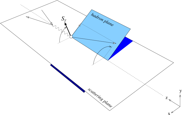
Figure 3.4: Description of the vectors and angles involved in one-particle inclusive deep inelastic scattering.

The unpolarized cross section reads [57]

$$\frac{\operatorname{{\rm\,d}}^{6}\!\sigma_{UU}}{\operatorname{{\rm\,d}}x_{B}\operatorname{{\rm\,d}}y\operatorname{{\rm\,d}}z_{h}\operatorname{{\rm\,d}}\phi_{S}\operatorname{{\rm\,d}}^{2}\!\bm{P}_{h\perp}}=\frac{2\alpha^{2}}{sx_{B}y^{2}}\,\Biggl{\{}A(y)\sum_{q}e_{q}^{2}\,{\cal I}\left[f_{1}^{q}(x_{B},\bm{p}_{T}^{2})D_{1}^{q}(z_{h},z_{h}^{2}\bm{k}_{T}^{2})\right]\\ -B(y)\cos{2\phi_{h}}\,\sum_{q}e_{q}^{2}\,{\cal I}\left[\frac{2(\bm{p}_{T}\cdot\hat{\bm{P}}_{h\perp})(\bm{k}_{T}\cdot\hat{\bm{P}}_{h\perp})-\bm{p}_{T}\cdot\bm{k}_{T}}{MM_{h}}\,h_{1}^{\perp q}(x_{B},\bm{p}_{T}^{2})H_{1}^{\perp q}(z_{h},z_{h}^{2}\bm{k}_{T}^{2})\right]\Biggr{\}}.$$ (3.35)

In the following equations, we will omit to explicitly indicate the variables in which the cross section is differential and the variables the distribution and fragmentation functions depend on. We define the following polarized cross sections differences

$$\operatorname{{\rm\,d}}^{6}\!\sigma_{LL} \equiv\frac{1}{2}\left(\operatorname{{\rm\,d}}^{6}\!\sigma_{\rightarrow\leftarrow}-\operatorname{{\rm\,d}}^{6}\!\sigma_{\rightarrow\rightarrow}\right), \operatorname{{\rm\,d}}^{6}\!\sigma_{UL} \equiv\frac{1}{2}\left(\operatorname{{\rm\,d}}^{6}\!\sigma_{U\leftarrow}-\operatorname{{\rm\,d}}^{6}\!\sigma_{U\rightarrow}\right),$$ (3.36a)

$$\operatorname{{\rm\,d}}^{6}\!\sigma_{LT} \equiv\frac{1}{2}\left(\operatorname{{\rm\,d}}^{6}\!\sigma_{\rightarrow\uparrow}-\operatorname{{\rm\,d}}^{6}\!\sigma_{\rightarrow\downarrow}\right), \operatorname{{\rm\,d}}^{6}\!\sigma_{UT} \equiv\frac{1}{2}\left(\operatorname{{\rm\,d}}^{6}\!\sigma_{U\uparrow}-\operatorname{{\rm\,d}}^{6}\!\sigma_{U\downarrow}\right).$$ (3.36b)

for which we obtain the following expressions in terms of distribution and fragmentation functions [57]

$$\operatorname{{\rm\,d}}^{6}\!\sigma_{LL} =\sum_{q}\frac{2\alpha^{2}e_{q}^{2}}{sx_{B}y^{2}}\,\lvert\lambda_{e}\rvert\,\lvert S_{L}\rvert\,C(y)\,{\cal I}\left[g_{1}^{q}D_{1}^{q}\right],$$ (3.37a)

$$\operatorname{{\rm\,d}}^{6}\!\sigma_{UL} =\sum_{q}\frac{2\alpha^{2}e_{q}^{2}}{sx_{B}y^{2}}\,\lvert S_{L}\rvert\,B(y)\sin{2\phi_{h}}\,{\cal I}\left[\frac{2(\bm{p}_{T}\cdot\hat{\bm{P}}_{h\perp})(\bm{k}_{T}\cdot\hat{\bm{P}}_{h\perp})-\bm{p}_{T}\cdot\bm{k}_{T}}{MM_{h}}\,h_{1L}^{\perp q}H_{1}^{\perp q}\right],$$ (3.37b)

$$\operatorname{{\rm\,d}}^{6}\!\sigma_{LT} =\sum_{q}\frac{2\alpha^{2}e_{q}^{2}}{sx_{B}y^{2}}\,\lvert\lambda_{e}\rvert\,\left\lvert\bm{S}_{T}\right\rvert\,C(y)\,\cos(\phi_{h}-\phi_{S}){\cal I}\left[\frac{\bm{p}_{T}\cdot\hat{\bm{P}}_{h\perp}}{M}\,g_{1T}^{q}D_{1}^{q}\right],$$ (3.37c)

$$\begin{split}\operatorname{{\rm\,d}}^{6}\!\sigma_{UT}&=\sum_{q}\frac{2\alpha^{2}e_{q}^{2}}{sx_{B}y^{2}}\,\left\lvert\bm{S}_{T}\right\rvert\Biggl{\{}B(y)\sin\left(\phi_{h}+\phi_{S}\right){\cal I}\left[\frac{\bm{k}_{T}\cdot\hat{\bm{P}}_{h\perp}}{M_{h}}\,h_{1}^{q}H_{1}^{\perp q}\right]\\ &\quad+A(y)\sin\left(\phi_{h}-\phi_{S}\right){\cal I}\left[\frac{\bm{p}_{T}\cdot\hat{\bm{P}}_{h\perp}}{M}\,f_{1T}^{\perp q}D_{1}^{q}\right]+B(y)\sin\left(3\phi_{h}-\phi_{S}\right)\\ &\quad\times{\cal I}\left[\frac{4(\bm{p}_{T}\cdot\hat{\bm{P}}_{h\perp})^{2}(\bm{k}_{T}\cdot\hat{\bm{P}}_{h\perp})-2(\bm{p}_{T}\cdot\hat{\bm{P}}_{h\perp})(\bm{p}_{T}\cdot\bm{k}_{T})-\bm{p}_{T}^{2}(\bm{k}_{T}\cdot\hat{\bm{P}}_{h\perp})}{2M^{2}M_{h}}\,h_{1T}^{\perp q}H_{1}^{\perp q}\right]\Biggr{\}}.\end{split}$$ (3.37d)

3.3.1 Transverse momentum measurements

Due to the presence of an observable transverse momentum, i.e. that of the final hadron, one-particle inclusive deep inelastic scattering gives the possibility of extracting some information on the transverse momentum of partons. It is convenient to introduce the transverse momentum of the hadron with respect to the quark, $\bm{K}_{T}=-z\bm{k}_{T}$. In experiments where jets can be identified, it corresponds to the transverse momentum of the detected hadron with respect to the jet axis. The simplest quantity to be measured is

$$\begin{split}\bigl{\langle}\bm{P}_{h\perp}^{2}(x_{B},z_{h})\bigr{\rangle}&\equiv\frac{\int\operatorname{{\rm\,d}}\phi_{S}\,\operatorname{{\rm\,d}}^{2}\!\bm{P}_{h\perp}\,\bm{P}_{h\perp}^{2}\;\operatorname{{\rm\,d}}^{6}\sigma_{UU}}{\int\operatorname{{\rm\,d}}\phi_{S}\,\operatorname{{\rm\,d}}^{2}\!\bm{P}_{h\perp}\;\operatorname{{\rm\,d}}^{6}\sigma_{UU}}\\ &=\frac{\sum_{q}e_{q}^{2}\,\left[z_{h}^{2}\,\bigl{\langle}\bm{p}_{T}^{2}(x_{B})\bigr{\rangle}+\bigl{\langle}\bm{K}_{T}^{2}(z_{h})\bigr{\rangle}\right]f_{1}^{q}(x_{B})D_{1}^{q}(z_{h})}{\sum_{q}e_{q}^{2}\,f_{1}^{q}(x_{B})D_{1}^{q}(z_{h})},\end{split}$$ (3.38)

where

$$\bigl{\langle}\bm{p}_{T}^{2}(x_{B})\bigr{\rangle} \equiv\frac{\int\operatorname{{\rm\,d}}^{2}\!\bm{p}_{T}\,\bm{p}_{T}^{2}\,f_{1}^{q}(x_{B},\,\bm{p}_{T}^{2})}{f_{1}^{q}(x_{B})}, \bigl{\langle}\bm{K}_{T}^{2}(z_{h})\bigr{\rangle} \equiv\frac{\int\operatorname{{\rm\,d}}^{2}\!\bm{K}_{T}\,\bm{K}_{T}^{2}\,D_{1}^{q}(z_{h},\bm{K}_{T}^{2})}{D_{1}^{q}(z_{h})}.$$ (3.39)

Assuming that all quark flavors have the same transverse momentum distribution we reach the result

$$\bigl{\langle}\bm{P}_{h\perp}^{2}(x_{B},z_{h})\bigr{\rangle}=z_{h}^{2}\,\bigl{\langle}\bm{p}_{T}^{2}(x_{B})\bigr{\rangle}+\bigl{\langle}\bm{K}_{T}^{2}(z_{h})\bigr{\rangle}.$$ (3.40)

3.3.2 Transversity measurements

At the end of the previous chapter, we concluded that in inclusive deep inelastic scattering it is not possible to measure the transversity distribution function, $h_{1}$. In one-particle inclusive deep inelastic scattering, we see from Eq. (3.37d) that it is possible for the transversity distribution to appear in an observable in connection with a chiral-odd fragmentation function, i.e. the Collins function.

It is convenient to introduce the angle $\phi\equiv\phi_{h}+\phi_{S}$. As specified before, we define the azimuthal angles with reference to the electron scattering plane. On the other side, it is possible to choose the transverse component of the target spin as the reference axis for the measurement of azimuthal angles. When expressing angles with respect to the target spin, we will use a superscript $S$. The relations between the angles in the two different systems is $\phi_{S}=-\phi_{l}^{S}$, $\phi_{h}=\phi_{h}^{S}-\phi_{l}^{S}$, and, in particular, $\phi\equiv\phi_{h}^{S}-2\phi_{l}^{S}$.

The relevant quantity to be measured is the azimuthal single transverse spin asymmetry

$$\begin{split}\left\langle\sin{\phi}\right\rangle_{UT}(x_{B},y,z_{h})&\equiv\frac{\int\operatorname{{\rm\,d}}\phi_{S}\,\operatorname{{\rm\,d}}^{2}\!\bm{P}_{h\perp}\,\sin{\phi}\;\operatorname{{\rm\,d}}^{6}\!\sigma_{UT}}{\int\operatorname{{\rm\,d}}\phi_{S}\,\operatorname{{\rm\,d}}^{2}\!\bm{P}_{h\perp}\;\operatorname{{\rm\,d}}^{6}\!\sigma_{UU}}\\ &=|\bm{S}_{T}|\,\frac{(1/x_{B}y^{2})\,B(y)\,\sum_{q}e_{q}^{2}\,\int\operatorname{{\rm\,d}}^{2}\!\bm{P}_{h\perp}\,{\cal I}\left[({\bm{k}_{T}\cdot\hat{\bm{P}}_{h\perp}/2M_{h}})\,h_{1}^{q}H_{1}^{\perp q}\right]}{(1/x_{B}y^{2})\,A(y)\sum_{q}e_{q}^{2}\,f_{1}^{q}(x_{B})\,D_{1}^{q}(z_{h})}\,.\end{split}$$ (3.41)

In this expression, the transverse momenta of $h_{1}$ and $H_{1}^{\perp}$ are entangled in a convolution integral [151]. To simplify the situation, we have to make some assumptions on the transverse momentum dependence of the distribution and fragmentation function.

The simplest example is to suppose there is no intrinsic transverse momentum of the partons inside the target [15, 23], i.e.

$$h_{1}(x,\bm{p}_{T}^{2})\approx h_{1}(x)\,\frac{\delta\bigl{(}\bm{p}_{T}^{2}\bigr{)}}{\pi}\,.$$ (3.42)

Under this assumption, the pion transverse momentum with respect to the virtual photon is entirely due to the fragmentation process, i.e.  $\bm{P}_{h\perp}=\bm{K}_{T}$, and the convolution can be disentangled

$$\left\langle\sin{\phi}\right\rangle_{UT}(x_{B},y,z_{h})\approx|\bm{S}_{T}|\frac{(1/x_{B}y^{2})\,B(y)\,\sum_{q}e_{q}^{2}\,h_{1}^{q}(x_{B})\,H_{1}^{\perp(1/2)q}(z_{h})}{(1/x_{B}y^{2})\,A(y)\sum_{q}e_{q}^{2}\,f_{1}^{q}(x_{B})\,D_{1}^{q}(z_{h})}\,,$$ (3.43)

where the approximation sign reminds us that the equality is assumption dependent.

Another possibility is to assume that the transverse momentum distribution is Gaussian-like in both the distribution and fragmentation side, i.e.

$$h_{1}(x,\bm{p}_{T}^{2}) \approx h_{1}(x)\,\frac{{\rm e}^{-\bm{p}_{T}^{2}\big{/}\left\langle\bm{p}_{T}^{2}(x)\right\rangle}}{\pi\,\bigl{\langle}\bm{p}_{T}^{2}(x)\bigr{\rangle}}, H_{1}^{\perp}(z,\bm{K}_{T}^{2}) \approx H_{1}^{\perp}(z)\,\frac{{\rm e}^{-\bm{K}_{T}^{2}\big{/}\left\langle\bm{K}_{T}^{2}(z)\right\rangle}}{\pi\,\bigl{\langle}\bm{K}_{T}^{2}(z)\bigr{\rangle}}.$$ (3.44)

The convolution becomes [141]

$${\cal I}\left[\frac{\bm{k}_{T}\cdot\hat{\bm{P}}_{h\perp}}{2M_{h}}\,h_{1}H_{1}^{\perp}\right]\approx h_{1}(x_{B})\,H_{1}^{\perp}(z_{h})\;\frac{\bigl{\langle}\bm{K}_{T}^{2}(z_{h})\bigr{\rangle}}{\bigl{\langle}\bm{P}_{h\perp}^{2}(x_{B},z_{h})\bigr{\rangle}}\,\frac{\left\lvert\bm{P}_{h\perp}\right\rvert}{z_{h}M_{h}}\,\frac{{\rm e}^{-\bm{P}_{h\perp}^{2}\big{/}\left\langle\bm{P}_{h\perp}^{2}(x_{B},z_{h})\right\rangle}}{\pi\,\bigl{\langle}\bm{P}_{h\perp}^{2}(x_{B},z_{h})\bigr{\rangle}},$$ (3.45)

where $\bigl{\langle}\bm{P}_{h\perp}^{2}\bigr{\rangle}$ is given by Eq. (3.40). Using the relation $\langle|\bm{a}_{T}|\rangle^{2}=\langle\bm{a}_{T}^{2}\rangle\pi/4$, valid for Gaussian distributions, we can carry out the integration over $\bm{P}_{h\perp}$ and obtain

$$\begin{split}\int\operatorname{{\rm\,d}}^{2}\!\bm{P}_{h\perp}\,{\cal I}\left[\frac{\bm{k}_{T}\cdot\hat{\bm{P}}_{h\perp}}{2M_{h}}\,h_{1}^{q}H_{1}^{\perp q}\right]&=\frac{\bigl{\langle}\bm{K}_{T}^{2}\bigr{\rangle}}{\bigl{\langle}\bm{P}_{h\perp}^{2}\bigr{\rangle}}\,\dfrac{\bigl{\langle}\left\lvert\bm{P}_{h\perp}\right\rvert\bigr{\rangle}}{2z_{h}M_{h}}\,h_{1}^{q}(x_{B})\,H_{1}^{\perp q}(z_{h})\\ &=\frac{\bigl{\langle}\bm{K}_{T}^{2}\bigr{\rangle}\sqrt{\pi}/2}{2z_{h}M_{h}\sqrt{\bigl{\langle}\bm{P}_{h\perp}^{2}\bigr{\rangle}}}\,h_{1}^{q}(x_{B})\,H_{1}^{\perp q}(z_{h})\\ &=\frac{\bigl{\langle}|\bm{K}_{T}|\bigr{\rangle}}{2z_{h}M_{h}\sqrt{1+z_{h}^{2}{\bigl{\langle}\bm{p}_{T}^{2}\bigr{\rangle}}\big{/}{\bigl{\langle}\bm{K}_{T}^{2}\bigr{\rangle}}}}\,h_{1}^{q}(x_{B})\,H_{1}^{\perp q}(z_{h}),\end{split}$$ (3.46)

where the $x_{B}$ and $z_{h}$ dependence of the average transverse momenta squared is understood. The asymmetry becomes

$$\left\langle\sin{\phi}\right\rangle_{UT}(x_{B},y,z_{h})\approx|\bm{S}_{T}|\,\dfrac{(1/x_{B}y^{2})\,B(y)\,\sum_{q}e_{q}^{2}\,h_{1}^{q}(x_{B})\,H_{1}^{\perp(1/2)q}(z_{h})\,\Big{/}\sqrt{1+z_{h}^{2}{\bigl{\langle}\bm{p}_{T}^{2}\bigr{\rangle}}\big{/}{\bigl{\langle}\bm{K}_{T}^{2}\bigr{\rangle}}}}{(1/x_{B}y^{2})A(y)\sum_{q}e_{q}^{2}\,f_{1}^{q}(x_{B})\,D_{1}^{q}(z_{h})}\,,$$ (3.47)

where the approximation sign reminds us that the equality is assumption dependent.

If we want to disentangle the convolution integral of Eq. (3.37d) without making any assumption on the intrinsic transverse momentum distribution, we need to weight the integral with the magnitude of the pion transverse momentum [127]. This procedure results in the azimuthal transverse spin asymmetry

$$\begin{split}\bigg{\langle}\frac{|\bm{P}_{h\perp}|}{M_{h}}\sin{\phi}\bigg{\rangle}_{UT}(x_{B},y,z_{h})&\equiv\frac{\int\operatorname{{\rm\,d}}\phi_{S}\operatorname{{\rm\,d}}^{2}\!\bm{P}_{h\perp}\,(|\bm{P}_{h\perp}|/M_{h})\,\sin{\phi}\;(\operatorname{{\rm\,d}}^{6}\sigma_{U\uparrow}-\operatorname{{\rm\,d}}^{6}\sigma_{U\downarrow})}{\int\operatorname{{\rm\,d}}\phi_{S}\operatorname{{\rm\,d}}^{2}\!\bm{P}_{h\perp}(\operatorname{{\rm\,d}}^{6}\sigma_{U\uparrow}+\operatorname{{\rm\,d}}^{6}\sigma_{U\downarrow})}\\ &=|\bm{S}_{T}|\,\frac{(1/x_{B}y^{2})\,B(y)\,z_{h}\,\sum_{q}e_{q}^{2}\,h_{1}^{q}(x_{B})\,H_{1}^{\perp(1)q}(z_{h})}{(1/x_{B}y^{2})\,A(y)\,\sum_{q}e_{q}^{2}\,f_{1}^{q}(x_{B})\,D_{1}^{q}(z_{h})}\;.\end{split}$$ (3.48)

We achieved an assumption-free factorization of the $x_{B}$ dependent transversity distribution and the $z_{h}$ dependent Collins function. The measurement of this asymmetry requires binning the cross section according to the magnitude of the pion transverse momentum. On the other side, this asymmetry represents potentially the cleanest method to measure the transversity distribution together with the Collins function. Moreover, it turns out that it is possible to study the evolution of the moment $H_{1}^{\perp(1)}$ with the energy scale [104], without incurring complications due to Sudakov factors [54]. However, the inclusion of transverse momentum raises delicate issues related to color gauge invariance, factorization and evolution [133, 124].

The Collins function can be measured also in $e^{+}e^{-}$ annihilation into two hadrons belonging to two different jets [52, 51]. We will only briefly mention this issue at the end of Chap. 6. The relevance of this measurement is clear, since an independent measurement of the Collins function would be extremely useful to pin down the transversity distribution, despite the problems with relating measurements at different energy scales [54].

3.4 Summary

In this chapter we studied one-particle inclusive deep inelastic scattering at leading twist, including transverse momenta and neglecting the polarization of the final state hadron. To describe the process $q^{*}\rightarrow hY$ we introduced the fragmentation correlation function of Eq. (3.12). At leading order in $1/Q$, the correlation function can be decomposed in two terms, containing the unpolarized fragmentation function $D_{1}$, and the chiral-odd, T-odd Collins fragmentation function, $H_{1}^{\perp}$ [Eq. (3.24)].

Similarly to what was done in Chap. 2, we cast the correlation function in the form of a forward decay matrix in the quark chirality space [Eq. (3.31)]. Since the matrix is positive semidefinite, we were able to suggest for the first time a bound on the Collins function [Eq. (3.33b)].

The Collins function is extremely important for possible transversity measurements. Being chiral odd, it appears in the single transverse spin asymmetry of Eq. (3.37d) in a convolution with the transversity distribution. The convolution can be disentangled by measuring the weighted azimuthal asymmetry of Eq. (3.48). This is therefore a first way to observe the transversity distribution.

This method to access transversity poses some problems. First of all, at present we have no convincing information on the magnitude of the Collins function. This is a problem common to all polarized fragmentation functions, and in particular to T-odd functions. We postpone this discussion to Chap. 6, where we will mention the scarce information we have on the Collins function, we will attempt to estimate it in a consistent model, and we will address the question if T-odd fragmentation functions could offer a good chance to tackle the transversity.

The second problem presented by the Collins function is the need of including transverse momentum in the analysis. The study of transverse momentum dependent distribution and fragmentation functions is per se a very intriguing subject, but one has to deal with theoretical subtleties (e.g. Sudakov factors, transverse gauge links, evolution equations), phenomenological difficulties (e.g. describing the transverse momentum dependence of the functions) and experimental challenges (e.g. measuring a weighted azimuthal asymmetry).

In the next chapter, we will examine two-particle inclusive DIS and we will show that the transversity distribution can appear in connection with two different fragmentation functions, even if the cross section is integrated over the transverse momentum of the outgoing hadron.

Chapter 4 Two-hadron
fragmentation functions

To observe transversity, an alternative process is represented by two-particle inclusive deep inelastic scattering, where we can introduce two-hadron fragmentation functions. The transverse spin of the target can be correlated via a transversely polarized quark to the relative transverse momentum of the hadronic pair instead of the transverse momentum of the outgoing hadron, as in the case of the Collins function. This provides a way in which the transversity can be probed without including partonic transverse momenta, thus avoiding several complications and subtleties.

Two-hadron fragmentation functions and their relevance for transversity measurements have been partially analyzed in some articles [79, 117, 118]. The most complete treatment of these functions has been carried out by Bianconi et al. in Ref. 44. Model calculations have been performed in Refs. 80, 45, 150. Two-pion fragmentation functions have been studied also in the context of $e^{+}e^{-}$ annihilation with a somewhat different formalism [27].

In an apparently independent context, semi-inclusive production of spin-one hadrons (e.g. $\rho$, $\omega$, $\phi$) has been also studied and proposed as an alternative method to measure the transversity distribution [92, 122, 19, 36]. However, to measure the polarization of the outgoing vector meson (e.g. $\rho^{0}$) it is necessary to measure the four-momenta of the decay products (e.g. $\pi^{+}\pi^{-}$). Thus, the reaction $ep\rightarrow e\rho^{0}{\cal X}(\rho^{0}\rightarrow\pi^{+}\pi^{-})$ is just a part of the more general reaction $ep\rightarrow e\pi^{+}\pi^{-}{\cal X}$, namely the part where the total invariant mass of the pion pair is equal to the $\rho$ mass.

In this chapter, we will go along the same route presented in Ref. 44 and we will complement that treatment with the study of the partial wave expansion of two-hadron fragmentation functions. This step will prove to be essential to unravel the connection with spin-one fragmentation functions and interference fragmentation functions.

4.1 Two-particle inclusive deep inelastic scattering

In two-particle inclusive deep inelastic scattering, two of the hadrons belonging to the current fragmentation region are detected in coincidence with the scattered electron, as shown schematically in Fig. 4.1.

Figure 4.1: Two-particle inclusive deep-inelastic scattering.

Some experimental results on two pion production are already available [76, 25, 29]. More recent data are available only on exclusive production of two pions [67, 68, 69, 7, 8] and on two-hadron production in $e^{+}e^{-}$ annihilation [2, 4, 6, 5, 1].

If we consider only low invariant masses, hadron pairs are produced mainly in the $s$-wave channel, with a typically smooth distribution over the invariant mass, or in the $p$-wave channel, via a spin-one resonance, with its typical Breit-Wigner invariant mass distribution. This is the case of the production of two pions (which can proceed through a $\rho(770)$ resonance), two kaons ($\phi(1020)$ resonance), a pion and a kaon ($K^{*}(892)$ resonance). Fig. 4.2 shows the typical invariant-mass spectrum of pion pairs in two-particle inclusive DIS.

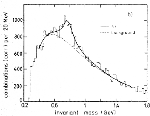
Figure 4.2: Typical invariant mass spectrum of pion pairs produced in semi-inclusive DIS [29]. The $\rho$ peak is visible.

The situation is different for proton-pion production, where on top of the smooth $s$-wave continuum the sharp spin-half $\Lambda(1115)$ resonance appears. Since the $\Lambda$ undergoes a parity-violating weak decay the formalism we will develop in this chapter will prove to be inadequate. Moreover, the resonance is so sharp that it is more appropriate and easier to study it in the framework of polarized single hadron production. For these reasons, although polarized $\Lambda$ production represents a very nice way to observe the transversity distribution, we will not touch this subject, for which it is possible to consult a vast literature [84, 28, 18, 19, 20, 22, 13, 16, 17, 14, 86].

4.1.1 Kinematics

We assume to detect two hadrons with masses $M_{1}$ and $M_{2}$ and momenta $P_{1}$ and $P_{2}$. We denote the center-of-mass momentum as $P_{h}$ and the total invariant mass of the system as $M_{h}$. We maintain the parametrization of the vectors $P$, $P_{h}$ and $q$ as given in Eqs. (3.3) and Eqs. (3.10), but we introduce also the semi-difference of the two hadrons’ momenta, $R$. We parametrize the new momenta according to

$$R^{\mu} =\biggl{[}\frac{\zeta}{2}\,P_{h}^{-},\;\frac{\left(M_{1}^{2}-M_{2}^{2}\right)-\frac{\zeta}{2}\,M_{h}^{2}}{2P_{h}^{-}},\;\bm{R}_{T}\biggr{]},$$ (4.1a)

$$P_{1}^{\mspace{2.0mu}\mu}=\frac{P_{h}^{\mu}}{2}+R^{\mu} =\biggl{[}\frac{(1+\zeta)}{2}\,P_{h}^{-},\;\frac{\left(M_{1}^{2}-M_{2}^{2}\right)+\frac{(1-\zeta)}{2}\,M_{h}^{2}}{2P_{h}^{-}},\;\bm{R}_{T}\biggr{]},$$ (4.1b)

$$P_{2}^{\mspace{2.0mu}\mu}=\frac{P_{h}^{\mu}}{2}-R^{\mu} =\biggl{[}\frac{(1-\zeta)}{2}\,P_{h}^{-},\;\frac{\left(M_{1}^{2}-M_{2}^{2}\right)+\frac{(1+\zeta)}{2}\,M_{h}^{2}}{2P_{h}^{-}},\;-\bm{R}_{T}\biggr{]}.$$ (4.1c)

The total invariant mass squared, $M_{h}^{2}$, has to be small compared to $Q^{2}$. For later convenience, we compute the scalar quantities

$$R^{2} =\frac{\left(M_{1}^{2}+M_{2}^{2}\right)}{2}-\frac{M_{h}^{2}}{4},$$ (4.2a)

$$\bm{R}_{T}^{2} =\frac{1}{2}\,\biggl{[}\frac{(1-\zeta)(1+\zeta)}{2}M_{h}^{2}-(1-\zeta)M_{1}^{2}-(1+\zeta)M_{2}^{2}\biggr{]},$$ (4.2b)

$$P_{h}\cdot R =\frac{\left(M_{1}^{2}-M_{2}^{2}\right)}{2},$$ (4.2c)

$$P_{h}\cdot k =\frac{M_{h}^{2}}{2z}+z\,\frac{k^{2}+\lvert\bm{k}_{T}\rvert^{2}}{2},$$ (4.2d)

$$k\cdot R =\frac{\left(M_{1}^{2}-M_{2}^{2}\right)-\frac{\zeta}{2}\,M_{h}^{2}}{2z}+z\,\zeta\;\frac{k^{2}+\lvert\bm{k}_{T}\rvert^{2}}{4}-\bm{k}_{T}\cdot\bm{R}_{T}.$$ (4.2e)

4.1.2 The hadronic tensor

For a process with two outgoing hadrons we can define the cross section

$$\frac{2E_{1}\,2E_{2}\operatorname{{\rm\,d}}^{9}\!\sigma}{\operatorname{{\rm\,d}}^{3}\!\bm{P}_{1}\operatorname{{\rm\,d}}^{3}\!\bm{P}_{2}\operatorname{{\rm\,d}}x_{B}\operatorname{{\rm\,d}}y\operatorname{{\rm\,d}}\phi_{S}}=\frac{\alpha^{2}}{2sx_{B}Q^{2}}\,L_{\mu\nu}(l,l^{\prime},\lambda_{e})\,2MW^{\mu\nu}(q,P,S,P_{1},P_{2}),$$ (4.3)

which can be rewritten in terms of the different variables as

$$\frac{\operatorname{{\rm\,d}}^{9}\!\sigma}{\operatorname{{\rm\,d}}\zeta\operatorname{{\rm\,d}}M_{h}^{2}\operatorname{{\rm\,d}}\phi_{R}\operatorname{{\rm\,d}}z_{h}\operatorname{{\rm\,d}}^{2}\!\bm{P}_{h\perp}\operatorname{{\rm\,d}}x_{B}\operatorname{{\rm\,d}}y\operatorname{{\rm\,d}}\phi_{S}}=\frac{\alpha^{2}}{32\,z_{h}sx_{B}Q^{2}}\,L_{\mu\nu}(l,l^{\prime},\lambda_{e})\,2MW^{\mu\nu}(q,P,S,P_{1},P_{2}).$$ (4.4)

The angle $\phi_{R}$ is the azimuthal angle of the vector $\bm{R}_{T}$ with respect to the lepton plane, measured in a plane perpendicular to the direction of the outgoing hadron. Neglecting $1/Q$ corrections, it can be identified with the azimuthal angle measured in a plane perpendicular to the virtual photon direction or to the lepton beam. Notice the extra factor 8 in the denominator compared to the one-particle inclusive case. To obtain the previous formula, we made use of the steps

$$\begin{split}\frac{\operatorname{{\rm\,d}}^{3}\!\bm{P}_{1}\operatorname{{\rm\,d}}^{3}\!\bm{P}_{2}}{2E_{1}\,2E_{2}}&=\frac{\operatorname{{\rm\,d}}^{3}\!\bm{P}_{h}\operatorname{{\rm\,d}}^{3}\!\bm{R}}{E_{h}^{2}\left(1-4E_{R}^{2}/E_{h}^{2}\right)}\approx\frac{\operatorname{{\rm\,d}}z_{h}\operatorname{{\rm\,d}}^{2}\!\bm{P}_{h\perp}\operatorname{{\rm\,d}}\zeta\operatorname{{\rm\,d}}^{2}\!\bm{R}_{T}}{z^{2}(1-\zeta^{2})}\\ &=\frac{\operatorname{{\rm\,d}}z_{h}\operatorname{{\rm\,d}}^{2}\!\bm{P}_{h\perp}\operatorname{{\rm\,d}}\zeta\operatorname{{\rm\,d}}^{2}\!\bm{R}_{T}}{2z_{h}(1-\zeta^{2})}=\frac{\operatorname{{\rm\,d}}z_{h}\operatorname{{\rm\,d}}^{2}\!\bm{P}_{h}\operatorname{{\rm\,d}}\zeta\operatorname{{\rm\,d}}M_{h}^{2}\operatorname{{\rm\,d}}\phi_{R}}{16z_{h}}\,.\end{split}$$ (4.5)

The hadronic tensor for two-particle inclusive scattering is defined as

$$\begin{split}2MW^{\mu\nu}(q,P,S,P_{1},P_{2})&=\frac{1}{(2\pi)^{7}}\sum_{\cal X^{\prime\prime}}\int\frac{\operatorname{{\rm\,d}}^{3}\!\bm{P}_{\cal X^{\prime\prime}}}{(2\pi)^{3}\,2P_{X^{\prime\prime}}^{0}}\;\\ &\quad\times(2\pi)^{4}\,\delta^{(4)}\bigl{(}q+P-P_{\cal X^{\prime\prime}}-P_{1}-P_{2}\bigr{)}\,H^{\mu\nu}(P,S,P_{\cal X^{\prime\prime}},P_{1},P_{2}),\end{split}$$ (4.6)

$$H^{\mu\nu}(P,S,P_{\cal X^{\prime\prime}},P_{1},P_{2}) =\bigl{\langle}{P,S}\mspace{2.0mu}\raisebox{-3.0pt}{\rule{0.7pt}{12.0pt}}\;J^{\mu}(0)\;\raisebox{-3.0pt}{\rule{0.7pt}{12.0pt}}\,{P_{1},P_{2},{\cal X^{\prime\prime}}}\bigr{\rangle}\bigl{\langle}{P_{1},P_{2},{\cal X^{\prime\prime}}}\mspace{2.0mu}\raisebox{-3.0pt}{\rule{0.7pt}{12.0pt}}\;J^{\nu}(0)\;\raisebox{-3.0pt}{\rule{0.7pt}{12.0pt}}\,{P,S}\bigr{\rangle}.$$ (4.7)

With this definition, it is possible to recover the hadronic tensor for one-particle inclusive scattering by integration over the second hadron

$$\begin{split}\@ADDCLASS{ltx_eqn_lefteqn}$\displaystyle\sum_{h_{2}}\int\frac{\operatorname{{\rm\,d}}^{3}\!\bm{P}_{2}}{2P_{2}^{0}}\;2MW^{\mu\nu}(q,P,S,P_{1},P_{2})$\mbox{}\hfil\\ &=\sum_{h_{2}}\int\frac{\operatorname{{\rm\,d}}^{3}\!\bm{P}_{2}}{(2\pi)^{3}\,2P_{2}^{0}}\sum_{\cal X^{\prime\prime}}\int\frac{\operatorname{{\rm\,d}}^{3}\!\bm{P}_{\cal X^{\prime\prime}}}{(2\pi)^{3}\,2P_{X^{\prime\prime}}^{0}}\;\delta^{(4)}\bigl{(}q+P-P_{\cal X^{\prime\prime}}-P_{2}-P_{1}\bigr{)}\,H^{\mu\nu}(P,S,P_{\cal X^{\prime\prime}},P_{1},P_{2})\\ &=\sum_{\cal X^{\prime}}\int\frac{\operatorname{{\rm\,d}}^{3}\!\bm{P}_{\cal X^{\prime}}}{(2\pi)^{3}\,2P_{X^{\prime}}^{0}}\;\delta^{(4)}\bigl{(}q+P-P_{\cal X^{\prime}}-P_{1}\bigr{)}\,\int\frac{\operatorname{{\rm\,d}}^{3}\!\bm{P}_{2}}{(2\pi)^{3}\,2P_{2}^{0}}\,H^{\mu\nu}(P,S,P_{\cal X^{\prime}}-P_{2},P_{1},P_{2})\\ &=\sum_{\cal X^{\prime}}\int\frac{\operatorname{{\rm\,d}}^{3}\!\bm{P}_{\cal X^{\prime}}}{(2\pi)^{3}\,2P_{\cal X^{\prime}}^{0}}\;\delta^{(4)}\bigl{(}q+P-P_{\cal X^{\prime}}-P_{1}\bigr{)}\,H^{\mu\nu}(P,S,P_{\cal X^{\prime}},P_{1})\equiv 2MW^{\mu\nu}(q,P,S,P_{1})\end{split}$$ (4.8)

where the state $\cal X^{\prime}$ represents the sum of the states $\cal X^{\prime\prime}$ plus all possible states of the second hadron, and $P_{\cal X^{\prime}}=P_{\cal X^{\prime\prime}}+P_{2}$.

In analogy to what we presented in Sec. 3.1.2, at leading order in $1/Q$ the hadronic tensor can be expressed in terms of correlation functions as

$$2MW^{\mu\nu}(q,P,S,P_{1},P_{2})=32z_{h}\,\,{\cal I}\Bigl{[}\operatorname{Tr}{\left(\Phi(x_{B},\bm{p}_{T},S)\;\gamma^{\mspace{2.0mu}\mu}\;\Delta(z_{h},\bm{k}_{T},\zeta,M_{h}^{2},\phi_{R})\;\gamma^{\nu}\right)}\Bigr{]},$$ (4.9)

where the fragmentation correlation function has been generalized to include also the dependence on the vector $R$

$$\Delta(z,\zeta,M_{h}^{2},\phi_{R},\bm{k}_{T})\equiv\frac{1}{32z}\int\operatorname{{\rm\,d}}k^{+}\Delta(k,P_{h},R)\Bigr{|}_{k^{-}=P_{h}^{-}/z}.$$ (4.10)

The fully differential cross section might be a little bit too complex for experimental measurements. To simplify the situation, we can perform the integration over the transverse part of the center-of-mass momentum, $\bm{P}_{h\perp}$. The integrated cross section is

$$\frac{\operatorname{{\rm\,d}}^{7}\!\sigma}{\operatorname{{\rm\,d}}\zeta\operatorname{{\rm\,d}}M_{h}^{2}\operatorname{{\rm\,d}}\phi_{R}\operatorname{{\rm\,d}}z_{h}\operatorname{{\rm\,d}}x_{B}\operatorname{{\rm\,d}}y\operatorname{{\rm\,d}}\phi_{S}}=\frac{\alpha^{2}}{32z_{h}sx_{B}Q^{2}}\,L_{\mu\nu}(l,l^{\prime},\lambda_{e})\,2MW^{\mu\nu}(q,P,S,P_{1},P_{2}),$$ (4.11)

where

$$2MW^{\mu\nu}(q,P,S,P_{1},P_{2}) =32z_{h}\,\operatorname{Tr}{\left[\Phi(x_{B},S)\;\gamma^{\mspace{2.0mu}\mu}\;\Delta(z_{h},\zeta,M_{h}^{2},\phi_{R})\;\gamma^{\nu}\right]}.$$ (4.12a)

$$\Delta(z,\zeta,M_{h}^{2},\phi_{R}) \equiv\frac{z}{32}\int\operatorname{{\rm\,d}}k^{+}\operatorname{{\rm\,d}}^{2}\!\bm{k}_{T}\,\Delta(k,P_{h},R)\Bigr{|}_{k^{-}=P_{h}^{-}/z}.$$ (4.12b)

To identify the leading twist part of the hadronic tensor and write down the cross section, we can trivially repeat the steps described in Sec. 3.1.3.

4.2 The correlation function $\Delta$

The most general expansion of the quark-quark correlation matrix $\Delta$, respecting Hermiticity and parity invariance, is [44]

$$\begin{split}\Delta(k,P_{h},R)&=M_{h}\,C_{1}\,{\bm{1}}+C_{2}\,\makebox[0.0pt][l]{\hskip 1.2pt$\sslash$}{P}_{h}+C_{3}\,\makebox[0.0pt][l]{\hskip 1.2pt$\sslash$}{R}+C_{4}\,\makebox[0.0pt][l]{$\sslash$}{k}\\ &\quad+\frac{C_{5}}{M_{h}}\,\sigma_{\mu\nu}P_{h}^{\mspace{2.0mu}\mu}k^{\nu}+\frac{C_{6}}{M_{h}}\,\sigma_{\mu\nu}R^{\mu}k^{\nu}+\frac{C_{7}}{M_{h}}\,\sigma_{\mu\nu}P_{h}^{\mspace{2.0mu}\mu}R^{\nu}+\frac{C_{8}}{M_{h}^{2}}\,\gamma_{5}\epsilon^{\mspace{2.0mu}\mu\nu\rho\sigma}\gamma_{\mu}P_{h\nu}R_{\rho}k_{\sigma}.\end{split}$$ (4.13)

The amplitudes $C_{i}$ are dimensionless real scalar functions $C_{i}=C_{i}(k\cdot P_{h},k^{2},R^{2},k\cdot R)$. The last four terms are T-odd.

We are going to consider first the case when no hadron transverse momentum, $\bm{P}_{h\perp}$, is detected and postpone the complete case to the second part of the chapter. We insert the general decomposition of Eq. (4.13) into Eq. (3.17c) and extract the leading-twist projection

$${\cal P}_{-}\,\Delta(z,\zeta,M_{h}^{2},\phi_{R})\,\gamma^{-}=\frac{1}{8\pi}\left(D_{1}(z,\zeta,M_{h}^{2})+i\,H_{1}^{\sphericalangle}(z,\zeta,M_{h}^{2})\,\frac{\makebox[0.0pt][l]{\hskip 1.2pt$\sslash$}{R}_{T}}{M_{h}}\right){\cal P}_{-}\,,$$ (4.14)

The prefactor has been chosen to have a better connection with one-hadron results, i.e. integrated over $\zeta$, $M_{h}^{2}$ and $\phi_{R}$. We introduced the two-hadron parton fragmentation functions

$$D_{1}(z,\zeta,M_{h}^{2}) =\frac{z}{2}\int\operatorname{{\rm\,d}}^{2}\!\bm{k}_{T}\operatorname{{\rm\,d}}k^{2}\operatorname{{\rm\,d}}(2k\cdot P_{h})\;\delta\left(\bm{k}_{T}^{2}+\frac{M_{h}^{2}}{z^{2}}+k^{2}-\frac{2k\cdot P_{h}}{z}\right)\;\left[C_{2}+\frac{\zeta}{2}C_{3}+\frac{1}{z}C_{4}\right],$$ (4.15a)

$$H_{1}^{\sphericalangle}(z,\zeta,M_{h}^{2}) =\frac{z}{2}\int\operatorname{{\rm\,d}}^{2}\!\bm{k}_{T}\operatorname{{\rm\,d}}k^{2}\operatorname{{\rm\,d}}(2k\cdot P_{h})\;\delta\left(\bm{k}_{T}^{2}+\frac{M_{h}^{2}}{z^{2}}+k^{2}-\frac{2k\cdot P_{h}}{z}\right)\;\left[-C_{7}+\frac{1}{z}C_{6}\right].$$ (4.15b)

The fragmentation function $H_{1}^{\sphericalangle}$ is chiral-odd and T-odd. Like the Collins function, it can be used as a partner for the transversity distribution, as we will see in the next section. Notice that this function does not require the presence of partonic transverse momentum. Because of this, its evolution equations could be simpler than the ones of the Collins function. Since this function has the same operator structure as the transversity, it has been suggested that it could have the same evolution equations [55, 160, 56]. However, the situation could be complicated by the presence of the dependence on the variables $\zeta$ and $M_{h}^{2}$, which are not present in single particle functions [161].

4.2.1 Correlation function in helicity formalism

Once again, expressing the Dirac matrices of Eq. (4.14) in the chiral or Weyl representation, we obtain

$$\Bigl{(}{\cal P}_{-}\,\Delta(z,\zeta,M_{h}^{2},\phi_{R})\,\gamma^{-}\Bigr{)}_{kl}=\frac{1}{8\pi}\begin{pmatrix}0&0&0&0\\ 0&D_{1}(z,\zeta,M_{h}^{2})&{\rm i}{\rm e}^{{\rm i}\phi_{R}}\,\dfrac{\left\lvert\bm{R}_{T}\right\rvert}{M_{h}}\,H_{1}^{\sphericalangle}(z,\zeta,M_{h}^{2})&0\\ 0&-{\rm i}{\rm e}^{-{\rm i}\phi_{R}}\,\dfrac{\left\lvert\bm{R}_{T}\right\rvert}{M_{h}}\,H_{1}^{\sphericalangle}(z,\zeta,M_{h}^{2})&D_{1}(z,\zeta,M_{h}^{2})&0\\ 0&0&0&0\end{pmatrix}.$$ (4.16)

As already observed before, we can restrict ourselves to the subspace of good quark fields and adopt the chirality basis, and rewrite the correlation function as

$$D(z,\zeta,M_{h}^{2},\phi_{R})_{\chi^{\prime}_{2}\chi^{\phantom{{}^{\prime}}}_{2}}=\frac{1}{8\pi}\begin{pmatrix}D_{1}(z,\zeta,M_{h}^{2})&{\rm i}{\rm e}^{{\rm i}\phi_{R}}\dfrac{\left\lvert\bm{R}_{T}\right\rvert}{M_{h}}H_{1}^{\sphericalangle}(z,\zeta,M_{h}^{2})\\ -{\rm i}{\rm e}^{-{\rm i}\phi_{R}}\dfrac{\left\lvert\bm{R}_{T}\right\rvert}{M_{h}}H_{1}^{\sphericalangle}(z,\zeta,M_{h}^{2})&D_{1}(z,\zeta,M_{h}^{2})\end{pmatrix}.$$ (4.17)

From the positivity of the previous matrix, we can derive bounds for the two-hadron fragmentation functions defined above:

$$D_{1}(z,\zeta,M_{h}^{2}) \geq 0,$$ (4.18a)

$$\frac{\left\lvert\bm{R}_{T}\right\rvert}{M_{h}}\left\lvert H_{1}^{\sphericalangle}(z,\zeta,M_{h}^{2})\right\rvert \leq D_{1}(z,\zeta,M_{h}^{2}).$$ (4.18b)

4.3 Cross section and asymmetries

In Fig. 4.3, we give a pictorial description of the vectors and angles involved in one-particle inclusive deep inelastic scattering.

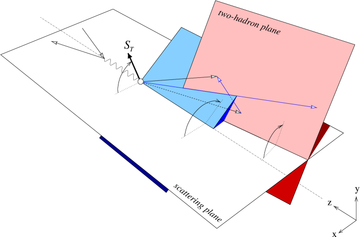
Figure 4.3: Description of the vectors and angles involved in two-particle inclusive deep inelastic scattering.

The differential cross section integrated over the center-of-mass transverse momentum reads

$$\frac{\operatorname{{\rm\,d}}^{7}\!\sigma}{\operatorname{{\rm\,d}}\zeta\operatorname{{\rm\,d}}M_{h}^{2}\operatorname{{\rm\,d}}\phi_{R}\operatorname{{\rm\,d}}z_{h}\operatorname{{\rm\,d}}x_{B}\operatorname{{\rm\,d}}y\operatorname{{\rm\,d}}\phi_{S}}=\sum_{q}\,\rho(S)_{\Lambda^{\phantom{{}^{\prime}}}_{1}\Lambda_{1}^{\prime}}\;F(x_{B})_{\chi^{\phantom{{}^{\prime}}}_{1}\chi^{\prime}_{1}}^{\Lambda_{1}^{\prime}\Lambda^{\phantom{{}^{\prime}}}_{1}}\Bigl{(}\frac{\operatorname{{\rm\,d}}\sigma^{eq}}{\operatorname{{\rm\,d}}y}\Bigr{)}^{\chi^{\phantom{{}^{\prime}}}_{1}\chi^{\prime}_{1};\,\chi^{\phantom{{}^{\prime}}}_{2}\chi^{\prime}_{2}}\,D(z_{h},\zeta,M_{h}^{2},\phi_{R})_{\chi^{\prime}_{2}\chi^{\phantom{{}^{\prime}}}_{2}}.$$ (4.19)

Inserting into the previous equation the formulae obtained for the distribution correlation matrix, Eq. (2.48), the elementary cross section, Eq. (3.21), and the two-hadron fragmentation matrix, Eq. (4.17), we obtain the following result

$$\frac{\operatorname{{\rm\,d}}^{7}\!\sigma}{\operatorname{{\rm\,d}}\zeta\operatorname{{\rm\,d}}M_{h}^{2}\operatorname{{\rm\,d}}\phi_{R}\operatorname{{\rm\,d}}z_{h}\operatorname{{\rm\,d}}x_{B}\operatorname{{\rm\,d}}y\operatorname{{\rm\,d}}\phi_{S}}=\frac{2\alpha^{2}}{4\pi sx_{B}y^{2}}\,\sum_{q}e_{q}^{2}\,\Biggl{[}A(y)\,f_{1}^{q}(x_{B})D_{1}^{q}(z,\zeta,M_{h}^{2})\\ +\lambda_{e}\,S_{L}\,C(y)\,g_{1}^{q}(x_{B})D_{1}^{q}(z,\zeta,M_{h}^{2})+B(y)\,|\bm{S}_{\perp}|\,\frac{|\bm{R}_{T}|}{M_{h}}\,\sin(\phi_{R}+\phi_{S})\,h_{1}^{q}(x_{B})H_{1}^{\sphericalangle q}(z,\zeta,M_{h}^{2})\Biggr{]}.$$ (4.20)

4.3.1 Transversity measurements

To access transversity in two-particle inclusive deep inelastic scattering it is required to measure the azimuthal single transverse spin asymmetry [150]

$$\begin{split}\left\langle\sin(\phi_{R}+\phi_{S})\right\rangle_{UT}(x_{B},y,z_{h})&\equiv\frac{\int\operatorname{{\rm\,d}}\phi_{S}\,\operatorname{{\rm\,d}}\phi_{R}\,\operatorname{{\rm\,d}}\zeta\,\operatorname{{\rm\,d}}M_{h}^{2}\,\sin(\phi_{R}+\phi_{S})\,\operatorname{{\rm\,d}}^{7}\!\sigma_{UT}}{\int\operatorname{{\rm\,d}}\phi_{S}\,\operatorname{{\rm\,d}}\phi_{R}\,\operatorname{{\rm\,d}}\zeta\,\operatorname{{\rm\,d}}M_{h}^{2}\,\operatorname{{\rm\,d}}^{7}\!\sigma_{UU}}\\ &=|\bm{S}_{T}|\frac{(1/x_{B}y^{2})\,B(y)\,\sum_{q}e_{q}^{2}\,h_{1}^{q}(x_{B})\,\int\operatorname{{\rm\,d}}\zeta\,\operatorname{{\rm\,d}}M_{h}^{2}\,\dfrac{|\bm{R}_{T}|}{2M_{h}}\,H_{1}^{\sphericalangle q}(z_{h},\zeta,M_{h}^{2})}{(1/x_{B}y^{2})\,A(y)\,\sum_{q}e_{q}^{2}\,f_{1}^{q}(x_{B})\,\int\operatorname{{\rm\,d}}\zeta\,\operatorname{{\rm\,d}}M_{h}^{2}\,D_{1}^{q}(z_{h},\zeta,M_{h}^{2})}\;.\end{split}$$ (4.21)

The most valuable characteristic of this asymmetry is that it does not require the measurement of the center of mass transverse momentum, so that the complications connected to the inclusion of partonic transverse momenta can be avoided. Apart from the usual variables $x_{B}$, $y$, $z_{h}$, the only other variable to be measured is the angle $\phi_{R}+\phi_{S}$. In case the transverse spin direction is used as a reference axis, instead of the lepton scattering plane, then the angle to be measured is $\phi_{R}^{S}-2\phi_{l}^{S}$.

4.4 Partial wave expansion

Up to now, we did not make any study of the inner structure of the two-hadron fragmentation functions. It is useful to expand them in partial waves, because if we restrict ourselves to systems with low invariant masses, the dominant contributions come only from the lowest harmonics, i.e. $s$ and $p$ waves.

4.4.1 Center-of-mass parameters

The partial-wave expansion can be performed only in the frame of reference of the center of mass of the hadron pair. As a first step, we need to express all vectors in this frame, i.e. 

$$P_{h}^{\mspace{2.0mu}\mu} \overset{\rm cm}{=}\Biggl{[}\frac{M_{h}}{\sqrt{2}},\;\frac{M_{h}}{\sqrt{2}},\;0,\;0\Biggr{]},$$ (4.22a)

$$\begin{split}R^{\mu}&\overset{\rm cm}{=}\Biggl{[}\frac{\sqrt{M_{1}^{2}+\lvert\bm{R}\rvert^{2}}-\sqrt{M_{2}^{2}+\lvert\bm{R}\rvert^{2}}-2\lvert\bm{R}\rvert\cos{\theta}}{2\sqrt{2}},\;\\ &\qquad\frac{\sqrt{M_{1}^{2}+\lvert\bm{R}\rvert^{2}}-\sqrt{M_{2}^{2}+\lvert\bm{R}\rvert^{2}}+2\lvert\bm{R}\rvert\cos{\theta}}{2\sqrt{2}},\;\lvert\bm{R}\rvert\sin{\theta}\cos{\phi_{R}},\;\lvert\bm{R}\rvert\sin{\theta}\sin{\phi_{R}}\Biggr{]},\end{split}$$ (4.22b)

$$P_{1}^{\mspace{2.0mu}\mu} \overset{\rm cm}{=}\Biggl{[}\frac{\sqrt{M_{1}^{2}+\lvert\bm{R}\rvert^{2}}-\lvert\bm{R}\rvert\cos{\theta}}{\sqrt{2}},\;\frac{\sqrt{M_{1}^{2}+\lvert\bm{R}\rvert^{2}}+\lvert\bm{R}\rvert\cos{\theta}}{\sqrt{2}},\;\lvert\bm{R}\rvert\sin{\theta}\cos{\phi_{R}},\;\lvert\bm{R}\rvert\sin{\theta}\sin{\phi_{R}}\Biggr{]},$$ (4.22c)

$$P_{2}^{\mspace{2.0mu}\mu} \overset{\rm cm}{=}\Biggl{[}\frac{\sqrt{M_{2}^{2}+\lvert\bm{R}\rvert^{2}}-\lvert\bm{R}\rvert\cos{\theta}}{\sqrt{2}},\;\frac{\sqrt{M_{2}^{2}+\lvert\bm{R}\rvert^{2}}+\lvert\bm{R}\rvert\cos{\theta}}{\sqrt{2}},\;-\lvert\bm{R}\rvert\sin{\theta}\cos{\phi_{R}},\;-\lvert\bm{R}\rvert\sin{\theta}\sin{\phi_{R}}\Biggr{]},$$ (4.22d)

where

$$\lvert\bm{R}\rvert=\frac{1}{2}\sqrt{M_{h}^{2}-2\left(M_{1}^{2}+M_{2}^{2}\right)+\left(M_{1}^{2}-M_{2}^{2}\right)^{2}\bigg{/}M_{h}^{2}}.$$ (4.23)

The polar angle $\theta$ is illustrated in Fig. 4.4.

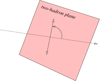
Figure 4.4: Description of the polar angle $\theta$, in the center-of-mass frame of the hadron couple.

The variable $\zeta$ is connected to the center-of-mass variable $\cos{\theta}$ in the following way:

$$\zeta\equiv\frac{2R^{-}}{P_{h}^{-}}\overset{\rm cm}{=}\frac{1}{M_{h}}\left(\sqrt{M_{1}^{2}+\lvert\bm{R}\rvert^{2}}-\sqrt{M_{2}^{2}+\lvert\bm{R}\rvert^{2}}-2\lvert\bm{R}\rvert\cos{\theta}\right).$$ (4.24)

If $M_{1}=M_{2}$, notice that $R$ is purely spacelike and

$$\lvert\bm{R}\rvert =-|R|=\frac{1}{2}\sqrt{M_{h}^{2}-4M_{1}^{2}}, \zeta =-\frac{1}{M_{h}}\sqrt{M_{h}^{2}-4M_{1}^{2}}\,\cos{\theta}.$$ (4.25)

4.4.2 The correlation function $\Delta$ with partial wave-expansion

To perform the partial-wave expansion of the fragmentation functions, let us first express the correlation function $\Delta$ in terms of center-of-mass parameters

$${\cal P}_{-}\,\Delta(z,\zeta(\cos\theta),M_{h}^{2},\phi_{R})\,\gamma^{-}=\frac{1}{8\pi}\left(D_{1}\bigl{(}z,\zeta(\cos{\theta}),M_{h}^{2}\bigr{)}+{\rm i}H_{1}^{\sphericalangle}\bigl{(}z,\zeta(\cos{\theta}),M_{h}^{2}\bigr{)}\,\sin{\theta}\,\frac{\lvert\bm{R}\rvert}{M_{h}}\,\makebox[0.0pt][l]{\hskip 1.0pt$\sslash$}{n}_{\phi_{R}}\right){\cal P}_{-}\,,$$ (4.26)

where $n_{\phi_{R}}^{\mu}=\bigl{[}0,\;0,\;\cos{\phi_{R}},\;\sin{\phi_{R}}\bigr{]}$. In general, we can expand the fragmentation functions on the basis of the Legendre polynomials in the following way

$$D_{1}\bigl{(}z,\zeta(\cos{\theta}),M_{h}^{2}\bigr{)}=\sum_{n}D_{1n}\bigl{(}z,M_{h}^{2}\bigr{)}\,P_{n}(\cos{\theta})$$ (4.27)

with

$$D_{1n}\bigl{(}z,M_{h}^{2}\bigr{)}=\int_{-1}^{1}\operatorname{{\rm\,d}}\cos{\theta}\;P_{n}(\cos{\theta})\,D_{1}\bigl{(}z,\zeta(\cos{\theta}),M_{h}^{2}\bigr{)}.$$ (4.28)

Considering only two-hadron systems with a low invariant mass, we assume we can truncate the expansion in order to include only $s$-wave and $p$-wave contributions to the correlation function. The connection between the correlation function $\Delta$ in terms of the variable $\zeta$ and in terms of the variable $\cos\theta$ is

$$\Delta(z,\cos\theta,M_{h}^{2},\phi_{R})=\frac{2\lvert\bm{R}\rvert}{M_{h}}\,\Delta(z,\zeta,M_{h}^{2},\phi_{R}),$$ (4.29)

to take into account the fact that $\operatorname{{\rm\,d}}\zeta=2\lvert\bm{R}\rvert/M_{h}\operatorname{{\rm\,d}}\cos\theta$. Then we can write the partial-wave expanded correlation function as

$$\begin{split}{\cal P}_{-}\,\Delta(z,\cos\theta,M_{h}^{2},\phi_{R})\,\gamma^{-}&\approx\frac{1}{8\pi}\Biggl{[}D_{1,UU}\bigl{(}z,M_{h}^{2}\bigr{)}+D_{1,UL}^{sp}\bigl{(}z,M_{h}^{2}\bigr{)}\,\cos{\theta}+D_{1,LL}^{pp}\bigl{(}z,M_{h}^{2}\bigr{)}\,\frac{1}{4}\left(3\cos^{2}{\theta}-1\right)\\ &\quad+{\rm i}\left(H_{1,UT}^{\sphericalangle\,sp}\bigl{(}z,M_{h}^{2}\bigr{)}+H_{1,LT}^{\sphericalangle\,pp}\bigl{(}z,M_{h}^{2}\bigr{)}\cos{\theta}\right)\,\sin{\theta}\,\frac{\lvert\bm{R}\rvert}{M_{h}}\,\makebox[0.0pt][l]{\hskip 1.0pt$\sslash$}{n}_{\phi_{R}}\Biggr{]}\,{\cal P}_{-}\,,\end{split}$$ (4.30)

The correlation function can be consequently written in matrix form as

$$D(z,\cos\theta,M_{h}^{2},\phi_{R})_{\chi^{\prime}_{2}\chi^{\phantom{{}^{\prime}}}_{2}}\approx\\ \frac{1}{8\pi}\begin{pmatrix}D_{1,UU}+D_{1,UL}^{sp}\cos{\theta}+D_{1,LL}^{pp}\,\frac{1}{4}\left(3\cos^{2}{\theta}-1\right)&+{\rm i}\left(H_{1,UT}^{\sphericalangle\,sp}+H_{1,LT}^{\sphericalangle\,pp}\cos{\theta}\right)\sin{\theta}\,\dfrac{\lvert\bm{R}\rvert}{M_{h}}\,{\rm e}^{{\rm i}\phi_{R}}\\ -{\rm i}\left(H_{1,UT}^{\sphericalangle\,sp}+H_{1,LT}^{\sphericalangle\,pp}\cos{\theta}\right)\sin{\theta}\,\dfrac{\lvert\bm{R}\rvert}{M_{h}}\,{\rm e}^{-{\rm i}\phi_{R}}&D_{1,UU}+D_{1,UL}^{sp}\cos{\theta}+D_{1,LL}^{pp}\,\frac{1}{4}\left(3\cos^{2}{\theta}-1\right)\end{pmatrix}.$$ (4.31)

Here, it is not yet clear what are the motivations to assign such names to the functions. It will become clear after we distinguish the $s$- and $p$-wave contributions in the rest of the section and also after we study spin-one fragmentation functions in Chap. 5.

The information encoded in the correlation function can be expressed in a different way. Depending on the angular momentum of the system, the angular distribution of the two hadrons is characterized by a specific bilinear combination of spherical harmonics. If the angular momentum can be only 0 or 1, as in the case of our truncated partial wave expansion, the angular distribution of the two hadrons can be fully described by the decay matrix

$${\cal D}(\theta,\phi_{R})_{jm,j^{\prime}m^{\prime}}=Y_{j}^{m}\,Y_{j^{\prime}}^{m^{\prime}\,\ast}=\\ \frac{1}{4\pi}\left(\begin{array}[]{c|ccc}1&-\sqrt{{\frac{3}{2}}}\sin{\theta}\,{\rm e}^{{\rm i}\phi_{R}}&\sqrt{3}\cos{\theta}&\sqrt{{\frac{3}{2}}}\sin{\theta}\,{\rm e}^{-{\rm i}\phi_{R}}\\[3.0pt] \hline\cr-\sqrt{{\frac{3}{2}}}\sin{\theta}\,{\rm e}^{-{\rm i}\phi_{R}}&\frac{3}{2}\sin^{2}{\theta}&-\frac{3}{\sqrt{2}}\cos{\theta}\sin{\theta}\,{\rm e}^{-{\rm i}\phi_{R}}&-\frac{3}{2}\sin^{2}{\theta}\,{\rm e}^{-2{\rm i}\phi_{R}}\\ \sqrt{3}\cos{\theta}&-\frac{3}{\sqrt{2}}\cos{\theta}\sin{\theta}\,{\rm e}^{{\rm i}\phi_{R}}&3\cos^{2}{\theta}&\frac{3}{\sqrt{2}}\cos{\theta}\sin{\theta}\,{\rm e}^{-{\rm i}\phi_{R}}\\ \sqrt{{\frac{3}{2}}}\sin{\theta}\,{\rm e}^{{\rm i}\phi_{R}}&-\frac{3}{2}\sin^{2}{\theta}\,{\rm e}^{2{\rm i}\phi_{R}}&\frac{3}{\sqrt{2}}\cos{\theta}\sin{\theta}\,{\rm e}^{{\rm i}\phi_{R}}&\frac{3}{2}\sin^{2}{\theta}\end{array}\right).$$ (4.32)

The angular momentum indices, $j$ and $j^{\prime}$, run only from 0 to 1. For convenience, we split the matrix into blocks: the upper-left block ($j=j^{\prime}=0$) refers to the pure $s$-wave component, the lower-right block ($j=j^{\prime}=1$) describes the $p$-wave component, and it is subdivided according to the value of $m,m^{\prime}=+1,0,-1$, Finally, the off-diagonal blocks describe the $sp$ interference.

The original correlation function can now be expressed as the trace of the decay matrix and a fragmentation matrix in the quark chirality space $\otimes$ the hadronic system angular momentum space

$$D(z,\cos\theta,M_{h}^{2},\phi_{R})_{\chi^{\prime}_{2}\chi^{\phantom{{}^{\prime}}}_{2}}=D(z,M_{h}^{2})_{\chi^{\prime}_{2}\chi^{\phantom{{}^{\prime}}}_{2}}^{j^{\prime}m^{\prime},jm}{\cal D}(\theta,\phi_{R})_{jm,j^{\prime}m^{\prime}}.$$ (4.33)

The solution for the fragmentation matrix is the $8\times 8$ matrix

$$D(z,M_{h}^{2})_{\chi^{\prime}_{2}\chi^{\phantom{{}^{\prime}}}_{2}}^{j^{\prime}m^{\prime},jm}=\frac{1}{8}\,\begin{pmatrix}A_{j^{\prime}m^{\prime},jm}&B_{j^{\prime}m^{\prime},jm}\\ B_{j^{\prime}m^{\prime},jm}^{\dagger}&A_{j^{\prime}m^{\prime},jm}\end{pmatrix},$$ (4.34)

where the inner blocks, spanning the hadronic angular momentum space, read explicitly

$$A_{j^{\prime}m^{\prime},jm} =\left(\begin{array}[]{c|ccc}D_{1,UU}^{ss}&0&\frac{2}{\sqrt{3}}D_{1,UL}^{sp}&0\\[3.0pt] \hline\cr 0&D_{1,UU}^{pp}-\frac{1}{3}D_{1,LL}^{pp}&0&0\\ \frac{2}{\sqrt{3}}D_{1,UL}^{sp}&0&D_{1,UU}^{pp}+\frac{2}{3}D_{1,LL}^{pp}&0\\ 0&0&0&D_{1,UU}^{pp}-\frac{1}{3}D_{1,LL}^{pp}\end{array}\right),$$ (4.35e)

$$B_{j^{\prime}m^{\prime},jm} =\left(\begin{array}[]{c|ccc}0&0&0&{\rm i}\frac{2\sqrt{2}}{\sqrt{3}}\frac{\lvert\bm{R}\rvert}{M_{h}}H_{1,UT}^{\sphericalangle\,sp}\\[3.0pt] \hline\cr-{\rm i}\frac{2\sqrt{2}}{\sqrt{3}}\frac{\lvert\bm{R}\rvert}{M_{h}}H_{1,UT}^{\sphericalangle\,sp}&0&-{\rm i}\frac{2\sqrt{2}}{3}\frac{\lvert\bm{R}\rvert}{M_{h}}H_{1,LT}^{\sphericalangle\,pp}&0\\ 0&0&0&{\rm i}\frac{2\sqrt{2}}{3}\frac{\lvert\bm{R}\rvert}{M_{h}}H_{1,LT}^{\sphericalangle\,pp}\\ 0&0&0&0\end{array}\right).$$ (4.35j)

The choice of the indices in the names of the fragmentation functions is connected to their position in the matrix. The $ss$ functions are typical of unpolarized two-hadron fragmentation. The $sp$ sector describes the interference between $s$- and $p$-wave fragmentation; this is the sector studied by Jaffe et al. in Refs. 117 and 163. The $pp$ functions correspond to the spin-one fragmentation functions studied in Refs. 122, 19, 36. We will take a look at them from a different point of view in the next chapter and also the choice of the subscripts will become more transparent.

Note that the matrix fulfills the properties of Hermiticity, conservation of angular momentum (requiring $m+\chi^{\prime}_{2}=m^{\prime}+\chi_{2}$) and parity invariance [117]

$$D_{\chi^{\prime}_{2}\chi^{\phantom{{}^{\prime}}}_{2}}^{j^{\prime}m^{\prime},jm}=D_{{-\chi^{\prime}_{2}}\,{-\chi^{\phantom{{}^{\prime}}}_{2}}}^{j^{\prime}\,{-m^{\prime}},j\,{-m}}.$$ (4.36)

The imaginary entries of the matrix correspond to T-odd functions.

In principle the fragmentation matrix could contain more functions, without violating any symmetry, but after tracing it with the decay matrix, they would vanish. In this sense, only part of the full information contained in the fragmentation matrix can be analyzed through a parity-conserving process [64]. We shall come back to this issue after we studied spin-one fragmentation functions in the next chapter.

Finally, if we trace the fragmentation matrix with the decay matrix, we obtain exactly the correlation function expanded in partial waves, Eq. (4.31) , except for the fact that the unpolarized fragmentation function turns out to be expressed in terms of pure $s$- and $p$-wave contributions, i.e

$$D_{1,UU}\bigl{(}z,M_{h}^{2}\bigr{)}=\frac{1}{4}D_{1,UU}^{ss}\bigl{(}z,M_{h}^{2}\bigr{)}+\frac{3}{4}D_{1,UU}^{pp}\bigl{(}z,M_{h}^{2}\bigr{)}.$$ (4.37)

In any cross section, these two contributions are merged together and they are kinematically indistinguishable, unless a specific behavior of the invariant mass dependence can be assumed. For instance, the $p$-wave contribution could be due to the existence of a resonance, emerging over a background of continuum $s$-wave states [79].

4.4.3 Positivity bounds on partial-wave fragmentation functions

The fragmentation matrix, Eq. (4.34), has to be positive definite, thus allowing us to set positivity bounds on the two-hadron fragmentation functions. From the positivity of the diagonal matrix elements, we obtain the bounds

$$D_{1,UU}^{ss}(z,M_{h}^{2}) \geq 0,$$ (4.38a)

$$D_{1,UU}^{pp}(z,M_{h}^{2}) \geq 0,$$ (4.38b)

$$-\frac{3}{2}\,D_{1,UU}^{pp}(z,M_{h}^{2}) \leq D_{1,LL}^{pp}(z,M_{h}^{2})\leq 3\,D_{1,UU}^{pp}(z,M_{h}^{2}),$$ (4.38c)

while from the positivity of the two-dimensional minors we get

$$\left\lvert D_{1,UL}^{sp}\right\rvert \leq\sqrt{\frac{3}{4}\,D_{1,UU}^{ss}\left(D_{1,UU}^{pp}+\frac{2}{3}\,D_{1,LL}^{pp}\right)}\leq\frac{3}{2}\,D_{1,UU},$$ (4.39a)

$$\frac{\lvert\bm{R}\rvert}{M_{h}}\left\lvert H_{1,UT}^{\sphericalangle\,sp}\right\rvert \leq\sqrt{\frac{3}{8}\,D_{1,UU}^{ss}\left(D_{1,UU}^{pp}-\frac{1}{3}\,D_{1,LL}^{pp}\right)}\leq\frac{3}{2}\,D_{1,UU},$$ (4.39b)

$$\frac{\lvert\bm{R}\rvert}{M_{h}}\left\lvert H_{1,LT}^{\sphericalangle\,pp}\right\rvert \leq\frac{3}{2\sqrt{2}}\sqrt{\left(D_{1,UU}^{pp}+\frac{2}{3}\,D_{1,LL}^{pp}\right)\left(D_{1,UU}^{pp}-\frac{1}{3}\,D_{1,LL}^{pp}\right)}\leq\frac{9}{8}\,D_{1,UU}.$$ (4.39c)

4.4.4 Cross section and asymmetries with partial-wave expansion

Thanks to the partial-wave expansion, the cross section at leading twist can be expressed in a factorized way [112, 117]

$$\frac{\operatorname{{\rm\,d}}^{7}\!\sigma}{\operatorname{{\rm\,d}}\cos\theta\operatorname{{\rm\,d}}M_{h}^{2}\operatorname{{\rm\,d}}\phi_{R}\operatorname{{\rm\,d}}z_{h}\operatorname{{\rm\,d}}x_{B}\operatorname{{\rm\,d}}y\operatorname{{\rm\,d}}\phi_{S}}=\\ \sum_{q}\,\rho(S)_{\Lambda^{\phantom{{}^{\prime}}}_{1}\Lambda_{1}^{\prime}}\;F(x_{B})_{\chi^{\phantom{{}^{\prime}}}_{1}\chi^{\prime}_{1}}^{\Lambda_{1}^{\prime}\Lambda^{\phantom{{}^{\prime}}}_{1}}\Bigl{(}\frac{\operatorname{{\rm\,d}}\sigma^{eq}}{\operatorname{{\rm\,d}}y}\Bigr{)}^{\chi^{\phantom{{}^{\prime}}}_{1}\chi^{\prime}_{1};\,\chi^{\phantom{{}^{\prime}}}_{2}\chi^{\prime}_{2}}D(z_{h},M_{h}^{2})_{\chi^{\prime}_{2}\chi^{\phantom{{}^{\prime}}}_{2}}^{j^{\prime}m^{\prime},jm}\,{\cal D}(\theta,\phi_{R})_{jm,j^{\prime}m^{\prime}}.$$ (4.40)

The unpolarized and polarized parts of the cross section are 

$$\begin{split}\operatorname{{\rm\,d}}^{7}\!\sigma_{UU}&=\sum_{q}\frac{\alpha^{2}e_{q}^{2}}{2\pi sx_{B}y^{2}}\,A(y)\,f_{1}(x_{B})\\ &\quad\times\biggl{(}D_{1,UU}\bigl{(}z_{h},M_{h}^{2}\bigr{)}+\cos{\theta}\,D_{1,UL}^{sp}\bigl{(}z_{h},M_{h}^{2}\bigr{)}+\frac{1}{4}\left(3\cos^{2}{\theta}-1\right)D_{1,LL}^{pp}\bigl{(}z_{h},M_{h}^{2}\bigr{)}\biggr{)}\end{split}$$ (4.41a)

$$\begin{split}\operatorname{{\rm\,d}}^{7}\!\sigma_{LL}&=\sum_{q}\frac{\alpha^{2}e_{q}^{2}}{2\pi sx_{B}y^{2}}\,\lambda_{e}\,S_{L}\,C(y)\,g_{1}(x_{B})\\ &\quad\times\biggl{(}D_{1,UU}\bigl{(}z_{h},M_{h}^{2}\bigr{)}+\cos{\theta}\,D_{1,UL}^{sp}\bigl{(}z_{h},M_{h}^{2}\bigr{)}+\frac{1}{4}\left(3\cos^{2}{\theta}-1\right)D_{1,LL}^{pp}\bigl{(}z_{h},M_{h}^{2}\bigr{)}\biggr{)}\end{split}$$ (4.41b)

$$\begin{split}\operatorname{{\rm\,d}}^{7}\!\sigma_{UT}&=\sum_{q}\frac{\alpha^{2}e_{q}^{2}}{2\pi sx_{B}y^{2}}\,B(y)\,|\bm{S}_{\perp}|\,\frac{\lvert\bm{R}\rvert}{M_{h}}\,\sin(\phi_{R}+\phi_{S})\,\sin{\theta}\,h_{1}(x_{B})\\ &\quad\times\biggl{(}H_{1,UT}^{\sphericalangle\,sp}\bigl{(}z_{h},M_{h}^{2}\bigr{)}+\cos{\theta}\,H_{1,LT}^{\sphericalangle\,pp}\bigl{(}z_{h},M_{h}^{2}\bigr{)}\biggr{)}.\end{split}$$ (4.41c)

From the partial wave analysis we see in particular that the transversity distribution can be matched with two different chiral-odd, T-odd fragmentation functions, one pertaining to the interference between the $s$- and $p$-wave channels of two-hadron production, the second being a purely $p$-wave effect. This considerations agree with the past literature on interference fragmentation functions [117, 163] and spin-one fragmentation functions [122, 19, 36]. A priori, we don’t know what is the magnitude of these functions, nor their behavior with respect to the invariant mass of the system. Jaffe et al. [117] studied one of the possible mechanisms that could generate an $sp$ interference fragmentation function in $\pi\pi$ production. They separated the production of the pion pair (which they did not evaluate) from a $\pi\pi$ rescattering process, which determines the T-odd character of the fragmentation function and implies a peculiar behavior with respect to the invariant mass, shown in Fig. 4.5 (a).

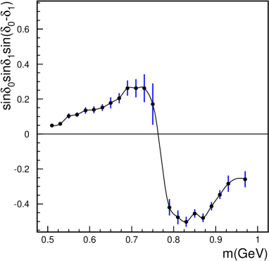
(a)		(b)

Figure 4.5: Two different models of the invariant mass behavior of the $sp$ interference fragmentation function: (a) Jaffe et al. [117], (b) Radici et al. [150].

A different model was applied by Radici et al. [150]: the expected invariant mass behavior turns out to be very different, as shown in Fig. 4.5 (b), and the magnitude of the effect is estimated to be of the order of 1%. For what concerns $pp$ fragmentation functions, at the moment there are no estimates of their magnitude and behavior. However, in general $p$-wave production of two hadrons becomes significant only when they come from the decay of a spin-one resonance. Because of this, we can expect that the invariant mass shape of these functions corresponds to a Breit-Wigner curve peaked at the resonance mass.

If we integrate over $\cos\theta$, with the polar angle ranging from 0 to $\pi$, the only surviving contributions to the cross sections are

$$\operatorname{{\rm\,d}}^{6}\!\sigma_{UU} =\sum_{q}\frac{\alpha^{2}e_{q}^{2}}{\pi sx_{B}y^{2}}\,A(y)\,f_{1}(x_{B})\,D_{1,UU}\bigl{(}z_{h},M_{h}^{2}\bigr{)}$$ (4.42a)

$$\operatorname{{\rm\,d}}^{6}\!\sigma_{LL} =\sum_{q}\frac{\alpha^{2}e_{q}^{2}}{\pi sx_{B}y^{2}}\,\lambda_{e}\,S_{L}\,C(y)\,g_{1}(x_{B})\,D_{1,UU}\bigl{(}z_{h},M_{h}^{2}\bigr{)}$$ (4.42b)

$$\operatorname{{\rm\,d}}^{6}\!\sigma_{UT} =\sum_{q}\frac{\alpha^{2}e_{q}^{2}}{4sx_{B}y^{2}}\,B(y)\,|\bm{S}_{\perp}|\,\frac{\lvert\bm{R}\rvert}{M_{h}}\,\sin(\phi_{R}+\phi_{S})\,h_{1}(x_{B})\,H_{1,UT}^{\sphericalangle\,sp}\bigl{(}z_{h},M_{h}^{2}\bigr{)}.$$ (4.42c)

It is possible to integrate over $\cos\theta$ with the polar angle going from $-\pi/2$ to $\pi/2$. While the first two cross sections vanish, the transverse cross section would turn out to be

$$\operatorname{{\rm\,d}}^{6}\!\sigma_{UT}=\sum_{q}\frac{\alpha^{2}e_{q}^{2}}{4sx_{B}y^{2}}\,B(y)\,|\bm{S}_{\perp}\,|\frac{\lvert\bm{R}\rvert}{M_{h}}\,\sin(\phi_{R}+\phi_{S})\,h_{1}(x_{B})\,\left(H_{1,UT}^{\sphericalangle\,sp}\bigl{(}z_{h},M_{h}^{2}\bigr{)}+\frac{4}{3\pi}H_{1,LT}^{\sphericalangle\,pp}\bigl{(}z_{h},M_{h}^{2}\bigr{)}\right).$$ (4.43)

While the asymmetry in Eq. (4.42c) is almost identical to the one discussed in Ref. 117, the last asymmetry contains a contribution of pure $p$ waves that, as already mentioned, will become particularly relevant when the two hadrons are produced through a spin-one resonance.

4.5 The correlation function $\Delta$ with transverse momentum

We turn now to the correlation functions with the dependence on the transverse momenta, Eqs. (2.57) and (4.10). Consequently, their general decomposition is richer than before. We already know what is the form of the correlation function $\Phi$ [Eq. (2.58)]. For what concerns the correlation function $\Delta$, the inclusion of transverse momentum results in

$${\cal P}_{-}\,\Delta(z,\zeta,M_{h}^{2},\phi_{R},\bm{k}_{T})\,\gamma^{-}=\frac{1}{8\pi}\Biggl{(}D_{1}\bigl{(}z,\zeta,M_{h}^{2},\bm{k}_{T}^{2},\bm{k}_{T}\cdot\bm{R}_{T}\bigr{)}+{\rm i}H_{1}^{\sphericalangle\prime}\bigl{(}z,\zeta,M_{h}^{2},\bm{k}_{T}^{2},\bm{k}_{T}\cdot\bm{R}_{T}\bigr{)}\,\frac{\makebox[0.0pt][l]{\hskip 1.2pt$\sslash$}{R}_{T}}{M_{h}}\\ +{\rm i}H_{1}^{\perp}\bigl{(}z,\zeta,M_{h}^{2},\bm{k}_{T}^{2},\bm{k}_{T}\cdot\bm{R}_{T}\bigr{)}\,\frac{\makebox[0.0pt][l]{$\sslash$}{k}_{T}}{M_{h}}+G_{1}^{\perp}\bigl{(}z,\zeta,M_{h}^{2},\bm{k}_{T}^{2},\bm{k}_{T}\cdot\bm{R}_{T}\bigr{)}\,\frac{\epsilon_{T}^{\mspace{2.0mu}\mu\nu}R_{T\mu}k_{T\nu}}{M_{h}^{2}}\,\gamma_{5}\Biggr{)}\,{\cal P}_{-}.$$ (4.44)

Once again, we can express the correlation function as a matrix in the chirality space of the quark

$$D(z,\zeta,M_{h}^{2},\phi_{R},\bm{k}_{T})_{\chi^{\prime}_{2}\chi^{\phantom{{}^{\prime}}}_{2}}=\frac{1}{8\pi}\begin{pmatrix}D_{1}+\dfrac{\left\lvert\bm{k}_{T}\times\bm{R}_{T}\right\rvert}{M_{h}^{2}}\,G_{1}^{\perp}&{\rm i}\left({\rm e}^{{\rm i}\phi_{R}}\dfrac{\left\lvert\bm{R}_{T}\right\rvert}{M_{h}}\,H_{1}^{\sphericalangle\prime}+{\rm e}^{{\rm i}\phi_{k}}\dfrac{\left\lvert\bm{k}_{T}\right\rvert}{M_{h}}\,H_{1}^{\perp}\right)\\ -{\rm i}\left({\rm e}^{-{\rm i}\phi_{R}}\dfrac{\left\lvert\bm{R}_{T}\right\rvert}{M_{h}}\,H_{1}^{\sphericalangle\prime}+{\rm e}^{-{\rm i}\phi_{k}}\dfrac{\left\lvert\bm{k}_{T}\right\rvert}{M_{h}}\,H_{1}^{\perp}\right)&D_{1}-\dfrac{\left\lvert\bm{k}_{T}\times\bm{R}_{T}\right\rvert}{M_{h}^{2}}\,G_{1}^{\perp}\end{pmatrix}.$$ (4.45)

We can easily obtain positivity bounds on the transverse-momentum dependent functions

$$\frac{\left\lvert\bm{k}_{T}\times\bm{R}_{T}\right\rvert}{M_{h}^{2}}\left\lvert G_{1}^{\perp}\right\rvert \leq D_{1},$$ (4.46)

$$\frac{\left\lvert\bm{R}_{T}\right\rvert^{2}}{M_{h}^{2}}\,\left(H_{1}^{\sphericalangle\prime}\right)^{2}+\frac{\left\lvert\bm{k}_{T}\right\rvert^{2}}{M_{h}^{2}}\,\left(H_{1}^{\perp}\right)^{2}+\frac{2\,\bm{k}_{T}\cdot\bm{R}_{T}}{M_{h}^{2}}\,H_{1}^{\sphericalangle\prime}H_{1}^{\perp} \leq D_{1}^{2}-\frac{\left\lvert\bm{k}_{T}\times\bm{R}_{T}\right\rvert^{2}}{M_{h}^{4}}\,\left(G_{1}^{\perp}\right)^{2},$$ (4.47)

where it is understood that all the functions are dependent on the variables $z,\,\zeta,\,M_{h}^{2},\,\bm{k}_{T}^{2},\,\bm{k}_{T}\cdot\bm{R}_{T}$.

Note that if we integrate over $\bm{k}_{T}$, the fragmentation function $G_{1}^{\perp}$ will disappear, while parts of the functions $H_{1}^{\sphericalangle\prime}$ and $H_{1}^{\perp}$ will merge into a single function, $H_{1}^{\sphericalangle}$, and we will recover the results of Sec. 4.2.

4.6 Cross section and asymmetries with transverse momentum

Prior to integration over the center-of-mass transverse momentum we have the nine-fold cross section

$$\frac{\operatorname{{\rm\,d}}^{9}\!\sigma}{\operatorname{{\rm\,d}}\zeta\operatorname{{\rm\,d}}M_{h}^{2}\operatorname{{\rm\,d}}\phi_{R}\operatorname{{\rm\,d}}z_{h}\operatorname{{\rm\,d}}^{2}\!\bm{P}_{h\perp}\operatorname{{\rm\,d}}x_{B}\operatorname{{\rm\,d}}y\operatorname{{\rm\,d}}\phi_{S}}=\\ \sum_{q}\,\rho(S)_{\Lambda^{\phantom{{}^{\prime}}}_{1}\Lambda_{1}^{\prime}}\;{\cal I}\left[F(x_{B},\bm{p}_{T})_{\chi^{\phantom{{}^{\prime}}}_{1}\chi^{\prime}_{1}}^{\Lambda_{1}^{\prime}\Lambda^{\phantom{{}^{\prime}}}_{1}}\Bigl{(}\frac{\operatorname{{\rm\,d}}\sigma^{eq}}{\operatorname{{\rm\,d}}y}\Bigr{)}^{\chi^{\phantom{{}^{\prime}}}_{1}\chi^{\prime}_{1};\,\chi^{\phantom{{}^{\prime}}}_{2}\chi^{\prime}_{2}}\,D(z_{h},\bm{k}_{T},\zeta,M_{h}^{2},\phi_{R})_{\chi^{\prime}_{2}\chi^{\phantom{{}^{\prime}}}_{2}}\right],$$ (4.48)

To simplify the notation, we introduce the projection $\bm{a}_{T}\wedge\bm{b}_{T}=a_{i}\epsilon_{T}^{ij}b_{j}$. Inserting the formulae obtained for the distribution correlation matrix, Eq. (2.48), the elementary cross section, Eq. (3.21), and the two-hadron fragmentation matrix, Eq. (4.45), we obtain the following result

$$\begin{split}\operatorname{{\rm\,d}}^{9}\!\sigma_{UU}&=\sum_{q}\frac{\alpha^{2}e_{q}^{2}}{2\pi sx_{B}y^{2}}\,\Biggl{\{}A(y)\,{\cal I}\left[f_{1}\,D_{1}\right]-B(y)\,\frac{|{\bm{R}}_{T}|}{M_{h}}\,\cos(\phi_{h}+\phi_{R})\,{\cal I}\left[\frac{\bm{p}_{T}\cdot\hat{\bm{P}}_{h\perp}}{M}\,h_{1}^{\perp}\,H_{1}^{\sphericalangle\prime}\right]\\ &\quad+B(y)\,\frac{|{\bm{R}}_{T}|}{M_{h}}\,\sin(\phi_{h}+\phi_{R})\,{\cal I}\left[\frac{\hat{\bm{P}}_{h\perp}\wedge\bm{p}_{T}}{M}\,h_{1}^{\perp}\,H_{1}^{\sphericalangle\prime}\right]\\ &\quad-B(y)\,\cos(2\phi_{h})\,{\cal I}\left[\frac{2(\bm{p}_{T}\cdot\hat{\bm{P}}_{h\perp})(\bm{k}_{T}\cdot\hat{\bm{P}}_{h\perp})-\bm{p}_{T}\cdot\bm{k}_{T}}{MM_{h}}\,h_{1}^{\perp}\,H_{1}^{\perp}\right]\\ &\quad+B(y)\,\sin(2\phi_{h})\,{\cal I}\left[\frac{(\bm{p}_{T}\cdot\hat{\bm{P}}_{h\perp})(\hat{\bm{P}}_{h\perp}\wedge\bm{k}_{T})+(\bm{k}_{T}\cdot\hat{\bm{P}}_{h\perp})(\hat{\bm{P}}_{h\perp}\wedge\bm{p}_{T})}{MM_{h}}\,h_{1}^{\perp}\,H_{1}^{\perp}\right]\Biggr{\}},\end{split}$$ (4.49)

$$\begin{split}\operatorname{{\rm\,d}}^{9}\!\sigma_{LU}&=-\sum_{q}\frac{\alpha^{2}e_{q}^{2}}{2\pi sx_{B}y^{2}}\,\left\lvert\lambda_{e}\right\rvert\,C(y)\,\frac{|{\bm{R}}_{T}|}{M_{h}}\,\Biggl{\{}\sin(\phi_{h}-\phi_{R})\,{\cal I}\left[\frac{\bm{k}_{T}\cdot\hat{\bm{P}}_{h\perp}}{M_{h}}\,f_{1}\,G_{1}^{\perp}\right]\\ &\quad+\cos(\phi_{h}-\phi_{R})\,{\cal I}\left[\frac{\hat{\bm{P}}_{h\perp}\wedge\bm{k}_{T}}{M_{h}}\,f_{1}\,G_{1}^{\perp}\right]\Biggr{\}},\end{split}$$ (4.50)

$$\begin{split}\operatorname{{\rm\,d}}^{9}\!\sigma_{UL}&=\sum_{q}\frac{\alpha^{2}e_{q}^{2}}{2\pi sx_{B}y^{2}}\,\left\lvert S_{L}\right\rvert\Biggl{\{}-A(y)\,\frac{|{\bm{R}}_{T}|}{M_{h}}\,\sin(\phi_{h}-\phi_{R})\,{\cal I}\left[\frac{\bm{k}_{T}\cdot\hat{\bm{P}}_{h\perp}}{M_{h}}\,g_{1L}\,G_{1}^{\perp}\right]\\ &\quad-A(y)\,\frac{|{\bm{R}}_{T}|}{M_{h}}\,\cos(\phi_{h}-\phi_{R})\,{\cal I}\left[\frac{\hat{\bm{P}}_{h\perp}\wedge\bm{k}_{T}}{M_{h}}\,g_{1L}\,G_{1}^{\perp}\right]\\ &\quad+B(y)\,\frac{|{\bm{R}}_{T}|}{M_{h}}\,\sin(\phi_{h}+\phi_{R})\,{\cal I}\left[\frac{\bm{p}_{T}\cdot\hat{\bm{P}}_{h\perp}}{M}\,h_{1L}^{\perp}\,H_{1}^{\sphericalangle\prime}\right]\\ &\quad+B(y)\,\frac{|{\bm{R}}_{T}|}{M_{h}}\,\cos(\phi_{h}+\phi_{R})\,{\cal I}\left[\frac{\hat{\bm{P}}_{h\perp}\wedge\bm{p}_{T}}{M}\,h_{1L}^{\perp}\,H_{1}^{\sphericalangle\prime}\right]\\ &\quad+B(y)\,\sin(2\phi_{h})\,{\cal I}\left[\frac{2(\bm{p}_{T}\cdot\hat{\bm{P}}_{h\perp})(\bm{k}_{T}\cdot\hat{\bm{P}}_{h\perp})-\bm{p}_{T}\cdot\bm{k}_{T}}{MM_{h}}\,h_{1L}^{\perp}\,H_{1}^{\perp}\right]\\ &\quad+B(y)\,\cos(2\phi_{h})\,{\cal I}\left[\frac{(\bm{p}_{T}\cdot\hat{\bm{P}}_{h\perp})(\hat{\bm{P}}_{h\perp}\wedge\bm{k}_{T})+(\bm{k}_{T}\cdot\hat{\bm{P}}_{h\perp})(\hat{\bm{P}}_{h\perp}\wedge\bm{p}_{T})}{MM_{h}}\,h_{1L}^{\perp}\,H_{1}^{\perp}\right]\Biggr{\}},\end{split}$$ (4.51)

$$\begin{split}\operatorname{{\rm\,d}}^{9}\!\sigma_{LL}&=\sum_{q}\frac{\alpha^{2}e_{q}^{2}}{2\pi sx_{B}y^{2}}\,\left\lvert\lambda_{e}\right\rvert\,\left\lvert S_{L}\right\rvert\,C(y)\,{\cal I}\left[g_{1L}\,D_{1}\right],\end{split}$$ (4.52)

$$\begin{split}\operatorname{{\rm\,d}}^{9}\!\sigma_{UT}&=\sum_{q}\frac{\alpha^{2}e_{q}^{2}}{2\pi sx_{B}y^{2}}\,\left\lvert\bm{S}_{T}\right\rvert\,A(y)\,\Biggl{\{}\frac{|{\bm{R}}_{T}|}{M_{h}}\,\sin(\phi_{R}-\phi_{S})\,{\cal I}\left[\frac{\bm{p}_{T}\cdot\bm{k}_{T}}{2MM_{h}}g_{1T}\,G_{1}^{\perp}\right]\\ &\quad-\frac{|{\bm{R}}_{T}|}{M_{h}}\,\cos(\phi_{R}-\phi_{S})\,{\cal I}\left[\frac{(\bm{p}_{T}\cdot\hat{\bm{P}}_{h\perp})(\hat{\bm{P}}_{h\perp}\wedge\bm{k}_{T})-(\bm{k}_{T}\cdot\hat{\bm{P}}_{h\perp})(\hat{\bm{P}}_{h\perp}\wedge\bm{p}_{T})}{2MM_{h}}g_{1T}\,G_{1}^{\perp}\right]\\ &\quad-\frac{|{\bm{R}}_{T}|}{M_{h}}\,\sin(2\phi_{h}-\phi_{R}-\phi_{S})\,{\cal I}\left[\frac{2(\bm{p}_{T}\cdot\hat{\bm{P}}_{h\perp})(\bm{k}_{T}\cdot\hat{\bm{P}}_{h\perp})-\bm{p}_{T}\cdot\bm{k}_{T}}{2MM_{h}}\,g_{1T}\,G_{1}^{\perp}\right]\\ &\quad-\frac{|{\bm{R}}_{T}|}{M_{h}}\,\cos(2\phi_{h}-\phi_{R}-\phi_{S})\,{\cal I}\left[\frac{(\bm{p}_{T}\cdot\hat{\bm{P}}_{h\perp})(\hat{\bm{P}}_{h\perp}\wedge\bm{k}_{T})+(\bm{k}_{T}\cdot\hat{\bm{P}}_{h\perp})(\hat{\bm{P}}_{h\perp}\wedge\bm{p}_{T})}{2MM_{h}}\,g_{1T}\,G_{1}^{\perp}\right]\\ &\quad+\sin(\phi_{h}-\phi_{S})\,{\cal I}\left[\frac{\bm{p}_{T}\cdot\hat{\bm{P}}_{h\perp}}{M}\,f_{1T}^{\perp}\,D_{1}\right]+\cos(\phi_{h}-\phi_{S})\,{\cal I}\left[\frac{\hat{\bm{P}}_{h\perp}\wedge\bm{p}_{T}}{M}\,f_{1T}^{\perp}\,D_{1}\right]\Biggr{\}}\\ &\quad+\sum_{q}\frac{\alpha^{2}e_{q}^{2}}{2\pi sx_{B}y^{2}}\,\left\lvert\bm{S}_{T}\right\rvert\,B(y)\,\Biggl{\{}\sin(\phi_{h}+\phi_{S})\,{\cal I}\left[\frac{\bm{k}_{T}\cdot\hat{\bm{P}}_{h\perp}}{M_{h}}\,h_{1}\,H_{1}^{\perp}\right]\\ &\quad+\cos(\phi_{h}+\phi_{S})\,{\cal I}\left[\frac{\hat{\bm{P}}_{h\perp}\wedge\bm{k}_{T}}{M_{h}}\,h_{1}\,H_{1}^{\perp}\right]+\frac{|{\bm{R}}_{T}|}{M_{h}}\,\sin(\phi_{R}+\phi_{S})\,{\cal I}\left[h_{1}\,H_{1}^{\sphericalangle\prime}\right]+\sin(3\phi_{h}-\phi_{S})\\ &\quad\times{\cal I}\left[\frac{4(\bm{p}_{T}\cdot\hat{\bm{P}}_{h\perp})^{2}(\bm{k}_{T}\cdot\hat{\bm{P}}_{h\perp})-2(\bm{p}_{T}\cdot\hat{\bm{P}}_{h\perp})(\bm{p}_{T}\cdot\bm{k}_{T})-\bm{p}_{T}^{2}(\bm{k}_{T}\cdot\hat{\bm{P}}_{h\perp})}{2M^{2}M_{h}}\,h_{1T}^{\perp}\,H_{1}^{\perp}\right]\\ &\quad+\cos(3\phi_{h}-\phi_{S})\,{\cal I}\Biggl{[}\Biggl{(}\frac{2(\bm{p}_{T}\cdot\hat{\bm{P}}_{h\perp})^{2}(\hat{\bm{P}}_{h\perp}\wedge\bm{k}_{T})+2(\bm{k}_{T}\cdot\hat{\bm{P}}_{h\perp})(\bm{p}_{T}\cdot\hat{\bm{P}}_{h\perp})(\hat{\bm{P}}_{h\perp}\wedge\bm{p}_{T})}{2M^{2}M_{h}}\\ &\quad-\frac{\bm{p}_{T}^{2}(\hat{\bm{P}}_{h\perp}\wedge\bm{k}_{T})}{2M^{2}M_{h}}\Biggr{)}\,h_{1T}^{\perp}\,H_{1}^{\perp}\Biggr{]}+\frac{|{\bm{R}}_{T}|}{M_{h}}\,\sin(2\phi_{h}+\phi_{R}-\phi_{S})\,{\cal I}\left[\frac{2(\bm{p}_{T}\cdot\hat{\bm{P}}_{h\perp})^{2}-\bm{p}_{T}^{2}}{2M^{2}}\,h_{1T}^{\perp}\,H_{1}^{\sphericalangle\prime}\right]\\ &\quad+\frac{|{\bm{R}}_{T}|}{M_{h}}\,\cos(2\phi_{h}+\phi_{R}-\phi_{S})\,{\cal I}\left[\frac{(\bm{p}_{T}\cdot\hat{\bm{P}}_{h\perp})(\hat{\bm{P}}_{h\perp}\wedge\bm{p}_{T})}{2M^{2}}\,h_{1T}^{\perp}\,H_{1}^{\sphericalangle\prime}\right]\Biggr{\}},\end{split}$$ (4.53)

$$\begin{split}\operatorname{{\rm\,d}}^{9}\!\sigma_{LT}&=\sum_{q}\frac{\alpha^{2}e_{q}^{2}}{2\pi sx_{B}y^{2}}\,\left\lvert\bm{S}_{T}\right\rvert\,C(y)\,\Biggl{\{}\cos(\phi_{h}-\phi_{S})\,{\cal I}\left[\frac{\bm{p}_{T}\cdot\hat{\bm{P}}_{h\perp}}{M}\,g_{1T}\,D_{1}\right]\\ &\quad-\sin(\phi_{h}-\phi_{S})\,{\cal I}\left[\frac{\hat{\bm{P}}_{h\perp}\wedge\bm{p}_{T}}{M}\,g_{1T}\,D_{1}\right]\\ &\quad-\frac{|{\bm{R}}_{T}|}{M_{h}}\,\cos(\phi_{R}-\phi_{S})\,{\cal I}\left[\frac{\bm{p}_{T}\cdot\bm{k}_{T}}{2MM_{h}}f_{1T}^{\perp}\,G_{1}^{\perp}\right]\\ &\quad+\frac{|{\bm{R}}_{T}|}{M_{h}}\,\cos(2\phi_{h}-\phi_{R}-\phi_{S})\,{\cal I}\left[\frac{2(\bm{p}_{T}\cdot\hat{\bm{P}}_{h\perp})(\bm{k}_{T}\cdot\hat{\bm{P}}_{h\perp})-\bm{p}_{T}\cdot\bm{k}_{T}}{2MM_{h}}\,f_{1T}^{\perp}\,G_{1}^{\perp}\right]\\ &\quad-\frac{|{\bm{R}}_{T}|}{M_{h}}\,\sin(\phi_{R}-\phi_{S})\,{\cal I}\left[\frac{(\bm{p}_{T}\cdot\hat{\bm{P}}_{h\perp})(\hat{\bm{P}}_{h\perp}\wedge\bm{k}_{T})-(\bm{k}_{T}\cdot\hat{\bm{P}}_{h\perp})(\hat{\bm{P}}_{h\perp}\wedge\bm{p}_{T})}{2MM_{h}}f_{1T}^{\perp}\,G_{1}^{\perp}\right]\\ &\quad+\frac{|{\bm{R}}_{T}|}{M_{h}}\,\sin(2\phi_{h}-\phi_{R}-\phi_{S})\,{\cal I}\left[\frac{(\bm{p}_{T}\cdot\hat{\bm{P}}_{h\perp})(\hat{\bm{P}}_{h\perp}\wedge\bm{k}_{T})+(\bm{k}_{T}\cdot\hat{\bm{P}}_{h\perp})(\hat{\bm{P}}_{h\perp}\wedge\bm{p}_{T})}{2MM_{h}}\,f_{1T}^{\perp}\,G_{1}^{\perp}\right]\Biggr{\}}.\end{split}$$ (4.54)

4.7 Partial-wave expansion with transverse momentum

To proceed with the partial wave expansion of transverse-momentum dependent functions, it turns out to be convenient to rewrite the correlation function in a somewhat different way, i.e.

$$D(z,\zeta,M_{h}^{2},\phi_{R},\bm{k}_{T})_{\chi^{\prime}_{2}\chi^{\phantom{{}^{\prime}}}_{2}}=\frac{1}{8\pi}\begin{pmatrix}D_{1}+\dfrac{\left\lvert\bm{k}_{T}\times\bm{R}_{T}\right\rvert}{M_{h}^{2}}\,G_{1}^{\perp}&{\rm i}{\rm e}^{{\rm i}\phi_{k}}\,\dfrac{\left\lvert\bm{k}_{T}\right\rvert}{M_{h}}\,H_{1}^{\perp\sphericalangle}\\ -{\rm i}{\rm e}^{-{\rm i}\phi_{k}}\,\dfrac{\left\lvert\bm{k}_{T}\right\rvert}{M_{h}}\,\left(H_{1}^{\perp\sphericalangle}\right)^{\ast}&D_{1}-\dfrac{\left\lvert\bm{k}_{T}\times\bm{R}_{T}\right\rvert}{M_{h}^{2}}\,G_{1}^{\perp}\end{pmatrix}.$$ (4.55)

The functions $H_{1}^{\sphericalangle}$ and $H_{1}^{\perp}$ have been merged into the complex function

$$\begin{split}H_{1}^{\perp\sphericalangle}\left(z,\zeta,M_{h}^{2},\bm{k}_{T}^{2},{\rm e}^{{\rm i}(\phi_{k}-\phi_{R})}\right)&=H_{1}^{\perp}\left(z,\zeta,M_{h}^{2},\bm{k}_{T}^{2},\cos(\phi_{k}-\phi_{R})\right)\\ &\quad+{\rm e}^{{\rm i}(\phi_{R}-\phi_{k})}\,H_{1}^{\sphericalangle}\left(z,\zeta,M_{h}^{2},\bm{k}_{T}^{2},\cos(\phi_{k}-\phi_{R})\right).\end{split}$$ (4.56)

Because of the presence of the azimuthal angles, this function can be expanded in spherical harmonics, provided we retain only those terms which are consistent with the definition in Eq. (4.56). If we wish to include only the $s$- and $p$-wave contributions, the partial wave expansion of the function $H_{1}^{\perp\sphericalangle}$ takes the form

$$\begin{split}H_{1}^{\perp\sphericalangle}&=H_{1,UU}^{\perp}+H_{1,UL}^{\perp\,sp}\cos{\theta}+H_{1,LL}^{\perp\,pp}\,\frac{1}{4}\left(3\cos^{2}{\theta}-1\right)+{\rm e}^{{\rm i}(\phi_{k}-\phi_{R})}\sin\theta\left(H_{1,UT}^{\perp\,sp}+H_{1,LT}^{\perp\,pp}\cos{\theta}\right)\\ &\quad+{\rm e}^{-{\rm i}(\phi_{k}-\phi_{R})}\sin\theta\left(H_{1,UT}^{\perp\,sp}+H_{1,LT}^{\perp\,pp}\cos{\theta}+\frac{\lvert\bm{R}\rvert}{\left\lvert\bm{k}_{T}\right\rvert}\,H_{1,UT}^{\sphericalangle\,sp\prime}+\frac{\lvert\bm{R}\rvert}{\left\lvert\bm{k}_{T}\right\rvert}\,H_{1,LT}^{\sphericalangle\,pp\prime}\cos{\theta}\right)\\ &\quad+{\rm e}^{2{\rm i}(\phi_{k}-\phi_{R})}\sin^{2}\theta\,H_{1,TT}^{\perp\,pp}+{\rm e}^{-2{\rm i}(\phi_{k}-\phi_{R})}\sin^{2}\theta\left(H_{1,TT}^{\perp\,pp}+\frac{\lvert\bm{R}\rvert}{\left\lvert\bm{k}_{T}\right\rvert}\,H_{1,TT}^{\sphericalangle\,pp}\right)\end{split}$$ (4.57)

Note that the functions on the right-hand side depend only on the variables $z$, $M_{h}^{2}$, $\bm{k}_{T}^{2}$.

The expansion of the other two functions, $D_{1}$ and $G_{1}^{\perp}$, is considerably simpler, because they can depend only on $\cos(\phi_{h}-\phi_{R})$

$$D_{1} =D_{1,UU}+D_{1,UL}^{sp}\cos{\theta}+D_{1,LL}^{pp}\,\frac{1}{4}\left(3\cos^{2}{\theta}-1\right)+\cos(\phi_{k}-\phi_{R})\,\sin{\theta}\left(D_{1,UT}^{\perp\,sp}+D_{1,LT}^{\perp\,pp}\cos{\theta}\right)$$

$$\quad+\cos(2\phi_{k}-2\phi_{R})\,\sin^{2}\theta\,D_{1,TT}^{\perp\,pp},$$ (4.58a)

$$G_{1}^{\perp} =G_{1,UT}^{\perp\,sp}+G_{1,LT}^{\perp\,pp}\cos{\theta}+\cos(\phi_{k}-\phi_{R})\,\sin{\theta}\,G_{1,TT}^{\perp\,pp},$$ (4.58b)

where the functions on the right-hand side depend only on the variables $z$, $M_{h}^{2}$, $\bm{k}_{T}^{2}$.

As a conclusive remark, note that it would have been possible to expand the functions $H_{1}^{\sphericalangle}$ and $H_{1}^{\perp}$ in a way similar to what we have done for $D_{1}$ and $G_{1}^{\perp}$, but some care is required to properly treat the component $H_{1,TT}^{\sphericalangle\,pp}$, which is shared by the two functions. This is why we preferred to take an alternative way. In any case, for completeness we give also the expansions of $H_{1}^{\sphericalangle}$ and $H_{1}^{\perp}$ separately:

$$H_{1}^{\perp} =H_{1,UU}^{\perp}+H_{1,UL}^{\perp\,sp}\cos{\theta}+H_{1,LL}^{\perp\,pp}\,\frac{1}{4}\left(3\cos^{2}{\theta}-1\right)+2\cos(\phi_{k}-\phi_{R})\,\sin{\theta}\left(H_{1,UT}^{\perp\,sp}+H_{1,LT}^{\perp\,pp}\cos{\theta}\right)$$

$$\quad+2\cos(2\phi_{k}-2\phi_{R})\,\sin^{2}\theta\,H_{1,TT}^{\perp\,pp}-\sin^{2}\theta\,\frac{\lvert\bm{R}\rvert}{\lvert\bm{k}_{T}\rvert}\,H_{1,TT}^{\sphericalangle\,pp},$$ (4.59a)

$$H_{1}^{\sphericalangle} =H_{1,UT}^{\sphericalangle\,sp\prime}+H_{1,LT}^{\sphericalangle\,pp\prime}\cos{\theta}+2\cos(\phi_{k}-\phi_{R})\,\sin{\theta}\,H_{1,TT}^{\sphericalangle\,pp}.$$ (4.59b)

As before, the functions on the right-hand side depend only on the variables $z$, $M_{h}^{2}$, $\bm{k}_{T}^{2}$.

As we have done in Sec. 4.4.2, it is possible to rewrite the correlation function as a trace between the decay matrix, Eq. (4.32), and a fragmentation matrix in the quark chirality space $\otimes$ the hadronic system angular momentum space

$$D(z,\cos\theta,M_{h}^{2},\phi_{R},\bm{k}_{T})_{\chi^{\prime}_{2}\chi^{\phantom{{}^{\prime}}}_{2}}=D(z,M_{h}^{2},\bm{k}_{T}^{2})_{\chi^{\prime}_{2}\chi^{\phantom{{}^{\prime}}}_{2}}^{j^{\prime}m^{\prime},jm}{\cal D}_{jm,j^{\prime}m^{\prime}}(\theta,\phi_{R}).$$ (4.60)

Once again, the result is a $8\times 8$ matrix

$$D(z,M_{h}^{2},\bm{k}_{T}^{2})_{\chi^{\prime}_{2}\chi^{\phantom{{}^{\prime}}}_{2}}^{j^{\prime}m^{\prime},jm}=\frac{1}{8}\begin{pmatrix}A_{j^{\prime}m^{\prime},jm}&B_{j^{\prime}m^{\prime},jm}\\ B_{j^{\prime}m^{\prime},jm}^{\dagger}&C_{j^{\prime}m^{\prime},jm}\end{pmatrix}.$$ (4.61)

The inner blocks span the space of the orbital angular momentum of the hadronic system and read

$$A_{j^{\prime}m^{\prime},jm}=\\ \left(\begin{array}[]{>{\scriptstyle}c|>{\scriptstyle}c>{\scriptstyle}c>{\scriptstyle}c}D_{1,UU}^{ss}&-\sqrt{\frac{2}{3}}{\rm e}^{{\rm i}\phi}\left(D_{1,UT}^{\perp\,sp}+{\rm i}\frac{\lvert\bm{k}_{T}\rvert\lvert\bm{R}\rvert}{M_{h}^{2}}G_{1,UT}^{\perp\,sp}\right)&\frac{2}{\sqrt{3}}D_{1,UL}^{sp}&\sqrt{\frac{2}{3}}{\rm e}^{-{\rm i}\phi}\left(D_{1,UT}^{\perp\,sp}-{\rm i}\frac{\lvert\bm{k}_{T}\rvert\lvert\bm{R}\rvert}{M_{h}^{2}}G_{1,UT}^{\perp\,sp}\right)\\[3.0pt] \hline\cr-\sqrt{\frac{2}{3}}{\rm e}^{-{\rm i}\phi}\left(D_{1,UT}^{\perp\,sp}-{\rm i}\frac{\lvert\bm{k}_{T}\rvert\lvert\bm{R}\rvert}{M_{h}^{2}}G_{1,UT}^{\perp\,sp}\right)&D_{1,UU}^{pp}-\frac{1}{3}D_{1,LL}^{pp}&-\frac{\sqrt{2}}{3}{\rm e}^{-{\rm i}\phi}\left(D_{1,LT}^{\perp\,pp}-{\rm i}\frac{\lvert\bm{k}_{T}\rvert\lvert\bm{R}\rvert}{M_{h}^{2}}G_{1,LT}^{\perp\,pp}\right)&-\frac{2}{3}{\rm e}^{-2{\rm i}\phi}\left(2D_{1,TT}^{\perp\,pp}-{\rm i}\frac{\lvert\bm{k}_{T}\rvert\lvert\bm{R}\rvert}{M_{h}^{2}}G_{1,TT}^{\perp\,pp}\right)\\ \frac{2}{\sqrt{3}}D_{1,UL}^{sp}&-\frac{\sqrt{2}}{3}{\rm e}^{{\rm i}\phi}\left(D_{1,LT}^{\perp\,pp}+{\rm i}\frac{\lvert\bm{k}_{T}\rvert\lvert\bm{R}\rvert}{M_{h}^{2}}G_{1,LT}^{\perp\,pp}\right)&D_{1,UU}^{pp}+\frac{2}{3}D_{1,LL}^{pp}&\frac{\sqrt{2}}{3}{\rm e}^{-{\rm i}\phi}\left(D_{1,LT}^{\perp\,pp}-{\rm i}\frac{\lvert\bm{k}_{T}\rvert\lvert\bm{R}\rvert}{M_{h}^{2}}G_{1,LT}^{\perp\,pp}\right)\\ \sqrt{\frac{2}{3}}{\rm e}^{{\rm i}\phi}\left(D_{1,UT}^{\perp\,sp}+{\rm i}\frac{\lvert\bm{k}_{T}\rvert\lvert\bm{R}\rvert}{M_{h}^{2}}G_{1,UT}^{\perp\,sp}\right)&-\frac{2}{3}{\rm e}^{2{\rm i}\phi}\left(2D_{1,TT}^{\perp\,pp}+{\rm i}\frac{\lvert\bm{k}_{T}\rvert\lvert\bm{R}\rvert}{M_{h}^{2}}G_{1,TT}^{\perp\,pp}\right)&\frac{\sqrt{2}}{3}{\rm e}^{{\rm i}\phi}\left(D_{1,LT}^{\perp\,pp}+{\rm i}\frac{\lvert\bm{k}_{T}\rvert\lvert\bm{R}\rvert}{M_{h}^{2}}G_{1,LT}^{\perp\,pp}\right)&D_{1,UU}^{pp}-\frac{1}{3}D_{1,LL}^{pp}\end{array}\right),$$

$$B_{j^{\prime}m^{\prime},jm}={\rm i}\frac{\lvert\bm{k}_{T}\rvert}{M_{h}}\left(\begin{array}[]{>{\scriptstyle}c|>{\scriptstyle}c>{\scriptstyle}c>{\scriptstyle}c}{\rm e}^{{\rm i}\phi}H_{1,UU}^{\perp\,ss}&-\frac{4}{\sqrt{6}}{\rm e}^{2{\rm i}\phi}H_{1,UT}^{\perp\,sp}&\frac{2}{\sqrt{3}}{\rm e}^{{\rm i}\phi}H_{1,UL}^{\perp\,sp}&\frac{4}{\sqrt{6}}\left(\frac{\lvert\bm{R}\rvert}{\lvert\bm{k}_{T}\rvert}H_{1,UT}^{\sphericalangle\,sp\prime}+H_{1,UT}^{\perp\,sp}\right)\\[3.0pt] \hline\cr-\frac{4}{\sqrt{6}}\left(\frac{\lvert\bm{R}\rvert}{\lvert\bm{k}_{T}\rvert}H_{1,UT}^{\sphericalangle\,sp\prime}+H_{1,UT}^{\perp\,sp}\right)&{\rm e}^{{\rm i}\phi}\left(H_{1,UU}^{\perp\,pp}-\frac{1}{3}H_{1,LL}^{\perp\,pp}\right)&-\frac{2\sqrt{2}}{3}\left(\frac{\lvert\bm{R}\rvert}{\lvert\bm{k}_{T}\rvert}H_{1,LT}^{\sphericalangle\,pp\prime}+H_{1,LT}^{\perp\,pp}\right)&-\frac{8}{3}{\rm e}^{-{\rm i}\phi}\left(\frac{\lvert\bm{R}\rvert}{\lvert\bm{k}_{T}\rvert}H_{1,TT}^{\sphericalangle\,pp}+H_{1,TT}^{\perp\,pp}\right)\\ \frac{2}{\sqrt{3}}{\rm e}^{{\rm i}\phi}H_{1,UL}^{\perp\,sp}&-\frac{2\sqrt{2}}{3}{\rm e}^{2{\rm i}\phi}H_{1,LT}^{\perp\,pp}&{\rm e}^{{\rm i}\phi}\left(H_{1,UU}^{\perp\,pp}+\frac{2}{3}H_{1,LL}^{\perp\,pp}\right)&\frac{2\sqrt{2}}{3}\left(\frac{\lvert\bm{R}\rvert}{\lvert\bm{k}_{T}\rvert}H_{1,LT}^{\sphericalangle\,pp\prime}+H_{1,LT}^{\perp\,pp}\right)\\ \frac{4}{\sqrt{6}}{\rm e}^{2{\rm i}\phi}H_{1,UT}^{\perp\,sp}&-\frac{8}{3}{\rm e}^{3{\rm i}\phi}H_{1,TT}^{\perp\,pp}&\frac{2\sqrt{2}}{3}{\rm e}^{2{\rm i}\phi}H_{1,LT}^{\perp\,pp}&{\rm e}^{{\rm i}\phi}\left(H_{1,UU}^{\perp\,pp}-\frac{1}{3}H_{1,LL}^{\perp\,pp}\right)\end{array}\right).$$

The block $C$ of the fragmentation matrix can be obtained from the block $A$ by imposing parity invariance relations.

The $ss$ sector of the matrix contains functions analogous to the ones we discussed in the previous chapter in the context of single-particle unpolarized fragmentation. The $pp$ sector corresponds to the spin-one fragmentation functions studied in Ref. 36. We will discuss them again in the next chapter. The $sp$ interference sector has never been studied with the inclusion of transverse momentum.

Similar considerations to the ones discussed after Eqs. (4.35) hold for the transverse momentum dependent fragmentation matrix. In particular, the matrix fulfills the properties of Hermiticity, conservation of angular momentum ($m+\chi^{\prime}_{2}=m^{\prime}+\chi_{2}+l$) and parity invariance

$$D_{\chi^{\prime}_{2}\chi^{\phantom{{}^{\prime}}}_{2}}^{j^{\prime}m^{\prime},jm}=(-1)^{l}D_{{-\chi^{\prime}_{2}}\,{-\chi^{\phantom{{}^{\prime}}}_{2}}}^{j^{\prime}\,{-m^{\prime}},j\;{-m}}.$$ (4.62)

The imaginary parts of the matrix represent T-odd functions. Note that the off-diagonal blocks, which are chiral-odd, can only contain T-odd functions. The matrix could in principle contain other functions, but they are lost when tracing with the decay matrix and thus cannot be analyzed by a parity conserving decay process.

From the fact that the matrix $D(z,M_{h}^{2},\bm{k}_{T}^{2})$ is positive semi-definite, it is possible to obtain positivity bounds on the fragmentation functions, as we have done already before.

4.8 Summary

In this chapter we analyzed two-particle inclusive deep inelastic scattering, at leading order in $1/Q$, without and with partonic transverse momentum. For the description of the fragmentation side, we introduced a correlation function $\Delta$ that depends on the center-of-mass momentum of the two hadrons and on their relative momentum.

In the first part of the chapter we neglected partonic transverse momentum. We distinguished one chiral-even T-even and one chiral-odd T-odd fragmentation function [Eq. (4.14)]. They are complicated objects depending on three variables, whereas single-particle fragmentation functions depend on one variable only. We derived positivity bounds on these functions [Eqs. (4.18)] and we computed the cross section of two-particle inclusive scattering [Eq. (4.20)].

Since two-particle systems with a low invariant mass are usually produced in the $s$ and $p$ waves, we performed a partial wave expansion of the fragmentation functions taking into consideration only these two lowest modes. We split the chiral-even fragmentation function into three contributions, pertaining to the pure $s$ waves, pure $p$ waves and $sp$ interference. We split the chiral-odd function into two contributions, typical of pure $p$ waves and $sp$ interference. These five new fragmentation functions depend only on two variables, namely $z$ and the invariant mass squared of the system [Eq. (4.30)]. Employing the usual helicity formalism, we discussed positivity bounds on the new fragmentation functions [Eqs. (4.38) and (4.39)]. We computed all non vanishing spin asymmetries of two-particle inclusive DIS at leading twist [Eqs. (4.41)]. In particular, we showed that in the single transverse spin asymmetry of Eq. (4.41c) the transversity distribution appears in connection with both chiral-odd fragmentation functions. Integrating the asymmetry over different ranges of the polar angle $\theta$, we presented two distinct ways to access the transversity distribution. The first one [Eq. (4.42c)] involves only the $sp$ interference term and corresponds to the one discussed in Ref. 117, while the second one [Eq. (4.43)] involves also the pure $p$ term, which could have an entirely different physical origin and should be particularly relevant in the presence of a spin-one resonance. These two asymmetries are in all respects two distinct ways to access the transversity distribution function. The second one has never been clearly indicated in the literature.

In the rest of the chapter, we repeated the analysis of the correlation function including partonic transverse momentum and also in this case we applied a partial wave expansion.

Chapter 5 Spin one

In the previous chapter we examined the production of two hadrons in the $s$ and $p$ waves. As we already mentioned, the $p$-wave sector of the analysis should overlap with the description of the fragmentation functions for spin-one mesons. The reason is that the polarization of the vector meson can be analyzed by measuring its decay in two other particles, as in the case of a $\rho$ meson decaying into two pions.

In this chapter, we will take a small detour from the mainstream of the thesis, and we shall deal with spin-one targets and spin-one fragments. In the first part, we will examine what is necessary for the description of a spin-one object and what are the differences with the spin-half case. We will introduce distribution functions for quarks inside spin-one objects, with and without transverse momentum.

Then we will turn our attention to spin-one hadrons in the final state and we will examine the fragmentation functions for a quark producing a spin-one hadron. In the end, we will check whether the connection with two-hadron fragmentation can be established and if there are any differences between the two situations.

5.1 Spin-one targets

In recent years some attention has been devoted to distribution functions characterizing spin-one targets, starting from the work of Hoodbhoy, Jaffe and Manohar [110]. Unfortunately, the only available spin-one target is the deuteron, which is essentially a weakly bound system of two spin-half hadrons. In fact, deuteron targets are often used in deep inelastic scattering with the major purpose of extracting the neutron distribution functions. However, the spin-one structure of the deuteron in itself can be very interesting [144, 62, 89, 169]. A large amount of work is already present on deuteron structure functions, especially in Drell-Yan processes [106, 108].

5.1.1 Spin density matrix and spin tensor

The description of particles with spin can be attained by using a spin density matrix ${\bm{\rho}}$ in the rest frame of the particle. The parametrization of the density matrix for a spin-$J$ particle is conveniently performed with the introduction of irreducible spin tensors up to rank $2J$. For example, we have already seen [cf. Eq. (2.42)] that the density matrix of a spin-half particle can be decomposed on a Cartesian basis of $2\times 2$ matrices, formed by the identity matrix and the three Pauli matrices,

$${\bm{\rho}}=\frac{1}{2}\left(\mbox{\bf 1}+S^{i}{\bm{\sigma}}^{i}\right),$$ (5.1)

where we introduced the (rank-one) spin vector $S^{i}$.

To parametrize the density matrix of a spin-one particle we can choose a Cartesian basis of $3\times 3$ matrices, formed by the identity matrix, three spin matrices ${{\bm{\Sigma}}}^{i}$ (generalization of the Pauli matrices to the three-dimensional case) and five extra matrices ${{\bm{\Sigma}}}^{ij}$. These last ones can be built using bilinear combinations of the spin matrices. In three dimensions these combinations are no longer dependent on the spin matrices themselves, as would be for the Pauli matrices. We choose them to be (see Refs. 64, 134 and 42 for a comparison)

$${{\bm{\Sigma}}}^{ij}=\frac{1}{2}\left({{\bm{\Sigma}}}^{i}{{\bm{\Sigma}}}^{j}+{{\bm{\Sigma}}}^{j}{{\bm{\Sigma}}}^{i}\right)-\frac{2}{3}\,{\bf 1}\;\delta^{ij}.$$ (5.2)

With these preliminaries, we can write the spin density matrix as

$${\bm{\rho}}=\frac{1}{3}\left({\bf 1}+\frac{3}{2}\,S^{i}{{\bm{\Sigma}}}^{i}+3\,T^{ij}{{\bm{\Sigma}}}^{ij}\right),$$ (5.3)

where we introduced the symmetric traceless rank-two spin tensor $T^{ij}$. We choose the following way of parametrizing the spin vector and tensor in the rest frame of the hadron,

$${\bm{S}} =\left(S_{T}^{x},S_{T}^{y},S_{L}\right),$$ (5.4a)

$${\bm{T}} =\frac{1}{2}\left(\begin{array}[]{ccc}{S_{LL}}+{S_{TT}^{xx}}&{S_{TT}^{xy}}&{S_{LT}^{x}}\\ {S_{TT}^{xy}}&{S_{LL}}-{S_{TT}^{xx}}&{S_{LT}^{y}}\\ {S_{LT}^{x}}&{S_{LT}^{y}}&-2{S_{LL}}\\ \end{array}\right).$$ (5.4e)

The parameter $S_{LL}$ is often called alignment [64, 134, 91, 93].

Although we introduced the spin vector and tensor in the particle rest frame, it is possible to introduce covariant generalizations of them, satisfying the conditions $P_{\mu}S^{\mu}=0$ and $P_{\mu}T^{\mu\nu}=0$, where $P_{\mu}$ is the momentum of the hadron. In a collinear frame, the parametrizations of the covariant spin vector and tensor will be

$$S^{\mu} =\biggl{[}-S_{L}\,\frac{M}{2P^{+}},\;S_{L}\,\frac{P^{+}}{M},\;\bm{S}_{T}\biggr{]},$$ (5.5a)

$$T^{\mu\nu} =\frac{1}{2}\begin{bmatrix}-S_{LL}\frac{M^{2}}{2(P^{+})^{2}}&S_{LL}&-S_{LT}^{x}\frac{M}{2P^{+}}&-S_{LT}^{y}\frac{M}{2P^{+}}\\ S_{LL}&-2S_{LL}\frac{(P^{+})^{2}}{M^{2}}&S_{LT}^{x}\frac{P^{+}}{M}&S_{LT}^{y}\frac{P^{+}}{M}\\ -S_{LT}^{x}\frac{M}{2P^{+}}&S_{LT}^{x}\frac{P^{+}}{M}&S_{TT}^{xx}+S_{LL}&S_{TT}^{xy}\\ -S_{LT}^{y}\frac{M}{2P^{+}}&S_{LT}^{y}\frac{P^{+}}{M}&S_{TT}^{xy}&-S_{TT}^{xx}+S_{LL}\\ \end{bmatrix}.$$ (5.5b)

In the particle rest frame (where $P^{+}=M/\sqrt{2}$) they correspond to Eqs. (5.4) (note that here they are written in light-cone coordinates).

Inserting in Eq. (5.3) the spin vector, Eq. (5.4a), and the spin tensor, Eq. (5.4e), the explicit form of the spin density matrix $\rho$ turns out to be

$${\bm{\rho}}=\left(\begin{array}[]{ccc}\frac{1}{3}-\frac{S_{LL}}{2}+\frac{S_{L}}{2}&\frac{S_{LT}^{x}-{\rm i}S_{LT}^{y}}{2\sqrt{2}}+\frac{S_{T}^{x}-{\rm i}S_{T}^{y}}{2\sqrt{2}}&\frac{S_{TT}^{xx}-{\rm i}S_{TT}^{xy}}{2}\\ \frac{S_{LT}^{x}+{\rm i}S_{LT}^{y}}{2\sqrt{2}}+\frac{S_{T}^{x}+{\rm i}S_{T}^{y}}{2\sqrt{2}}&\frac{1}{3}+S_{LL}&-\frac{S_{LT}^{x}-{\rm i}S_{LT}^{y}}{2\sqrt{2}}+\frac{S_{T}^{x}-{\rm i}S_{T}^{y}}{2\sqrt{2}}\\ \frac{S_{TT}^{xx}+{\rm i}S_{TT}^{xy}}{2}&-\frac{S_{LT}^{x}+{\rm i}S_{LT}^{y}}{2\sqrt{2}}+\frac{S_{T}^{x}+{\rm i}S_{T}^{y}}{2\sqrt{2}}&\frac{1}{3}-\frac{S_{LL}}{2}-\frac{S_{L}}{2}\end{array}\right).$$ (5.6)

The treatment of spin-one particles can be done equivalently by introducing the complex polarization vector $\bm{\epsilon}$, and its covariant generalization $\epsilon^{\mspace{2.0mu}\mu}$. The two formalisms can be related by means of the formulae [134]

$$\bm{S} =\operatorname{\,{\rm Im}\,}\left(\bm{\epsilon}^{\ast}\times\bm{\epsilon}\right), T_{ij} =\frac{1}{3}\delta_{ij}-\operatorname{\,{\rm Re}\,}\left(\epsilon^{\ast}_{i}\epsilon_{j}\right),$$ (5.7)

or for the covariant generalizations

$$S_{\mu} =-\epsilon_{\mu\alpha\beta\gamma}P^{\alpha}\operatorname{\,{\rm Im}\,}\left(\epsilon^{\ast\beta}\epsilon^{\gamma}\right), T_{\mu\nu} =-\operatorname{\,{\rm Re}\,}\left(\epsilon^{\ast}_{\mu}\epsilon_{\nu}\right)-\frac{1}{3}\left(g_{\mu\nu}-\frac{P_{\mu}P_{\nu}}{P^{2}}\right)\delta_{ij}.$$ (5.8)

5.1.2 Interpretation of the components of the spin tensor

A particular component of the spin tensor measures a combination of probabilities of finding the system in a certain spin state (defined in the particle rest frame). As “analyzing” spin states we can choose the eigenstates of the spin vector operator in a particular direction. We can write the spin vector operator in terms of polar and azimuthal angles,

$${{\bm{\Sigma}}}^{i}\hat{n}_{i}={{\bm{\Sigma}}}_{x}\cos{\vartheta}\cos{\varphi}+{{\bm{\Sigma}}}_{y}\cos{\vartheta}\sin{\varphi}+{{\bm{\Sigma}}}_{z}\sin{\vartheta},$$ (5.9)

and we can denote its eigenstates as $\;\raisebox{-3.0pt}{\rule{0.7pt}{12.0pt}}\,{m,(\vartheta,\varphi)}\bigr{\rangle}$, $m$ being their magnetic quantum number. The probability of finding one of these states can be calculated as

$${\cal P}\left[m,(\vartheta,\varphi)\right]=\operatorname{Tr}\left\{{\bm{\rho}}\,\;\raisebox{-3.0pt}{\rule{0.7pt}{12.0pt}}\,{m,(\vartheta,\varphi)}\bigr{\rangle}\bigl{\langle}{m,(\vartheta,\varphi)}\mspace{2.0mu}\raisebox{-3.0pt}{\rule{0.7pt}{12.0pt}}\;\right\}.$$ (5.10)

From the explicit formula of the density matrix, Eq. (5.6), one can compute

$$S_{LL}=-\tfrac{1}{3}\,{\cal P}\bigl{[}1,{(0,0)}\bigr{]}-\tfrac{1}{3}\,{\cal P}\bigl{[}-1,{(0,0)}\bigr{]}+\tfrac{2}{3}\,{\cal P}\bigl{[}0,{(0,0)}\bigr{]},$$ (5.11a)

$$\begin{aligned} S_{LT}^{x}&={\cal P}\left[0,{\bigl{(}-\tfrac{\pi}{4},0\bigr{)}}\right]-{\cal P}\left[0,{\bigl{(}\tfrac{\pi}{4},0\bigr{)}}\right],&S_{LT}^{y}&={\cal P}\left[0,{\bigl{(}-\tfrac{\pi}{4},\tfrac{\pi}{2}\bigr{)}}\right]-{\cal P}\left[0,{\bigl{(}\tfrac{\pi}{4},\tfrac{\pi}{2}\bigr{)}}\right],\\ S_{TT}^{xx}&={\cal P}\left[0,{\bigl{(}\tfrac{\pi}{2},-\tfrac{\pi}{4}\bigr{)}}\right]-{\cal P}\left[0,{\bigl{(}\tfrac{\pi}{2},\tfrac{\pi}{4}\bigr{)}}\right],&S_{TT}^{xy}&={\cal P}\left[0,{\bigl{(}\tfrac{\pi}{2},\tfrac{\pi}{2}\bigr{)}}\right]-{\cal P}\left[0,{\bigl{(}\tfrac{\pi}{2},0\bigr{)}}\right].\end{aligned}$$ (5.11b)

Below, we suggest a diagrammatic interpretation of these probability combinations. Arrows represent spin states $m=+1$ and $m=-1$ in the direction of the arrow itself, while dashed lines denote spin state $m=0$ in the direction of the line itself.

$$S_{LL}=$$

$$S_{LT}^{x}=\makebox[113.81102pt][c]{\parbox[c]{99.58464pt}{\includegraphics[width=99.58464pt]{Figures/Txz}}} S_{LT}^{y}=\parbox[c]{113.81102pt}{\includegraphics[width=113.81102pt]{Figures/Tyz}}$$

$$S_{TT}^{xy}=\makebox[113.81102pt][c]{\parbox[c]{85.35826pt}{\includegraphics[width=85.35826pt]{Figures/Txy}}} S_{TT}^{xx}=\makebox[113.81102pt][c]{\parbox[c]{85.35826pt}{\includegraphics[width=85.35826pt]{Figures/Txx}}}.$$

The probabilistic interpretations suggest straightforward bounds on the values the spin tensor parameters can achieve, namely

$$-\frac{1}{3} \leq S_{LL}\leq\frac{2}{3}, -1 \leq S_{LT}^{i}\leq 1, -1\leq S_{TT}^{ij}\leq 1,$$ (5.12)

where $i,j=x,y$. Finally, it is possible to define a total degree of polarization

$$\begin{split}d&=\sqrt{\frac{3}{4}\,S^{i}S_{i}+\frac{3}{2}\,T^{ij}T_{ij}}\\ &=\left\{\frac{3}{4}\left[S_{L}^{2}+(S_{T}^{x})^{2}+(S_{T}^{y})^{2}\right]+\frac{3}{4}\left[3\,S_{LL}^{2}+(S_{LT}^{x})^{2}+(S_{LT}^{y})^{2}+(S_{TT}^{xx})^{2}+(S_{TT}^{xy})^{2}\right]\right\}^{1/2},\end{split}$$ (5.13)

whose value ranges between 0 and 1.

5.2 The correlation function $\Phi$

The correlation function $\Phi$ has to fulfill the condition of Hermiticity and parity invariance. For spin-one hadrons, they are slightly different from the spin-half case, because of the presence of the spin tensor

Hermiticity: $$\Phi(p,P,S) =\gamma^{0}\Phi^{{\dagger}}(p,P,S,T)\gamma^{0},$$ (5.14a)

parity: $$\Phi(p,P,S) =\gamma^{0}\Phi(\tilde{p},\tilde{P},-\tilde{S},\tilde{T})\gamma^{0}$$ (5.14b)

where $\tilde{p}^{\nu}=\delta^{\nu\mu}p_{\mu}$ and so forth for the other vectors, and $\tilde{T}^{\mu\nu}=\delta^{\mu\sigma}\delta^{\nu\rho}T_{\sigma\rho}$.

The most general decomposition of the correlation function $\Phi$ for spin-one hadrons is

$$\begin{split}\Phi(p,P,S,T)&=M\,A_{1}\,{\bm{1}}+A_{2}\,\makebox[0.0pt][l]{\hskip 1.2pt$\sslash$}{P}+A_{3}\,\makebox[0.0pt][l]{\hskip 1.3pt$\sslash$}{p}+\left(\frac{A_{4}}{M}\,\sigma_{\mu\nu}P^{\mu}p^{\nu}\right)+\left({\rm i}A_{5}\;p\cdot S\,\gamma_{5}\right)\\ &+M\,A_{6}\,\makebox[0.0pt][l]{\hskip 0.5pt$\sslash$}{S}\,\gamma_{5}+A_{7}\,\frac{p\cdot S}{M}\,\makebox[0.0pt][l]{\hskip 1.2pt$\sslash$}{P}\,\gamma_{5}+A_{8}\,\frac{p\cdot S}{M}\,\makebox[0.0pt][l]{\hskip 1.3pt$\sslash$}{p}\,\gamma_{5}+{\rm i}A_{9}\,\sigma_{\mu\nu}\gamma_{5}S^{\mu}P^{\nu}\\ &+{\rm i}A_{10}\,\sigma_{\mu\nu}\gamma_{5}\,S^{\mu}p^{\nu}+{\rm i}A_{11}\,\frac{p\cdot S}{M^{2}}\,\sigma_{\mu\nu}\gamma_{5}P^{\mu}p^{\nu}+\left(A_{12}\,\frac{\epsilon_{\mu\nu\rho\sigma}\gamma^{\mu}P^{\nu}p^{\rho}S^{\sigma}}{M}\right)\\ &+\frac{A_{13}}{M}\,p_{\mu}p_{\nu}T^{\mu\nu}\,{\bm{1}}+\frac{A_{14}}{M^{2}}\;p_{\mu}p_{\nu}T^{\mu\nu}\makebox[0.0pt][l]{\hskip 1.2pt$\sslash$}{P}+\frac{A_{15}}{M^{2}}\;p_{\mu}p_{\nu}T^{\mu\nu}\makebox[0.0pt][l]{\hskip 1.3pt$\sslash$}{p}\\ &+\left(\frac{A_{16}}{M^{3}}\;p_{\mu}p_{\nu}T^{\mu\nu}\sigma_{\rho\sigma}P^{\rho}p^{\sigma}\right)+A_{17}\;p_{\mu}T^{\mu\nu}\gamma_{\nu}+\left(\frac{A_{18}}{M}\,\sigma_{\nu\rho}P^{\rho}\,p_{\mu}T^{\mu\nu}\right)\\ &+\left(\frac{A_{19}}{M}\,\sigma_{\nu\rho}p^{\rho}p_{\mu}T^{\mu\nu}\right)+\left(\frac{A_{20}}{M^{2}}\,\epsilon_{\mu\nu\rho\sigma}\gamma^{\mu}\gamma_{5}P^{\nu}p^{\rho}\,p_{\tau}T^{\tau\sigma}\right).\end{split}$$ (5.15)

The amplitudes $A_{i}$ are real functions $A_{i}=A_{i}(p\cdot P,p^{2})$. The terms with the amplitudes $A_{4}$, $A_{5}$, $A_{12}$, $A_{16}$, $A_{18}$, $A_{19}$ and $A_{20}$ (included between parentheses) constitute the T-odd part of the correlation function, according to the definition

$$\Phi^{\ast}_{\text{T-odd}}(p,P,S)=-{\rm i}\gamma^{1}\gamma^{3}\,\Phi_{\text{T-odd}}(\tilde{p},\tilde{P},\tilde{S},\tilde{T}\,){\rm i}\gamma^{1}\gamma^{3}.$$ (5.16)

The leading-twist part of the correlation function, parametrized in terms of five distribution functions, is [36, 37]

$${\cal P}_{+}\,\Phi(x,S,T)\gamma^{+}=\Bigl{(}f_{1}(x)+g_{1}(x)\,S_{L}\,\gamma_{5}+h_{1}(x)\,\gamma_{5}\makebox[0.0pt][l]{\hskip 0.5pt$\sslash$}{S}_{T}+b_{1}(x)\,S_{LL}+{\rm i}\,\underline{h_{1LT}}(x)\,\makebox[0.0pt][l]{\hskip 0.5pt$\sslash$}{S}_{LT}\Bigr{)}\,{\cal P}_{+}.$$ (5.17)

The underlined function, $h_{1LT}$, is T-odd. Apart from the usual distribution functions defined in Eq. (2.34), we introduced the spin-one parton distribution functions

$$\begin{split}b_{1}(x)&=\int\operatorname{{\rm\,d}}^{2}\!\bm{p}_{T}\operatorname{{\rm\,d}}p^{2}\operatorname{{\rm\,d}}(2p\cdot P)\;\delta\left(\bm{p}_{T}^{2}+x^{2}M^{2}+p^{2}-2xp\cdot P\right)\\ &\quad\times\left\{\frac{1}{4M^{2}}\left[\left(\frac{p^{2}+\bm{p}_{T}^{2}}{Mx}-Mx\right)^{2}-2\bm{p}_{T}^{2}\right]\left(A_{14}+x\,A_{15}\right)-\frac{p^{2}+\bm{p}_{T}^{2}-M^{2}x^{2}}{2M^{2}x}\,A_{17}\right\},\end{split}$$ (5.18a)

$$\begin{split}h_{1LT}(x)&=\int\operatorname{{\rm\,d}}^{2}\!\bm{p}_{T}\operatorname{{\rm\,d}}p^{2}\operatorname{{\rm\,d}}(2p\cdot P)\;\delta\left(\bm{p}_{T}^{2}+x^{2}M^{2}+p^{2}-2xp\cdot P\right)\\ &\quad\times\left\{\frac{1}{4M}\left(\frac{p^{2}+\bm{p}_{T}^{2}}{Mx}-Mx\right)\left(-A_{18}-x\,A_{19}\right)\right\}.\end{split}$$ (5.18b)

Note that the distribution function $b_{1}$, introduced in Ref. 110, was called in a different way in Refs. 36 and 37 to follow a more systematic naming of the functions, especially in view of the inclusion of transverse momentum, as we will do in Sec. 5.2.2. Finally, note that the function $h_{1LT}$ is T-odd, but does not require the presence of intrinsic transverse momentum, a feature that is absent in T-odd distribution functions for spin-half targets at leading order in $1/Q$. It could be interesting to study this object in order to clarify the role of intrinsic transverse momentum in generating T-odd effects in distribution functions [72, 124].

5.2.1 Correlation function in the helicity formalism

The only difference from the analysis of Sec. 2.2.1 is that we have to deal with a more complex spin density matrix and with a $3\times 3$ target spin space. The connection with the correlation function and its matrix representation is

$$\Psi(S,T)=\rho(S,T)_{\Lambda^{\phantom{{}^{\prime}}}_{1}\Lambda_{1}^{\prime}}\Psi^{\Lambda_{1}^{\prime}\Lambda^{\phantom{{}^{\prime}}}_{1}},$$ (5.19)

where

$$\begin{split}\Psi(S,T)&=\Psi_{U}+S_{L}\,\Psi_{L}-3\,S_{LL}\,\Psi_{LL}+\tfrac{1}{\sqrt{2}}\,(S_{T}^{x}+{\rm i}\,S_{T}^{y})\,\Psi_{T}+\tfrac{1}{\sqrt{2}}\,(S_{T}^{x}-{\rm i}\,S_{T}^{y})\,\Psi_{T}^{\ast}\\ &\quad+\tfrac{1}{\sqrt{2}}\,(S_{LT}^{x}+{\rm i}\,S_{LT}^{y})\,\Psi_{LT}+\tfrac{1}{\sqrt{2}}\,(S_{LT}^{x}-{\rm i}\,S_{LT}^{y})\,\Psi_{LT}^{\ast}\\ &\quad+\tfrac{1}{2}\,(S_{TT}^{xx}+{\rm i}\,S_{TT}^{xy})\,\Psi_{TT}+\tfrac{1}{2}\,(S_{TT}^{xx}-{\rm i}\,S_{TT}^{xy})\,\Psi_{TT}^{\ast},\end{split}$$ (5.20a)

$$\Psi^{\Lambda_{1}^{\prime}\Lambda^{\phantom{{}^{\prime}}}_{1}} =\begin{pmatrix}\Psi_{U}+\Psi_{L}+\Psi_{LL}&\Psi_{T}+\Psi_{LT}&\Psi_{TT}\\ \\ \Psi_{T}^{\ast}+\Psi_{LT}^{\ast}&\Psi_{U}-2\,\Psi_{LL}&\Psi_{T}-\Psi_{LT}\\ \\ \Psi_{TT}^{\ast}&\Psi_{T}^{\ast}-\Psi_{LT}^{\ast}&\Psi_{U}-\Psi_{L}+\Psi_{LL}\end{pmatrix}.$$ (5.20b)

Eventually, the $6\times 6$ leading-twist scattering matrix turns out to be

$$F(x)_{\chi^{\phantom{{}^{\prime}}}_{1}\chi^{\prime}_{1}}^{\Lambda_{1}^{\prime}\Lambda^{\phantom{{}^{\prime}}}_{1}}=\\ \left(\begin{array}[]{@{\hspace{3pt}}ccc@{\hspace{3pt}}|@{\hspace{3pt}}ccc@{\hspace{3pt}}}\hskip 3.0pt\lx@intercol\hfil{f_{1}}+{g_{1}}-\frac{1}{3}\,b_{1}&0&0\hfil\hskip 3.0pt\vrule\hskip 3.0&0&\sqrt{2}\,({h_{1}}-{\rm i}\,{h_{1LT}})&0\hfil\hskip 3.0\\ \hskip 3.0pt\lx@intercol\hfil 0&{f_{1}}+\frac{2}{3}\,b_{1}&0\hfil\hskip 3.0pt\vrule\hskip 3.0&0&0&\sqrt{2}\,({h_{1}}+{\rm i}\,{h_{1LT}})\hfil\hskip 3.0\\ \hskip 3.0pt\lx@intercol\hfil 0&0&{f_{1}}-{g_{1}}-\frac{1}{3}\,b_{1}\hfil\hskip 3.0pt\vrule\hskip 3.0&0&0&0\hfil\hskip 3.0\\ \hline\cr\hskip 3.0pt\lx@intercol\hfil 0&0&0\hfil\hskip 3.0pt\vrule\hskip 3.0&{f_{1}}-{g_{1}}-\frac{1}{3}\,b_{1}&0&0\hfil\hskip 3.0\\ \hskip 3.0pt\lx@intercol\hfil\sqrt{2}\,({h_{1}}+{\rm i}\,{h_{1LT}})&0&0\hfil\hskip 3.0pt\vrule\hskip 3.0&0&{f_{1}}+\frac{2}{3}\,b_{1}&0\hfil\hskip 3.0\\ \hskip 3.0pt\lx@intercol\hfil 0&\sqrt{2}\,({h_{1}}-{\rm i}\,{h_{1LT}})&0\hfil\hskip 3.0pt\vrule\hskip 3.0&0&0&{f_{1}}+{g_{1}}-\frac{1}{3}\,b_{1}\hfil\hskip 3.0\end{array}\right),$$ (5.21)

where the functions on the right-hand side depend on the variable $x$ only. The matrix $F(x)$ is Hermitean, parity invariant and conserves angular momentum ($\Lambda^{\prime}_{1}+\chi^{\prime}_{1}=\Lambda_{1}+\chi_{1}$).

From the positivity of the diagonal elements we obtain the bounds:

$$f_{1}(x) \geq 0$$ (5.22a)

$$-\frac{3}{2}\,f_{1}(x) \leq b_{1}(x)\;\leq\;3\,f_{1}(x)$$ (5.22b)

$$|g_{1}(x)| \leq f_{1}(x)-\frac{1}{3}\,b_{1}(x)\;\leq\;\frac{3}{2}\,f_{1}(x),$$ (5.22c)

while positivity of two-dimensional minors gives the bound

$$\begin{split}\bigl{(}h_{1}(x)\bigr{)}^{2}+\bigl{(}h_{1LT}(x)\bigr{)}^{2}&\leq\frac{1}{2}\left(f_{1}(x)+\frac{2}{3}\,b_{1}(x)\right)\left(f_{1}(x)+g_{1}(x)-\frac{1}{3}\,{b_{1}(x)}\right)\\ &\leq\frac{1}{4}\left(\frac{3}{2}\,f_{1}(x)+g_{1}(x)\right)^{2}\leq\frac{9}{8}\,\bigl{(}f_{1}(x)\bigr{)}^{2},\end{split}$$ (5.23)

This bound is a generalization of the Soffer bound [159] and must be fulfilled by any spin-one target. If we assume that T-odd distribution functions vanish due to time-reversal invariance, then the bound can be reduced to

$$\begin{split}|h_{1}(x)|&\leq\sqrt{\frac{1}{2}\left(f_{1}(x)+\frac{2}{3}\,b_{1}(x)\right)\left(f_{1}(x)+g_{1}(x)-\frac{1}{3}{b_{1}(x)}\right)}\\ &\leq\frac{1}{2}\left(\frac{3}{2}\,f_{1}(x)+g_{1}(x)\right)\leq\frac{3}{2\sqrt{2}}\,f_{1}(x).\end{split}$$ (5.24)

5.2.2 Inclusion of transverse momentum

We now consider the correlation function unintegrated over the parton transverse momentum, as defined in Eq. (2.57). For convenience, the correlation function can be decomposed in several terms in relation to the polarization state of the target, i.e. $\Phi=\Phi_{U}+\Phi_{L}+\Phi_{T}+\Phi_{LL}+\Phi_{LT}+\Phi_{TT}$. To leading order in $1/Q$, these terms can be decomposed as (T-odd terms are underlined)

$${\cal P}_{+}\,\Phi_{U}(x,\bm{p}_{T},S,T)\gamma^{+} =\left\{f_{1}{}+{\rm i}\underline{h_{1}^{\perp}}{}\,\frac{\makebox[0.0pt][l]{\hskip 1.3pt$\sslash$}{p}_{T}}{M}\right\}{\cal P}_{+}\,,$$ (5.25a)

$${\cal P}_{+}\,\Phi_{L}(x,\bm{p}_{T},S,T)\gamma^{+} =S_{L}\,\left\{g_{1L}{}\,\gamma_{5}+h_{1L}^{\perp}{}\,\gamma_{5}\frac{\makebox[0.0pt][l]{\hskip 1.3pt$\sslash$}{p}_{T}}{M}\right\}{\cal P}_{+}\,,$$ (5.25b)

$$\begin{split}{\cal P}_{+}\,\Phi_{T}(x,\bm{p}_{T},S,T)\gamma^{+}&=\left\{g_{1T}{}\,\frac{\bm{S}_{T}\cdot\bm{p}_{T}}{M}\,\gamma_{5}+h_{1T}{}\,\gamma_{5}\makebox[0.0pt][l]{\hskip 0.5pt$\sslash$}{S}_{T}\right.\\ &\left.\quad+h_{1T}^{\perp}{}\,\frac{\bm{S}_{T}\cdot\bm{p}_{T}}{M}\,\gamma_{5}\frac{\makebox[0.0pt][l]{\hskip 1.3pt$\sslash$}{p}_{T}}{M}+\underline{f^{\perp}_{1T}}{}\,\frac{\epsilon_{T\,\rho\sigma}S_{T}^{\rho}p_{T}^{\sigma}}{M}\right\}{\cal P}_{+}\,,\end{split}$$ (5.25c)

$${\cal P}_{+}\,\Phi_{LL}(x,\bm{p}_{T},S,T)\gamma^{+} =S_{LL}\,\left\{b_{1}{}+{\rm i}\underline{h_{1LL}^{\perp}}{}\,\frac{\makebox[0.0pt][l]{\hskip 1.3pt$\sslash$}{p}_{T}}{M}\right\}{\cal P}_{+}\,,$$ (5.25d)

$$\begin{split}{\cal P}_{+}\,\Phi_{LT}(x,\bm{p}_{T},S,T)\gamma^{+}&=\left\{f_{1LT}{}\,\frac{\bm{S}_{LT}\cdot\bm{p}_{T}}{M}+\underline{g_{1LT}}{}\,\epsilon_{T}^{\rho\sigma}S_{LT\,\rho}\frac{p_{T\,\sigma}}{M}\,\gamma_{5}\right.\\ &\left.\quad+{\rm i}\underline{h^{\prime}_{1LT}}{}\,\makebox[0.0pt][l]{\hskip 0.5pt$\sslash$}{S}_{LT}+{\rm i}\underline{h_{1LT}^{\perp}}{}\,\frac{\bm{S}_{LT}\cdot\bm{p}_{T}}{M}\,\frac{\makebox[0.0pt][l]{\hskip 1.3pt$\sslash$}{p}_{T}}{M}\right\}{\cal P}_{+}\,,\end{split}$$ (5.25e)

$$\begin{split}{\cal P}_{+}\,\Phi_{TT}(x,\bm{p}_{T},S,T)\gamma^{+}&=\left\{f_{1TT}{}\,\frac{\bm{p}_{T}\cdot\bm{S}_{TT}\cdot\bm{p}_{T}}{M^{2}}-\underline{g_{1TT}}{}\,\epsilon_{T}^{\rho\sigma}S_{TT\,\sigma\lambda}\frac{p_{T}^{\lambda}p_{T\,\rho}}{M^{2}}\,\gamma_{5}\right.\\ &\left.\quad-{\rm i}\underline{h^{\prime}_{1TT}}{}\,\gamma^{\sigma}\,S_{TT\,\sigma\lambda}\frac{p_{T}^{\lambda}}{M}+{\rm i}\underline{h_{1TT}^{\perp}}{}\,\frac{\bm{p}_{T}\cdot\bm{S}_{TT}\cdot\bm{p}_{T}}{M^{2}}\,\frac{\makebox[0.0pt][l]{\hskip 1.3pt$\sslash$}{p}_{T}}{M}\right\}{\cal P}_{+}\,.\end{split}$$ (5.25f)

All the distribution functions on the right-hand side are understood to depend on $x$ and $\bm{p}_{T}^{2}$.

Similarly to the function $h_{1}$, defined in Eq. (2.60), it is convenient to define the functions

$$h_{1LT}(x,{p}^{2}_{T}) =h^{\prime}_{1LT}(x,{p}^{2}_{T})+h_{1LT}^{\perp(1)}(x,{p}^{2}_{T}),$$ (5.26a)

$$h_{1TT}(x,{p}^{2}_{T}) =h^{\prime}_{1TT}(x,{p}^{2}_{T})+h_{1TT}^{\perp(1)}(x,{p}^{2}_{T}).$$ (5.26b)

In the rest of this Section, unless otherwise specified, all the functions are understood to depend on the variables $x$ and $\bm{p}_{T}^{2}$.

As we have already done in Eq. (2.62), to simplify the notation it is preferable to introduce new complex functions with a real part, corresponding to a T-even function, and an imaginary part, corresponding to a T-odd function. To avoid the introduction of new names, we will simply call the new functions with the name of their real part, in the following way

$$g_{1T}+{\rm i}\,f_{1T}^{\perp} \rightarrow g_{1T}, f_{1LT}+{\rm i}\,g_{1LT} \rightarrow f_{1LT},$$

$$h_{1}+{\rm i}\,h_{1LT} \rightarrow h_{1}, f_{1TT}+{\rm i}\,g_{1TT}^{\perp} \rightarrow f_{1TT},$$ (5.27)

$$h_{1T}^{\perp}+{\rm i}\,h_{1LT}^{\perp} \rightarrow h_{1T}^{\perp}.$$

Following steps analogous to the previous section, we can reconstruct the complete $6\times 6$ scattering matrix.

$$F(x,\bm{p}_{T})_{\chi^{\phantom{{}^{\prime}}}_{1}\chi^{\prime}_{1}}^{\Lambda_{1}^{\prime}\Lambda^{\phantom{{}^{\prime}}}_{1}}=\begin{pmatrix}A_{\Lambda_{1}^{\prime}\Lambda^{\phantom{{}^{\prime}}}_{1}}&B_{\Lambda_{1}^{\prime}\Lambda^{\phantom{{}^{\prime}}}_{1}}\\ B_{\Lambda_{1}^{\prime}\Lambda^{\phantom{{}^{\prime}}}_{1}}^{\dagger}&C_{\Lambda_{1}^{\prime}\Lambda^{\phantom{{}^{\prime}}}_{1}}\end{pmatrix}.$$ (5.28)

The inner blocks span the target spin space and they are

$$A_{\Lambda_{1}^{\prime}\Lambda^{\phantom{{}^{\prime}}}_{1}} =\begin{pmatrix}{f_{1}}+{g_{1}}-\frac{1}{3}\,b_{1}&\frac{\sqrt{2}}{2}\,\frac{|\bm{p}_{T}|}{M}\,{\rm e}^{-{\rm i}\phi_{p}}\,\left(g_{1T}+f_{1LT}\right)&\frac{1}{2}\,\frac{|\bm{p}_{T}|^{2}}{M^{2}}\,{\rm e}^{-2{\rm i}\phi_{p}}\,f_{1TT}\\ \frac{\sqrt{2}}{2}\,\frac{|\bm{p}_{T}|}{M}\,{\rm e}^{{\rm i}\phi_{p}}\,\left(g_{1T}^{*}+f_{1LT}^{*}\right)&{f_{1}}+\frac{2}{3}\,b_{1}&\frac{\sqrt{2}}{2}\,\frac{|\bm{p}_{T}|}{M}\,{\rm e}^{-{\rm i}\phi_{p}}\,\left(g_{1T}-f_{1LT}\right)\\ \frac{1}{2}\,\frac{|\bm{p}_{T}|^{2}}{M^{2}}\,{\rm e}^{2{\rm i}\phi_{p}}\,f_{1TT}^{*}&\frac{\sqrt{2}}{2}\,\frac{|\bm{p}_{T}|}{M}\,{\rm e}^{{\rm i}\phi_{p}}\,\left(g_{1T}^{*}-f_{1LT}^{*}\right)&{f_{1}}-{g_{1}}-\frac{1}{3}\,b_{1}\end{pmatrix},$$ (5.29)

$$B_{\Lambda_{1}^{\prime}\Lambda^{\phantom{{}^{\prime}}}_{1}} =\begin{pmatrix}\frac{|\bm{p}_{T}|}{M}\,{\rm e}^{{\rm i}\phi_{p}}\left[h_{1L}^{\perp}-{\rm i}\left(h_{1}^{\perp}-\frac{1}{3}h_{1LL}^{\perp}\right)\right]&\sqrt{2}\,{h_{1}^{*}}&-2{\rm i}\frac{|\bm{p}_{T}|}{M}\,{\rm e}^{-{\rm i}\phi_{p}}h_{1TT}\\ \frac{\sqrt{2}}{2}\,\frac{|\bm{p}_{T}|^{2}}{M^{2}}\,{\rm e}^{2{\rm i}\phi_{p}}\,h_{1T}^{\perp*}&-{\rm i}\frac{|\bm{p}_{T}|}{M}\,{\rm e}^{{\rm i}\phi_{p}}\left(h_{1}^{\perp}+\frac{2}{3}h_{1LL}^{\perp}\right)&\sqrt{2}\,{h_{1}}\\ -{\rm i}\frac{|\bm{p}_{T}|^{3}}{M^{3}}\,{\rm e}^{3{\rm i}\phi_{p}}\,h_{1TT}^{\perp}&\frac{\sqrt{2}}{2}\,\frac{|\bm{p}_{T}|^{2}}{M^{2}}\,{\rm e}^{2{\rm i}\phi_{p}}\,h_{1T}^{\perp}&\frac{|\bm{p}_{T}|}{M}\,{\rm e}^{{\rm i}\phi_{p}}\left[-h_{1L}^{\perp}-{\rm i}\left(h_{1}^{\perp}-\frac{1}{3}h_{1LL}^{\perp}\right)\right]\end{pmatrix}.$$ (5.30)

This matrix is Hermitean. Conservation of angular momentum is guaranteed ($\Lambda^{\prime}_{1}+\chi^{\prime}_{1}+l^{\prime}=\Lambda_{1}+\chi_{1}$). The matrix is also parity invariant, i.e.

$$F(x,\bm{p}_{T})_{\chi^{\phantom{{}^{\prime}}}_{1}\chi^{\prime}_{1}}^{\Lambda_{1}^{\prime}\Lambda^{\phantom{{}^{\prime}}}_{1}}=(-1)^{l^{\prime}}\,F(x,\bm{p}_{T})_{-\chi^{\phantom{{}^{\prime}}}_{1}\,-\chi^{\prime}_{1}}^{-\Lambda_{1}^{\prime}\,-\Lambda^{\phantom{{}^{\prime}}}_{1}}\biggr{\rvert}_{l^{\prime}\rightarrow-l^{\prime}}.$$ (5.31)

In fact, block $C$ of the fragmentation matrix can be obtained from block $A$ by imposing parity invariance relations.

Since the matrix $F(x,\bm{p}_{T})$ is positive semidefinite, we can extract bounds on the distribution functions. If we fully exploit the positivity of the scattering matrix, we can write several relations involving an increasing number of different functions. We feel this to be an excessive task if compared to the exiguity of information we have on the functions involved. Therefore, here we choose to focus only on the relations stemming from positivity of the two-dimensional minors of the matrix.

Because of the symmetry properties of the matrix, only nine independent inequality relations between the different functions are produced:

$$|h_{1}|^{2} \leq\frac{1}{2}\,\left(f_{1}+\frac{2\,b_{1}}{3}\right)\left(f_{1}+g_{1}-\frac{b_{1}}{3}\right),$$ (5.32a)

$$\frac{|p_{T}|^{2}}{2M^{2}}\;|g_{1T}+f_{1LT}|^{2} \leq\left(f_{1}+\frac{2\,b_{1}}{3}\right)\left(f_{1}+g_{1}-\frac{b_{1}}{3}\right),$$ (5.32b)

$$\frac{|p_{T}|^{2}}{2M^{2}}\;|g_{1T}-f_{1LT}|^{2} \leq\left(f_{1}+\frac{2\,b_{1}}{3}\right)\left(f_{1}-g_{1}-\frac{b_{1}}{3}\right),$$ (5.32c)

$$\frac{|p_{T}|^{4}}{2M^{4}}\;|h_{1T}^{\perp}|^{2} \leq\left(f_{1}+\frac{2\,b_{1}}{3}\right)\left(f_{1}-g_{1}-\frac{b_{1}}{3}\right),$$ (5.32d)

$$\frac{|p_{T}|^{6}}{M^{6}}\;{h_{1TT}^{\perp}}^{2} \leq\left(f_{1}-g_{1}-\frac{b_{1}}{3}\right)^{2},$$ (5.32e)

$$\frac{|p_{T}|^{2}}{4M^{2}}\;\left(h_{1}^{\perp}+\frac{2\,h_{1LL}^{\perp}}{3}\right)^{2} \leq\left(f_{1}+\frac{2\,b_{1}}{3}\right)^{2},$$ (5.32f)

$$\frac{|p_{T}|^{2}}{M^{2}}\;h_{1TT}^{2} \leq\frac{1}{4}\,\left(f_{1}+g_{1}-\frac{b_{1}}{3}\right)^{2},$$ (5.32g)

$$\frac{|p_{T}|^{2}}{M^{2}}\;\left[{h_{1L}^{\perp}}^{2}+\left(h_{1}^{\perp}-\frac{h_{1LL}^{\perp}}{3}\right)^{2}\right] \leq\left(f_{1}+g_{1}-\frac{b_{1}}{3}\right)\left(f_{1}-g_{1}-\frac{b_{1}}{3}\right),$$ (5.32h)

$$\frac{|p_{T}|^{4}}{4M^{4}}\;|f_{1TT}|^{2} \leq\left(f_{1}+g_{1}-\frac{b_{1}}{3}\right)\left(f_{1}-g_{1}-\frac{b_{1}}{3}\right).$$ (5.32i)

5.3 Cross sections and asymmetries for spin-one targets

We will not dwell very much on the analysis of spin-one targets. The only available one is the deuteron, which is a system of two spin-half hadrons connected by nuclear interaction. In the approximation of independent scattering off the nucleons, the distribution function $b_{1}$ is expected to be small. However, calculations of $b_{1}$ are available in the literature (see e.g. Ref. 169). Some calculations show that this function could be sizeable in the low-$x$ region [144, 62, 89], due to nuclear shadowing effects. New precision measurements of the deuteron structure functions (e.g. from HERMES) may provide an experimental test of this expectation, as already observed in several papers [21, 131, 93].

We will focus only on totally inclusive deep inelastic scattering off a spin-one target at leading twist. As we have seen in Chap. 2, in this type of process we can access only chiral-even, transverse momentum independent functions. Spin-one targets are characterized by three such functions, $f_{1}$, $g_{1}$ and $b_{1}$. Therefore, we should be able to define three independent asymmetries. In addition to the indices $\rightleftarrows$ to denote the $\pm 1$ polarization along the direction of the beam, with the index 0 we will denote when the target is polarized along the direction of the beam but with magnetic number equal to 0.

The total cross section integrated over the azimuthal angle $\phi_{S}$ is analogous to Eq. (2.70)

$$\frac{\operatorname{{\rm\,d}}^{2}\!\sigma}{\operatorname{{\rm\,d}}x_{B}\operatorname{{\rm\,d}}y}=\frac{4\pi\alpha^{2}}{sx_{B}y^{2}}\,\sum_{q}e_{q}^{2}\,\left[A(y)\left(f_{1}^{q}(x_{B})+S_{LL}\,b_{1}^{q}(x_{B})\right)+\lambda_{e}S_{L}\,B(y)\,g_{1}^{q}(x_{B})\right].$$ (5.33)

A few words on the value of the polarization coefficients are needed. When the target is polarized purely in the $\pm 1$ state along the beam direction, then $S_{L}=\mp 1$ and $S_{LL}=-1/3$ [cf. Eq. (5.11a)]. In case the polarization is not complete, then a possible notation could be $S_{L}=\mp\lvert S_{L}\rvert$ and $S_{LL}=-\lvert S^{1}_{LL}\rvert/3$, with $\lvert S_{L}\rvert=\lvert S^{1}_{LL}\rvert<1$. When the target is polarized purely in the 0 state along the beam, then $S_{L}=0$ and $S_{LL}=2/3$. In case the polarization is not complete, we can use the notation $S_{LL}=2\lvert S^{0}_{LL}\rvert/3$, where the coefficient $\lvert S^{0}_{LL}\rvert$ is smaller than 1, and can be different from $\lvert S^{1}_{LL}\rvert$. If we just sum the cross section with opposite vector polarization $S_{L}$, in analogy to Eq. (2.71), we will obtain

$$\frac{1}{2}\left(\operatorname{{\rm\,d}}^{2}\!\sigma_{\rightarrow\leftarrow}+\operatorname{{\rm\,d}}^{2}\!\sigma_{\rightarrow\rightarrow}\right)=\frac{4\pi\alpha^{2}}{sx_{B}y^{2}}\,A(y)\,\sum_{q}e_{q}^{2}\,\left(f_{1}^{q}(x_{B})-\frac{\lvert S^{1}_{LL}\rvert}{3}b_{1}^{q}(x_{B})\right),$$ (5.34)

where a contamination of tensor polarization is still present. Thus, the unpolarized part of the cross section has to be properly defined as

$$\operatorname{{\rm\,d}}^{2}\!\sigma_{UU}\equiv\frac{1}{3}\left(\operatorname{{\rm\,d}}^{2}\!\sigma_{\rightarrow\leftarrow}+\operatorname{{\rm\,d}}^{2}\!\sigma_{\rightarrow\,0}+\operatorname{{\rm\,d}}^{2}\!\sigma_{\rightarrow\rightarrow}\right)=\frac{4\pi\alpha^{2}}{sx_{B}y^{2}}\,A(y)\,\sum_{q}e_{q}^{2}\,f_{1}^{q}(x_{B}).$$ (5.35)

The vector polarized part of the cross section corresponds exactly to Eq. (2.72). We rewrite it here for convenience

$$\operatorname{{\rm\,d}}^{2}\!\sigma_{LL}\equiv\frac{1}{2}\left(\operatorname{{\rm\,d}}^{2}\!\sigma_{\rightarrow\leftarrow}-\operatorname{{\rm\,d}}^{2}\!\sigma_{\rightarrow\rightarrow}\right)=\frac{4\pi\alpha^{2}}{sx_{B}y^{2}}\,\lvert\lambda_{e}\rvert\,\lvert S_{L}\rvert\,B(y)\,\sum_{q}e_{q}^{2}\,g_{1}^{q}(x_{B}).$$ (5.36)

Finally, we can define a tensor polarized part of the cross section

$$\operatorname{{\rm\,d}}^{2}\!\sigma_{U^{\,L}_{\,L}}\equiv\frac{1}{6}\left(2\operatorname{{\rm\,d}}^{2}\!\sigma_{\rightarrow\,0}-\operatorname{{\rm\,d}}^{2}\!\sigma_{\rightarrow\leftarrow}-\operatorname{{\rm\,d}}^{2}\!\sigma_{\rightarrow\rightarrow}\right)=\frac{4\pi\alpha^{2}}{sx_{B}y^{2}}\,\lvert S^{0}_{LL}\rvert\,A(y)\,\sum_{q}e_{q}^{2}\,b_{1}^{q}(x_{B}).$$ (5.37)

Therefore, the appropriate asymmetry to measure the spin-one distribution function $b_{1}$ is

$$A_{U^{\,L}_{\,L}}(x_{B},y)\equiv\frac{\operatorname{{\rm\,d}}^{2}\!\sigma_{U^{\,L}_{\,L}}}{\operatorname{{\rm\,d}}^{2}\!\sigma_{UU}}=\lvert S^{0}_{LL}\rvert\,\frac{(1/{x_{B}y^{2}})\,A(y)\,\sum_{q}e_{q}^{2}\,b_{1}^{q}(x_{B})}{(1/{x_{B}y^{2}})\,A(y)\,\sum_{q}e_{q}^{2}\,f_{1}^{q}(x_{B})}.$$ (5.38)

5.4 Spin-one hadrons in the final state

Instead of pointing the attention to spin-one targets, it is possible to analyze spin-one final state hadrons in semi-inclusive deep inelastic scattering or in $e^{+}\,e^{-}$ annihilation. This idea was first considered by Efremov and Teryaev [91] (and more recently rediscussed in Ref. [155]). A systematic study was accomplished by Ji [122], who singled out two new fragmentation functions, the function $\hat{b}_{1}$, analogous to the distribution function $b_{1}$, and the T-odd function $\hat{h}_{\overline{1}}$. These new fragmentation functions can be observed in the production of vector mesons, e.g. $\rho$, $K^{\ast}$, $\phi$. However, these functions require polarimetry on the final-state meson, which can be done by studying the angular distribution of its decay products (e.g. $\pi^{+}\,\pi^{-}$ in the case of $\rho^{0}$ meson). In this sense, vector meson production represents just a specific contribution to the more general case of two-particle production near the vector meson mass.

5.4.1 The decay of a spin-one hadron

We want to describe the decay of a spin-one hadron with momentum $P_{h}$ and mass $M_{h}$ into two unpolarized particles with momenta $P_{1}$, $P_{2}$, and masses $M_{1}$, $M_{2}$. We assume the same parametrization of the momenta as presented in Chap. 4, in particular Eqs. (4.1). In general, the angular distribution of the decay products of a spin-one hadron into two unpolarized hadrons is

$$W(\cos\theta,\phi_{R})={\rho}^{\Lambda_{2}^{\prime}\Lambda^{\phantom{{}^{\prime}}}_{2}}\,{\cal D}(\theta,\phi_{R})_{1\Lambda^{\phantom{{}^{\prime}}}_{2},1\Lambda_{2}^{\prime}},$$ (5.39)

where $\theta$ and $\phi_{R}$ are the polar and azimuthal angles of the vector $R=(P_{1}-P_{2})/2$ in the decaying particle rest frame, as defined in Chap. 4, Eqs. (4.22), and they correspond to the angles usually measured in experiments [69, 8, 7]. The decay matrix, ${\cal D}$, has been defined in Eq. (4.32). In this chapter, we are only interested in the $j=1$ sector, therefore for convenience we define a spin-one decay matrix

$${R}(\theta,\phi_{R})_{\Lambda^{\phantom{{}^{\prime}}}_{2}\Lambda_{2}^{\prime}}\equiv{\cal D}(\theta,\phi_{R})_{1\Lambda^{\phantom{{}^{\prime}}}_{2},1\Lambda_{2}^{\prime}}.$$ (5.40)

As can be checked by explicit comparison, this matrix can be rewritten as

$${\bm{R}}(\theta,\phi_{R})=\frac{1}{4\pi}\left[\bm{1}+3\,{{\bm{\Sigma}}}_{ij}\left(\frac{1}{3}\,\delta^{ij}-\hat{R}_{\rm cm}^{i}\hat{R}_{\rm cm}^{j}\right)\right],$$ (5.41)

where $\hat{\bm{R}}_{\rm cm}=\bm{R}_{\rm cm}/\lvert\bm{R}\rvert$. Notice that $\lvert\bm{R}\rvert$ stands for the modulus of the vector $\bm{R}$ in the center-of-mass frame of reference. We know from Eq. (4.23) or Eq. (4.25) how to express it in terms of $M_{1}$, $M_{2}$ and $M_{h}$.

In general, the decay matrix can be expressed in terms of analyzing powers:

$${\bm{R}}(\theta,\phi_{R})=\frac{1}{4\pi}\left({\bm{1}}+\frac{3}{2}\,{{\bm{\Sigma}}}_{i}\,A^{i}(\theta,\phi_{R})+3\,{{\bm{\Sigma}}}_{ij}\,A^{ij}(\theta,\phi_{R})\right),$$ (5.42)

and the decay distribution can be obtained accordingly as

$$W(\cos\theta,\phi_{R})=\frac{1}{4\pi}\left(1+\frac{3}{2}\,S_{i}\,A^{i}+3\,T_{ij}\,A^{ij}\right).$$ (5.43)

By comparing Eq. (5.41) with Eq. (5.42) we can identify

$$A^{i} =0, A^{ij} =\frac{1}{3}\,\delta^{ij}-\hat{R}_{\rm cm}^{i}\hat{R}_{\rm cm}^{j},$$ (5.44)

from which we observe that the vector analyzing powers are zero [64].

The tensor analyzing power can be written in a covariant form:

$$A^{\mu\nu}=\frac{1}{\lvert\bm{R}\rvert^{2}}\,R^{\mu}R^{\nu}-\frac{1}{3}\left(g^{\mu\nu}-\frac{P_{h}^{\mu}P_{h}^{\nu}}{M_{h}^{2}}\right).$$ (5.45)

We can use a parametrization of the tensor analyzing power analogous to that of the spin tensor, Eq. (5.5b), provided we exchange the plus and minus components and we replace $P$ and $M$ with $P_{h}$ and $M_{h}$. Then, we can write the parameters of the tensor in terms of the angles $\theta$ and $\phi_{R}$:

$$A_{LL}=\frac{1}{3}\left(3\cos^{2}{\theta}-1\right),$$ (5.46a)

$$\begin{aligned} A_{LT}^{x}&=-\sin{2\theta}\;\cos{\phi_{R}},&A_{LT}^{y}&=-\sin{2\theta}\;\sin{\phi_{R}},\\ A_{TT}^{xx}&=-\sin^{2}{\theta}\;\cos{2\phi_{R}},&A_{TT}^{xy}&=-\sin^{2}{\theta}\;\sin{2\phi_{R}}.\end{aligned}$$ (5.46b)

Substituting the explicit form of the tensor analyzing power in Eq. (5.43), we obtain the decay distribution (cf. Ref. 156)

$$\begin{split}W(\cos\theta,\phi_{R})&=\frac{3}{8\pi}\Biggl{(}\frac{2}{3}+S_{LL}(3\cos^{2}{\theta}-1)-S_{LT}^{x}\sin{2\theta}\;\cos{\phi_{R}}-S_{LT}^{y}\sin{2\theta}\;\sin{\phi_{R}}\\ &\quad-S_{TT}^{xx}\sin^{2}{\theta}\;\cos{2\phi_{R}}-S_{TT}^{xy}\sin^{2}{\theta}\;\sin{2\phi_{R}}\Biggr{)}.\end{split}$$ (5.47)

5.5 The correlation function $\Delta$

The decomposition of the correlation function $\Delta$ is analogous to that of $\Phi$, just replacing $p$, $P$, $A_{i}(p\cdot P,p^{2})$ with $k$, $P_{h}$, $B_{i}(k\cdot P_{h},k^{2})$ and the spin vector and tensor, $S^{\mu}$ and $T^{\mu\nu}$, with the vector and tensor analyzing powers, $A^{\mu}$ and $A^{\mu\nu}$. Therefore, the leading-twist part of the correlation functions, ${\cal P}_{-}\,\Delta(z,A)\,\gamma^{-}$, can be parametrized in terms of five fragmentation functions

$$\begin{split}{\cal P}_{-}\,\Delta(z,\cos{\theta},\phi_{R})\,\gamma^{-}&=\frac{1}{8\pi}\,\Bigl{(}D_{1}(z)+G_{1}(z)\,A_{L}\,\gamma_{5}+H_{1}(z)\,\gamma_{5}\makebox[0.0pt][l]{\hskip 0.5pt$\sslash$}{A}_{T}+B_{1}(z)\,A_{LL}+{\rm i}\,H_{1LT}(z)\,\makebox[0.0pt][l]{\hskip 0.5pt$\sslash$}{A}_{LT}\Bigr{)}\,{\cal P}_{-},\end{split}$$ (5.48)

The prefactor has been chosen to have a better connection to the unpolarized results, i.e. integrated over $\cos\theta$ and $\phi_{R}$. We retained the terms containing the vector analyzing powers, although we know that they vanish in the case of a parity-conserving decay. The function $H_{1LT}$ is T-odd and corresponds to the function $\hat{h}_{\overline{1}}$ of Ref. 122. This function evolves with the energy scale in the same way as the transversity fragmentation function [160].

The matrix representation of the leading part of $\Delta(z)$ can be obtained almost directly from the result of the matrix $F(x)$, shown in Eq. (5.21), provided we apply the correct replacements. The result is

$$D(z)_{\chi^{\prime}_{2}\chi^{\phantom{{}^{\prime}}}_{2}}^{\Lambda_{2}^{\prime}\Lambda^{\phantom{{}^{\prime}}}_{2}}=\\ \frac{1}{6}\left(\begin{array}[]{@{\hspace{3pt}}ccc@{\hspace{3pt}}|@{\hspace{3pt}}ccc@{\hspace{3pt}}}\hskip 3.0pt\lx@intercol\hfil{D_{1}}+{G_{1}}-\frac{1}{3}\,B_{1}&0&0\hfil\hskip 3.0pt\vrule\hskip 3.0&0&\sqrt{2}\,({H_{1}}+{\rm i}\,{H_{1LT}})&0\hfil\hskip 3.0\\ \hskip 3.0pt\lx@intercol\hfil 0&{D_{1}}+\frac{2}{3}\,B_{1}&0\hfil\hskip 3.0pt\vrule\hskip 3.0&0&0&\sqrt{2}\,({H_{1}}-{\rm i}\,{H_{1LT}})\hfil\hskip 3.0\\ \hskip 3.0pt\lx@intercol\hfil 0&0&{D_{1}}-{G_{1}}-\frac{1}{3}\,B_{1}\hfil\hskip 3.0pt\vrule\hskip 3.0&0&0&0\hfil\hskip 3.0\\ \hline\cr\hskip 3.0pt\lx@intercol\hfil 0&0&0\hfil\hskip 3.0pt\vrule\hskip 3.0&{D_{1}}-{G_{1}}-\frac{1}{3}\,B_{1}&0&0\hfil\hskip 3.0\\ \hskip 3.0pt\lx@intercol\hfil\sqrt{2}\,({H_{1}}-{\rm i}\,{H_{1LT}})&0&0\hfil\hskip 3.0pt\vrule\hskip 3.0&0&{D_{1}}+\frac{2}{3}\,B_{1}&0\hfil\hskip 3.0\\ \hskip 3.0pt\lx@intercol\hfil 0&\sqrt{2}\,({H_{1}}+{\rm i}\,{H_{1LT}})&0\hfil\hskip 3.0pt\vrule\hskip 3.0&0&0&{D_{1}}+{G_{1}}-\frac{1}{3}\,B_{1}\hfil\hskip 3.0\end{array}\right).\\$$ (5.49)

Conservation of angular momentum in the fragmentation process requires $\Lambda_{2}+\chi^{\prime}_{2}=\Lambda^{\prime}_{2}+\chi_{2}$.

At this point, we can compare the matrix we obtained with the pure $p$-wave sector of the matrix $D(z,M_{h}^{2})$ in Eq. (4.34). We notice that the two matrix have an almost identical form, after we identify

$$D_{1} =\frac{3}{4}\,D_{1,UU}^{pp},$$ (5.50a)

$$B_{1} =\frac{3}{4}\,D_{1,LL}^{pp},$$ (5.50b)

$$H_{1LT} =\frac{3}{4}\,\left(-\frac{2}{3}\frac{\lvert\bm{R}\rvert}{M_{h}}H_{1,LT}^{\sphericalangle\,pp}\right).$$ (5.50c)

There are, however, a couple of differences. The first difference is that two-hadron fragmentation functions depend also on the total invariant mass squared, while spin-one fragmentation functions do not, since they are supposed to be nonzero only at the mass of the hadron we are observing. More appropriately, since we are usually observing a resonance we should assume that spin-one fragmentation functions have to be multiplied by an invariant mass distribution, e.g. a Breit-Wigner curve peaked at the resonance mass.

The second difference is that in the analysis of two-hadron fragmentation we missed the components $G_{1}$ and $H_{1}$, typical of vector polarization. The reason is that a parity violating decay is required to analyze these components. In fact, if we trace the matrix of Eq. (LABEL:e:Dspinone) with a decay matrix such as the one defined in Eq. (5.40), the vector polarization functions, $G_{1}$ and $H_{1}$, would not appear in the decay distribution. When studying two-hadron fragmentation, we imposed parity invariance from the very beginning – from Eq. (4.13) – thus missing any contribution of vector polarization.

We are not going to analyze the features of the correlation function $\Delta$ when partonic transverse momentum is included, as they essentially reproduce those of the correlation function $\Phi$, studied in Sec. 5.2.2, modulo the replacements we discussed at the beginning of this section.

5.5.1 Positivity bounds on spin-one fragmentation functions

The bounds stemming from the positivity of the fragmentation matrix are very similar to the ones we discussed for spin-one distribution functions in Sec. 5.2.1. From the diagonal elements we get

$$D_{1}(z) \geq 0,$$ (5.51a)

$$-\frac{3}{2}\,D_{1}(z) \leq B_{1}(z)\;\leq\;3\,D_{1}(z),$$ (5.51b)

$$|G_{1}(z)| \leq D_{1}(z)-\frac{1}{3}\,B_{1}(z)\;\leq\;\frac{3}{2}\,D_{1}(z).$$ (5.51c)

Eqs. (5.51a) and (5.51b) correspond to the Eqs. (4.38b) and (4.38c). From positivity of the two-dimensional minors we get

$$\bigl{(}H_{1LT}(z)\bigr{)}^{2}+\bigl{(}H_{1}(z)\bigr{)}^{2}\leq\frac{1}{2}\left(D_{1}(z)+\frac{2}{3}\,B_{1}(z)\right)\left(D_{1}(z)+G_{1}(z)-\frac{1}{3}B_{1}(z)\right).$$ (5.52)

Because of the lack of information on vector polarized fragmentation functions, the bound in Eq. (5.51c) does not have a direct relevance for experiments, but it can be very useful to test the consistency of model calculations. The bound in Eq. (5.52) can be used in a less restrictive version [37]

$$\left\lvert H_{1LT}(z)\right\rvert\leq\sqrt{\left(D_{1}(z)+\frac{2}{3}\,B_{1}(z)\right)\left(D_{1}(z)-\frac{1}{3}\,B_{1}(z)\right)}\leq\frac{3}{2\sqrt{2}}\,D_{1}(z),$$ (5.53)

corresponding to Eq. (4.39c).

5.6 Cross section and asymmetries for spin-one production

We consider one-particle inclusive DIS events where the target consists of a spin-half hadron and the fragment is a spin-one hadron. We assume the polarization of the final state hadron is analyzed by means of a two-particle, parity-conserving decay. It is worthwhile to mention that the experimental analysis of spin-one final state polarization has been already performed for exclusive leptoproduction of vector mesons [67, 68, 69, 7, 8] and in $e^{+}e^{-}$ annihilation [2, 4, 6, 5, 1]. Fig. 5.1 shows a typical distribution of the energy absorbed by the target in $\rho$ production events. The peak represents the exclusive events, while the rest of the distribution contains deep inelastic events, which have always been excluded from data analyses.

Figure 5.1: Distribution of the energy absorbed by the target in $\rho$ production events [7].

Let us first analyze the cross section integrated over the transverse momentum of the outgoing hadron. It will be differential in six variables

$$\frac{\operatorname{{\rm\,d}}^{6}\!\sigma}{\operatorname{{\rm\,d}}\cos\theta\operatorname{{\rm\,d}}\phi_{R}\operatorname{{\rm\,d}}z_{h}\operatorname{{\rm\,d}}x_{B}\operatorname{{\rm\,d}}y\operatorname{{\rm\,d}}\phi_{S}}=\rho(S)_{\Lambda^{\phantom{{}^{\prime}}}_{1}\Lambda_{1}^{\prime}}\;F(x_{B})_{\chi^{\phantom{{}^{\prime}}}_{1}\chi^{\prime}_{1}}^{\Lambda_{1}^{\prime}\Lambda^{\phantom{{}^{\prime}}}_{1}}\Bigl{(}\frac{\operatorname{{\rm\,d}}\sigma^{eq}}{\operatorname{{\rm\,d}}y}\Bigr{)}^{\chi^{\phantom{{}^{\prime}}}_{1}\chi^{\prime}_{1};\,\chi^{\phantom{{}^{\prime}}}_{2}\chi^{\prime}_{2}}D(z_{h})_{\chi^{\prime}_{2}\chi^{\phantom{{}^{\prime}}}_{2}}^{\Lambda_{2}^{\prime}\Lambda^{\phantom{{}^{\prime}}}_{2}}\,{R}(\theta,\phi_{R})_{\Lambda^{\phantom{{}^{\prime}}}_{2}\Lambda_{2}^{\prime}},$$ (5.54)

where $\theta$ and $\phi_{R}$ are the decay angles discussed in Sec. 5.4.1.

The unpolarized and polarized parts of the cross section are

$$\operatorname{{\rm\,d}}^{6}\!\sigma_{UU} =\sum_{q}\frac{\alpha^{2}e_{q}^{2}}{2\pi sx_{B}y^{2}}\,A(y)\,f_{1}^{q}(x_{B})\,\biggl{(}D_{1}^{q}(z_{h})+\frac{1}{3}\left(3\cos^{2}{\theta}-1\right)B_{1}^{q}(z_{h})\biggr{)},$$ (5.55a)

$$\operatorname{{\rm\,d}}^{6}\!\sigma_{LL} =\sum_{q}\frac{\alpha^{2}e_{q}^{2}}{2\pi sx_{B}y^{2}}\,\lambda_{e}\,S_{L}\,C(y)\,g_{1}^{q}(x_{B})\,\biggl{(}D_{1}^{q}(z_{h})+\frac{1}{3}\left(3\cos^{2}{\theta}-1\right)B_{1}^{q}(z_{h})\biggr{)},$$ (5.55b)

$$\operatorname{{\rm\,d}}^{6}\!\sigma_{UT} =-\sum_{q}\frac{\alpha^{2}e_{q}^{2}}{2\pi sx_{B}y^{2}}\,B(y)\,|\bm{S}_{\perp}|\,\sin 2\theta\,\sin(\phi_{R}+\phi_{S})\,h_{1}^{q}(x_{B})\,H_{1LT}^{q}(z_{h}).$$ (5.55c)

The unpolarized cross section corresponds to Eq. (58) of Ref. 36 (there the unpolarized fragmentation function has been neglected), while Eq. (5.55b) corresponds to Eq. (61) of Ref. 36 integrated over the hadron transverse momentum and finally Eq. (5.55c) corresponds to Eq. (63) of Ref. 36. At the same time, note the correspondence with the $pp$ sector of Eqs. (4.41), after we apply the identifications of Eqs. (5.50).

The asymmetry of Eq. (5.55c) contains the transversity distribution multiplied with the chiral-odd T-odd function $H_{1LT}$. This observable is just a part of the one we presented in Eq. (4.41c), but this is a good point to stress once more a couple of details. The function $H_{1LT}$ is different from the $sp$ interference fragmentation function $H_{1,UT}^{\sphericalangle\,sp}$. Although a proper analysis of this function has to be done in the framework of two-particle fragmentation, it is important to realize that it enjoys the characteristics of a single-particle function. For instance, there is little doubt about the fact that it will be strongly peaked at the mass of some spin-one resonance. On the contrary, we don’t know what is the invariant mass behavior of $sp$ interference fragmentation functions. Moreover, its physical origin could be more similar to that of the Collins function than to that of $sp$ interference fragmentation functions. Since we have some indications that the Collins function is possibly sizable, there is hope that also $H_{1LT}$ will turn out to be large, maybe larger than $sp$ interference fragmentation functions. However, it must be remembered that $H_{1LT}$ does not depend on partonic transverse momentum.

If we don’t integrate over the transverse momentum of the outgoing hadron, the the cross section will be differential in eight variables

$$\frac{\operatorname{{\rm\,d}}^{8}\!\sigma}{\operatorname{{\rm\,d}}\cos\theta\operatorname{{\rm\,d}}\phi_{R}\operatorname{{\rm\,d}}z_{h}\operatorname{{\rm\,d}}^{2}\!\bm{P}_{h\perp}\operatorname{{\rm\,d}}x_{B}\operatorname{{\rm\,d}}y\operatorname{{\rm\,d}}\phi_{S}}=\\ \rho(S)_{\Lambda^{\phantom{{}^{\prime}}}_{1}\Lambda_{1}^{\prime}}\;{\cal I}\left[F(x_{B},\bm{p}_{T})_{\chi^{\phantom{{}^{\prime}}}_{1}\chi^{\prime}_{1}}^{\Lambda_{1}^{\prime}\Lambda^{\phantom{{}^{\prime}}}_{1}}\Bigl{(}\frac{\operatorname{{\rm\,d}}\sigma^{eq}}{\operatorname{{\rm\,d}}y}\Bigr{)}^{\chi^{\phantom{{}^{\prime}}}_{1}\chi^{\prime}_{1};\,\chi^{\phantom{{}^{\prime}}}_{2}\chi^{\prime}_{2}}D(z_{h},\bm{k}_{T})_{\chi^{\prime}_{2}\chi^{\phantom{{}^{\prime}}}_{2}}^{\Lambda_{2}^{\prime}\Lambda^{\phantom{{}^{\prime}}}_{2}}\right]\,{R}(\theta,\phi_{R})_{\Lambda^{\phantom{{}^{\prime}}}_{2}\Lambda_{2}^{\prime}}.$$ (5.56)

Obviously, the cross sections are much more complex than before. The following formulae correspond to the ones listed in Ref. 36, if we replace the tensor polarization components with the analyzing powers of Eqs. (5.46). However, here we show also the unpolarized contributions and we examine also the terms with T-odd distribution functions.

Unpolarized lepton beam and unpolarized target

$$\begin{split}\operatorname{{\rm\,d}}^{8}\!\sigma_{UU}&=\sum_{q}\frac{\alpha^{2}e_{q}^{2}}{2\pi sx_{B}y^{2}}\,A(y)\,\Biggl{\{}{\cal I}\left[f_{1}\,D_{1}\right]+\frac{1}{3}\left(3\cos^{2}{\theta}-1\right){\cal I}\left[f_{1}\,B_{1}\right]\\ &\quad-\sin 2\theta\,\cos(\phi_{h}-\phi_{R})\,{\cal I}\left[\frac{\bm{k}_{T}\cdot\hat{\bm{P}}_{h\perp}}{M_{h}}\,f_{1}\,D_{1LT}\right]-\sin^{2}\theta\,\cos(2\phi_{h}-2\phi_{R})\\ &\quad\times{\cal I}\left[\frac{2(\bm{k}_{T}\cdot\hat{\bm{P}}_{h\perp})^{2}-\bm{k}_{T}^{2}}{M_{h}^{2}}\,f_{1}\,D_{1TT}\right]\Biggr{\}}+\sum_{q}\frac{\alpha^{2}e_{q}^{2}}{2\pi sx_{B}y^{2}}\,B(y)\,\Biggl{\{}-\frac{1}{3}\left(3\cos^{2}{\theta}-1\right)\cos 2\phi_{h}\\ &\quad\times{\cal I}\left[\frac{2(\bm{p}_{T}\cdot\hat{\bm{P}}_{h\perp})(\bm{k}_{T}\cdot\hat{\bm{P}}_{h\perp})-\bm{p}_{T}\cdot\bm{k}_{T}}{MM_{h}}\,h_{1}^{\perp}\,H_{1LL}^{\perp}\right]+\sin 2\theta\,\cos(\phi_{h}+\phi_{R})\\ &\quad\times{\cal I}\left[\frac{\bm{p}_{T}\cdot\hat{\bm{P}}_{h\perp}}{M}\,h_{1}^{\perp}\,H_{1LT}\right]+\sin^{2}\theta\,\cos 2\phi_{R}\,{\cal I}\left[\frac{\bm{p}_{T}\cdot\bm{k}_{T}}{MM_{h}}\,h_{1}^{\perp}\,H_{1TT}\right]+\sin 2\theta\,\cos(3\phi_{h}-\phi_{R})\\ &\quad\times{\cal I}\left[\frac{4(\bm{k}_{T}\cdot\hat{\bm{P}}_{h\perp})^{2}(\bm{p}_{T}\cdot\hat{\bm{P}}_{h\perp})-2(\bm{k}_{T}\cdot\hat{\bm{P}}_{h\perp})(\bm{p}_{T}\cdot\bm{k}_{T})-\bm{k}_{T}^{2}(\bm{p}_{T}\cdot\hat{\bm{P}}_{h\perp})}{2MM_{h}^{2}}\,h_{1}^{\perp}\,H_{1LT}^{\perp}\right]\\ &\quad+\sin^{2}\theta\,\cos(4\phi_{h}-2\phi_{R})\,{\cal I}\Biggl{[}\Biggl{(}\frac{\left[\bm{k}_{T}^{2}-4(\bm{k}_{T}\cdot\hat{\bm{P}}_{h\perp})^{2}\right]\left[\bm{p}_{T}\cdot\bm{k}_{T}-4(\bm{k}_{T}\cdot\hat{\bm{P}}_{h\perp})(\bm{p}_{T}\cdot\hat{\bm{P}}_{h\perp})\right]}{2MM_{h}^{3}}\\ &\quad-\frac{8(\bm{k}_{T}\cdot\hat{\bm{P}}_{h\perp})^{3}(\bm{p}_{T}\cdot\hat{\bm{P}}_{h\perp})}{2MM_{h}^{3}}\Biggr{)}\,h_{1}^{\perp}\,H_{1TT}^{\perp}\Biggr{]}\Biggr{\}},\end{split}$$ (5.57)

Polarized lepton beam and unpolarized target

$$\begin{split}\operatorname{{\rm\,d}}^{8}\!\sigma_{LU}&=-\sum_{q}\frac{\alpha^{2}e_{q}^{2}}{2\pi sx_{B}y^{2}}\,\lambda_{e}\,C(y)\,\Biggl{\{}\sin 2\theta\,\sin(\phi_{h}-\phi_{R})\,{\cal I}\left[\frac{\bm{k}_{T}\cdot\hat{\bm{P}}_{h\perp}}{M_{h}}\,f_{1}\,G_{1LT}\right]\\ &\quad+\sin^{2}\theta\,\sin(2\phi_{h}-2\phi_{R})\,{\cal I}\left[\frac{2(\bm{k}_{T}\cdot\hat{\bm{P}}_{h\perp})^{2}-\bm{k}_{T}^{2}}{M_{h}^{2}}\,f_{1}\,G_{1TT}\right]\Biggr{\}},\end{split}$$ (5.58)

Unpolarized lepton beam and longitudinally polarized target

$$\begin{split}\operatorname{{\rm\,d}}^{8}\!\sigma_{UL}&=-\sum_{q}\frac{\alpha^{2}e_{q}^{2}}{2\pi sx_{B}y^{2}}\,\left\lvert S_{L}\right\rvert\,A(y)\,\Biggl{\{}\sin 2\theta\,\sin(\phi_{h}-\phi_{R})\,{\cal I}\left[\frac{\bm{k}_{T}\cdot\hat{\bm{P}}_{h\perp}}{M_{h}}\,g_{1L}\,G_{1LT}\right]\\ &\quad+\sin^{2}\theta\,\sin(2\phi_{h}-2\phi_{R})\,{\cal I}\left[\frac{2(\bm{k}_{T}\cdot\hat{\bm{P}}_{h\perp})^{2}-\bm{k}_{T}^{2}}{M_{h}^{2}}\,g_{1L}\,G_{1TT}\right]\Biggr{\}}\\ &\quad-\sum_{q}\frac{\alpha^{2}e_{q}^{2}}{2\pi sx_{B}y^{2}}\,\left\lvert S_{L}\right\rvert\,B(y)\,\Biggl{\{}-\frac{1}{3}\left(3\cos^{2}{\theta}-1\right)\,\sin 2\phi_{h}\\ &\quad\times{\cal I}\left[\frac{2(\bm{p}_{T}\cdot\hat{\bm{P}}_{h\perp})(\bm{k}_{T}\cdot\hat{\bm{P}}_{h\perp})-\bm{p}_{T}\cdot\bm{k}_{T}}{MM_{h}}\,h_{1L}^{\perp}\,H_{1LL}^{\perp}\right]+\sin 2\theta\,\sin(\phi_{h}+\phi_{R})\\ &\quad\times{\cal I}\left[\frac{\bm{p}_{T}\cdot\hat{\bm{P}}_{h\perp}}{M}\,h_{1L}^{\perp}\,H_{1LT}\right]+\sin^{2}\theta\,\sin 2\phi_{R}\,{\cal I}\left[\frac{\bm{p}_{T}\cdot\bm{k}_{T}}{MM_{h}}\,h_{1L}^{\perp}\,H_{1TT}\right]+\sin 2\theta\,\sin(3\phi_{h}-\phi_{R})\\ &\quad\times{\cal I}\left[\frac{4(\bm{k}_{T}\cdot\hat{\bm{P}}_{h\perp})^{2}(\bm{p}_{T}\cdot\hat{\bm{P}}_{h\perp})-2(\bm{k}_{T}\cdot\hat{\bm{P}}_{h\perp})(\bm{p}_{T}\cdot\bm{k}_{T})-\bm{k}_{T}^{2}(\bm{p}_{T}\cdot\hat{\bm{P}}_{h\perp})}{2MM_{h}^{2}}\,h_{1L}^{\perp}\,H_{1LT}^{\perp}\right]\\ &\quad+\sin^{2}\theta\,\sin(4\phi_{h}-2\phi_{R}){\cal I}\Biggl{[}\Biggl{(}\frac{\left[\bm{k}_{T}^{2}-4(\bm{k}_{T}\cdot\hat{\bm{P}}_{h\perp})^{2}\right]\left[\bm{p}_{T}\cdot\bm{k}_{T}-4(\bm{k}_{T}\cdot\hat{\bm{P}}_{h\perp})(\bm{p}_{T}\cdot\hat{\bm{P}}_{h\perp})\right]}{2MM_{h}^{3}}\\ &\quad-\frac{8(\bm{k}_{T}\cdot\hat{\bm{P}}_{h\perp})^{3}(\bm{p}_{T}\cdot\hat{\bm{P}}_{h\perp})}{2MM_{h}^{3}}\Biggr{)}\,h_{1L}^{\perp}\,H_{1TT}^{\perp}\Biggr{]}\Biggr{\}},\end{split}$$ (5.59)

Polarized lepton beam and longitudinally polarized target

$$\begin{split}\operatorname{{\rm\,d}}^{8}\!\sigma_{LL}&=\sum_{q}\frac{\alpha^{2}e_{q}^{2}}{2\pi sx_{B}y^{2}}\,\lambda_{e}\,\left\lvert S_{L}\right\rvert\,C(y)\,\Biggl{\{}{\cal I}\left[g_{1L}\,D_{1}\right]+\frac{1}{3}\left(3\cos^{2}{\theta}-1\right){\cal I}\left[g_{1L}\,B_{1}\right]\\ &\quad-\sin 2\theta\,\cos(\phi_{h}-\phi_{R})\,{\cal I}\left[\frac{\bm{k}_{T}\cdot\hat{\bm{P}}_{h\perp}}{M_{h}}\,g_{1L}\,D_{1LT}\right]\\ &\quad-\sin^{2}\theta\,\cos(2\phi_{h}-2\phi_{R})\,{\cal I}\left[\frac{2(\bm{k}_{T}\cdot\hat{\bm{P}}_{h\perp})^{2}-\bm{k}_{T}^{2}}{M_{h}^{2}}\,g_{1L}\,D_{1TT}\right]\Biggr{\}},\end{split}$$ (5.60)

Unpolarized lepton beam and transversely polarized target

$$\operatorname{{\rm\,d}}^{8}\!\sigma_{UT} =\sum_{q}\frac{\alpha^{2}e_{q}^{2}}{2\pi sx_{B}y^{2}}\,\left\lvert\bm{S}_{T}\right\rvert\,A(y)\,\Biggl{\{}\sin 2\theta\sin(\phi_{R}-\phi_{S})\,{\cal I}\left[\frac{(\bm{p}_{T}\cdot\bm{k}_{T})}{2MM_{h}}\,g_{1T}\,G_{1LT}\right]$$

$$\quad-\sin 2\theta\sin(2\phi_{h}-\phi_{R}-\phi_{S})\,{\cal I}\left[\frac{2(\bm{p}_{T}\cdot\hat{\bm{P}}_{h\perp})(\bm{k}_{T}\cdot\hat{\bm{P}}_{h\perp})-\bm{p}_{T}\cdot\bm{k}_{T}}{2MM_{h}}\,g_{1T}\,G_{1LT}\right]$$

$$\quad-\sin^{2}\theta\sin(\phi_{h}-2\phi_{R}+\phi_{S})\,{\cal I}\left[\frac{2(\bm{k}_{T}\cdot\hat{\bm{P}}_{h\perp})(\bm{p}_{T}\cdot\bm{k}_{T})-\bm{k}_{T}^{2}(\bm{p}_{T}\cdot\hat{\bm{P}}_{h\perp})}{2MM_{h}^{2}}\,g_{1T}\,G_{1TT}\right]$$

$$\quad-\sin^{2}\theta\sin(3\phi_{h}-2\phi_{R}-\phi_{S})\,{\cal I}\Biggl{[}\Biggl{(}\frac{4(\bm{k}_{T}\cdot\hat{\bm{P}}_{h\perp})^{2}(\bm{p}_{T}\cdot\hat{\bm{P}}_{h\perp})-2(\bm{k}_{T}\cdot\hat{\bm{P}}_{h\perp})(\bm{p}_{T}\cdot\bm{k}_{T})}{2MM_{h}^{2}}$$

$$\quad-\frac{\bm{k}_{T}^{2}(\bm{p}_{T}\cdot\hat{\bm{P}}_{h\perp})}{2MM_{h}^{2}}\Biggr{)}\,g_{1T}\,G_{1TT}\Biggr{]}+\sin(\phi_{h}-\phi_{S})\,{\cal I}\left[\frac{\bm{p}_{T}\cdot\hat{\bm{P}}_{h\perp}}{M}\,f_{1T}^{\perp}\,D_{1}\right]+\frac{1}{3}\left(3\cos^{2}{\theta}-1\right)$$

$$\quad\times\sin(\phi_{h}-\phi_{S})\,{\cal I}\left[\frac{\bm{p}_{T}\cdot\hat{\bm{P}}_{h\perp}}{M}\,f_{1T}^{\perp}\,B_{1}\right]-\sin 2\theta\sin(\phi_{R}-\phi_{S})\,{\cal I}\left[\frac{(\bm{p}_{T}\cdot\bm{k}_{T})}{2MM_{h}}\,f_{1T}^{\perp}\,D_{1LT}\right]$$

$$\quad-\sin 2\theta\sin(2\phi_{h}-\phi_{R}-\phi_{S})\,{\cal I}\left[\frac{2(\bm{p}_{T}\cdot\hat{\bm{P}}_{h\perp})(\bm{k}_{T}\cdot\hat{\bm{P}}_{h\perp})-\bm{p}_{T}\cdot\bm{k}_{T}}{2MM_{h}}\,f_{1T}^{\perp}\,D_{1LT}\right]$$

$$\quad+\sin^{2}\theta\sin(\phi_{h}-2\phi_{R}+\phi_{S})\,{\cal I}\left[\frac{2(\bm{k}_{T}\cdot\hat{\bm{P}}_{h\perp})(\bm{p}_{T}\cdot\bm{k}_{T})-\bm{k}_{T}^{2}(\bm{p}_{T}\cdot\hat{\bm{P}}_{h\perp})}{2MM_{h}^{2}}\,f_{1T}^{\perp}\,D_{1TT}\right]$$

$$\quad-\sin^{2}\theta\sin(3\phi_{h}-2\phi_{R}-\phi_{S})\,{\cal I}\Biggl{[}\Biggl{(}\frac{4(\bm{k}_{T}\cdot\hat{\bm{P}}_{h\perp})^{2}(\bm{p}_{T}\cdot\hat{\bm{P}}_{h\perp})-2(\bm{k}_{T}\cdot\hat{\bm{P}}_{h\perp})(\bm{p}_{T}\cdot\bm{k}_{T})}{2MM_{h}^{2}}$$

$$\quad-\frac{\bm{k}_{T}^{2}(\bm{p}_{T}\cdot\hat{\bm{P}}_{h\perp})}{2MM_{h}^{2}}\Biggr{)}\,f_{1T}^{\perp}\,D_{1TT}\Biggr{]}\Biggr{\}}+\sum_{q}\frac{\alpha^{2}e_{q}^{2}}{2\pi sx_{B}y^{2}}\,B(y)\,\Biggl{\{}\frac{1}{3}\left(3\cos^{2}{\theta}-1\right)\sin(\phi_{h}+\phi_{S})$$

$$\quad\times{\cal I}\left[\frac{\bm{k}_{T}\cdot\hat{\bm{P}}_{h\perp}}{M_{h}}\,h_{1}\,H_{1LL}^{\perp}\right]-\sin 2\theta\,\sin(\phi_{R}+\phi_{S})\,{\cal I}\left[h_{1}\,H_{1LT}\right]+\sin^{2}\theta\,$$ (5.61)

$$\quad\times\sin(\phi_{h}-2\phi_{R}-\phi_{S})\,{\cal I}\left[\frac{\bm{k}_{T}\cdot\hat{\bm{P}}_{h\perp}}{M_{h}}\,h_{1}\,H_{1TT}\right]-\sin 2\theta\,\sin(2\phi_{h}-\phi_{R}+\phi_{S})$$

$$\quad\times{\cal I}\left[\frac{2(\bm{k}_{T}\cdot\hat{\bm{P}}_{h\perp})^{2}-\bm{k}_{T}^{2}}{2M_{h}^{2}}\,h_{1}\,H_{1LT}^{\perp}\right]-\sin^{2}\theta\,\sin(3\phi_{h}-2\phi_{R}+\phi_{S})$$

$$\quad\times{\cal I}\left[\frac{4(\bm{k}_{T}\cdot\hat{\bm{P}}_{h\perp})^{3}-3\bm{k}_{T}^{2}(\bm{k}_{T}\cdot\hat{\bm{P}}_{h\perp})}{2M_{h}^{3}}\,h_{1}\,H_{1TT}^{\perp}\right]+\frac{1}{3}\left(3\cos^{2}{\theta}-1\right)\sin(3\phi_{h}-\phi_{S})$$

$$\quad\times{\cal I}\left[\frac{4(\bm{p}_{T}\cdot\hat{\bm{P}}_{h\perp})^{2}(\bm{k}_{T}\cdot\hat{\bm{P}}_{h\perp})-2(\bm{p}_{T}\cdot\hat{\bm{P}}_{h\perp})(\bm{p}_{T}\cdot\bm{k}_{T})-\bm{p}_{T}^{2}(\bm{k}_{T}\cdot\hat{\bm{P}}_{h\perp})}{2M^{2}M_{h}}\,h_{1T}^{\perp}\,H_{1LL}^{\perp}\right]$$

$$\quad-\sin 2\theta\,\sin(2\phi_{h}+\phi_{R}-\phi_{S})\,{\cal I}\left[\frac{2(\bm{p}_{T}\cdot\hat{\bm{P}}_{h\perp})^{2}-\bm{p}_{T}^{2}}{2M^{2}}\,h_{1T}^{\perp}\,H_{1LT}\right]$$

$$\quad-\sin^{2}\theta\,\sin(\phi_{h}+2\phi_{R}-\phi_{S})\,{\cal I}\left[\frac{2(\bm{p}_{T}\cdot\bm{k}_{T})(\bm{p}_{T}\cdot\hat{\bm{P}}_{h\perp})-(\bm{k}_{T}\cdot\hat{\bm{P}}_{h\perp})\bm{p}_{T}^{2}}{2M^{2}M_{h}}\,h_{1T}^{\perp}\,H_{1TT}\right]$$

$$\quad+\sin 2\theta\,\sin(4\phi_{h}-\phi_{R}-\phi_{S})\,{\cal I}\Biggl{[}\Biggl{(}\frac{\bm{k}_{T}^{2}\left[2(\bm{p}_{T}\cdot\hat{\bm{P}}_{h\perp})^{2}-\bm{p}_{T}^{2}\right]}{4M^{2}M_{h}^{2}}-2(\bm{k}_{T}\cdot\hat{\bm{P}}_{h\perp})$$

$$\quad\times\frac{\left[4(\bm{p}_{T}\cdot\hat{\bm{P}}_{h\perp})^{2}(\bm{k}_{T}\cdot\hat{\bm{P}}_{h\perp})-2(\bm{p}_{T}\cdot\hat{\bm{P}}_{h\perp})(\bm{p}_{T}\cdot\bm{k}_{T})-\bm{p}_{T}^{2}(\bm{k}_{T}\cdot\hat{\bm{P}}_{h\perp})\right]}{4M^{2}M_{h}^{2}}\Biggr{)}\,h_{1T}^{\perp}\,H_{1LT}^{\perp}\Biggr{]}$$

$$\quad+\sin^{2}\theta\,\sin(5\phi_{h}-2\phi_{R}-\phi_{S})\,{\cal I}\Biggl{[}\Biggl{(}\frac{2\bm{k}_{T}^{2}(\bm{k}_{T}\cdot\hat{\bm{P}}_{h\perp})\left[2(\bm{p}_{T}\cdot\hat{\bm{P}}_{h\perp})^{2}-\bm{p}_{T}^{2}\right]}{4M^{2}M_{h}^{3}}+\left[\bm{k}_{T}^{2}-4(\bm{k}_{T}\cdot\hat{\bm{P}}_{h\perp})^{2}\right]$$

$$\quad\times\frac{\left[4(\bm{p}_{T}\cdot\hat{\bm{P}}_{h\perp})^{2}(\bm{k}_{T}\cdot\hat{\bm{P}}_{h\perp})-2(\bm{p}_{T}\cdot\hat{\bm{P}}_{h\perp})(\bm{p}_{T}\cdot\bm{k}_{T})-\bm{p}_{T}^{2}(\bm{k}_{T}\cdot\hat{\bm{P}}_{h\perp})\right]}{4M^{2}M_{h}^{3}}\Biggr{)}\,h_{1T}^{\perp}\,H_{1TT}^{\perp}\Biggr{]}\Biggr{\}},$$

Polarized lepton beam and transversely polarized target

$$\begin{split}\operatorname{{\rm\,d}}^{8}\!\sigma_{LT}&=\sum_{q}\frac{\alpha^{2}e_{q}^{2}}{2\pi sx_{B}y^{2}}\,\lambda_{e}\,\left\lvert\bm{S}_{T}\right\rvert\,C(y)\,\Biggl{\{}\cos(\phi_{h}-\phi_{S})\,{\cal I}\left[\frac{\bm{p}_{T}\cdot\hat{\bm{P}}_{h\perp}}{M}\,g_{1T}\,D_{1}\right]+\frac{1}{3}\left(3\cos^{2}{\theta}-1\right)\\ &\quad\times\cos(\phi_{h}-\phi_{S})\,{\cal I}\left[\frac{\bm{p}_{T}\cdot\hat{\bm{P}}_{h\perp}}{M}\,g_{1T}\,B_{1}\right]-\sin 2\theta\cos(\phi_{R}-\phi_{S})\,{\cal I}\left[\frac{(\bm{p}_{T}\cdot\bm{k}_{T})}{2MM_{h}}\,g_{1T}\,D_{1LT}\right]\\ &\quad-\sin 2\theta\cos(2\phi_{h}-\phi_{R}-\phi_{S})\,{\cal I}\left[\frac{2(\bm{p}_{T}\cdot\hat{\bm{P}}_{h\perp})(\bm{k}_{T}\cdot\hat{\bm{P}}_{h\perp})-\bm{p}_{T}\cdot\bm{k}_{T}}{2MM_{h}}\,g_{1T}\,D_{1LT}\right]\\ &\quad-\sin^{2}\theta\cos(\phi_{h}-2\phi_{R}+\phi_{S})\,{\cal I}\left[\frac{2(\bm{k}_{T}\cdot\hat{\bm{P}}_{h\perp})(\bm{p}_{T}\cdot\bm{k}_{T})-\bm{k}_{T}^{2}(\bm{p}_{T}\cdot\hat{\bm{P}}_{h\perp})}{2MM_{h}^{2}}\,g_{1T}\,D_{1TT}\right]\\ &\quad-\sin^{2}\theta\cos(3\phi_{h}-2\phi_{R}-\phi_{S})\,{\cal I}\Biggl{[}\Biggl{(}\frac{4(\bm{k}_{T}\cdot\hat{\bm{P}}_{h\perp})^{2}(\bm{p}_{T}\cdot\hat{\bm{P}}_{h\perp})-2(\bm{k}_{T}\cdot\hat{\bm{P}}_{h\perp})(\bm{p}_{T}\cdot\bm{k}_{T})}{2MM_{h}^{2}}\\ &\quad-\frac{\bm{k}_{T}^{2}(\bm{p}_{T}\cdot\hat{\bm{P}}_{h\perp})}{2MM_{h}^{2}}\Biggr{)}\,g_{1T}\,D_{1TT}\Biggr{]}-\sin 2\theta\cos(\phi_{R}-\phi_{S})\,{\cal I}\left[\frac{(\bm{p}_{T}\cdot\bm{k}_{T})}{2MM_{h}}\,f_{1T}^{\perp}\,G_{1LT}\right]\\ &\quad+\sin 2\theta\cos(2\phi_{h}-\phi_{R}-\phi_{S})\,{\cal I}\left[\frac{2(\bm{p}_{T}\cdot\hat{\bm{P}}_{h\perp})(\bm{k}_{T}\cdot\hat{\bm{P}}_{h\perp})-\bm{p}_{T}\cdot\bm{k}_{T}}{2MM_{h}}\,f_{1T}^{\perp}\,G_{1LT}\right]\\ &\quad-\sin^{2}\theta\cos(\phi_{h}-2\phi_{R}+\phi_{S})\,{\cal I}\left[\frac{2(\bm{k}_{T}\cdot\hat{\bm{P}}_{h\perp})(\bm{p}_{T}\cdot\bm{k}_{T})-\bm{k}_{T}^{2}(\bm{p}_{T}\cdot\hat{\bm{P}}_{h\perp})}{2MM_{h}^{2}}\,f_{1T}^{\perp}\,G_{1TT}\right]\\ &\quad+\sin^{2}\theta\cos(3\phi_{h}-2\phi_{R}-\phi_{S})\,{\cal I}\Biggl{[}\Biggl{(}\frac{4(\bm{k}_{T}\cdot\hat{\bm{P}}_{h\perp})^{2}(\bm{p}_{T}\cdot\hat{\bm{P}}_{h\perp})-2(\bm{k}_{T}\cdot\hat{\bm{P}}_{h\perp})(\bm{p}_{T}\cdot\bm{k}_{T})}{2MM_{h}^{2}}\\ &\quad-\frac{\bm{k}_{T}^{2}(\bm{p}_{T}\cdot\hat{\bm{P}}_{h\perp})}{2MM_{h}^{2}}\Biggr{)}\,f_{1T}^{\perp}\,G_{1TT}\Biggr{]}\Biggr{\}}.\end{split}$$ (5.62)

The previous formulae describe the $pp$ sector of two-hadron production with transverse momentum and partial-wave expansion, which we did not compute in Chap. 4.

5.7 Summary

In this chapter, we examined the description of spin-one hadrons, both in the role of targets and of final-state fragments.

To describe spin-one targets, we introduced a rank-two spin tensor in the decomposition of the spin density matrix. The presence of the spin tensor made the decomposition of the correlation function $\Phi$ more complex than the spin-half case. Neglecting partonic transverse momentum, we could describe the leading twist part of the correlation function by means of five distribution functions [Eq. (5.17)]. Besides the familiar three functions of the spin-half case ($f_{1}$, $g_{1}$ and $h_{1}$), we needed to introduce the function $b_{1}$ and the T-odd function $h_{1LT}$. The latter was never discussed in the literature before and it is the first leading-twist T-odd distribution function that survives the integration over partonic transverse momentum.

We studied the correlation function in the framework of the helicity formalism and we obtained for the first time positivity bounds on spin-one distribution functions [Eqs. (5.22) and (5.23)]. In particular, we demonstrated that the bounds on the helicity and transversity distribution functions are different from the spin-half case. We carried out the analysis of the correlation function including also transverse momentum, leading to the decomposition of the correlation function shown in Eqs. (5.25), together with the positivity bounds of Eqs. (5.32).

We briefly discussed the cross section for inclusive deep inelastic scattering on spin-one targets, emphasizing the contribution of the distribution function $b_{1}$ [Eqs. (5.34), (5.35) and (5.37)].

We devoted the second half of the chapter to the analysis of spin-one hadron as current fragments. We explained how it is possible to probe the polarization of an outgoing hadron if it undergoes a two-particle decay. After studying the correlation function $\Delta$, in Sec. 5.6 we listed all the spin asymmetries occurring at leading order in $1/Q$ in spin-one deep inelastic leptoproduction, with or without integration over the outgoing hadron’s transverse momentum. In particular, we highlighted the single transverse spin asymmetry of Eq. (5.55c). Even though this asymmetry was already included in the discussion of two-hadron fragmentation functions, in this chapter we made clear that it has the characteristics of a single-particle fragmentation function and it is not related to the two-hadron $sp$ interference function $H_{1,UT}^{\sphericalangle\,sp}$.

In the next chapter, we are going to study how it is possible to generate T-odd single-particle fragmentation functions in the framework of a field theoretical approach.

Chapter 6 A model estimate
of the Collins function

In the previous chapters, we extensively discussed how it is possible to observe the transversity distribution function in connection with T-odd chiral-odd fragmentation function, in particular the Collins function $H_{1}^{\perp}$, the two-hadron interference function $H_{1,UT}^{\sphericalangle\,sp}$ or the spin-one fragmentation function $H_{1LT}$. Unfortunately, at the moment we have scarce or no information about these functions. Therefore, we need to address the important issue of estimating them and check whether they could be measurable. Beside giving an indication of the magnitude of unknown fuctions, model evaluations, however rough or naive, serve some useful purposes: they show whether a nonzero function can be obtained in the framework of known theories, they pave the way for future improved estimates, they shed light on some crucial properties, and they analyze the consequences of the assumptions of the model. In this chapter, we focus on the Collins function, which could be regarded as the prototype of a T-odd function, and present an estimate of it.

In spite of the apparent difficulty in modeling T-odd effects, a nonvanishing Collins function can be obtained through a consistent one-loop calculation, in a description where massive constituent quarks and pions are the only effective degrees of freedom and interact via a simple pseudoscalar coupling, as we have shown in Ref. [34]. We point out that Collins himself suggested the idea of dressing the quark propagator as a possible mechanism to produce a nonzero $H_{1}^{\perp}$ [77] and a more specific way to achieve this goal was mentioned by Suzuky in Ref. 162. The model discussed in our early work was admittedly unfit to reproduce the phenomenology of the Collins function. Here, we show the result of a recent calculation [35], which gives a more reasonable estimate.

At present, only one attempt to theoretically estimate the Collins function for pions exists [26], and little phenomenological information is available from experiments. The HERMES Collaboration reported the first measurements of single spin asymmetries in semi-inclusive DIS [10, 11], giving an indication of a possibly nonzero Collins function. Preliminary results have been presented by the SMC collaboration as well [65]. The Collins function has also been invoked to explain large azimuthal asymmetries in $pp^{\uparrow}\rightarrow\pi X$ [23, 60]. However, all these analyses are plagued by large uncertainties, and hence do not allow any conclusive statement yet. Recently, a phenomenological estimate of the Collins function has been proposed [90], combining results from the DELPHI, SMC and HERMES experiments. However, in spite of all the efforts to pin down the Collins function, the knowledge we have at present is still insufficient.

In this chapter we calculate the Collins function for pions in a chiral invariant approach at a low energy scale, as we have done in Ref. 35. We use the model of Manohar and Georgi [139], which incorporates chiral symmetry and its spontaneous breaking, two important aspects of QCD at low energies. The spontaneous breaking of chiral symmetry leads to the existence of (almost massless) Goldstone bosons, which are included as effective degrees of freedom in the model. Quarks appear as further degrees of freedom as well. However, in contrast with the current quarks of the QCD Lagrangian, the model uses massive constituent quarks – a concept that has been proven very successful in many phenomenological models at hadronic scales. With the exception of Ref. 121, the implications of a chiral invariant interaction for fragmentation functions into Goldstone bosons at low energy scales remain essentially unexplored.

Although the applicability of the Manohar-Georgi model is restricted to energies below the scale of chiral symmetry breaking $\Lambda_{\chi}\approx 1\,\rm{GeV}$, this might be sufficient to calculate soft objects. In this kinematical regime, the chiral power counting allows setting up a consistent perturbation theory [170]. The relevant expansion parameter is given by $l/\Lambda_{\chi}$, where $l$ is a generic external momentum of a particle participating in the fragmentation. To guarantee the convergence of the perturbation theory, we restrict the maximum virtuality $\mu^{2}$ of the decaying quark to a soft value. We mostly consider the case $\mu^{2}=1\,\rm{GeV}^{2}$.

The outline of the chapter is as follows. We first give the details of our model and present the analytical results of our calculation. Next, we discuss our results and compare them with known observables, indicating the choice of the parameters of our model. Then, we present the features of our prediction for the Collins function and its moments. Finally, using the outcome of our model, we estimate the leading order asymmetries containing the Collins function in semi-inclusive DIS and in $e^{+}e^{-}$ annihilation into two hadrons.

6.1 Calculation of the Collins function

Considering the fragmentation process of a quark into a pion, $q^{\ast}(k)\to\pi(p)Y$, we use the expressions of the unpolarized fragmentation function $D_{1}$ and the Collins function $H_{1}^{\perp}$ given in Eq. (3.28). For convenience, we reproduce that definition in a more explicit way:

$$D_{1}(z,z^{2}\bm{k}^{2}_{T}) =\left.\frac{1}{4z}\int\operatorname{{\rm\,d}}k^{+}\;\operatorname{Tr}[\Delta(k,p)\,\gamma^{-}]\right|_{k^{-}=\frac{p^{-}}{z}}\,,$$ (6.1a)

$$\frac{\epsilon_{T}^{ij}k_{Tj}}{m_{\pi}}\,H_{1}^{\perp}(z,z^{2}\bm{k}^{2}_{T}) =\left.\frac{1}{4z}\int\operatorname{{\rm\,d}}k^{+}\;\operatorname{Tr}[\Delta(k,p)\,{\rm i}\sigma^{i-}\gamma_{5}]\right|_{k^{-}=\frac{p^{-}}{z}}\,,$$ (6.1b)

with $m_{\pi}$ denoting the pion mass and $\Delta$ being the correlation function defined in Eq. (3.12).

We now use the chiral invariant model of Manohar and Georgi [139] to calculate the matrix elements in the correlation function. Neglecting the part that describes free Goldstone bosons, the Lagrangian of the model reads

$${\cal L}=\bar{\psi}\,({\rm i}\makebox[0.0pt][l]{$\sslash$}{\partial}+\makebox[0.0pt][l]{\hskip 0.5pt$\sslash$}{V}-m+g_{A}\makebox[0.0pt][l]{\hskip 0.5pt$\sslash$}{A}\gamma_{5})\,\psi\,.$$ (6.2)

In Eq. (6.2) the pion field enters through the vector and axial vector combinations

$$V^{\mu}=\frac{{\rm i}}{2}\,[u^{\dagger},\partial^{\mu}u]\,,\qquad A^{\mu}=\frac{{\rm i}}{2}\,\{u^{\dagger},\partial^{\mu}u\}\,,$$ (6.3)

with $u=\exp({\rm i}\,\bm{\tau}\cdot\bm{\pi}/2F_{\pi})$, where the $\tau_{i}$ are the generators of the SU(2) flavor group and $F_{\pi}=93\,\textrm{MeV}$ represents the pion decay constant. In absence of resonances, the pion decay constant determines the scale of chiral symmetry breaking via $\Lambda_{\chi}=4\pi F_{\pi}$. The quark mass $m$ and the axial coupling constant $g_{A}$ are free parameters of the model that are not constrained by chiral symmetry. The values of these parameters will be specified in Sec. 6.2. Although we limit ourselves here to the SU(2) flavor sector of the model, the extension to strange quarks is straightforward, allowing in particular the calculation of kaon fragmentation functions. For convenience we write down explicitly those terms of the interaction part of the Lagrangian (6.2) that are relevant for our calculation. To be specific we need both the interaction of a single pion with a quark and the two-pion contact interaction, which can easily be obtained by expanding the nonlinear representation $u$ in terms of the pion field:

$${\cal L}_{\pi qq} =-\frac{g_{A}}{2F_{\pi}}\,\bar{\psi}\,\gamma_{\mu}\gamma_{5}\,\bm{\tau}\cdot\partial^{\mu}\bm{\pi}\,\psi\,,$$ (6.4a)

$${\cal L}_{\pi\pi qq} =-\frac{1}{4F_{\pi}^{2}}\,\bar{\psi}\,\gamma_{\mu}\,\bm{\tau}\cdot(\bm{\pi}\times\partial^{\mu}\bm{\pi})\,\psi\,.$$ (6.4b)

Performing the numerical calculation of the Collins function, it turns out that the contact interaction (6.4b), which is a direct consequence of chiral symmetry, plays a dominant role.

At tree level, the fragmentation of a quark is modeled through the process $q^{\ast}\to\pi q$, where Fig. 6.1 represents the corresponding unitarity diagram. Using the Lagrangian in Eq. (6.4a), the correlation function at lowest order reads

$$\Delta_{(0)}(k,p)=-\frac{g_{A}^{2}}{4F_{\pi}^{2}}\,\frac{1}{(2\pi)^{4}}\,\frac{(\makebox[0.0pt][l]{$\sslash$}{k}+m)}{k^{2}-m^{2}}\,\gamma_{5}\,\makebox[0.0pt][l]{\hskip 1.3pt$\sslash$}{p}\,(\makebox[0.0pt][l]{$\sslash$}{k}-\makebox[0.0pt][l]{\hskip 1.3pt$\sslash$}{p}+m)\,\makebox[0.0pt][l]{\hskip 1.3pt$\sslash$}{p}\,\gamma_{5}\frac{(\makebox[0.0pt][l]{$\sslash$}{k}+m)}{k^{2}-m^{2}}\,2\pi\,\delta\left((k-p)^{2}-m^{2}\right)\,.$$ (6.5)

This correlation function allows to compute the unpolarized fragmentation function $D_{1}$ by means of Eq. (6.1a), leading to

$$D_{1}(z,z^{2}k^{2}_{T})=\frac{1}{z}\,\frac{g_{A}^{2}}{4F_{\pi}^{2}}\,\frac{1}{16\pi^{3}}\bigg{(}1-4\,\frac{1-z}{z^{2}}\,\frac{m^{2}\,m_{\pi}^{2}}{[k_{T}^{2}+m^{2}+(1-z)m_{\pi}^{2}/z^{2}]^{2}}\bigg{)}.$$ (6.6)

Note that the expression in Eq. (6.6) is only weakly dependent on the transverse momentum of the quark. In fact, $D_{1}$ is constant as a function of $k_{T}$, if $m_{\pi}=0$ and (or) $m=0$. Because our approach is limited to the soft regime, we will impose an upper cutoff on the $k_{T}$ integration, as will be discussed in more detail in Sec. 6.2. This in turn leads to a finite $D_{1}(z)$ after integration over the transverse momentum.

The SU(2) flavor structure of our approach implies the relations

$$D_{1}^{u\rightarrow\pi^{0}}=D_{1}^{\bar{u}\rightarrow\pi^{0}}=D_{1}^{d\rightarrow\pi^{0}}=D_{1}^{\bar{d}\rightarrow\pi^{0}}=D_{1}\,,$$ (6.7a)

$$D_{1}^{u\rightarrow\pi^{+}}=D_{1}^{\bar{d}\rightarrow\pi^{+}}=D_{1}^{\bar{u}\rightarrow\pi^{-}}=D_{1}^{d\rightarrow\pi^{-}}=2\,D_{1}\,,$$ (6.7b)

where $D_{1}$ is the result given in Eq. (6.6). In the case of unfavored fragmentation processes $D_{1}$ vanishes at tree level, but will be nonzero as soon as one-loop corrections are included. According to the chiral power counting, one-loop contributions to $D_{1}$ are suppressed by a factor $l^{2}/\Lambda_{\chi}^{2}$ compared to the tree level result. The maximum momentum up to which the chiral perturbation expansion converges numerically can be determined only by an explicit calculation of the one-loop corrections.

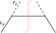
Figure 6.1: Lowest-order cut diagram describing the fragmentation of a quark into a pion.

As in the case of a pseudoscalar quark-pion coupling [34], the Collins function $H_{1}^{\perp}$ turns out to be zero in Born approximation. To obtain a nonzero result, we have to resort to the one-loop level. In Fig. 6.2 the corresponding diagrams are shown, where we have displayed only those graphs that contribute to the Collins function. The explicit calculation of $H_{1}^{\perp}$ is similar to our previous work [34]. The relevant ingredients of the calculation are the self-energy and the vertex correction diagrams. These ingredients are sketched in Fig. 6.3 and can be expressed analytically as

$$-{\rm i}\Sigma(k) =\frac{g_{A}^{2}}{4F_{\pi}^{2}}\int\frac{\operatorname{{\rm\,d}}^{4}l}{(2\pi)^{4}}\,\frac{\makebox[0.0pt][l]{$\sslash$}{l}\,(\makebox[0.0pt][l]{$\sslash$}{k}-\makebox[0.0pt][l]{$\sslash$}{l}-m)\,\makebox[0.0pt][l]{$\sslash$}{l}}{[(k-l)^{2}-m^{2}]\,[l^{2}-m_{\pi}^{2}]}\,,$$ (6.8a)

$$\Gamma_{1}(k,p) =-{\rm i}\frac{g_{A}^{3}}{8F_{\pi}^{3}}\,\gamma_{5}\int\frac{\operatorname{{\rm\,d}}^{4}l}{(2\pi)^{4}}\,\frac{\makebox[0.0pt][l]{$\sslash$}{l}\,(\makebox[0.0pt][l]{$\sslash$}{k}-\makebox[0.0pt][l]{\hskip 1.3pt$\sslash$}{p}-\makebox[0.0pt][l]{$\sslash$}{l}+m)}{[(k-p-l)^{2}-m^{2}]}\,\frac{\makebox[0.0pt][l]{\hskip 1.3pt$\sslash$}{p}\,(\makebox[0.0pt][l]{$\sslash$}{k}-\makebox[0.0pt][l]{$\sslash$}{l}-m)\,\makebox[0.0pt][l]{$\sslash$}{l}}{[(k-l)^{2}-m^{2}][l^{2}-m_{\pi}^{2}]}\,,$$ (6.8b)

$$\Gamma_{2}(k,p) =-{\rm i}\frac{g_{A}}{8F_{\pi}^{3}}\,\gamma_{5}\int\frac{\operatorname{{\rm\,d}}^{4}l}{(2\pi)^{4}}\,\frac{(\makebox[0.0pt][l]{$\sslash$}{l}+\makebox[0.0pt][l]{\hskip 1.3pt$\sslash$}{p})\,(\makebox[0.0pt][l]{$\sslash$}{l}-\makebox[0.0pt][l]{$\sslash$}{k}+m)\,\makebox[0.0pt][l]{$\sslash$}{l}}{[(k-l)^{2}-m^{2})][l^{2}-m_{\pi}^{2}]}\,,$$ (6.8c)

where flavor factors have been suppressed. For later purpose, we give here the most general parametrization of the functions $\Sigma$, $\Gamma_{1}$ and $\Gamma_{2}$,

$$\Sigma(k) =A\,\makebox[0.0pt][l]{$\sslash$}{k}+B\,m\,,\vphantom{\frac{1}{1}}$$ (6.9a)

$$\Gamma_{1}(k,p) =\frac{g_{A}}{2F_{\pi}}\,\gamma_{5}\,\Big{(}C_{1}+D_{1}\,\makebox[0.0pt][l]{\hskip 1.3pt$\sslash$}{p}+E_{1}\,\makebox[0.0pt][l]{$\sslash$}{k}+F_{1}\,\makebox[0.0pt][l]{\hskip 1.3pt$\sslash$}{p}\,\makebox[0.0pt][l]{$\sslash$}{k}\Big{)}\,,$$ (6.9b)

$$\Gamma_{2}(k,p) =\frac{g_{A}}{2F_{\pi}}\,\gamma_{5}\,\Big{(}C_{2}+D_{2}\,\makebox[0.0pt][l]{\hskip 1.3pt$\sslash$}{p}+E_{2}\,\makebox[0.0pt][l]{$\sslash$}{k}+F_{2}\,\makebox[0.0pt][l]{\hskip 1.3pt$\sslash$}{p}\,\makebox[0.0pt][l]{$\sslash$}{k}\Big{)}\,.$$ (6.9c)

The real parts of the functions $A$, $B$, $C_{1}$, $D_{1}$ etc. could be UV divergent and require in principle a proper renormalization. Here, we do not need to deal with the question of renormalization at all, since only the imaginary parts of the loop diagrams are important when calculating the Collins function [34].

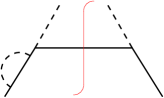
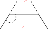
(a)                                (b)

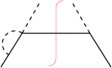
(c)

Figure 6.2: One-loop corrections to the fragmentation of a quark into a pion contributing to the Collins function. The Hermitean conjugate diagrams (h.c.) are not shown explicitly.

Figure 6.3: One-loop self-energy, and vertex corrections.

Taking now flavor factors properly into account, the contributions to the correlation function generated by the diagrams (a), (b) and (c) in Fig. 6.2 are given by

$$\Delta_{(1)}^{(a)}(k,p) =-3\,\frac{g_{A}^{2}}{4F_{\pi}^{2}}\,\frac{1}{(2\pi)^{4}}\,\frac{(\makebox[0.0pt][l]{$\sslash$}{k}+m)}{k^{2}-m^{2}}\,\gamma_{5}\,\makebox[0.0pt][l]{\hskip 1.3pt$\sslash$}{p}\,(\makebox[0.0pt][l]{$\sslash$}{k}-\makebox[0.0pt][l]{\hskip 1.3pt$\sslash$}{p}+m)\,$$

$$\quad\times\makebox[0.0pt][l]{\hskip 1.3pt$\sslash$}{p}\,\gamma_{5}\,\frac{(\makebox[0.0pt][l]{$\sslash$}{k}+m)}{k^{2}-m^{2}}\,\Sigma(k)\,\frac{(\makebox[0.0pt][l]{$\sslash$}{k}+m)}{k^{2}-m^{2}}\,2\pi\,\delta\left((k-p)^{2}-m^{2}\right)\,,\vphantom{\frac{1}{1}}$$ (6.10a)

$$\Delta_{(1)}^{(b)}(k,p) =\frac{g_{A}}{2F_{\pi}^{2}}\,\frac{1}{(2\pi)^{4}}\,\frac{(\makebox[0.0pt][l]{$\sslash$}{k}+m)}{k^{2}-m^{2}}\,\gamma_{5}\,\makebox[0.0pt][l]{\hskip 1.3pt$\sslash$}{p}\,(\makebox[0.0pt][l]{$\sslash$}{k}-\makebox[0.0pt][l]{\hskip 1.3pt$\sslash$}{p}+m)$$

$$\quad\times\Gamma_{1}(k,p)\,\frac{(\makebox[0.0pt][l]{$\sslash$}{k}+m)}{k^{2}-m^{2}}\,2\pi\,\delta\left((k-p)^{2}-m^{2}\right)\,,$$ (6.10b)

$$\Delta_{(1)}^{(c)}(k,p) =-2\frac{g_{A}}{2F_{\pi}^{2}}\,\frac{1}{(2\pi)^{4}}\,\frac{(\makebox[0.0pt][l]{$\sslash$}{k}+m)}{k^{2}-m^{2}}\,\gamma_{5}\,\makebox[0.0pt][l]{\hskip 1.3pt$\sslash$}{p}\,(\makebox[0.0pt][l]{$\sslash$}{k}-\makebox[0.0pt][l]{\hskip 1.3pt$\sslash$}{p}+m)$$

$$\quad\times\Gamma_{2}(k,p)\,\frac{(\makebox[0.0pt][l]{$\sslash$}{k}+m)}{k^{2}-m^{2}}\,2\pi\,\delta\left((k-p)^{2}-m^{2}\right)\,.$$ (6.10c)

The correlation functions of the Hermitean conjugate diagrams follow from the Hermiticity condition $\Delta_{(1)}^{H.c.}(k,p)=\gamma^{0}\Delta_{(1)}^{\dagger}(k,p)\,\gamma^{0}$.

Summing the contributions of all diagrams and inserting the resulting correlation function in Eq. (6.1b), we eventually obtain the result

$$H_{1}^{\perp}(z,z^{2}\bm{k}^{2}_{T})=\frac{g_{A}^{2}}{32\pi^{3}F_{\pi}^{2}}\,\frac{m_{\pi}}{1-z}\,\frac{1}{k^{2}-m^{2}}\,\bigg{(}-3m\operatorname{\,{\rm Im}\,}\big{(}A+B\big{)}-\operatorname{\,{\rm Im}\,}\big{(}C_{1}-mE_{1}+(k^{2}-m^{2})F_{1}\big{)}\\ +2\operatorname{\,{\rm Im}\,}\big{(}C_{2}-mE_{2}+(k^{2}-m^{2})F_{2}\big{)}\bigg{)}\,\bigg{|}_{k^{2}=\frac{z}{1-z}k_{T}^{2}+\frac{m^{2}}{1-z}+\frac{m_{\pi}^{2}}{z}}\,.$$ (6.11)

Thus, the Collins function is entirely given by the imaginary parts of the coefficients defined in Eqs. (6.9). We can compute these imaginary parts by applying Cutkosky rules to the self-energy and vertex diagrams of Fig. 6.3. Explicit calculation leads to

$$\operatorname{\,{\rm Im}\,}\big{(}A+B\big{)} =\frac{g_{A}^{2}}{32\pi^{2}F_{\pi}^{2}}\,\bigg{(}2m_{\pi}^{2}-\frac{k^{2}-m^{2}}{2}\,\Big{(}1-\frac{m^{2}-m_{\pi}^{2}}{k^{2}}\Big{)}\bigg{)}\,I_{1}\,,$$ (6.12a)

$$\operatorname{\,{\rm Im}\,}\big{(}C_{1}-mE_{1}+(k^{2}-m^{2})F_{1}\big{)} =\frac{g_{A}^{2}}{32\pi^{2}F_{\pi}^{2}}\,m\,(k^{2}-m^{2})\,\bigg{(}\frac{3k^{2}+m^{2}-m_{\pi}^{2}}{2k^{2}}\,I_{1}$$ (6.12b)

$$\quad+4m^{2}\,\frac{k^{2}-m^{2}+m_{\pi}^{2}}{\lambda(k^{2},m^{2},m_{\pi}^{2})}\,\Big{(}I_{1}+(k^{2}-m^{2}-2m_{\pi}^{2})\,I_{2}\Big{)}\bigg{)}\,,$$

$$\operatorname{\,{\rm Im}\,}\big{(}C_{2}-mE_{2}+(k^{2}-m^{2})F_{2}\big{)} =\frac{1}{32\pi^{2}F_{\pi}^{2}}\,m\,(k^{2}-m^{2})\,\bigg{(}1-\frac{m^{2}-m_{\pi}^{2}}{k^{2}}\bigg{)}\,I_{1}\,,$$ (6.12c)

where we have introduced the so-called Källen function, $\lambda(k^{2},m^{2},m_{\pi}^{2})=[k^{2}-(m+m_{\pi})^{2}][k^{2}-(m-m_{\pi})^{2}]$, and the factors

$$I_{1} =\int\operatorname{{\rm\,d}}^{4}l\;\delta\left(l^{2}-m_{\pi}^{2}\right)\,\delta\left((k-l)^{2}-m^{2}\right)=\frac{\pi}{2k^{2}}\,\sqrt{\lambda(k^{2},m^{2},m_{\pi}^{2})}\;\theta\left(k^{2}-(m+m_{\pi})^{2}\right)\,,$$ (6.13a)

$$I_{2} =\int\operatorname{{\rm\,d}}^{4}l\;\frac{\delta\left(l^{2}-m_{\pi}^{2}\right)\,\delta\left((k-l)^{2}-m^{2}\right)}{(k-p-l)^{2}-m^{2}}$$

$$=-\frac{\pi}{2\sqrt{\lambda(k^{2},m^{2},m_{\pi}^{2})}}\,\ln{\left|1+\frac{\lambda(k^{2},m^{2},m_{\pi}^{2})}{k^{2}m^{2}-(m^{2}-m_{\pi}^{2})^{2}}\right|}\;\theta\left(k^{2}-(m+m_{\pi})^{2}\right)\,.$$ (6.13b)

These integrals are finite and vanish below the threshold of quark-pion production, where the self-energy and vertex diagrams do not possess an imaginary part.

Thus, Eq. (6.11) in combination with Eqs. (6.12) gives the explicit result for the Collins function in the Manohar-Georgi model to lowest possible order. Because of its chiral-odd nature, the Collins function would vanish in this model if we set the mass of the quark to zero. The same phenomenon has been observed in the calculation of a chiral-odd twist-3 fragmentation function [121]. The result in Eq. (6.11) corresponds, e.g., to the fragmentation $u\to\pi^{0}$. The expressions for the remaining favored transitions are obtained in analogy to Eqs. (6.7). Unfavored fragmentation processes in the case of the Collins function appear only at the two-loop level.

6.2 Estimates and phenomenology

6.2.1 Unpolarized fragmentation function and the choice of parameters

We now present our numerical estimates, where all results for the fragmentation functions in this subsection refer to the transition $u\to\pi^{+}$. To begin with we calculate the unpolarized fragmentation function $D_{1}(z)$, which is given by

$$D_{1}(z)=\pi\int_{0}^{K^{2}_{T\,{\rm max}}}\operatorname{{\rm\,d}}\bm{K}^{2}_{T}\;D_{1}(z,\bm{K}^{2}_{T}),$$ (6.14)

where $\bm{K}_{T}=-z\bm{k}_{T}$ denotes the transverse momentum of the outgoing hadron with respect to the quark direction. The upper limit on the $\bm{K}^{2}_{T}$ integration is set by the cutoff on the fragmenting quark virtuality, $\mu^{2}$, and corresponds to

$$K^{2}_{T\,{\rm max}}=z\,(1-z)\,\mu^{2}-z\,m^{2}-(1-z)\,m_{\pi}^{2}\,.$$ (6.15)

In addition to $m$ and $g_{A}$, the cutoff $\mu^{2}$ is the third parameter of our approach that is not fixed a priori. However, as will be explained below, the possible values of $\mu^{2}$ can be restricted when comparing our results to experimental data. Unless otherwise specified, we always use the values

$$m=0.3\;{\rm GeV},\qquad g_{A}=1,\qquad\mu^{2}=1\;{\rm GeV}^{2}\,.$$ (6.16)

At the relevant places, the dependence of our results on possible variations of these parameters will be discussed. A few remarks concerning the choice in Eq. (6.16) are in order. The value of $m$ is a typical mass of a constituent quark. The choice for the axial coupling can be seen as a kind of average number of what has been proposed in the literature. For instance, in a simple SU(6) spin-flavor model for the proton one finds $g_{A}\approx 0.75$ in order to obtain the correct value for the axial charge of the nucleon [139]. On the other hand, large $N_{c}$ arguments favor a value of the order of 1 [171], while, according to a recent calculation in a relativistic point-form approach [59], a $g_{A}$ slightly above 1 seems to be required for describing the axial charge of the nucleon. Finally, our choice for $\mu^{2}$ ensures that the momenta of the outgoing pion and quark, in the rest frame of the fragmenting quark, remain below values of the order $0.5\,\rm{GeV}$. In this region we believe chiral perturbation theory to be applicable, meaning that our leading order result can provide a reliable estimate.

In Fig. 6.4 we show the result for the unpolarized fragmentation function $D_{1}^{u\rightarrow\pi^{+}}$. Notice that in general the fragmentation functions vanish outside the kinematical limits, which in our model are given by

$$z_{{\rm max},{\rm min}}=\frac{1}{2}\left[\left(1-\frac{m^{2}-m_{\pi}^{2}}{\mu^{2}}\right)\pm\sqrt{\left(1-\frac{m^{2}-m_{\pi}^{2}}{\mu^{2}}\right)^{2}-4\,\frac{m_{\pi}^{2}}{\mu^{2}}}\right],$$ (6.17)

corresponding to the situation when the upper limit of the $K_{T}^{2}$ integration becomes equal to zero. We consider our tree level result as a pure valence-type part of $D_{1}^{u\rightarrow\pi^{+}}$. The sea-type (unfavored) transition $\bar{u}\to\pi^{+}$ is strictly zero at leading order. Therefore, we compare the model result to the valence-type quantity $D_{1}^{u\rightarrow\pi^{+}}-D_{1}^{\bar{u}\rightarrow\pi^{+}}$, where the fragmentation functions have been taken from the parametrization of Kretzer [129] at a scale $Q^{2}=1\,\rm{GeV}^{2}$. Obviously, the $z$ dependence of both curves is in nice agreement, which is a nontrivial result. For example, in the pseudoscalar model that we used in our previous work [34], $D_{1}$ behaves quite differently and peaks at an intermediate $z$ value.

On the other hand, we underestimate the parametrization of Ref. 129 by about a factor of 2. Some remarks are in order at this point. Although a part of the discrepancy might be attributed to the uncertainty in the value of $g_{A}$, the most important point is to address the question as to what extent we can compare our estimate with existing parametrizations. The parametrization of [129] serves basically as input function of the perturbative QCD evolution equations, used to describe high-energy $e^{+}e^{-}$ data, and displays the typical logarithmic dependence on the scale $Q^{2}$. A value of $Q^{2}=1$ GeV² is believed to be already beyond the limit of applicability of perturbative QCD calculations. On the other hand, our approach displays, to a first approximation, a linear dependence on the cutoff $\mu^{2}$. It is supposed to be valid at low scales and it is also stretched to the limit of its applicability for $\mu^{2}=1$ GeV². In this context it should also be investigated to what extent the inclusion of one-loop corrections, which allow for the additional decay channel $q^{\ast}\to\pi\pi q$, will increase the result for $D_{1}$ at $\mu^{2}=1\,\rm{GeV}^{2}$. Finally, we want to remark that to our knowledge there exists no strict one-to-one correspondence between the quark virtuality $\mu^{2}$ and the scale used in the evolution equation of fragmentation functions, which in semi-inclusive DIS is typically identified with the photon virtuality $Q^{2}$. For all these reasons, a smooth matching of our calculation and the parametrization of [129] cannot necessarily be expected. Despite these caveats, the correct $z$ behavior displayed by our result for $D_{1}$ suggests that the calculation can well be used as an input for evolution equations at a low scale. In the next subsection we will elaborate more on this point in connection with the Collins function.

Figure 6.4: Model result for the unpolarized quark fragmentation function $D_{1}^{u\rightarrow\pi^{+}}$ (solid line) and comparison with the parametrization of Ref. [129] (gray line).

Figure 6.5: Model result for the average hadron transverse momentum for different choices of the cutoff: $\mu^{2}=0.5$ GeV² (dotted line), $\mu^{2}=1$ GeV² (solid line), $\mu^{2}=1.5$ GeV² (dashed line) and comparison with a fit to experimental results from DELPHI [3] (gray line).

The best indication of the appropriate value of the cutoff $\mu^{2}$ may be obtained when comparing our calculation to experimental data of the average transverse momentum of the outgoing hadron with respect to the quark, which we evaluate according to

$$\langle|\bm{K}_{T}|(z)\rangle=\frac{\pi}{D_{1}(z)}\int_{0}^{K^{2}_{T\,{\rm max}}}\operatorname{{\rm\,d}}\bm{K}^{2}_{T}\,|\bm{K}_{T}|\,D_{1}(z,\bm{K}^{2}_{T})\,.$$ (6.18)

In Fig. 6.5 we show the result of this observable as a function of $z$ for three different choices of the parameter $\mu^{2}$. As a comparison, we also show a fit (taken from Ref. 23) to experimental data obtained by the DELPHI Collaboration [3]. As in the case of $D_{1}(z)$, the shape of our result is very similar to the experimental one, which we consider as an encouraging result. For $\mu^{2}=1\,\rm{GeV}^{2}$ our curve is about $30\%$ below the data. Such a disagreement is not surprising, keeping in mind that at LEP energies higher order perturbative QCD effects (e.g. gluon bremsstrahlung, unfavored fragmentations, etc.) play an important role, leading in general to a broadening of the $\bm{K}_{T}$ distribution. For experiments at lower energies, however, where perturbative QCD contributions can be neglected in a first approximation, it may be possible to exhaust the experimental value for $\langle|\bm{K}_{T}|(z)\rangle$ with genuine soft contributions as described in our model. This in turn would determine the appropriate value of the cutoff $\mu^{2}$. For example, such a method of matching our calculation with experimental conditions could be applied at HERMES kinematics, even though the method is somewhat hampered since $\bm{K}_{T}$ is not directly measured in semi-inclusive DIS. In this case, one rather observes the transverse momentum of the outgoing hadron with respect to the virtual photon, $\bm{P}_{h\perp}$, which depends on both $\bm{K}_{T}$ and the transverse momentum of the partons inside the target $\bm{p}_{T}$, as shown in Eq. (3.40).

6.2.2 Collins function

We now turn to the description of our model result for the Collins function. In Fig. 6.6, $H_{1}^{\perp}$ is plotted for three different values of the constituent quark mass, $m=0.2,\,0.3,\,0.4$ GeV. In a large $z$ range, the function does not depend strongly on the precise value of the quark mass, if we choose it within reasonable limits. That is why we can confidently fix $m=0.3\,\rm{GeV}$ for our numerical studies. It is very interesting to observe that the behavior of the unpolarized fragmentation function $D_{1}$ is quite distinct from that of the Collins function: while the former is decreasing as $z$ increases, the latter is growing.

Figure 6.6: Model result for the Collins function for different values of the constituent quark mass: $m=0.2$ GeV (dotted line), $m=0.3$ GeV (solid line), $m=0.4$ GeV (dashed line).

The different behavior of the two functions becomes even more evident when looking at their ratio, shown in Fig. 6.7. At present, there exists some evidence of $z$ behavior of the Collins function and it is in agreement with our results. We briefly discuss this subject in Sec. 6.3.

The ratios of the Collins function or any of its moments with $D_{1}$ are almost independent of the coupling constant $g_{A}$. The reason is that the one-loop correction containing the contact interaction is only proportional to $g_{A}^{2}$, as $D_{1}$ is, and is dominating over the others. Furthermore, the ratio $H_{1}^{\perp}/D_{1}$ is nearly independent of the cutoff $\mu^{2}$. In conclusion, the prediction shown in Fig. 6.7 is almost independent of the choice of parameters in our approach.

Figure 6.7: Model result for $H_{1}^{\perp}/D_{1}$.

At this point we would like to add some general remarks concerning the $z$ behavior of our results. It turns out that the shape of all the results does not vary much when changing the parameters within reasonable limits. In particular, variations of $g_{A}$ and of the cutoff $\mu^{2}$ only change the normalization of the curves but not their shape. In this sense our calculation of fragmentation functions has a good predictive power for the $z$ behavior of the function. This has a direct practical consequence if one uses, for instance, our result of the Collins function as input in an evolution equation: the $z$ dependence of the input function can be adjusted to the shape of our $H_{1}^{\perp}$, while its normalization can be kept free in order to account for uncertainties in the values of $g_{A}$ and $\mu^{2}$.

In Fig. 6.8 we plot the ratio

$$\frac{H_{1}^{\perp(1/2)}(z)}{D_{1}(z)}\equiv\frac{\pi}{D_{1}(z)}\int\operatorname{{\rm\,d}}K_{T}^{2}\,\frac{|\bm{K}_{T}|}{2zm_{\pi}}\,H_{1}^{\perp}(z,K_{T}^{2})\,,$$ (6.19)

which enters the transverse single spin asymmetry of Eq. (3.43). This quantity rises roughly linearly within a large $z$ range, leading to a similar $z$ behavior of the transverse spin asymmetry. $H_{1}^{\perp(1/2)}/D_{1}$ is no longer independent of the cutoff $\mu^{2}$, but rather the same dependence as in the case of $\langle|\bm{K}_{T}|\rangle$ (Fig. 6.5) can be assumed. In Fig. 6.8, this ratio is compared to the expression

$$\frac{\langle|\bm{K}_{T}|(z)\rangle}{2zm_{\pi}}\,\frac{H_{1}^{\perp}(z)}{D_{1}(z)}=\pi\,\frac{H_{1}^{\perp}(z)}{D_{1}^{2}(z)}\int\operatorname{{\rm\,d}}K_{T}^{2}\,\frac{|\bm{K}_{T}|}{2zm_{\pi}}\,D_{1}(z,K_{T}^{2})\,.$$ (6.20)

A very close agreement between the two different curves can be observed, indicating that the model predicts a quite similar transverse momentum dependence of both the Collins function and $D_{1}$. In the literature, this feature is sometimes assumed in phenomenological parametrizations of $H_{1}^{\perp}$. Note, however, that in our approach deviations from this simple behavior can be expected, if $D_{1}$ is also calculated consistently to the one-loop order.

Figure 6.8: Model result for $H_{1}^{\perp(1/2)}/D_{1}$ (solid line) and comparison with the product $(\langle|\bm{K}_{T}|\rangle/2zm_{\pi})\,(H_{1}^{\perp}/D_{1})$ (dashed line). Note that the positivity bound requires the ratio to be smaller than $0.5$.

The Collins function has to fulfill the positivity bound of Eq. (3.33b), which can be rewritten as

$$\frac{|\bm{K}_{T}|}{2zm_{\pi}}\,H_{1}^{\perp}(z,K_{T}^{2})\leq\frac{1}{2}\,D_{1}(z,K_{T}^{2}).$$ (6.21)

Integration over $K_{T}^{2}$ gives the simplified expression

$$\frac{H_{1}^{\perp(1/2)}(z)}{D_{1}(z)}\leq\frac{1}{2}\,,$$ (6.22)

which is satisfied by our model calculation. It is clear, however, that increasing the value of $\mu^{2}$ will eventually result in a violation of the positivity condition. To avoid such a violation, we should calculate $D_{1}$ and $H_{1}^{\perp}$ consistently at the same order, i.e., the one-loop corrections to $D_{1}$ should be included. By doing so, the positivity bound will be fulfilled even at larger values of $\mu^{2}$, for which our numerical results are no longer trustworthy.

From our results, we expect an increasing behavior of the azimuthal asymmetry in $p^{\uparrow}p\to\pi\,X$ as function of $x_{F}$, qualitatively similar to what has been predicted in Ref. 26 in the context of the Lund fragmentation model. At this point, it is also interesting to discuss the comparison of our results with the ones obtained using the so-called “Collins guess”. On the basis of very general assumptions, Collins suggested a possible behavior for the transverse spin asymmetry containing $H_{1}^{\perp}$ [77]. This suggestion has been used in the literature (see, e.g., Refs. 145, 128, 87, 137) to propose the following shape for the Collins function:

$$H_{1}^{\perp(1/2)}(z)\approx\pi\int\operatorname{{\rm\,d}}K_{T}^{2}\,\frac{|\bm{K}_{T}|}{2z}\,\frac{M_{C}}{M_{C}^{2}+{K_{T}^{2}/z^{2}}}\,D_{1}(z,K_{T}^{2}),$$ (6.23)

with the parameter $M_{C}$ ranging between 0.3 and $0.7\,\rm{GeV}$. Using our model outcome for the unpolarized fragmentation function, we apply Eq. (6.23) to estimate $H_{1}^{\perp(1/2)}$, and in Fig. 6.9 we show how this compares to Eq. (6.19). There is a rough qualitative agreement with the Collins ansatz for the lowest value of the parameter $M_{C}$, although it is not growing fast enough compared to Eq. (6.19). On the other hand, in the Manohar-Georgi model there is no agreement with the Collins ansatz for high values of the parameter $M_{C}$, which might indicate that the relation suggested in Eq. (6.23) should be handled with care.

Figure 6.9: Model result for $H_{1}^{\perp(1/2)}/D_{1}$ (solid line) and comparison with the same ratio, where $H_{1}^{\perp(1/2)}$ is calculated according to Eq. (6.23) with $M_{C}=0.3$ GeV (dashed line) and $M_{C}=0.7$ GeV (dotted line).

Finally, in Fig. 6.10 we display the quantity

$$\frac{H_{1}^{\perp(1)}(z)}{D_{1}(z)}\equiv\frac{\pi}{D_{1}(z)}\int\operatorname{{\rm\,d}}K_{T}^{2}\,\frac{K_{T}^{2}}{2z^{2}m_{\pi}^{2}}\,H_{1}^{\perp}(z,K_{T}^{2})\,,$$ (6.24)

because this ratio appears in the weighted asymmetries of Eq. (3.48). In Fig. 6.10, the expression

$$\frac{\langle K_{T}^{2}\rangle(z)}{2z^{2}m_{\pi}^{2}}\frac{H_{1}^{\perp}(z)}{D_{1}(z)}=\pi\,\frac{H_{1}^{\perp}(z)}{D_{1}^{2}(z)}\int\operatorname{{\rm\,d}}K_{T}^{2}\frac{K_{T}^{2}}{2z^{2}m_{\pi}^{2}}D_{1}(z,K_{T}^{2})\,$$ (6.25)

is also shown for comparison. Once again, there is a remarkable agreement between the two different expressions, confirming the quite similar $K_{T}$ behavior of $H_{1}^{\perp}$ and $D_{1}$.

Figure 6.10: Model result $H_{1}^{\perp(1)}/D_{1}$ (solid line) and comparison with the product $(\langle K_{T}^{2}\rangle/2z^{2}m_{\pi}^{2})(H_{1}^{\perp}/D_{1}^{\perp})$ (dashed line).

6.2.3 Asymmetries in semi-inclusive DIS and $e^{+}e^{-}$ annihilation

We turn now to estimates of possible observables containing the Collins function. We will take into consideration one-particle inclusive DIS, where the Collins function appears in connection with the transversity distribution of the nucleon, and $e^{+}e^{-}$ annihilation into two hadrons belonging to two different jets.

In the first case, we show predictions for both transverse spin asymmetries defined in Eqs. (3.43) and (3.48). Different calculations can be found in the literature, e.g., in Refs. 22, 126, 137. To estimate the magnitude of the asymmetries, we need inputs for the distribution functions, in particular for the transversity distribution. Several model calculations of this function are available at present (see [41] for a comprehensive review). We refrain from considering many different examples and rather restrict the analysis to two limiting situations. In the first case we adopt the “nonrelativistic” assumption $h_{1}=g_{1}$, while in the second case we exhaust the upper bound on the transversity distribution, i.e., $h_{1}=\frac{1}{2}(f_{1}+g_{1})$ [159]. We use the simple parametrization of $g_{1}$ and $f_{1}$ suggested in Ref. 70. At the moment, more sophisticated parametrizations are available, taking scale evolution into account also. However, all these parametrizations are compatible with each other to the extent of our purpose here, which is to give an estimate of the asymmetries for a low scale. We focus on the production of $\pi^{+}$, where the contribution of down quarks is negligible, not only because of the presence of unfavored fragmentation functions, but also because the transversity distribution for down quarks appears to be much smaller than for up quarks in model calculations.

In Fig. 6.11 we present the azimuthal asymmetry defined in Eq. (3.43) as a function of $x_{B}$, after integrating numerator and denominator over the variables $y$ and $z_{h}$, for the two cases described above. In Fig. 6.12, we present the same asymmetry as a function of $z_{h}$, after integrating over $y$ and $x_{B}$. As already mentioned before, our prediction is supposed to be valid at a low energy scale of about $1\,\rm{GeV}^{2}$. Neglecting evolution effects, it could be utilized for comparison with experiments at a scale of a few GeV². We assume the value of the transverse polarization to be $|\bm{S}_{T}|=0.75$. In performing the integrations, we apply the kinematical cuts typical of the HERMES experiment, as described in [10]. Therefore, our prediction is particularly significant for HERMES, which is expected to be the first experiment to measure this asymmetry. In principle, the simultaneous study of the $x_{B}$ and $z_{h}$ dependence of the asymmetry yields separate information on the distribution and fragmentation parts and allows one to extract both up to a normalization factor [126]. Note, however, that this procedure relies on the assumption of up-quark dominance and is valid only if the $x_{B}$ dependence of the asymmetry can be ascribed entirely to the distribution functions and the $z_{h}$ dependence entirely to the fragmentation functions. Kinematical cuts could partially spoil this situation. We would like to stress that our calculation predicts an asymmetry up to the order of 10%, which should be within experimental reach, and suggests the possibility of distinguishing between different assumptions on the transversity distribution.

Figure 6.11: Azimuthal transverse spin asymmetry $\langle\sin{\phi}\rangle_{UT}$ as a function of $x_{B}$. Solid line: assuming $h_{1}=g_{1}$. Dashed line: assuming $h_{1}=\frac{1}{2}(f_{1}+g_{1})$. The functions $f_{1}$ and $g_{1}$ are taken from [70].

Figure 6.12: Azimuthal transverse spin asymmetry $\langle\sin{\phi}\rangle_{UT}$ as a function of $z_{h}$. Solid line: assuming $h_{1}=g_{1}$. Dashed line: assuming $h_{1}=\frac{1}{2}(f_{1}+g_{1})$. The functions $f_{1}$ and $g_{1}$ are taken from [70].

Using the same procedure as before, we have estimated the asymmetry defined in Eq. (3.48), containing the weighting with $|\bm{P}_{h\perp}|/m_{\pi}$. The results are shown in Fig. 6.13 as a function of $x_{B}$ and in Fig. 6.14 as a function of $z_{h}$. The magnitude of this asymmetry is higher than in the unweighted case, which is partially due to the fact that the weighting enhances the asymmetry by about a factor of 2.

Figure 6.13: Azimuthal spin asymmetry $\langle|\bm{P}_{h\perp}|/m_{\pi}\,\sin{\phi}\rangle_{UT}$ as a function of $x_{B}$. Solid line: assuming $h_{1}=g_{1}$. Dashed line: assuming $h_{1}=\frac{1}{2}(f_{1}+g_{1})$. The functions $f_{1}$ and $g_{1}$ are taken from [70].

Figure 6.14: Azimuthal spin asymmetry $\langle|\bm{P}_{h\perp}|/m_{\pi}\,\sin{\phi}\rangle_{UT}$ as a function of $z_{h}$. Solid line: assuming $h_{1}=g_{1}$. Dashed line: assuming $h_{1}=\frac{1}{2}(f_{1}+g_{1})$. The functions $f_{1}$ and $g_{1}$ are taken from [70].

In addition to appearing in semi-inclusive DIS in connection with the transversity distribution of the nucleon, the Collins function can be independently extracted from another process, i.e. electron-positron annihilation into two hadrons belonging to two back-to-back jets [51, 52]. We restrict ourselves to the case of photon exchange only. In this process, one of the two hadrons (say hadron 2) defines the scattering plane together with the leptons and determines the direction with respect to which the azimuthal angles must be measured. The cross section is differential in five variables, e.g. $z_{1},z_{2},y,|\bm{P}_{h\perp}|,\phi$. The variables $z_{1}$ and $z_{2}$ are the longitudinal fractional momenta of the two hadrons. In the center of mass frame $y=(1+\cos{\theta})/2$, where $\theta$ is the angle of hadron 2 with respect to the momentum of the incoming leptons. The vector $\bm{P}_{h\perp}$ denotes the transverse component of the momentum of hadron 1 and $\phi$ is its azimuthal angle with respect to the scattering plane. For a more detailed description of the kinematical variables we refer to [51, 52].

We define the azimuthal asymmetry

$$\begin{split}\left\langle P_{h\perp}^{2}\cos{2\phi}\right\rangle_{e^{+}e^{-}}(\theta,z_{1},z_{2})&=\frac{\int\operatorname{{\rm\,d}}^{2}\bm{P}_{h\perp}\,\lvert\bm{P}_{h\perp}\rvert^{2}\,\cos{2\phi}\;\operatorname{{\rm\,d}}^{5}\sigma_{e^{+}e^{-}}}{\int\operatorname{{\rm\,d}}^{2}\bm{P}_{h\perp}\,\lvert\bm{P}_{h\perp}\rvert^{2}\,\operatorname{{\rm\,d}}^{5}\sigma_{e^{+}e^{-}}}\\ &=\frac{2\,\sin^{2}{\theta}}{1+\cos^{2}{\theta}}\,\frac{H_{1}^{\perp(1)}(z_{1})\,\bar{H}_{1}^{\perp(1)}(z_{2})}{\left(D_{1}(z_{1})\,\bar{D}_{1}^{(1)}(z_{2})+D_{1}^{(1)}(z_{1})\,\bar{D}_{1}(z_{2})\right)},\end{split}$$ (6.26)

where summations over quark flavors are understood. The weighting with a second power of $\lvert\bm{P}_{h\perp}\rvert$ in the numerator is necessary to obtain a deconvoluted expression. We prefer to use the same weighting in the denominator as well, to avoid a modification of the asymmetry just caused by the weighting.

In Fig. 6.15 we present the estimate of the asymmetry defined above, entirely based on our model. The asymmetry has been integrated over $z_{2}$ and $\theta$, leaving the dependence on $z_{1}$ alone. We have extended the $\theta$ integration interval all the way to $[0,\pi]$, to obtain a conservative estimate. In fact, limiting the interval to $[{\pi/4},{3\pi/4}]$ will enhance the asymmetry by a factor of 2, approximately. Because the Collins function increases with increasing $z$, we also get a larger asymmetry by restricting the integration range for $z_{2}$. As an illustration of this feature, in Fig. 6.15 we present two results, obtained from two different integration ranges. Our prediction is supposed to be valid only at low energy scales and should be evolved for comparison with higher energy experiments. It is important to note that we estimate the asymmetry to be of the order of about 5%, and thus it should observable in experiments.

Figure 6.15: Azimuthal asymmetry $\langle P_{h\perp}^{2}\cos{2\phi}\rangle_{e^{+}e^{-}}$ for $e^{+}e^{-}$ annihilation into two hadrons, integrated over the range $0.2\leq z_{2}\leq 0.8$ (solid line), and over the range $0.5\leq z_{2}\leq 0.8$ (dashed line).

6.3 Comparison with existing data

The HERMES collaboration recently measured the single longitudinal spin asymmetry

$$\langle\sin\phi_{h}\rangle_{UL}\propto\frac{1}{Q}\Big{[}\Big{(}c_{1}\,h_{L}(x)+c_{2}\,h_{1}(x)\Big{)}H_{1}^{\perp(1/2)}(z)\,+\,\text{other terms}\Big{]}.$$ (6.27)

On purpose, we avoid entering the details of the formula. It is difficult to extract information on the Collins function and on the transversity distribution from this asymmetry [61]. In a recent analysis of this asymmetry, Efremov et al. [90] extracted a behavior $H_{1}^{\perp}/D_{1}\propto z$ for $z\leq 0.7$, although some questionable assumptions were used to obtain this result.

If we assume that the other terms in (6.27) are small, then the $z_{h}$ dependence of the asymmetry should be almost entirely due to the Collins function. To compare this behavior with our model estimate, as a first step we parametrize our result for the ratio $H_{1}^{\perp(1/2)}/D_{1}$ with a simple analytic form

$$\frac{H_{1}^{\perp(1/2)}(z)}{D_{1}(z)}\approx 0.316\,z+0.0345\,\frac{1}{1-z}-0.00359\,\frac{1}{(1-z)^{2}}.$$ (6.28)

Fig. 6.16 shows the result of our model together with this parametrization (note that we extended the plot to higher values of $z$ compared to Fig. 6.8).

Figure 6.16: Model result for the ratio $H_{1}^{\perp(1/2)}/D_{1}$ as a function of $z$ and the simple analytic parametrization of Eq. (6.28).

In Fig. 6.17 we compare our parametrization with HERMES data on $\langle\sin\phi_{h}\rangle_{UL}$ [11] and preliminary data on the same asymmetry from the CLAS collaboration at JLAB [30]. Note that we arbitrarily normalized our curve to take into account the unknown distribution functions and prefactors. The agreement of the $z_{h}$ shape is remarkable.

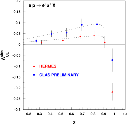
Figure 6.17: Comparison between the results of our model and data from the HERMES and CLAS experiments.

6.4 Summary

We have estimated the Collins fragmentation function for pions at a low energy scale by means of the Manohar-Georgi model. This model contains three essential features of nonperturbative QCD: massive quark degrees of freedom, chiral symmetry and its spontaneous breaking (with pions as Goldstone bosons). Because of the chiral invariant interaction between pions and quarks, the fragmentation process can be evaluated in a perturbative expansion. The constituent quark mass, the axial pion-quark coupling $g_{A}$ and the maximum virtuality $\mu^{2}$ of the fragmenting quark are free parameters of our approach. The quark mass and $g_{A}$ are constrained within reasonable limits. To ensure the convergence of the chiral perturbation expansion, $\mu^{2}$ cannot exceed a typical hadronic scale. We have mostly considered the value $\mu^{2}=1\,\rm{GeV}^{2}$, which guarantees that the momenta of the particles produced in the fragmentation process stay well below the scale of chiral symmetry breaking, $\Lambda_{\chi}\approx 1$ GeV. To determine the appropriate value of $\mu^{2}$, the average transverse momentum of a data set could be used. In any case, we observed that variations of the free parameters within reasonable limits have only a minor influence on the shape of the results, implying that our approach has a good predictive power for the $z$ behavior of the various functions.

We have found that the Manohar-Georgi model reproduces reasonably well the unpolarized pion fragmentation function and the average transverse momentum of a produced hadron as a function of $z$, supporting the idea of describing the fragmentation process by such a chiral invariant approach.

Compared to the unpolarized fragmentation function, modeling the Collins function is considerably more difficult, mainly because of its chiral-odd and T-odd nature. In our approach, the helicity flip required to generate a chiral-odd object is caused by the mass of the constituent quark, while the T-odd behavior is produced via one-loop corrections. The Collins function exhibits a quite distinct behavior from the unpolarized fragmentation function. In particular, the ratio $H_{1}^{\perp}/D_{1}$ is strongly increasing with increasing $z$.

On the basis of our results, we have calculated the transverse single-spin asymmetry in semi-inclusive DIS where the Collins function appears in combination with the transversity of the nucleon. This observable will be measured in the near future at HERMES and could also be investigated at COMPASS, Jlab (upgraded) and EIC. For typical HERMES kinematics the asymmetry is of the order of $10\%$, giving support to the intention of extracting the nucleon transversity in this way. We believe that our estimate of the Collins function, despite its uncertainties, can be very useful for this extraction. Finally, we found an encouraging agreement between the shape of our estimate and the trend of the single spin asymmetry measured by the HERMES collaboration [10, 11], although it is not clear if this asymmetry is originated solely by the Collins function.

More information on the Collins function from the experimental side is required. In this respect, the most promising experiment seems to be $e^{+}e^{-}$ annihilation into two hadrons, where $H_{1}^{\perp}$ appears squared in an azimuthal $\cos{2\phi}$ asymmetry. According to our calculation, an asymmetry of the order of $5\%$ can be expected, which should be measurable at high luminosity accelerators, such as BABAR and BELLE [146]. Dedicated measurements of the Collins function would be extremely important for the extraction of the transversity distribution. Moreover, they could answer the question whether a chiral invariant Lagrangian can be used to model the Collins function.

Chapter 7 Conclusions and outlook

The main focus of this thesis was to present some ways of accessing the transversity distribution of quarks inside hadrons, $h_{1}$. This was the main motivation to perform a thorough analysis of one-particle and two-particle inclusive deep inelastic scattering at leading order in $1/Q$, with a particular attention to T-odd fragmentation functions. This thesis is certainly not the first work on this important subject, however it complements the existing literature in many respects.

7.1 Conclusions

Several observables containing the transversity distribution appear all along the thesis, but three of them are particularly promising and have been highlighted. The first method presented to access transversity is the measurement of the azimuthal single spin asymmetry described in Eq. (3.48), or the similar asymmetry described in Eq. (3.43). In these asymmetries, the transversity distribution appears in combination with the Collins fragmentation function, which provides the chirality flip necessary to compensate the chiral-odd nature of $h_{1}$.

The Collins function was introduced in Ref. 77 as early as 1993. However, it was looked at with some skepticism because it is a single-particle T-odd fragmentation function. It was conjectured to be small or to vanish altogether [117]. In this thesis, we tackled the question by calculating directly the Collins function in a consistent and time-reversal invariant field theoretical approach. Our model calculation dispels the doubts about the vanishing of the Collins function and, more in general, of T-odd fragmentation functions. Moreover, our calculation aspires to describe the Collins function in a qualitative and quantitative way. At the moment, there is no unquestionable experimental information on the Collins function. However, the single longitudinal spin asymmetry measured by the HERMES collaboration [10, 11] can be originated by the Collins function. We tested our model on this experimental results and we found an encouraging agreement between the shape of our estimate and the trend of the data.

It would be of remarkable importance to collect extra information on the Collins function, not only to allow the extraction of the transversity distribution, but also to open a new window on polarization in hadronization processes. New measurements could consider different asymmetries in deep inelastic scattering (HERMES, COMPASS, CLAS, EIC), $pp$ scattering (RHIC) and $e^{+}e^{-}$ annihilation into two hadrons belonging to two jets (BABAR, BELLE).

The second observable containing the transversity presented in this thesis is the asymmetry of Eq. (4.42c), involving a chiral-odd T-odd fragmentation function generated by the interference between the production of two hadrons in the $s$ and $p$ waves. This asymmetry was indicated for the first time by Jaffe, Jin and Tang in 1998 [117]. However, their analysis suffered two limitations: it did not present a complete treatment of two-hadron fragmentation functions and it relied just on one specific mechanism to give some phenomenological indications. An improved analysis of two-hadron fragmentation was presented by Bianconi, Boffi, Jakob and Radici [44], together with different models of the interference fragmentation function [45, 150]. In this thesis, we complemented their formalism by performing a partial-wave decomposition of two-hadron fragmentation functions, with and without including partonic transverse momentum. We were able to separate the contribution of the $s$ and $p$ waves and we recovered the results of Jaffe, Jin and Tang in the transverse momentum integrated $sp$ interference sector.

Besides rediscussing the interference fragmentation function in a more exhaustive framework, another interesting asymmetry came out of the analysis, as shown in Eq. (4.43). This asymmetry contains a chiral-odd T-odd function pertaining to the pure $p$-wave sector of two-hadron production. Such a contribution was already mentioned by Collins, Heppelmann and Ladinsky in 1994 [79] and identified more formally by Ji in the same year [122]. However, our work is the first one to clearly distinguish the $p$-wave from the $sp$-interference part in the single transverse spin asymmetry. It is useful to stress once more that the $p$-wave contribution should not be overlooked. It vanishes when integrating over the full range of the polar angle $\theta$, unlike the $sp$ interference term. On the other hand, it might be larger than the latter – especially in the presence of a spin-one resonance –thus offering an excellent way to access the transversity distribution.

We looked more carefully at $p$-wave two-hadron fragmentation functions from a different point of view, i.e. comparing them with spin-one fragmentation functions, introduced for the first time by Ji [122]. In the thesis, we carried out the analysis of spin-one functions in a more detailed way compared to the original work of Ji. We showed that they overlap almost exactly with pure $p$-wave two-hadron fragmentation functions, except for the lack of a dependence on the invariant mass squared. We included partonic transverse momentum and we presented the complete cross section of spin-one leptoproduction at leading order in $1/Q$. As in the case of the Collins function, spin-one functions could provide us with fresh information on spin effects in hadronization.

An important achievement of the thesis is the connection between the formalism of correlation functions and of helicity matrices. The two approaches were known to be equivalent at leading order in $1/Q$, but the connection had to be worked out more explicitly. We expressed in the helicity matrix formalism all the partonic functions we considered – spin-half and spin-one distribution functions, without and with transverse momentum, and one-hadron, two-hadron and spin-one fragmentation functions, without and with transverse momentum. A significant outcome of this examination was the derivation of positivity bounds for all of them. Positivity bounds can be valuable tools, as they provide guidance to estimate unknown functions and they test the consistency of model calculations.

7.2 Outlook

The formalism of two-hadron and spin-one fragmentation functions has to be completed by analyzing all the azimuthal asymmetries containing the transversity distribution function, in case partonic transverse momentum is included. The only step in this direction was presented in Ref. 31 and was limited to the spin-one contributions. Subleading twist contributions have been neglected in the thesis and they deserve further survey.

Another very useful extension would be to calculate the cross section of $e^{+}e^{-}$ annihilation into two couples of hadrons belonging to two different jets, including in the analysis the distinction of the $s$- and $p$-wave contributions. A measurement of two-hadron fragmentation functions in this process would be extremely interesting first of all because – as already mentioned – they contain valuable information on the role of polarization in fragmentation processes, and secondly because – as in the case of the Collins function – an independent measurement of these functions would be very important for a clear extraction of the transversity distribution.

For what concerns our model calculation of T-odd functions, an immediate application would be to use our results to estimate other asymmetries containing the Collins function. Furthermore, the shape of our results could be used to choose a specific analytical form to parametrize the Collins function and fit future experimental data.

Another possible development is to use a similar approach to estimate T-odd interference fragmentation functions and T-odd spin-one fragmentation functions. The analysis is complicated by the presence of a vector meson, which is beyond the reach of our model as formulated at present. In principle, it is possible to extend the model. In any case, even without any extension it would be already possible to explore the effect of one-loop corrections on “incoherent” two-pion production, and compare the relative importance of $sp$ interference and pure $p$-wave contributions, even in the absence of a resonance (e.g. in $\pi^{+}\pi^{+}$ production).

From a more formal point of view, the use of a chiral invariant approach for describing fragmentation functions at low energy scales should be investigated further. First of all, we should check if the chiral perturbation expansion is reliable. Secondly, we should try to describe fragmentation functions entirely, and not their “valence” part only. Finally, it would be interesting to explore the connection between our one-loop corrections and the recent models of T-odd effects [72], which are also based on one-loop effects.

Summary

This thesis discusses three different ways to observe the transverse spin of quarks inside the nucleons. This problem relates to one of the unanswered questions of present day physics: what is the internal structure of protons and neutrons?

One of the ways to investigate such a question is to study the process of deep inelastic scattering, in which a nucleon is bombarded with a focused beam of electrons (or other leptons) at very high energies. The electrons penetrate inside the nucleon and the way they are scattered yields information on its inner structure. A down-to-earth analogy would be shooting at a car with a machine gun, penetrating its hood and recording the way bullets bounce on its internal components – engine, gear box and all.

Deep inelastic scattering provides us with snapshots of the nucleon at high resolution, a few percents of the proton size. Extracting the relevant information on the structure of the nucleon is a complex task and requires a lot of theoretical effort. Due to the high energies and high momenta involved, we resort to the techniques of quantum field theory, which incorporates relativity and quantum mechanics. At low resolution – in low energy experiments – nucleons appear to be unbreakable particles with a certain mass, electric charge and spin. At high resolution – in deep inelastic scattering – nucleons display an extremely intricate structure, involving a very high number of smaller particles, quarks and gluons. At present, we are not able to match these two pictures, in other words we are not able to explain how quarks and gluons interact to give origin to the characteristics of the nucleons.

A key issue in understanding the nucleon is to explain the composition of its spin in terms of the underlying quark and gluon structure. So far, we acquired a good knowledge of the helicity distribution of quarks inside targets with a longitudinal spin. The exploration of the transverse spin distribution (or transversity) of quarks in targets with a transverse spin would give us a new perspective on the dynamics inside the nucleon. To a certain extent, the helicity and the transverse spin distributions represent a front and a side view of the nucleon spin.

Observing the transversity of quarks is an arduous task. Several approaches have been suggested in theory, but none of them has been put into practice yet. In this thesis, three ways to probe the transversity are highlighted and analyzed. They are far from exhausting all possible methods, but they seem to be promising and could be adopted in experiments in the near future. All of them require that in the deep inelastic process we keep track not only of the scattered electron, but also of one or two of the fragments coming from the disintegration of the nucleon. The detection of the fragments offers the opportunity to unravel more details of the structure of the target, but the price to pay is that we have to deal not only with the way the quarks are arranged in the nucleon, but also with the way they produce the final fragments, i.e. with fragmentation functions.

From a more technical point of view, this thesis starts with reviewing the formalism to deal with deep inelastic scattering. The parton distribution functions are introduced, describing the way quarks and gluons are disposed inside the nucleon. Totally inclusive deep inelastic scattering, where only the scattered electron is detected, is discussed as the first and simplest way to observe distribution functions. To identify some way to measure the quark transversity, this thesis analyzes one-particle and two-particle inclusive deep inelastic scattering, where one and two of the outgoing hadrons are detected in coincidence with the electron. These processes require the introduction of parton fragmentation functions, describing the way a quark evolves into final state hadrons. This thesis shows that transversity can be measured in the above processes, in connection with three different fragmentation functions: the first one requires the observation of an unpolarized final state hadron with transverse momentum, the second requires the observation of the interference between the $s$- and $p$-wave production of two hadrons, the third requires the observation of pure $p$-wave two-hadron production, or equivalently of a spin-one resonance. All these fragmentation functions fall in the category of T-odd fragmentation functions: they require the presence of final state interactions, or else they are forbidden by time-reversal invariance. The last part of the thesis looks at the possibility of modeling this kind of fragmentation functions and investigates whether they can be large enough to allow the extraction of transversity.

References

- [1] OPAL Collaboration, G. Abbiendi et al., “A study of spin alignment of and mesons in hadronic decays,” Eur. Phys. J. C16 (2000) 61–70, [hep-ex/9906043].
- [2] DELPHI Collaboration, P. Abreu et al., “Production characteristics of and light meson resonances in hadronic decays of the ,” Z. Phys. C65 (1995) 587–602.
- [3] DELPHI Collaboration, P. Abreu et al., “Tuning and test of fragmentation models based on identified particles and precision event shape data,” Z. Phys. C73 (1996) 11–60.
- [4] DELPHI Collaboration, P. Abreu et al., “Measurement of the spin density matrix for the , and produced in decays,” Phys. Lett. B406 (1997) 271–286.
- [5] OPAL Collaboration, K. Ackerstaff et al., “Spin alignment of leading mesons in hadronic decays,” Phys. Lett. B412 (1997) 210–224, [hep-ex/9708022].
- [6] OPAL Collaboration, K. Ackerstaff et al., “Study of , and spin alignment in hadronic decays,” Z. Phys. C74 (1997) 437–449.
- [7] HERMES Collaboration, K. Ackerstaff et al., “Measurement of angular distributions and in diffractive electroproduction of mesons,” Eur. Phys. J. C18 (2000) 303–316, [hep-ex/0002016].
- [8] H1 Collaboration, C. Adloff et al., “Elastic electroproduction of mesons at HERA,” Eur. Phys. J. C13 (2000) 371–396, [hep-ex/9902019].
- [9] HERMES Collaboration, A. Airapetian et al., “Measurement of the proton spin structure function with a pure hydrogen target,” Phys. Lett. B442 (1998) 484–492, [hep-ex/9807015].
- [10] HERMES Collaboration, A. Airapetian et al., “Observation of a single-spin azimuthal asymmetry in semi-inclusive pion electro-production,” Phys. Rev. Lett. 84 (2000) 4047–4051, [hep-ex/9910062].
- [11] HERMES Collaboration, A. Airapetian et al., “Single-spin azimuthal asymmetries in electroproduction of neutral pions in semi-inclusive deep-inelastic scattering,” Phys. Rev. D64 (2001) 097101, [hep-ex/0104005].
- [12] G. Altarelli and G. Parisi, “Asymptotic freedom in parton language,” Nucl. Phys. B126 (1977) 298.
- [13] M. Anselmino, D. Boer, U. D’Alesio, and F. Murgia, “ polarization from unpolarized quark fragmentation,” Phys. Rev. D63 (2001) 054029, [hep-ph/0008186].
- [14] M. Anselmino, D. Boer, U. D’Alesio, and F. Murgia, “Transverse polarization in inclusive processes,” [hep-ph/0201076].
- [15] M. Anselmino, D. Boer, U. D’Alesio, and F. Murgia, “Transverse polarization in semi-inclusive DIS,” Phys. Rev. D65 (2002) 114014, [hep-ph/0109186].
- [16] M. Anselmino, M. Boglione, U. D’Alesio, E. Leader, and F. Murgia, “Parton densities and fragmentation functions from polarized production in semi-inclusive DIS,” Phys. Lett. B509 (2001) 246–252, [hep-ph/0102119].
- [17] M. Anselmino, M. Boglione, U. D’Alesio, and F. Murgia, “Longitudinal polarization in polarized semi- inclusive DIS,” [hep-ph/0106256].
- [18] M. Anselmino, M. Boglione, J. Hansson, and F. Murgia, “Inclusive production of hadrons in and spin measurements,” [hep-ph/9607334].
- [19] M. Anselmino, M. Boglione, J. Hansson, and F. Murgia, “Polarized inclusive leptoproduction, , and the hadron helicity density matrix, : possible measurements and predictions,” Phys. Rev. D54 (1996) 828–837, [hep-ph/9512379].
- [20] M. Anselmino, M. Boglione, and F. Murgia, “ and polarization in polarized DIS,” Phys. Lett. B481 (2000) 253–262, [hep-ph/0001307].
- [21] M. Anselmino, A. Efremov, and E. Leader, “The theory and phenomenology of polarized deep inelastic scattering,” Phys. Rept. 261 (1995) 1–124, [hep-ph/9501369].
- [22] M. Anselmino and F. Murgia, “Spin effects in the fragmentation of a transversely polarized quark,” Phys. Lett. B483 (2000) 74–86, [hep-ph/0002120].
- [23] M. Anselmino, M. Boglione, and F. Murgia, “Phenomenology of single spin asymmetries in ,” Phys. Rev. D60 (1999) 054027, [hep-ph/9901442].
- [24] S. Aoki, M. Doui, T. Hatsuda, and Y. Kuramashi, “Tensor charge of the nucleon in lattice QCD,” Phys. Rev. D56 (1997) 433–436, [hep-lat/9608115].
- [25] European Muon Collaboration, M. Arneodo et al., “ and production in deep inelastic interactions at 280 GeV/c,” Z. Phys. C33 (1986) 167.
- [26] X. Artru, J. Czyzewski, and H. Yabuki, “Single spin asymmetry in inclusive pion production, Collins effect and the string model,” Z. Phys. C73 (1997) 527–534, [hep-ph/9508239].
- [27] X. Artru and J. C. Collins, “Measuring transverse spin correlations by 4 particle correlations in 2 jets,” Z. Phys. C69 (1996) 277–286, [hep-ph/9504220].
- [28] X. Artru and M. Mekhfi, “Transversely polarized parton densities, their evolution and their measurement,” Z. Phys. C45 (1990) 669–676.
- [29] European Muon Collaboration, J. J. Aubert et al., “ production in deep inelastic interactions,” Phys. Lett. B133 (1983) 370.
- [30] CLAS Collaboration, H. Avakian, “Single-spin asymmetries at CLAS,”. Proceedings of the 9th International Conference on the Structure of Baryons (BARYONS 2002), Jefferson Lab, VA, USA, 3-8 Mar 2002.
- [31] A. Bacchetta, “Measuring transversity with T-odd single particle production,” [hep-ph/0106218]. Proceedings of the 9th International Workshop on Deep Inelastic Scattering (DIS 2001), Bologna, Italy, 27 Apr - 1 May 2001.
- [32] A. Bacchetta, M. Boglione, A. Henneman, and P. J. Mulders, “Bounds on transverse momentum dependent distribution and fragmentation functions,” Phys. Rev. Lett. 85 (2000) 712–715, [hep-ph/9912490].
- [33] A. Bacchetta, M. Boglione, A. Henneman, and P. J. Mulders, “The full spin structure of quarks in the nucleon,” [hep-ph/0005140]. Proceedings of the Workshop on Nucleon Structure in the High -Bjorken Region (HiX 2000), Philadelphia, PA, USA, 30 Mar - 1 Apr 2000.
- [34] A. Bacchetta, R. Kundu, A. Metz, and P. J. Mulders, “The Collins fragmentation function: a simple model calculation,” Phys. Lett. B506 (2001) 155–160, [hep-ph/0102278].
- [35] A. Bacchetta, R. Kundu, A. Metz, and P. J. Mulders, “Estimate of the Collins function in a chiral invariant approach,” [hep-ph/0206309].
- [36] A. Bacchetta and P. J. Mulders, “Deep inelastic leptoproduction of spin-one hadrons,” Phys. Rev. D62 (2000) 114004, [hep-ph/0007120].
- [37] A. Bacchetta and P. J. Mulders, “Positivity bounds on spin-one distribution and fragmentation functions,” Phys. Lett. B518 (2001) 85–93, [hep-ph/0104176].
- [38] F. Baldracchini, N. S. Craigie, V. Roberto, and M. Socolovsky, “A survey of polarization asymmetries predicted by QCD,” Fortschr. Phys. 30 (1981) 505–550.
- [39] G. S. Bali, “QCD forces and heavy quark bound states,” Phys. Rept. 343 (2001) 1–136, [hep-ph/0001312].
- [40] V. Barone, T. Calarco, and A. Drago, “A confinement model calculation of ,” Phys. Lett. B390 (1997) 287–292, [hep-ph/9605434].
- [41] V. Barone, A. Drago, and P. G. Ratcliffe, “Transverse polarisation of quarks in hadrons,” Phys. Rept. 359 (2002) 1–168, [hep-ph/0104283].
- [42] H. H. Barschall and W. Haeberli, eds., Polarization phenomena in nuclear reactions, p. xxv. University of Wisconsis Press, Madison, 1971. Proceedings of the 3rd International Symposium on Polarization Phenomena in Nuclear Reactions, Madison, WI, USA, 31 Aug - 4 Sep 1970.
- [43] S. V. Bashinsky and R. L. Jaffe, “Quark and gluon orbital angular momentum and spin in hard processes,” Nucl. Phys. B536 (1998) 303–317, [hep-ph/9804397].
- [44] A. Bianconi, S. Boffi, R. Jakob, and M. Radici, “Two-hadron interference fragmentation functions. I: General framework,” Phys. Rev. D62 (2000) 034008, [hep-ph/9907475].
- [45] A. Bianconi, S. Boffi, R. Jakob, and M. Radici, “Two-hadron interference fragmentation functions. II: A model calculation,” Phys. Rev. D62 (2000) 034009, [hep-ph/9907488].
- [46] J. D. Bjorken, “Asymptotic sum rules at infinite momentum,” Phys. Rev. 179 (1969) 1547–1553.
- [47] J. D. Bjorken and E. A. Paschos, “Inelastic electron-proton and -proton scattering and the structure of the nucleon,” Phys. Rev. 185 (1969) 1975–1982.
- [48] J. D. Bjorken, “Intersections 2000: What’s new in hadron physics,” [hep-ph/0008048].
- [49] E. D. Bloom et al., “High-energy inelastic scattering at 6∘ and 10∘,” Phys. Rev. Lett. 23 (1969) 930–934.
- [50] J. Blumlein, “On the anomalous dimension of the transversity distribution ,” Eur. Phys. J. C20 (2001) 683–687, [hep-ph/0104099].
- [51] D. Boer, R. Jakob, and P. J. Mulders, “Asymmetries in polarized hadron production in annihilation up to order 1/Q,” Nucl. Phys. B504 (1997) 345–380, [hep-ph/9702281].
- [52] D. Boer, R. Jakob, and P. J. Mulders, “Leading asymmetries in two-hadron production in annihilation at the pole,” Phys. Lett. B424 (1998) 143–151, [hep-ph/9711488].
- [53] D. Boer and P. J. Mulders, “Time-reversal odd distribution functions in leptoproduction,” Phys. Rev. D57 (1998) 5780–5786, [hep-ph/9711485].
- [54] D. Boer, “Sudakov suppression in azimuthal spin asymmetries,” Nucl. Phys. B603 (2001) 195–217, [hep-ph/0102071].
- [55] D. Boer, “Transversity single spin asymmetries,” [hep-ph/0106206].
- [56] D. Boer, “Theoretical aspects of transversity observables,” Nucl. Phys. Proc. Suppl. 105 (2002) 76–79, [hep-ph/0109221].
- [57] D. Boer, R. Jakob, and P. J. Mulders, “Angular dependences in electroweak semi-inclusive leptoproduction,” Nucl. Phys. B564 (2000) 471–485, [hep-ph/9907504].
- [58] D. Boer and P. J. Mulders, “Color gauge invariance in the Drell-Yan process,” Nucl. Phys. B569 (2000) 505–526, [hep-ph/9906223].
- [59] S. Boffi et al., “Covariant electroweak nucleon form factors in a chiral constituent quark model,” [hep-ph/0108271].
- [60] M. Boglione and E. Leader, “Reassessment of the Collins mechanism for single-spin asymmetries and the behavior of at large ,” Phys. Rev. D61 (2000) 114001, [hep-ph/9911207].
- [61] M. Boglione and P. J. Mulders, “Azimuthal spin asymmetries in semi-inclusive production from positron-proton scattering,” Phys. Lett. B478 (2000) 114–120, [hep-ph/0001196].
- [62] K. Bora and R. L. Jaffe, “The double scattering contribution to in the deuteron,” Phys. Rev. D57 (1998) 6906–6911, [hep-ph/9711323].
- [63] L. Bourhis, M. Fontannaz, J. P. Guillet, and M. Werlen, “Next-to-leading order determination of fragmentation functions,” Eur. Phys. J. C19 (2001) 89–98, [hep-ph/0009101].
- [64] C. Bourrely, J. Soffer, and E. Leader, “Polarization phenomena in hadronic reactions,” Phys. Rept. 59 (1980) 95–297.
- [65] Spin Muon Collaboration, A. Bravar, “Transverse spin asymmetries in and ,” Nucl. Phys. A666 (2000) 314–317.
- [66] M. Breidenbach et al., “Observed behavior of highly inelastic electron - proton scattering,” Phys. Rev. Lett. 23 (1969) 935–939.
- [67] ZEUS Collaboration, J. Breitweg et al., “Elastic and proton-dissociative photoproduction at HERA,” Eur. Phys. J. C2 (1998) 247–267, [hep-ex/9712020].
- [68] ZEUS Collaboration, J. Breitweg et al., “Exclusive electroproduction of and mesons at HERA,” Eur. Phys. J. C6 (1999) 603–627, [hep-ex/9808020].
- [69] ZEUS Collaboration, J. Breitweg et al., “Measurement of the spin-density matrix elements in exclusive electroproduction of mesons at HERA,” Eur. Phys. J. C12 (2000) 393–410, [hep-ex/9908026].
- [70] S. J. Brodsky, M. Burkardt, and I. Schmidt, “Perturbative QCD constraints on the shape of polarized quark and gluon distributions,” Nucl. Phys. B441 (1995) 197–214, [hep-ph/9401328].
- [71] S. J. Brodsky, P. Hoyer, N. Marchal, S. Peigne, and F. Sannino, “Structure functions are not parton probabilities,” Phys. Rev. D65 (2002) 114025, [hep-ph/0104291].
- [72] S. J. Brodsky, D. S. Hwang, and I. Schmidt, “Final-state interactions and single-spin asymmetries in semi-inclusive deep inelastic scattering,” Phys. Lett. B530 (2002) 99–107, [hep-ph/0201296].
- [73] G. Bunce, N. Saito, J. Soffer, and W. Vogelsang, “Prospects for spin physics at RHIC,” Ann. Rev. Nucl. Part. Sci. 50 (2000) 525–575, [hep-ph/0007218].
- [74] S. Capstick et al., “Key issues in hadronic physics,” [hep-ph/0012238].
- [75] J. Chadwick, “The existence of a neutron,” Proc. Roy. Soc. A136 (1933) 692.
- [76] I. Cohen et al., “Electroproduction of mesons,” Phys. Rev. D25 (1982) 634.
- [77] J. C. Collins, “Fragmentation of transversely polarized quarks probed in transverse momentum distributions,” Nucl. Phys. B396 (1993) 161–182, [hep-ph/9208213].
- [78] J. C. Collins, “Leading-twist single-transverse-spin asymmetries: Drell-Yan and deep-inelastic scattering,” [hep-ph/0204004].
- [79] J. C. Collins, S. F. Heppelmann, and G. A. Ladinsky, “Measuring transversity densities in singly polarized hadron-hadron and lepton-hadron collisions,” Nucl. Phys. B420 (1994) 565–582, [hep-ph/9305309].
- [80] J. C. Collins and G. A. Ladinsky, “On correlations in polarized quark fragmentation using the linear sigma model,” [hep-ph/9411444].
- [81] J. C. Collins and D. E. Soper, “Parton distribution and decay functions,” Nucl. Phys. B194 (1982) 445.
- [82] J. C. Collins, D. E. Soper, and G. Sterman, “Factorization of hard processes in QCD,” in Perturbative quantum chromodynamics, A. H. Mueller, ed. World Scientific, Singapore, 1989.
- [83] COMPASS Collaboration, “Common Muon and Proton Apparatus for Structure and Spectroscopy,” CERN/SPSLC 96-14 (1996).
- [84] J. L. Cortes, B. Pire, and J. P. Ralston, “Measuring the transverse polarization of quarks in the proton,” Z. Phys. C55 (1992) 409–416.
- [85] J. Dalton, “On the absorption of gases by water and other liquids,” Mem. of the Liter. and Phil. Soc. of Manchester 1 (1805) 271–287.
- [86] D. de Florian, J. Soffer, M. Stratmann, and W. Vogelsang, “Bounds on transverse spin asymmetries for baryon production in collisions at BNL RHIC,” Phys. Lett. B439 (1998) 176–182, [hep-ph/9806513].
- [87] E. De Sanctis, W. D. Nowak, and K. A. Oganessyan, “Single-spin azimuthal asymmetries in the reduced twist-3 approximation,” Phys. Lett. B483 (2000) 69–73, [hep-ph/0002091].
- [88] Y. L. Dokshitzer, “Calculation of the structure functions for deep inelastic scattering and annihilation by perturbation theory in quantum chromodynamics,” Sov. Phys. JETP 46 (1977) 641–653.
- [89] J. Edelmann, G. Piller, and W. Weise, “Polarized deuteron structure functions at small ,” Z. Phys. A357 (1997) 129–131, [nucl-th/9701026].
- [90] A. V. Efremov, K. Goeke, and P. Schweitzer, “Azimuthal asymmetry in electroproduction of neutral pions in semi-inclusive DIS,” Phys. Lett. B522 (2001) 37–48, [hep-ph/0108213]. Erratum [hep-ph/0204056].
- [91] A. V. Efremov and O. V. Teryaev, “On high vector mesons spin alignment,” Sov. J. Nucl. Phys. 36 (1982) 557.
- [92] A. V. Efremov and O. V. Teryaev, “On spin effects in quantum chromodynamics,” Sov. J. Nucl. Phys. 36 (1982) 140.
- [93] A. V. Efremov and O. V. Teryaev, “On the oscillations of the tensor spin structure function,” [hep-ph/9910555].
- [94] R. K. Ellis, W. Furmanski, and R. Petronzio, “Unraveling higher twists,” Nucl. Phys. B212 (1983) 29.
- [95] R. P. Feynman, “Very high-energy collisions of hadrons,” Phys. Rev. Lett. 23 (1969) 1415–1417.
- [96] R. D. Field, Applications of perturbative QCD. Addison-Wesley, Reading, MA, USA, 1995.
- [97] B. W. Filippone and X. Ji, “The spin structure of the nucleon,” [hep-ph/0101224].
- [98] H. Geiger and E. Marsden, “On a diffuse reflection of the -particles,” Proc. Roy. Soc. A82 (1909) 495–500.
- [99] M. Gell-Mann, “A schematic model of baryons and mesons,” Phys. Lett. 8 (1964) 214–215.
- [100] V. N. Gribov and L. N. Lipatov, “Deep inelastic e p scattering in perturbation theory,” Yad. Fiz. 15 (1972) 781–807.
- [101] D. J. Gross and F. Wilczek, “Asymptotically free gauge theories. I,” Phys. Rev. D8 (1973) 3633–3652.
- [102] D. J. Gross and F. Wilczek, “Ultraviolet behavior of non-abelian gauge theories,” Phys. Rev. Lett. 30 (1973) 1343–1346.
- [103] A. Harindranath and R. Kundu, “On orbital angular momentum in deep inelastic scattering,” Phys. Rev. D59 (1999) 116013, [hep-ph/9802406].
- [104] A. A. Henneman, D. Boer, and P. J. Mulders, “Evolution of transverse momentum dependent distribution and fragmentation functions,” Nucl. Phys. B620 (2002) 331–350, [hep-ph/0104271].
- [105] HERMES Collaboration, “The HERMES physics program and plans for 2001-2006,” DESY-PRC 00/096 (2000).
- [106] S. Hino and S. Kumano, “Structure functions in the polarized Drell-Yan processes with spin-1/2 and spin-1 hadrons. I: General formalism,” Phys. Rev. D59 (1999) 094026, [hep-ph/9810425].
- [107] S. Hino and S. Kumano, “Structure functions in the polarized Drell-Yan processes with spin-1/2 and spin-1 hadrons. II: Parton model,” Phys. Rev. D60 (1999) 054018, [hep-ph/9902258].
- [108] S. Hino and S. Kumano, “Polarized proton deuteron Drell-Yan processes and parton distributions,” Nucl. Phys. A670 (2000) 80–83, [hep-ph/9902314].
- [109] M. Hirai, S. Kumano, and M. Miyama, “Numerical solution of evolution equation for the transversity distribution ,” Comput. Phys. Commun. 111 (1998) 150–166, [hep-ph/9712410].
- [110] P. Hoodbhoy, R. L. Jaffe, and A. Manohar, “Novel effects in deep inelastic scattering from spin 1 hadrons,” Nucl. Phys. B312 (1989) 571.
- [111] J. D. Jackson, Classical electrodynamics. J. Wiley & Sons, New York, NY, USA, 1998.
- [112] R. L. Jaffe, “Polarized ’s in the current fragmentation region,” Phys. Rev. D54 (1996) 6581–6585, [hep-ph/9605456].
- [113] R. L. Jaffe, “Can transversity be measured?,” [hep-ph/9710465].
- [114] R. L. Jaffe, “The theory of the nucleon spin,” Phil. Trans. Roy. Soc. Lond. A359 (2001) 391–404, [hep-ph/0008038].
- [115] R. L. Jaffe and X. Ji, “Chiral odd parton distributions and polarized Drell-Yan,” Phys. Rev. Lett. 67 (1991) 552–555.
- [116] R. L. Jaffe and X. Ji, “Chiral odd parton distributions and Drell-Yan processes,” Nucl. Phys. B375 (1992) 527–560.
- [117] R. L. Jaffe, X. Jin, and J. Tang, “Interference fragmentation functions and the nucleon’s transversity,” Phys. Rev. Lett. 80 (1998) 1166–1169, [hep-ph/9709322].
- [118] R. L. Jaffe, X. Jin, and J. Tang, “Interference fragmentation functions and valence quark spin distributions in the nucleon,” Phys. Rev. D57 (1998) 5920–5922, [hep-ph/9710561].
- [119] R. L. Jaffe, “Spin, twist and hadron structure in deep inelastic processes,” [hep-ph/9602236]. Proceedings of the Ettore Majorana International School on the Spin Structure of the Nucleon, Erice, Italy, 3-10 Aug 1995.
- [120] R. Jakob, P. J. Mulders, and J. Rodrigues, “Modelling quark distribution and fragmentation functions,” Nucl. Phys. A626 (1997) 937–965, [hep-ph/9704335].
- [121] X. Ji and Z. Zhu, “Quark fragmentation functions in low-energy chiral theory,” [hep-ph/9402303].
- [122] X. Ji, “Chiral odd and spin dependent quark fragmentation functions and their applications,” Phys. Rev. D49 (1994) 114–124, [hep-ph/9307235].
- [123] X. Ji, “Gauge invariant decomposition of nucleon spin,” Phys. Rev. Lett. 78 (1997) 610–613, [hep-ph/9603249].
- [124] X. Ji and F. Yuan, “Parton distributions in light-cone gauge: Where are the final-state interactions?,” [hep-ph/0206057].
- [125] B. A. Kniehl, G. Kramer, and B. Potter, “Fragmentation functions for pions, kaons, and protons at next-to-leading order,” Nucl. Phys. B582 (2000) 514–536, [hep-ph/0010289].
- [126] V. A. Korotkov, W. D. Nowak, and K. A. Oganessyan, “Transversity distribution and polarized fragmentation function from semi-inclusive pion electroproduction,” Eur. Phys. J. C18 (2001) 639–644, [hep-ph/0002268].
- [127] A. M. Kotzinian and P. J. Mulders, “Probing transverse quark polarization via azimuthal asymmetries in leptoproduction,” Phys. Lett. B406 (1997) 373–380, [hep-ph/9701330].
- [128] A. M. Kotzinian, K. A. Oganessyan, H. R. Avakian, and E. De Sanctis, “Single target-spin asymmetries in semi-inclusive pion electroproduction on longitudinally polarized protons,” [hep-ph/9908466].
- [129] S. Kretzer, “Fragmentation functions from flavour-inclusive and flavour-tagged annihilations,” Phys. Rev. D62 (2000) 054001, [hep-ph/0003177].
- [130] S. Kretzer, E. Leader, and E. Christova, “Fragmentation functions from semi-inclusive DIS pion production and implications for the polarized parton densities,” Eur. Phys. J. C22 (2001) 269–276, [hep-ph/0108055].
- [131] S. Kumano, “Tensor structure function for spin-one hadrons,” [hep-ph/9302320].
- [132] S. Kumano and M. Miyama, “Two-loop anomalous dimensions for the structure function ,” Phys. Rev. D56 (1997) 2504–2508, [hep-ph/9706420].
- [133] R. Kundu and A. Metz, “Higher twist and transverse momentum dependent parton distributions: A light-front Hamiltonian approach,” Phys. Rev. D65 (2002) 014009, [hep-ph/0107073].
- [134] E. Leader, Spin in particle physics. Cambridge Univ. Press, Cambridge, UK, 2001.
- [135] J. Levelt, Deep inelastic semi-inclusive processes. PhD thesis, Vrije Universiteit Amsterdam, 1993.
- [136] W. Lu and J.-J. Yang, “Bounding the Levelt-Mulders asymmetry from the positivity of the hadronic tensor and Callan-Gross relation,” Z. Phys. C73 (1997) 689–696, [hep-ph/9601255].
- [137] B.-Q. Ma, I. Schmidt, and J.-J. Yang, “Azimuthal spin asymmetries of pion electroproduction,” [hep-ph/0110324].
- [138] N. Makins, “Spin physics,”. Talk delivered at the 8th International Workshop on Deep Inelastic Scattering (DIS 2000), Liverpool, England, 25 - 30 Apr 2000.
- [139] A. Manohar and H. Georgi, “Chiral quarks and the nonrelativistic quark model,” Nucl. Phys. B234 (1984) 189.
- [140] P. J. Mulders, “Current fragmentation in semiinclusive leptoproduction,” [hep-ph/0010199]. Proceedings of the workshop “Physics with an electron polarized light ion collider”, Cambridge, MA, USA, 14-16 Sep 2000.
- [141] P. J. Mulders and R. D. Tangerman, “The complete tree-level result up to order for polarized deep-inelastic leptoproduction,” Nucl. Phys. B461 (1996) 197–237, [hep-ph/9510301]. Erratum-ibid. B484 (1996) 538.
- [142] Y. Nambu in Preludes in Theoretical Pysics, A. de Shalit, H. Feshbach, and L. van Hove, eds., p. 133. North Holland, Amsterdam, 1966.
- [143] Y. Nambu and M. Y. Han, “Three triplets, paraquarks, and colored quarks,” Phys. Rev. D10 (1974) 674–683.
- [144] N. N. Nikolaev and W. Schafer, “Nonvanishing tensor polarization of sea quarks in polarized deuterons,” Phys. Lett. B398 (1997) 245–251, [hep-ph/9611460]. Erratum-ibid. B407 (1997) 453.
- [145] K. A. Oganessyan, H. R. Avakian, N. Bianchi, and A. M. Kotzinian, “Sin() azimuthal asymmetry in semi-inclusive electroproduction on longitudinally polarized nucleon,” [hep-ph/9808368].
- [146] A. Ogawa, “Chiral odd fragmentation functions at BELLE,”. Talk delivered at the Topical Workshop on Transverse Spin Physics, Zeuthen, Germany, 9-11 Jul 2001.
- [147] M. E. Peskin and D. V. Schroeder, An introduction to quantum field theory. Addison-Wesley, Reading, MA, USA, 1995.
- [148] P. V. Pobylitsa and M. V. Polyakov, “Transverse spin distribution function of nucleon in chiral theory,” Phys. Lett. B389 (1996) 350–357, [hep-ph/9608434].
- [149] H. D. Politzer, “Reliable perturbative results for strong interactions?,” Phys. Rev. Lett. 30 (1973) 1346–1349.
- [150] M. Radici, R. Jakob, and A. Bianconi, “Accessing transversity with interference fragmentation functions,” Phys. Rev. D65 (2002) 074031, [hep-ph/0110252].
- [151] J. P. Ralston and D. E. Soper, “Production of dimuons from high-energy polarized proton- proton collisions,” Nucl. Phys. B152 (1979) 109.
- [152] R. G. Roberts, The structure of the proton. Cambridge Univ. Press, Cambridge, UK, 1990.
- [153] E. Rutherford, “The scattering of and particles by matter and the structure of the atom,” Phil. Mag. 21 (1911) 669–688.
- [154] E. Rutherford, “Bakerian lecture: nuclear constitution of atoms,” Proc. Roy. Soc. 97 (1920) 374–400.
- [155] A. Schafer, L. Szymanowski, and O. V. Teryaev, “Tensor polarization of vector mesons from quark and gluon fragmentation,” Phys. Lett. B464 (1999) 94–100, [hep-ph/9906471].
- [156] K. Schilling, P. Seyboth, and G. E. Wolf, “On the analysis of vector meson production by polarized photons,” Nucl. Phys. B15 (1970) 397–412.
- [157] D. W. Sivers, “Single spin production asymmetries from the hard scattering of pointlike constituents,” Phys. Rev. D41 (1990) 83.
- [158] D. W. Sivers, “Hard scattering scaling laws for single spin production asymmetries,” Phys. Rev. D43 (1991) 261–263.
- [159] J. Soffer, “Positivity constraints for spin dependent parton distributions,” Phys. Rev. Lett. 74 (1995) 1292–1294, [hep-ph/9409254].
- [160] M. Stratmann and W. Vogelsang, “Next-to-leading order QCD evolution of transversity fragmentation functions,” Phys. Rev. D65 (2002) 057502, [hep-ph/0108241].
- [161] U. P. Sukhatme and K. E. Lassila, “ evolution of multi-hadron fragmentation functions,” Phys. Rev. D22 (1980) 1184.
- [162] K. Suzuki, “T-odd quark fragmentation function and transverse spin asymmetries in the pion production,” RIKEN Rev. 28 (2000) 105–109, [hep-ph/0002218].
- [163] J. Tang, “Probing the nucleon’s transversity via two-meson production in polarized nucleon nucleon collisions,” [hep-ph/9807560].
- [164] R. D. Tangerman, Higher-twist correlations in polarized hadrons. PhD thesis, Vrije Universiteit Amsterdam, 1996.
- [165] E. F. Taylor and J. A. Wheeler, Spacetime physics. W. H. Freeman & Co., San Francisco, UK, 1966.
- [166] J. J. Thomson, “Cathode-rays,” Phil. Mag. 44 (1897) 293–316.
- [167] J. J. Thomson, “On the masses of the ions in gases at low pressures,” Phil. Mag. 48 (1899) 547–567.
- [168] L. Trentadue and G. Veneziano, “Fracture functions: An Improved description of inclusive hard processes in QCD,” Phys. Lett. B323 (1994) 201–211.
- [169] A. Y. Umnikov, “Relativistic Calculation of Structure Functions of the Deuteron,” Phys. Lett. B391 (1997) 177–184, [hep-ph/9605291].
- [170] S. Weinberg, “Phenomenological Lagrangians,” Physica A96 (1979) 327.
- [171] S. Weinberg, “Mended symmetries,” Phys. Rev. Lett. 65 (1990) 1177–1180.
- [172] G. Zweig, “An SU(3) model for strong interaction symmetry and its breaking.,” CERN preprints TH-401, TH-412 (1964).