Abstract

The variational approach to the problem of seeking axially symmetric solitons with $B=12$ is presented. The numerically obtained local minima of the skyrmion mass functional and baryon charge distributions are pointing to the possible existence of shape isomers in $C^{12}$ spectra in the the framework of the original Skyrme model. Theoretical analysis reveals the exclusiveness of each individual state manifested in the structure of the solitons from the given topological sector $B=12$.

I Introduction.

The Skyrme modelSkyrme was proposed in the sixties as a model for the strong interactions of hadrons and was very successful in describing nucleons as quantum states of the chiral soliton in original and generalized Skyrme model NikNov . The Skyrme model gives us very unusual instrument to study new physics especially in the light nuclei region. In this region traditional one nucleon degrees of freedom are possibly not so important as finite sizes of nucleon, comparable to the nuclear radiuses Nik , hep-ph0109192 . There is no analytic solutions for the Skyrme model equations of motion. We still have to use variational approaches. The most popular in between them is the so called rational map ansatz Mant leading to the a number of the solution with discrete space symmetries and topological charges corresponding to light nuclei atomic numbers up to 22. They are very like to fullerene structures more usual for the larger molecular scale Battye . In any way such solutions are like pure numerical solutions obtained in Braaten0 for topological charges 2,3,4,5 and 6.

Here we try to search soliton with axially symmetric baryon charge distribution. Quantization procedure for the states with baryon number equal to 2,3 and 4 was worked out in Weigel -Kozhevnikov without vibrations have been taken into account and including the breathing modeNikolaev1 -Nikolaev2 . The Nik.Sov.23 and NikJaf describe quantization rules for axially symmetric soliton we are considering here.

The variational ansatz we use here was proposed independently in Nikolaev3 ,Kurihara and Sorace ). The ansatz being very simple, gives the possibility to do analytical analysis of a part of the nuclear problem.

In this paper we present the results of our variational calculations of the classical soliton structure with baryon charge $B=12$ in the framework of the original $SU(2)$ Skyrme model. After the quantization procedure some of these solitons could be identified with shape isomers of $C^{12}$.

II Ansatz for the Static Solutions.

We follow our papers Nikolaev5 and Nik24 with some modifications. In variational form of the chiral field $U$:

$$U(\vec{r})=cosF(r)+i(\vec{\tau}\cdot\vec{N})\ sinF(r).$$ (1)

we use the next general assumption about the configuration of the isotopic vector field $\vec{N}$ for axially symmetric soliton:

$$\vec{N}=\{cos(\Phi(\phi,\theta))\cdot sin(T(\theta)),\ sin(\Phi(\phi,\theta))\cdot sin(T(\theta)),\ cos(T(\theta))\}.$$ (2)

In eq.(2) $\Phi(\phi),\ T(\theta)$ are some arbitrary functions of angles $(\theta,\phi)$ of the vector $\vec{r}$ in the spherical coordinate system.

III Mass Functional and Solutions for Static Equations.

After some algebra (1), (2) and the Lagrangian density ${\cal L}$ for the stationary solution

$${{\cal L}}={F_{\pi}^{2}\over 16}\cdot Tr(L_{k}L_{k})+{1\over 32e^{2}}\cdot Tr\Bigl{[}L_{k},L_{i}\Bigr{]}^{2},$$ (3)

expressed through the left currants $L_{k}=U^{+}{\partial}_{k}U$ lead to the expression

$${{\cal L}}={{\cal L}}_{2}+{{\cal L}}_{4},$$ (4)

where

$${\cal L}_{2}=-{F_{\pi}^{2}\over 8}\left\{\left({\partial F\over\partial x}\right)^{2}+\left[\left({sinT\over sin\theta}{\partial\Phi\over\partial\phi}\right)^{2}+\left({\partial T\over\partial\theta}\right)^{2}+sin^{2}T\left({\partial\Phi\over\partial\theta}\right)^{2}\right]{sin^{2}F\over r^{2}}\right\}$$

and

$${\cal L}_{4} = -{1\over{2e^{2}}}\cdot{sin^{2}F\over r^{2}}\cdot\Biggl{\{}{sin^{2}T\over sin^{2}\theta}\left({\partial T\over\partial\theta}\right)^{2}\left({\partial\Phi\over\partial\phi}\right)^{2}\cdot{sin^{2}F\over r^{2}}$$ (5)

$$+ \left[{sin^{2}T\over sin^{2}\theta}\left({\partial\Phi\over\partial\phi}\right)^{2}+\left({\partial T\over\partial\theta}\right)^{2}+sin^{2}T\left({\partial\Phi\over\partial\theta}\right)^{2}\right]\left({\partial F\over\partial x}\right)^{2}\Biggr{\}}$$

The variation of the functional $L=\int{\cal L}d\vec{r}$ with respect to $\Phi$ leads to an equation which has a solution of the type

$$\Phi(\phi)=k(\theta)\cdot\phi+Const$$ (6)

with a constrain:

$${\partial\over\partial\theta}\bigl{[}sin^{2}T(\theta)\cdot sin\theta\cdot{\partial k(\theta)\over\partial\theta}\bigr{]}=0.$$ (7)

It is easily seen from eq.Nikolaev5 that function $k(\theta)$ may be piecewise constant function (step function) in general case:

$$\Phi(\theta,\phi)=\left\{\matrix{\displaystyle{k^{(1)}\phi+\rho^{(1)}\ ,\ \ {\rm for}\ 0\leq\theta<\theta_{1}\ ,}\hfill\cr\cr\displaystyle{k^{(2)}\phi+\rho^{(2)}\ ,\ \ {\rm for}\ \theta_{1}\leq\theta<\theta_{2}\ ,}\hfill\cr\cr\displaystyle{\ .\ \ \ \ .\ \ \ \ .}\hfill\cr\cr\displaystyle{k^{(l)}\phi+\rho^{(l)}\ ,\ \ {\rm for}\ \theta_{l-1}\leq\theta<\pi\ .}\hfill}\right.$$

Moreover $k(\theta)$ must be integer in any region $\theta_{m}\leq\theta\leq\theta_{m+1}$, where $\theta_{m}$, $\theta_{m+1}$ are successive points of discontinuity. The positions of these points are determined by the condition

$$T(\theta_{m})=m\cdot\pi,$$ (8)

with integer $m$, as follows from eq.(7).

Now we have the following expression for the mass of the soliton

$$M=\gamma\cdot\bigr{[}a\cdot A+b\cdot B+C\bigr{]},$$ (9)

where $\gamma=\pi\cdot F_{\pi}/e$ and $x=F_{\pi}\cdot e\cdot r$ and the $a,b$ and $A,B,C$ are the following integrals:

$$a=\int\limits_{0}^{\pi}\Bigl{[}k^{2}{sin^{2}T\over sin^{2}\theta}+(T^{\prime})^{2}\Bigr{]}sin\theta d\theta,\ \ b=k^{2}\int\limits_{0}^{\pi}{sin^{2}T\over sin^{2}\theta}(T^{\prime})^{2}sin\theta d\theta,$$ (10)

$$A=\int\limits_{0}^{\infty}sin^{2}F\Bigl{[}{1\over 4}+(F^{\prime})^{2}\Bigr{]}dx,\ B=\int\limits_{0}^{\infty}{sin^{4}F\over x^{2}}dx,\ C={1\over 2}\int\limits_{0}^{\infty}(F^{\prime}x)^{2}dx.$$ (11)

Here we use the symbol prime to denote the following derivatives

$$\Phi^{\prime}={\partial\Phi\over\partial\phi}\ \ ;\ \ T^{\prime}={\partial T\over\partial\theta}\ \ ;\ \ F^{\prime}={\partial F\over\partial r}$$ (12)

We consider the configurations with finite masses. The only configurations which obey the finiteness of mass condition are the configurations with $F(0)=n\cdot\pi$ where $n$-is some integer number. Without loss of generality we take $F(\infty)=0$. As it was shown inNikolaev5 $T(\theta)$ has the following behaviour near the boundary of the domain of its definition

$$T(\theta)\to\theta^{k},\ for\ {\theta\to 0}\ ;\ \ T(\theta)\to\pi\cdot l-(\pi-\theta)^{k},\ for\ {\theta\to\pi}.$$ (13)

Here $l$ is an integer number. Thus we have the following estimation for the number of discontinuity points $d$:

$$0\leq d\leq l-1.$$ (14)

Now all solutions $U_{l\{k_{i},n_{i}\}}$ are classified by a set of integer numbers $l$, $k_{0},...,k_{l-1}$ and $n_{0},...,n_{l-1}$. The functions $F(x)$ and $T(\theta)$ have to obey the equations (14,15) fromNikolaev5 in arbitrary space region with given number $k$.

IV Baryon Charge Distribution and the Soliton Structure.

Now consider more carefully the structure of solitons. For that purpose let us calculate the baryon charge density

$$J_{0}^{B}(\vec{r})=-{1\over 24\pi^{2}}\cdot\epsilon_{0\mu\nu\rho}Tr(L_{\mu}L_{\nu}L_{\rho}).$$ (15)

The straightforward calculation gives

$$J_{0}^{B}(r,\theta)=-{1\over 2\pi^{2}}\cdot{sin^{2}F\over r^{2}}\cdot{dF\over dr}\cdot{sinT\over sin\theta}\cdot{dT\over d\theta}\cdot{d\Phi\over d\phi}$$ (16)

Equation (16) immediately results in the expression for the corresponding topological charge

$$B=-\sum\limits_{m=0}^{l-1}(-1)^{m}\cdot n_{m}\cdot k_{m}$$ (17)

InNikolaev5 we have investigated toroidal multiskyrmion configurations with baryon numbers $B=1,2,3,4,5$ and more complicated nontoroidal (including antiskyrmions ($\bar{S}$)) configurations.

It is obvious that setting $k_{m}<0$ for even m, $k_{m}>0$ for odd m and $n_{m}>0$ for all m, we obtain configuration with positive baryon charge. In the general case for obtaining configuration with positive baryon charge we must require that

$$n_{m}\cdot k_{m}>0\ \ \ for\ odd\ l\ ,$$

$$n_{m}\cdot k_{m}<0\ \ \ for\ even\ l\ .$$

V The Masses and baryon charge distributions.

Here we reproduce the mass values and baryon charge distributions corresponding to the obtained local minima of the energy functional for the Skyrme field. We have to point out that we discuss multiskyrmion configurations we search for not only classically stable configurations (The decay in two or more skyrmions is forbidden energetically). Nonstable configurations are also in our attention because they may become stable after the quantization procedure Nikolaev5 or pion field Casimir energy would taken into account in full quantum description of the considered solitons.

We restrict ourself to configuration with a symmetric distribution of energy (mass) density in the ($x,y$) plane. This mean that from the class of all solutions considered, characterized by the numbers $l,\{k_{m},n_{m}\}|_{1}^{l}$, we choose only the solution satisfying the condition

$$k_{i}=k_{l+1-i},\ \ \ n_{i}=n_{l+1-i}\ \ \ {\rm for\ odd}\ l,$$ (18)

$$k_{i}=-k_{l+1-i},\ \ \ n_{i}=-n_{l+1-i}\ \ \ {\rm for\ even}\ l.$$ (19)

In Table1 we present the masses of shape isomers of $C^{12}$. The calculated soliton masses are given in $(\pi F_{\pi}/e)$ units.

Configuration	Mass $(\pi F_{\pi}/e)$
2{3.2-3.2}	157.6778
2{6.1-6.1}	137.9763
3{2.2-2.2-2.2}	172.3576
3{2.2-4.1-2.2}	161.6704
3{4.1-2.2-4.1}	145.1425
3{4.1-4.1-4.1}	134.4552

Table 1: $C^{12}$ soliton mass spectrum.

From Table 1 one see that in calculated part of spectrum all configurations have very different structures. Presence of such isomers could probably be seen in high energy ion-ion scattering experiments.

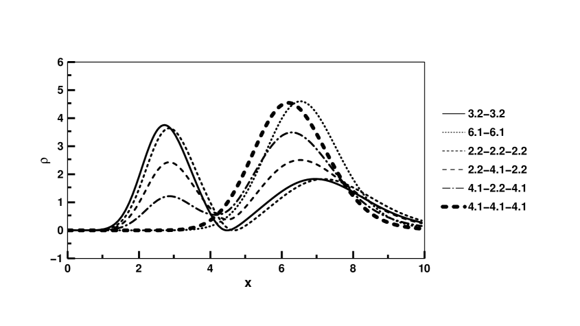
Figure 1: Baryon density of $C^{12}$ shape isomers.

The reason we are looking for possible not pure toroidal solitons is that there is a number of solutions with smaller masses among them. For example a configuration composed from three toroidal multibaryons 3{4.1-4.1-4.1} has a smaller mass. Now this state can not decay into 12 classical skyrmions with $B=1$ ($M_{1\{1.1\}}=11.60608\pi F_{\pi}/e$) or into three toroidal skyrmion with $B=4$ ($M_{1\{4.1\}}=47.67478\pi F_{\pi}/e$). We point such a skyrmion as classically stable configuration. The configuration 3{2.2-2.2-2.2} do not obey the condition of classical stability.

For calculated axially symmetric configurations we present baryon density distributions integrated on $d\Omega=\sin(\theta)d\phi d\theta$ at Figure 1. Here we use dimensionless coordinates $x=F_{\pi}er$.

In according to our calculations the solitons from the same topological sector can have strongly different masses if they have different structure. We also have to point out that a number of the states have shell like structure. There are states which has $n_{i}\neq 1$. Such shape isomer can give different specific contribution to physics processes in light nuclei.

VI Conclusions.

The axially symmetric solitons with baryon number $B=12$ have been investigated in the framework of the very general assumption about the form of the solution of the Skyrme model equations. The obtained solitons could be seen in nuclear reactions as isomer contributions in reactions involving $C^{12}$. Such isomers correspond to different form of baryon density distribution. We have to point out that used ansatz leads to stable solitons with $B=12$ and shell like structure of the baryon density distribution.

VII Acknowledgements.

We thank A.N. Antonov and V.K. Lukyanov for useful discussions of obtained results.
This work is supported in part by the programme ”University of Russia” UR.02.01.020

References

- (1) Skyrme T.H.R. Nucl.Phys. 31, 556 (1962).
- (2) Nikolaev V.A., Novozhilov V.Yu., Tkachev O.G., IL Nuovo Cimento 107(A), 12, 2673 (1994).
- (3) Nikolaev V.A., Tkachev O.G., Proceedings of the Twentieth International Workshop on Nuclear Theory, June 2001, Rila, Bulgaria, Notre Dame Indiana, 167 (2001).
- (4) Nikolaev V.A., Tkachev O.G., hep-ph/0109192 v1 (2001).
- (5) Houghton C.J., Manton N.S. and Sutcliffe P.M., Nucl.Phys. B510, 507 (1998).
- (6) Rychard A. Battye, Paul M.Sutcliffe, hep-th/0012215 v.3 (2001).
- (7) Braaten E., Townsend S., Carson L., Phys.Lett. B235, 147 (1990).
- (8) Weigel H., Schwesinger B., Holzwarth G., Phys. Lett. B168, 556 (1986).
- (9) Kopeliovich V.B., Stern B.E., Pisma v ZhETF 45, 165 (1987).
- (10) Verbaarshot J.J.M.. Phys.Lett. B195, 235 (1987).
- (11) Manton N.S., Phys.Lett. B192, 177 (1987).
- (12) Kozhevnikov I.R., Rybakov Yu.P., Fomin M.B, T.M.F. 75, 353 (1989).
- (13) Nikolaev,V.A., in ”Particles and Nuclei” vol. 20 N2, p.403, Moscow, Atomizdat (1989).
- (14) Nikolaev V.A., Tkachev O.G., JINR Rapid Communications N1[34]-89, p.28, Dubna (1989); N4[37]-89, p.18, Dubna (1989).
- (15) Nikolaev V.A., Nikolaeva R.M., Tkachev O.G., Sov.J.Part.Nucl. 23(2), 239 (1992).
- (16) Nikolaev V.A., Nikolaeva R.M., Tkachev O.G., Sorace E., Tarlini M., Musatov I.V., Physics of Atomic Nuclei 59, 2099 (1996).
- (17) Nikolaev V.A., Tkachev O.G., JINR Preprint E4-89-56, Dubna (1989); TRIUMF (FEW BODY XII), TRI-89-2, p.F25, Vancouver (1989).
- (18) Kurihara T., Kanada H., Otofuji T., Saito S., Progr. of Theor. Phys. 81, p.858 (1989).
- (19) Sorace E., Tarlini M., Phys.Lett. B232, 154 (1989).
- (20) Nikolaev V.A.,Nikolaeva R.M., Tkachev O.G. J.Phys.G: Nucl.Part.Phys 18, 1149 (1992).
- (21) Nikolaev V.A., Nikolaeva R.M., Tkachev O.G., Journal of Nucl. Phys 56(7), 173 (1993).