Jet physics at hadron colliders

Abstract

I give a short summary of jet definition algorithms and recent progress in the quantitative description of jet production.

1 Introduction

Over the last decade detailed theoretical description of jet physics at high energy colliders has been established at the next-to-leading order (NLO) accuracy [1, 2, 3]. The theoretical predictions have been successfully compared with the experimental data in the case of three jet production in $e^{+}e^{-}$ annihilation, one or two jet production in photo-production, deep inelastic scattering at HERA, and one or two jet production at proton-antiproton collisions at Tevatron [4].

Jets are footprints of quarks and gluons produced at short distances. They are defined as some collections of final state hadrons such that the relative angular distances between the hadrons in momentum space are small. Important cancellation theorems valid in all orders of perturbation theory suggest that infrared safe global jet observables can quantitatively be described in terms the weak perturbative dynamics of the point like partons of QCD. A jet observable is infrared safe if it does not change by adding or removing a soft particle from the jet or by splitting an ultra relativistic particle into two collinear particles within the jet.

The data with highest jet energy at Tevatron could give us the most stringent test of the QCD dynamics at short distances and allow for an efficient search for effects of deviations from the Standard Model predictions [5]. The data of CDF and D0 collaborations at Tevatron have about the same ($<20\%$) or better statistical accuracy as the theoretical predictions. At the highest jet energies, the uncertainties in the jet energy calibration and the errors of the fitted values of parton number densities, however, lead up to systematic errors of $\approx 50\%$.

In the case of three jet production in $e^{+}e^{-}$, the experimental systematic errors are smaller and the theoretical uncertainties are considerably larger than the current experimental errors [6]. Therefore the theorists have strong motivations to further improve the accuracy of their predicitons.

Recently, we could witness important theoretical progress in four areas of jet physics. First, the NLO calculations could be extended to 5-leg processes (four jet production in $e^{+}e^{-}$ annihilation [7, 8], three jet production in hadron-hadron collisions [9, 10] etc.). Secondly, remarkable progress has been made towards the ambitious goal of calculating jet cross sections of 4-leg processes in next-to-next-to leading order (NNLO) accuracy [11]. In particular, the NNLO virtual corrections could be calculated analytically for four leg amplitudes. Thirdly, the NLO calculations could be improved in the threshold region by resumming the large logarithmic contributions to all order [12]. Finally new techniques have been developed to calculate many jet processes in leading order[13]. Below I discuss difficulties related to jet definitions, I briefly review the general theoretical framework of the NLO calculations, I describe in some detail the new NLO results obtained for 5-leg processes, finally I summarize the main results on NNLO corrections.

2 Jet definition algorithms

Jet definitions are based on a selection and a recombination algorithm. The selection algorithm selects the group of particles which form the jet and the recombination algorithm specifies how to construct the kinematicl variables of the jet in terms of the momenta of the selected hadrons.

The jet algorithms used in the data analysis are more complicated than the simple theoretical definitions in terms of one, two or three partons. Some ’auxiliary’ features like the phenomena of merging and splitting, or the use of seeds are not always completely specified. These issues may influence the infrared sensitivity and the size of the hadronic fragmention corrections. In a careful analysis one has to require that i) the jet selection process, the jet kinematic variables, preclustering, merging, splitting, the role of the underlying evens are fully specified; ii) The fully specifed algorithm should be infrared safe, independent from the detector properties and the algorithms should be simple to use; iii) The algorithm has to be defined in the same way at parton, hadron and detector level (for a recent detailed discussion for hadron colliders see [14]).

Although the algorithms have a large amount of arbitrariness they should fulfil a number of important theoretical requirements, such as insensitivity to soft radiation and to collinear splitting, or invariance under boost in the case of hadron colliders etc.. In the latter case the use of transverse momentum and rapidities as kinematic variables is preferred. Another constraint is suggested by the study of resummation corrections. Resummations can only be carried out if the boundaries of the inclusive jet kinematic variables are defined independently from the number of final state particles [12, 16]. This prefers Lorenz covariant recombination schemes (such as the E-scheme). Finally, the algorithm should be as simple as possible. At hadron colliders we do not have one best algorithm. The cone algorithm is broadly used while the $k_{T}$ algorithm is preferred more by the theorists.

2.1 Cone jet algorithm for hadron-hadron collisions

The cylindrical shape of the detectors and boost invariance suggest that the kinematics has to be described in terms rapidities and azimuthal angles [2, 3]. In the 2-dimensional $\eta\times\phi$ lego-plot the hadrons or partons constituting the jets lie within a cone of radius R. The trial cone in the lego plot is given by its radius and the value of its center $(\eta^{\rm C}\,,\phi^{\rm C})$. The cone is adjusted in such a way that the geometric center of the cone agrees with the $E_{T}$-weighted recombined values of the particles within the cone. All particles within the trial cone fulfil

$$\sqrt{(\eta^{\rm C}\,-\,\eta_{i})^{2}+(\phi^{\rm C}\,-\,\phi_{i}^{2})}\leq R\,.$$ (1)

A stable cone (protojet) is obtained if the “ physical” center of the cone defined by the recombination algorithm

$$\eta^{\rm R}_{\rm T}=\frac{\sum_{i}\eta^{i}_{\rm T}E^{\rm i}_{\rm T}}{E^{\rm R}_{\rm T}}\,,\quad\quad\phi^{\rm R}_{\rm T}=\frac{\sum_{i}\phi^{i}_{\rm T}E^{\rm i}_{\rm T}}{E^{\rm R}_{\rm T}}\,,\quad\quad E^{\rm R}_{\rm T}=\sum_{i}E^{i}_{\rm T}$$ (2)

coincides with its geometrical center $(\eta^{\rm C}\,,\phi^{\rm C})=(\eta^{\rm R}\,,\phi^{\rm R})$. In this case it is natural to identify the jet variables with the recombined values of the stable cone $(E^{J}_{T},\eta^{\rm J}\,,\phi^{\rm J})=(E^{\rm R}_{T},\eta^{\rm R}\,,\phi^{\rm R})$. After identification of the jet as group of particles within the stable cone one can construct the jet kinematical variables with using some recombination scheme, for example

$$E^{J}_{x,y,z}\,=\,\sum_{i}E^{i}_{x,y,z}$$ (3)

$$\theta^{J}\,=\,\arctan\frac{E^{J}_{T}}{E^{J}_{z}},\quad\quad\phi^{J}\,=\,\arctan\frac{E^{J}_{x}}{E^{J}_{y}},$$ (4)

$$\eta^{J}\,=\,-\ln\left(\tan\frac{\eta^{J}}{2}\right),\quad\quad E^{J}_{T}\,=\,E^{J}\sin\theta^{J}$$ (5)

Different recombination algorithms give aproximately the same kinematical values if $M^{J}<<E^{J}_{T}$. The boost invariant recombination scheme, however, is a better estimator of the jet variables. I have noted above that boost invariant variables are not suitable for resummation studies since the kinematic boundary of the $E^{J}_{T}$ depends on the number of partons. Resummation is consistent with e.g. the E-scheme which recombines the jet four momenta as $p^{J}_{\mu}=\sum_{i}p^{i}_{\mu}$.

If the number of the final states particles are large the method of moving the trial cone gives a slow algorithm. One can speed it up with starting the cone iteration at the center of seed towers which passed a minimum cut-off. But the seeded algorith may have problems with sensitivity to the emission of soft gluons. The algorithm allows for jet overlaps, therefore, one should also specify the details of jet merging and jet splitting. This allows for many ad hoc options and it is difficult to ensure that the definition of jets are the same at the detector and the parton levels. In a quantitative analysis all these details should be treated with great care.

2.2 $k_{T}$ algorithms

The $k_{T}$ algorithm was designed to avoid jet overlaps and problems with kinematical boundaries in the case of resummation [15]. I summarize the version of $k_{T}$ algorithm suggested by Ellis and Soper. The algorithm starts with the initial list of particles and an empty list of jets. Performing the algorithm we get an empty list of particles and the list of jets, each separated by $\Delta R^{2}_{ij}$. This regrouping of particles into jets goes iteratively through five steps.

• Every particle (pseudoparticle) $i$ and every particle pair $(i,j)$ in the particle list is associated with a $d-$value

  $$d_{i}=p^{2}_{i,T}\quad\quad d_{ij}\,=\,{\rm min}(p^{2}_{i,T}\,,\,p^{2}_{j,T})\frac{\Delta R^{2}_{ij}}{D^{2}}$$ (6)

  where $D$ is a free parameter (the usual choice for its value is $D=1$) and $\Delta R^{2}_{ij}$ is the square of the distance between the particles in the lego-plot $\Delta R^{2}_{ij}=(\eta_{i}-\eta_{j})^{2}+(\phi_{i}-\phi_{j})^{2}$.

• Find $d_{\rm min}={\rm min}(d_{i},d_{ij})$.

• If $d_{\min}=d_{ij}$ replace the particle pair $(i,j)$ with a pseudoparticle. Its momentum $p_{ij}$ is calculated via the rules of the recombination scheme. For example using the $E$-scheme $p_{ij}\,=\,p_{i}+p_{j}$.

• If $d_{\min}=d_{i}$ remove particle (pseudoparticle) $i$ from the list of particles and add it to the list of jets.

• If at this step the particle (pseudoparticle) list ist not empty got to step i).

In the experimental analysis the $k_{T}$ algorithm has to combined with some preclustering procedure in order to keep the jet analysis computionally feasible and to diminish the detector dependence of the alghorithm. The $k_{T}$ algorithm has the tendency to reconstruct more energy from calorimeter noise, pile-up and underlying event and multi $p\bar{p}$ interactions than a cone algorithm [14]. The jet momentum resolution appears, however, to be the same for $k_{T}$ jets and cone jets. Therefore, it appears that the use of $k_{T}$ jets has clear overall advantages.

3 NLO cross sections

3.1 Formalism

The lowest order cross-sections strongly depend on the unphysical renormalization and factorization scales. Higher order cross sections reduce this sensitivity with a factor of ${\cal O}({\alpha_{S}})$. The calculation of the NLO corrections is technically involved since the virtual and gluon bremsstrahlung contributions are separately divergent ( soft and collinear singularities). Fortunately, the divergent pieces are universal in the sense that they are given by the Born cross sections times a universal process independent singular factor [2, 3]. The singular parts of the virtual cross sections can be cancelled analytically with contributions of of the real contributions with the use of local counter terms. They are used to subtract the real contributions in the singular soft and collinear regions. This subtraction procedure is consistent with numerical Monte Carlo evaluation of the phase space integrals provided one calculates physical quantities which are defined in terms of infrared safe measurement functions specified below.

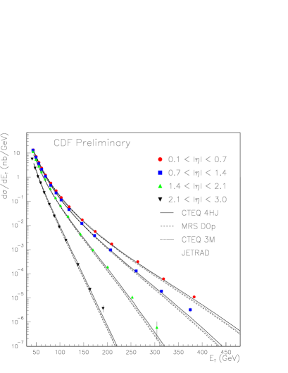
Figure 1: Inclusive jet cross-section [17] as function of the jet energy at various pseudo rapidity intervals. The CDF data are compared with the predictions calculated by the JETRAD NLO MC program [3].

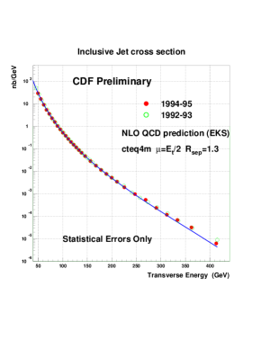
Figure 2: Inclusive jet cross-section as function of the transverse energy measured by the CDF Collaboration [17]. The solid curve is the NLO QCD prediction [2].

In the case of the collisions of hadron A with hadron B, the physical cross section is given in terms of parton number densities $f_{h/H}(x,\mu)$ and parton-parton scattering cross sections $\hat{\sigma}_{a,b}$ as follows

$$\sigma(p_{A},p_{B})=\sum_{a,b}\int dx_{a}dx_{b}f_{a/A}(x_{b},\mu_{F}^{2})f_{b/B}(x_{b},\mu_{F}^{2})$$ (7)

$$\qquad\qquad\qquad\qquad\times\left\{\hat{\sigma}_{a,b}^{LO}(x_{a}p_{A},x_{b}p_{B})+\hat{\sigma}_{a,b}^{NLO}(x_{a}p_{A},x_{b}p_{B})\right\}$$

where for example the LO cross section for the physical quantity ${\cal S}$ is given by the phase space integral over the squared matrix element of the 2-to-n process, weighted by the appropriate measurement function ${\cal S}(p_{a},p_{b};p_{1},...p_{n})$

$$\hat{\sigma}_{a,b}^{LO}(p_{a},p_{b};[{\cal S}^{(}n)])=\int_{n}d\hat{\sigma}_{a}^{B}(p_{a},p_{b})=\int d\Gamma^{(n)}|M_{a,b}|^{2}{{\cal S}^{(n)}(p_{a},p_{b},p_{1},..,p_{n})}$$

The finite parton cross sections in NLO are obatained by summing the virtual, real and counter term contributions

$$\hat{\sigma}_{a}^{NLO}(p_{a},p_{b})=\int_{n+1}\hat{\sigma}_{a,b}^{R}(p_{a},p_{b})+\int_{n}\hat{\sigma}_{a,b}^{V}(p_{a},p_{b})+\int_{n}\hat{\sigma}_{a,b}^{\rm col}(p_{a},p_{b})$$

The individual contributions are evaluated in d-dimension. In the numerical evaluation of the phase space integral over the real part we need to subtract the singular contributions locally. Fortunately there are several general methods for constructing such local subtarction terms analytically [2, 3, 16]. We can write

$$d\sigma_{a,b}^{NLO}=\left\{d\sigma_{a,b}^{R}-d\sigma_{a,b}^{\rm loc}\right\}+d\sigma_{a,b}^{\rm loc}+d\sigma_{a,b}^{V}+d\sigma_{a,b}^{\rm col}\;\;,$$

The local subtraction term $d\sigma_{a,b}^{\rm loc}$ is a suitable approximation of $d\sigma_{a,b}^{R}$. They become equal in the singular regions. In order to cancel analytically the singular parts of the virtual contributions we must be able to carry out analytically the integrals over the single parton subspaces in $d=2-2\epsilon$ dimension. After performing this integration over the local subtraction terms the singular pieces of the terms in eq. (3.1) can be cancelled analytically and the remaning part can be evaluated numerically in four dimensions.

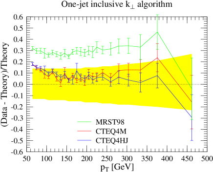
Figure 3: Comparison of the data and the theory in the case of inclusive jet production. Jets are defined by the the $k_{T}$ algorithm [17].

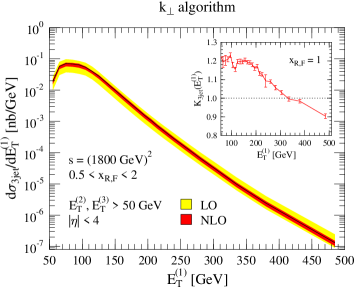
Figure 4: Theoretical prediction for inclusive three jet production at the Tevatron ( Z. Nagy [9]). The band indicate the theoretical uncertainty due to the variation of the renormalization and factorization scales $x_{R,F}$ between 0.5 and 2. The inset shows the K-factor.

The cancellation mechanism of the soft and collinear singularities of the virtual corrections against the singular part of the real contribution is independent of the form of the measurement functions provided that they are insensitive to collinear splitting and soft emission. That is in the soft or/and collinear configurations the measurement functions must fulfil the condition

$${\cal S}^{(n+1)}(p_{a},..p_{n+1})={\cal S}^{(n)}(\tilde{p}_{a},...\tilde{p}_{n})$$ (8)

The existence of universal local subtraction terms [2, 3, 16] is crucial for the method. The most widely used implementation is the one by Catani and Seymour[16]. The construction of the NLO parton level Monte Carlo programs for 4-leg processes is by now a routine (although rather laborious) work. The success of the NLO description of jet production at hadron colliders is well illustrated by the plots shown figures 1 and 2. We see a spectacular agreement in a wide range of kinematical variables. The ambiguities due to errors in the parton number densities are shown in figure 3.

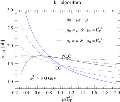
Figure 5: Comparison of the scale dependence of the three jet cross sections obtained in LO and NLO accuracy [9].

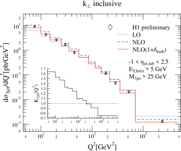
Figure 6: The NLO prediction for differential (3+1)-jet cross-section in the range $5<Q^{2}<5000\,{\rm GeV}^{2}$ is compared with the data of the H1 collaboration [19].

4 NLO description of 5-leg process

4.1 New results for $e^{+}e^{-}$

The final experimental analysis of 4-jet production and its comparison with the NLO theoretical predictions was recently completed [18]. The most remarkable result is that we obtain a more precise measurement of the strong coupling constant from the analysis of the 4-jet data than from the 3-jet data. This is not completely suprising since the cross section of four jet production is more sensitive to $\alpha_{s}$ than the three jet cross section, furthemore due to the large number of events the statistical accuracy is not the dominating the experimental error.

4.2 New results for $pp(\bar{p})$ and $ep$ scattering

Important progress in this topics is that the theoretical results [7] (where the singularities are not manifestly cancelled) could be implemented in a efficient parton level C++ Monte Carlo program (called NLO++ ) both for $ep$ [19] and for $pp(\bar{p})$ [9] scattering. Similarly to the case of $e^{+}e^{-}$ annihilation, the accuracy of the theoretical prediction is greatly improved. This is illustrated in figure 4 and 5. In fig. 4 inclusive jet cross section for three jet production is plotted using the $k_{T}$ algorithm. As we mentioned above, in multi jet production the use of the cone algorithm is cumbersome. It is assumed that the jets are produced in the pseudo rapidity interval $\left|\eta\right|<4$ and at energy of $\sqrt{s}=1800\,{\rm GeV}$, with minimum transverse jet energy $E_{T}>50\,{\rm GeV}$. The cross section is plotted as a function of the transverse energy of the leading jet $E_{T}^{(1)}$. The hard scattering factorization and renormalization scale is chosen to be $E_{T}^{(1)}$. The theoretical ambiguity is indicated as a band when the hard scattering scale is changed by a factor in the range $0.5<x_{R,F}<2$. One can see that at NLO the cross section values show much less sensitivity to the value of the hard scattering scale as the LO cross sections. Hopefully, these predictions can be compared with the Tevatron data in the near future. In fig. 5 integrated cross section values of three jet production (with the same kinematics as in fig. 4 but integrated over $E_{T}^{(1)}>100\,{\rm GeV}$) are plotted as a function of the ratio $\mu/E_{T}^{(1)}$ where $\mu$ is the value of the hard scattering scale.

Due to crossing symmetry the $e^{+}e^{-}$ NLO four jet matrix elements allow also the evaluation of the DIS 3+1 jet processes at NLO. The implementation of the matrix elements [7] into C++ Monte Carlo program with the corresponding local subtraction terms has been recently carried out [19]. The new result is crucial in the quantitative comparison of the data with the theory. As one can see in fig. 6, at NLO, we get substantial reduction in the precision of the theoretical prediction and at the same time the large NLO corrections are needed to bring the data in agreement with the theory.

5 NNLO calculations

In the last few years, the most spectacular progress has been achieved in developing the technics of calculating cross section values at NNLO accuracy. This requires the analytic computation of two loop corrections to 4-leg QCD processes (for a recent more complete review see [11].) The basic ingredient behind this success is the use of two technical tricks. First, if one uses integration by parts [20] and Lorenz invariance [21] identities one can reduce the very large number of different integrals into a few master integrals. This step can be very well computerized and by now several computer algorithms are available which perform automatically this reduction. Second, all the remaining master integrals (double box diagrams, etc.) could be evaluated analytically. Three different methods have been used: i) Mellin-Barnes integral transformations [22]; ii)  inhomogeneous linear differential equations [21] and iii) expansions in terms of nested harmonic sums [23]. In addition, the integrals could be calculated numerically using sector decomposition [24]. Very recently, the differential equation method could be extended also to phase space integrals [25]. New classes of functions appear in the final solutions. Numerical algorithms are available for the fast evaluation of these functions. All parton-parton scattering amplitudes could be calculated analytically at two loop order. Analytic expressions of the virtual corrections to the cross sections of three jet production in $e^{+}e^{-}$ annihilation have been published recently [27]. As a first phenomenological application Bern et.al. [26] have computed the cross section of two photon production at LHC in NNLO accuracy. In the case of this process the treatment of the bremsstrahlung corrections are considerable easier than in the general case. For processes involving initial hadrons, the parton evolution has to be evaluated also at NNLO accuracy. The results for the non-singlet case have been published recently by Moch and Vermaseren. This is an outstanding technical achievement. If the NNLO splitting functions [28] will be known the fitting of the initial parton density functions can be carried out at NNLO accuracy. Depending on the nature of the Beyond the Standard Model Physics, the newly achieved theoretical results may be crucial for the success of the experimental programs at future collider experiments. The impact of these developments can not be overestimated for the future high precision measurements at HERA, Tevatron, LHC and TESLA.

References

- [1] R. K. Ellis, D. A. Ross and A. E. Terrano, Nucl. Phys. B 178 (1981) 421; MC implementation: Z. Kunszt, P. Nason (Zurich, ETH) LEP Physics Wrkshp.1989:v.1:373-453 (QCD161:L39:1989).
- [2] S. D. Ellis, Z. Kunszt and D. E. Soper, Phys. Rev. Lett. 64 (1990) 2121; Z. Kunszt and D. E. Soper, Phys. Rev. D 46 (1992) 192.
- [3] W. T. Giele and E. W. Glover, Phys. Rev. D 46, 1980 (1992). W. T. Giele, E. W. Glover and D. A. Kosower, Phys. Rev. Lett. 73 (1994) 2019 W. T. Giele, E. W. Glover and D. A. Kosower, Nucl. Phys. B 403 (1993) 633.
- [4] R. K. Ellis, J. W. Stirling and B. R. Webber ” QCD and collider physics”, Cambridge Monogr.Part.Phys.Nucl.Phys.Cosmol.8 :1-435,1996.
- [5] J. Huston “QCD At High-Energy”, Proceedings of the 29th International Conference on High-Energy Physics (ICHEP 98), in Vancouver 1998, High energy physics, vol. 1* 283-302. (Eds.: A. Astbury et.al., World Scientific).
- [6] S. Bethke,Workshop, RADCOR98, Barcelona, hep-ex/9812026.
- [7] Z. Bern (UCLA), L. J. Dixon, D. A. Kosower, Nucl.Phys.B513:3-86,1998.
-
[8]
L. J. Dixon and A. Signer,
Phys. Rev. D 56 (1997) 4031;
A. Signer and L. J. Dixon,
Phys. Rev. Lett. 78 (1997) 811;
Z. Nagy and Z. Trocsanyi, Phys. Rev. D 59 (1999) 014020 [Erratum-ibid. D 62 (2000) 099902]. - [9] Z. Nagy, Phys. Rev. Lett. 88 (2002) 122003, hep-ph/0110315; W. B. Kilgore and W. T. Giele, hep-ph/0009193.
- [10] Z. Bern, L. J. Dixon, and D. A. Kosower, Phys. Rev. Lett. 70, 2677 ( 1993); Z. Bern, L. J. Dixon, and D. A. Kosower, Nucl. Phys. B437, 259 ( 1995); Z. Kunszt, A. Signer, and Z. Trócsányi, Phys. Lett. B336, 529 ( 1994).
- [11] T. Gehrmann, Talk given at the RADCOR2002 Workshop, hep-ph/0210157.
- [12] G. Sterman and W. Vogelsang, arXiv:hep-ph/0002132; R. Bonciani, S. Catani, M. L. Mangano and P. Nason, Nucl. Phys. B 529 (1998) 424 arXiv:hep-ph/9801375.
- [13] M. L. Mangano, M. Moretti, F. Piccinini, R. Pittau and A. D. Polosa,
- [14] S.D. Ellis, J. Huston, M. Tonnesmann [aXiv:hep-ph/0111434]; G. Blazey et.al. [aXiv:hep-exp/0005012].
- [15] S. Catani, Y. L. Dokshitzer, M. H. Seymour, and B. R. Webber, Nucl. Phys. B406, 187 ( 1993); S. D. Ellis and D. E. Soper, Phys. Rev. D 48 (1993) 3160.
- [16] S. Catani and M. H. Seymour, Nucl. Phys. B485, 291 ( 1997), Erratum-ibid B 510, 503 (1997); see also S. Frixione, Z. Kunszt, and A. Signer, Nucl. Phys. B467, 399 ( 1996); Z. Nagy and Z. Trócsányi, Nucl. Phys. B486, 189 ( 1997).
- [17] F. Abe et al. [CDF Collaboration], Phys. Rev. Lett. 77 (1996) 438.
- [18] G. Dissertori, arXiv:hep-ex/0209070.
- [19] Z. Nagy and Z. Trocsanyi, Phys. Rev. Lett. 87 (2001) 082001 [arXiv:hep-ph/0104315].
- [20] F.V. Tkachov, Phys. Lett. 100B (1981) 65; K.G. Chetyrkin and F.V. Tkachov, Nucl. Phys. B192 (1981) 159.
- [21] T. Gehrmann and E. Remiddi, Nucl. Phys. B580 (2000) 485.
- [22] V.A. Smirnov, Phys. Lett. B460 (1999) 397, ibid B491 (2000) 130, ibid B500 (2001) 330; J.B. Tausk, Phys. Lett. B469 (1999) 225.
- [23] S. Moch, P. Uwer and S. Weinzierl, J. Math. Phys. 43 (2002) 3363; S. Weinzierl, Comput. Phys. Commun. 145 (2002) 357.
- [24] T. Binoth and G. Heinrich, Nucl. Phys. B585 (2000) 741.
- [25] C. Anastasiou and K. Melnikov, hep-ph/0207004.
- [26] Z. Bern, L. Dixon and C. Schmidt, hep-ph/0206194.
- [27] L.W. Garland, T. Gehrmann, E.W.N. Glover, A. Koukoutsakis and E. Remiddi, Nucl. Phys. B627 (2002) 107; ibid B642 (2002) 227.
- [28] S. Moch, J. A. Vermaseren and A. Vogt, Nucl. Phys. B 646 (2002) 181.