General Structure of Relativistic Vector Condensation

Abstract

We study relativistic massive vector condensation due to a non zero chemical potential associated to some of the global conserved charges of the theory. We show that the phase structure is very rich. More specifically there are three distinct phases depending on the value of one of the zero chemical potential vector self interaction terms. We also develop a formalism which enables us to investigate the vacuum structure and dispersion relations in the spontaneously broken phase of the theory. We show that in a certain limit of the couplings and for large chemical potential the theory is not stable. This limit, interestingly, corresponds to a gauge type limit often employed to economically describe the ordinary vector mesons self interactions in QCD. We finally indicate for which physical systems our analysis is relevant.

I Introduction

Relativistic vector condensation has been proposed and studied in different realms of theoretical physics. However the condensation mechanism and the nature of the relativistic vector mesons themselves is quite different. Linde Linde:1979pr , for example, proposed the condensation of the intermediate vector boson $W$ in the presence of a superdense fermionic matter while Ambjørn and Olesen Ambjorn:1989gb investigated their condensation in presence of a high external magnetic field. Manton Manton:1979kb and later on Hosotani Hosotani:1988bm considered the extension of gauge theories in extra dimensions and suggested that when the extra dimensions are non simply connected the gauge fields might condense. Li in Li:2002iw has also explored a simple effective Lagrangian and the effects of vector condensation when the vectors live in extra space dimensions.

Brown and Rho Brown:kk also suggested that the non gauge vectors fields such as the (quark) composite field $\rho$ in QCD may become light and possibly condense in a high quark matter density and/or in hot QCD. Harada and Yamawaki’s Harada:2000kb dynamical computations within the framework of the hidden local gauge BKY symmetry support this picture.

Rotational symmetry can also break in a color superconductor if two quarks of the same flavor gap. In this case the quarks must pair in a spin one state and a careful analysis has been performed in Pisarski:1999tv . Whether this gap occurs or not in practice is a dynamical issue recently investigated in Buballa:2002wy .

We consider another type of condensation. If vectors themselves carry some global charges we can introduce a non zero chemical potential associated to some of these charges. If the chemical potential is sufficiently high one can show that the gaps (i.e. the energy at zero momentum) of these vectors become light Lenaghan:2001sd ; Sannino:2001fd and eventually zero signaling an instability. If one applies our results to 2 color Quantum Chromo Dynamics (QCD) at non zero baryon chemical potential one predicts that the vectors made out of two quarks (in the 2 color theory the baryonic degrees of freedom are bosons) condense. Recently lattice studies for 2 color at high baryonic potential Alles:2002st seem to support our predictions. This is the relativistic vectorial Bose-Einstein condensation phenomenon. A decrease in the gap of vectors is also suggested at high baryon chemical potential for two colors in Muroya:2002ry .

Interestingly non-relativistic vectorial Bose-Einstein condensation recently has attracted much attention in condensed matter physics since it has been observed experimentally in alkali atom gases VBE . We also note that in this framework a rich phenomenology related to the classical solutions of the theory, such as vortices Volovik:2000mt , is expected to occur.

Here we extend the analysis presented in Lenaghan:2001sd ; Sannino:2001fd by showing the existence of new phases while providing a detailed investigation of the relativistic massive vector condensation phenomenon driven by a non zero chemical potential. We develop an efficient formalism which allows us to analytically study the dispersion relations of the vectors in the broken phase of the theory and set the stage for possible higher order computations. Our Lagrangian approach has to be understood as a Landau theory describing the vector condensation phenomenon.

Having in mind some specific physical applications we assume our massive relativistic vectors to be in the adjoint representation of the non abelian $SU(2)$ global symmetry group. We then turn on a chemical potential in a specific $SU(2)$ direction which breaks $SU(2)$ explicitly to a $U(1)$ symmetry. We demonstrate that we can have three independent phases according to the value assumed by one of the two distinct (non derivative) vector self interactions. The polar phase, the apolar phase and the enhanced symmetry one. The polar phase has been introduced in Sannino:2001fd along with the enhanced symmetry case. The polar and apolar phases are the relativistic generalization of the phases encountered in the condense matter Volovik:2000mt framework. The appearance of a given phase is related to the specific value of one of the vector self interaction coefficients of the Lagrangian at zero chemical potential. In this paper we study consistently the gapless excitations and the dispersion relations in all of the phases while providing a formalism helpful when trying to go beyond the tree level approximation.

In the polar phase the vector condensate breaks the rotational symmetry down to a simple rotation around the axis of condensation. The internal $U(1)$ symmetry breaks completely as well. This phase is characterized by three gapless excitations with linear in momentum dispersion relations. By studying in detail the dispersion relations we show that two of the gapless states have isotropic dispersion relations while the third excitation has different velocities in the direction parallel and orthogonal to the vacuum expectation value. The detailed analysis of the dispersion relations is exact when we supplement the global symmetry $SU(2)$ by an extra one which allows only an even number of vectors in any vertex of the theory, however the number and type of goldstone bosons is independent of the extra discrete symmetry.

If we are in the apolar phase the condensation of the vector is such that the unbroken generator is a linear combination of one of the rotational generators and the abelian $U(1)$ generator. Only two gapless excitations emerge this time. One with linear and the other with quadratic dispersion relations. However the vacuum still breaks three generators. This is in agreement with the Nielsen and Chadha Nielsen counting scheme according to which in absence of Lorentz invariance (and under a number of assumptions) each gapless excitation with quadratic dispersion relations has to be counted as two goldstone bosons with linear dispersion relations. More specifically if $n_{I}$ denotes the number of gapless excitations of type $I$ with linear dispersion relations (i.e. $E\propto p$) and $n_{II}$ the ones with quadratic dispersion relations (i.e. $E\propto p^{2}$) the Goldstone theorem generalizes to $n_{I}+2\,n_{II}\geq\#~{}{\rm broken~{}generators}$. Clearly in the absence of type $II$ excitations we recover the usual counting. We analyze the spectrum in this case and find that the type II goldstone boson has isotropic dispersion relations while the type I has not. In all of the phases the non goldstone boson excitations are investigated in detail as well.

If one of the self-vector couplings is set to zero we observe three gapless excitations: 2 type II goldstone bosons and one type I. In this case the potential has an enhanced global symmetry, i.e. it has an $SO(6)$ which the vacuum breaks to an $SO(5)$. In absence of Lorentz breaking, we would have 5 ordinary goldstone bosons. However the presence of the chemical potential in the derivative terms of the Lagrangian prevents the emergence of 2 extra goldstone bosons Schafer:2001bq while turning 2 goldstones into type II Sannino:2001fd .

We also discover that when the vector self interaction couplings are tuned to be the ones predicted using the Yang-Mills relation (while keeping always a non zero vector mass) the theory at high chemical potential does not predict a stable solution. The existence of an inhomogeneous phase is not excluded. However a more natural solution of the instability is that the chemical potential, when increasing the associated charge density, is at the most as large as the mass of the vectors.

If we now apply our results to describe non elementary relativistic massive vectors such as the $\rho$ field of QCD at high chemical potential (isospin for example) it will help elucidating and constructing the effective Lagrangians for vector fields at zero chemical potential. Interestingly, indeed, the particular choice of the vector coupling respecting Yang-Mills relations is the one often assumed in literature when introducing the quark composite field $\rho$ at the effective Lagrangian level KRS ; KS . For example the gauge choice of the couplings emerges very naturally when the vector mesons are introduced as gauge fields of an hidden local gauge symmetry BKY . By studying the vector condensation phenomenon (for example the ordinary $\rho$ at high isospin chemical potential) on the lattice it is possible to shed light on the correct way of constructing a theory for composite vector fields or massive vector fields in general. These effective theories for composite fields are relevant also for the physics beyond the standard model of particle interactions such as the ones relative to a strongly interacting electroweak sector (see ARS ; DRS ).

In section II we present the Lagrangian and study the vacuum. We show that a number of phases can be present. In sec. III we solve for the dispersion relations. We then conclude while reviewing the physical applications in sec. IV. In the appendices we summarize first all of the terms of the Lagrangian in the cartesian and cylindrical coordinates. We finally show the computational details of the dispersion relations for the apolar case.

II Vacuum Structure and Different Phases

There are different ways to describe vector fields at the effective Lagrangian level. For example one can use the hidden local gauge symmetry of Ref. BKY , or the antisymmetric tensor field of Ref. Ecker:1993de . Or one can introduce the massive vector fields following the method outlined in KRS ; KS . For most of the known physical applications these approaches provide identical results (at the tree level). It is worth noticing that in some of these methods certain coefficients of the vector Lagrangian are related by enforcing the Yang-Mills relations.

We choose to consider the following general effective Lagrangian for a relativistic massive vector field in the adjoint of $SU(2)$ in $3+1$ dimensions and up to four vector fields, two derivatives and containing only intrinsic positive parity terms:

$${\cal L} = -\frac{1}{4}F^{a}_{\mu\nu}F^{a{\mu\nu}}+\frac{m^{2}}{2}A_{\mu}^{a}A^{a\mu}+\delta\,\epsilon^{abc}\partial_{\mu}A_{a\nu}A^{\mu}_{b}A^{\nu}_{c}-\frac{\lambda}{4}\left(A^{a}_{\mu}A^{a{\mu}}\right)^{2}+\frac{\lambda^{\prime}}{4}\left(A^{a}_{\mu}A^{a{\nu}}\right)^{2}\ ,$$ (1)

with $F_{\mu\nu}^{a}=\partial_{\mu}A^{a}_{\nu}-\partial_{\nu}A^{a}_{\mu}$, $a=1,2,3$ and metric convention $\eta^{\mu\nu}={\rm diag}(+,-,-,-)$. Here, $\delta$ is a real dimensionless coefficient, $m^{2}$ is the tree level mass term and $\lambda$ and $\lambda^{\prime}$ are positive dimensionless coefficients with $\lambda\geq\lambda^{\prime}$ when $\lambda^{\prime}\geq 0$ or $\lambda\geq 0$ when $\lambda^{\prime}\geq 0$ to insure positivity of the potential. The Lagrangian describes a self interacting $SU(2)$ Yang-Mills theory in the limit $m^{2}=0$, $\lambda=\lambda^{\prime}>0$ and $\delta=-\sqrt{\lambda}$.

It is relevant to notice that in the limit $\delta=0$ the theory gains a new symmetry according to which we have always a total number of even vectors in any process. This symmetry guarantees that if the $\delta$ term is absent from the start it will not be generated dynamically. In this paper we will mainly investigate the theory in this case since it will simplify our computations. However we will comment on the effects of such a term in a final paragraph.

The effect of a nonzero chemical potential associated to a given conserved charge - (say $\displaystyle{T^{3}=\frac{\tau^{3}}{2}}$) - can be readily included Lenaghan:2001sd by modifying the derivatives acting on the vector fields:

$$\partial_{\nu}A_{\rho}\rightarrow\partial_{\nu}A_{\rho}-i\left[B_{\nu}\ ,A_{\rho}\right]\ ,$$ (2)

with $B_{\nu}=\mu\,\delta_{\nu 0}T^{3}\equiv V_{\nu}T^{3}$ where $V=(\mu\ ,\vec{0})$. In appendix it is summarized the effective Lagrangian, in this basis, after the introduction of the chemical potential. The introduction of the chemical potential breaks explicitly the Lorentz transformation leaving invariant the rotational symmetry. Also the $SU(2)$ internal symmetry breaks to a $U(1)$ symmetry. If the $\delta$ term is absent we have an extra unbroken $Z_{2}$ symmetry which acts according to $A^{3}_{\mu}\rightarrow-A^{3}_{\mu}$. These symmetries suggest introducing the following cylindric coordinates:

$$\phi_{\mu} = {1\over\sqrt{2}}(A^{1}_{\mu}+iA^{2}_{\mu})\ ,\qquad\phi^{\ast}_{\mu}={1\over\sqrt{2}}(A^{1}_{\mu}-iA^{2}_{\mu})\ ,\qquad\psi_{\mu}=A^{3}_{\mu}\ ,$$ (3)

on which the covariant derivative acts as follows:

$$D_{\mu}\phi_{\nu}=\left(\partial+i\,V\right)_{\mu}\phi_{\nu}\ ,\quad D_{\mu}\psi_{\nu}=\partial_{\mu}\psi_{\nu}\ ,\quad V_{\nu}=\left(\mu,{\bf 0}\right)\ .$$ (4)

The quadratic, cubic and quartic terms - in the vector fields - in the cylindrical coordinates are summarized in the appendices.

II.1 The Non Derivative Terms

We first study the non derivative terms which we collect in the following potential type term:

$$V = -\frac{m^{2}}{2}\left[2{\phi^{\ast 0}}\phi^{0}+\psi\cdot\psi\right]+\left(m^{2}-\mu^{2}\right)\,\left[{\phi^{\ast 0}}\phi^{0}-\phi^{\ast}\cdot\phi\right]+{2\lambda-\lambda^{\prime}\over 2}(\phi^{\ast}\cdot\phi)^{2}-{\lambda^{\prime}\over 2}|(\phi\cdot\phi)|^{2}+{\lambda-\lambda^{\prime}\over 4}(\psi\cdot\psi)^{2}$$ (5)

$$+{\lambda}(\phi^{\ast}\cdot\phi)(\psi\cdot\psi)-\lambda^{\prime}|(\psi\cdot\phi)|^{2}+2\mu\delta\,\psi^{0}\left(\phi^{\ast}\cdot\phi\right)+\mu\delta\,\left[{\phi^{\ast}}^{0}\left(\phi\cdot\psi\right)+{\rm c.c.}\right]\ .$$

We can read off the symmetries of the theory from the potential. When $\delta=0$, for example, we gain the discrete symmetry $\psi\rightarrow-\psi$. To explore the vacuum structure of the theory we consider the following variational ansatz:

$$\psi^{\mu}=0\ ,\qquad\phi^{\mu}=\sigma\,\left(\begin{array}[]{c}0\\ 1\\ e^{i\alpha}\\ 0\\ \end{array}\right)\ .$$ (10)

Substituting the ansatz in the potential expression we have:

$$V=2\,\sigma^{4}\left[(2\lambda-\lambda^{\prime})-\lambda^{\prime}\cos^{2}\alpha\right]+2\left(m^{2}-\mu^{2}\right)\sigma^{2}\ .$$ (11)

The potential is positive for any value of $\alpha$ when $\lambda>\lambda^{\prime}$ if $\lambda^{\prime}\geq 0$ or $\lambda>0$ if $\lambda^{\prime}<0$. Due to our ansatz the ground state is independent of $\delta$. The unbroken phase occurs when $\mu\leq m$ and the minimum is at $\sigma=0$. A possible broken phase is achieved when $\mu>m$ since in this case the quadratic term in $\sigma$ is negative. According to the value of $\lambda^{\prime}$ we distinguish three distinct phases:

II.2 The polar phase: $\lambda^{\prime}>0$

In this phase the minimum is for

$$\langle\phi^{\mu}\rangle=\sigma\,\left(\begin{array}[]{c}0\\ 1\\ 1\\ 0\\ \end{array}\right)\ ,\quad{\rm with}\quad\sigma^{2}=\frac{1}{4}\frac{\mu^{2}-m^{2}}{\lambda-\lambda^{\prime}}\ ,$$ (16)

This phase has been partially analyzed in Sannino:2001fd . We have the following pattern of symmetry breaking $SO(3)\times U(1)\rightarrow SO(2)$. If we define with ${R_{i}}$ the three generators of $SO(3)$ (acting only on the spatial indices) as follows:

$$R_{1}=\left(\begin{array}[]{ccc}0&1&0\\ -1&0&0\\ 0&0&0\\ \end{array}\right)\ ,\quad R_{2}=\left(\begin{array}[]{ccc}0&0&1\\ 0&0&0\\ -1&0&0\\ \end{array}\right)\ ,\quad R_{3}=\left(\begin{array}[]{ccc}0&0&0\\ 0&0&1\\ 0&-1&0\\ \end{array}\right)\ ,$$ (26)

while the $U(1)$ generator acts as a phase on $\phi$ then the unbroken generator determined imposing invariance of the vacuum

$$T_{\rm unbroken}^{\rm polar}\langle\phi\rangle=0\ ,$$ (27)

is the linear combination $T_{\rm unbroken}^{\rm polar}=R_{2}-R_{3}$. We have three broken generators. We can show (see section on the dispersion relations for details) that in this case we have 3 gapless excitations with linear dispersion relations. All of the physical states (with and without a gap) are either vectors (2-component) or scalars with respect to the unbroken $SO(2)$ group. The dispersion relations for the 3 gapless states Sannino:2001fd computed explicitly in the following sections are reported here for the reader’s convenience.

$$E^{2}_{\Phi_{V}^{-}} \propto {\lambda^{\prime}}(\mu^{2}-m^{2})\,{\bf p}^{2}\ ,\qquad\qquad{\rm~{}~{}~{}~{}~{}~{}~{}V=2~{}Physical~{}States}$$ (28)

$$E_{{\Phi_{S}}^{-}}^{2} \propto (\mu^{2}-m^{2})\,\left(p^{2}_{\perp}+{v}_{{\Phi_{S}}^{-}_{\parallel}}^{2}p^{2}_{\parallel}\right)\ ,\quad{\rm S=1~{}Physical~{}State}$$ (29)

$${v}_{{\Phi_{S}}^{-}_{\parallel}}^{2} \propto \left(\lambda-\lambda^{\prime}\right)\frac{\mu^{2}\,\lambda+\lambda^{\prime}\left(\mu^{2}-2m^{2}\right)}{(\mu^{2}\lambda-m^{2}\lambda^{\prime})^{2}}\ ,$$ (30)

where $p_{\parallel(\perp)}$ refers to the momentum parallel (orthogonal) to the vacuum. Here we present the leading terms in a momentum expansion of the gapless dispersion relations. The vector components orthogonal to the vacuum direction (2 states indicated with $V$) propagate isotropically while the component in the direction of the vacuum (1 state indicated with $S$) does not. As a consistency check one sees that at $\mu=m$ the dispersion relations are all isotropic. At $\mu=m$ the dispersion relations are no longer linear in the momentum. This is related to the fact that the specific part of the potential term has a partial conformal symmetry discussed first in Sannino:2001fd . Some states in the theory are curvatureless but the chemical potential term present in the derivative term prevents these states to be gapless. There is a transfer of the conformal symmetry information from the potential term to the vanishing of the velocity of the gapless excitations related to the would be gapless states. This conversion is due to the linear time-derivative term induced by the presence of the chemical potential term Schafer:2001bq ; Sannino:2001fd .

II.3 Enhanced symmetry and type II Goldstone bosons: $\lambda^{\prime}=0$

Here the potential has an enhanced $SO(6)$ in contrast to the $SU(2)\times U(1)$ for $\lambda^{\prime}\neq 0$ global symmetry which breaks to an $SO(5)$ with 5 broken generators. Expanding the potential around the vacuum we find 5 null curvatures Sannino:2001fd . However we have only three gapless states obtained diagonalizing the quadratic kinetic term and the potential term (see the dispersion relation section). Two states (a vector of $SO(2)$) become type II goldstone bosons (see eq. (28)) while the scalar state remains type I. This latter state is the goldstone boson related to the spontaneously broken $U(1)$ symmetry. According to the Nielsen-Chada theorem the type II states are counted twice with respect to the number of broken generators while the linear just once recovering the number of generators broken by the vacuum. More specifically one can prove Sannino:2001fd that the velocity of the states labelled by $V$ in eq. (28) is proportional to the curvatures (evaluate on the minimum) of the would be goldstone bosons which is zero in the $\lambda^{\prime}=0$ limit. Again we have an efficient mechanism for communicating the information of the extra broken symmetries from the curvatures to the velocities of the already gapless excitations.

II.4 The apolar phase: $\lambda^{\prime}<0$

We now extend the vacuum analysis in Sannino:2001fd to the apolar phase in which the potential is minimized for:

$$\langle\phi^{\mu}\rangle=\sigma\,\left(\begin{array}[]{c}0\\ 1\\ \imath\\ 0\\ \end{array}\right)\ ,\quad{\rm with}\quad\sigma^{2}=\frac{1}{2}\frac{\mu^{2}-m^{2}}{2\lambda-\lambda^{\prime}}\ .$$ (35)

In this phase we have again 3 broken generators. However the unbroken generator is the following combination of the $U(1)$ and $SO(3)$ generator:

$$T_{\rm unbroken}^{\rm apolar}=R_{1}-i\,{\bf 1}\ .$$ (36)

More explicitly the action on the vev is $(R_{1}-\imath\,{\bf 1})\langle\phi\rangle=0$. In this phase as we shall demonstrate in the next sections we have only two gapless states. One of the two states is a type I goldstone boson while the other is type II. The two goldstone bosons are one in the $z$ and the other in the $x-y$ plane. Interestingly in this phase, due to the intrinsic complex nature of the vev, we have spontaneous $CP$ breaking.

We summarize in Fig. 1 the phase structure in terms of the number of goldstone bosons and their type according to the values assumed by $\lambda^{\prime}$.

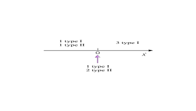
Figure 1: We show the number and type of goldstone bosons in the three distinct phases associated to the value assumed by the coupling $\lambda^{\prime}$. In the polar phase, positive $\lambda^{\prime}$, we have 3 type I goldstone bosons. In the apolar phase, negative $\lambda^{\prime}$, we have one type I and one type II goldstone boson while in the enhanced symmetry case $\lambda^{\prime}=0$ we have one type I and two type II excitations.

II.5 The case $\lambda=\lambda^{\prime}$: the gauge theory limit

Here the potential is:

$$V=2\,\sigma^{4}\lambda\sin^{2}\alpha+2\left(m^{2}-\mu^{2}\right)\sigma^{2}\ .$$ (37)

This potential has two extrema when $\mu>m$, one for $\alpha=0$ and $\sigma=0$ which is an unstable point and the other for $\alpha=\pm\pi/2$ and $\sigma^{2}=\frac{(\mu^{2}-m^{2})}{2\lambda}$ corresponding to a saddle point (see the potential in Fig. 2).

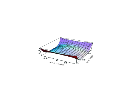
Figure 2: Potential plotted for $\mu=2m$ and $\lambda=\lambda^{\prime}=1$.

At first the fact that we have no stable solutions seems unreasonable since we know that in literature we often encounter condensation of intermediate vector mesons such as the $W$ boson. However (except for extending the theory in higher space dimensions) in these cases one often introduces an external source. For example one adds to the theory a strong magnetic field (say in the direction $z$) which couples to the electromagnetically charged intermediate vector bosons $W^{+}$ and $W^{-}$). In this case the potential is (see Ambjorn:1989gb ):

$$V=2\,\sigma^{4}\lambda\sin^{2}\alpha+2\left(m^{2}-e\,H\,\sin\alpha\right)\sigma^{2}\ ,$$ (38)

where $e$ is the electromagnetic charge and $H$ is the external electromagnetic source field. This potential has a true minimum for $\alpha=\pi/2$ and $\sigma=\frac{eH-m^{2}}{2\lambda}$ whenever the external magnetic field satisfies the relation $eH>m$. We learn that the relativistic vector theory is unstable at large chemical potential whenever the non derivative vector self interactions are tuned to be identical. This is precisely the limit often used in literature when writing effective Lagrangians that in QCD describe the $\rho$ vector field. In principle we can still imagine to stabilize the potential in the gauge limit by adding some higher order operators which seems unnatural. A more natural solution to this instability is that the chemical potential actually does not rise above the mass of the vectors even if we increase the relative charge density. This phenomenon is similar to what happens in the case of an ideal bose gas at high chemical potential kapusta .

Interestingly by studying the vector condensation phenomenon for strongly interacting theories on the lattice at high isospin chemical potential we can determine the best way of describing the ordinary vector self-interactions at zero chemical potential.

III Dispersion Relations

To determine the dispersion relations we concentrate on the quadratic terms of the theory. For $\mu<m$ vectors do not condense and the only terms we need to consider are the ones in eq. (89) which we report here for the reader’s convenience:

$${\cal{L}}_{\rm Quadratic} = {1\over 2}\,\psi^{\mu}\,[g_{\mu\nu}[\partial^{2}+m^{2}]-\partial_{\mu}\partial_{\nu}]\,\psi^{\nu}+\left\{{1\over 2}\,{\phi^{\ast}}^{\mu}\,\left(g_{\mu\nu}[D^{2}+m^{2}]-D_{\mu}D_{\nu}\right)\,\phi^{\nu}+c.c.\right\}\ .$$ (39)

These are the only terms we need for the $SU(2)$ theory with or without the $\delta$ term. We note that in the covariant derivative acting on $\phi$ it is hidden the negative $\mu^{2}$ square term appeared already in the potential term in the previous section. The $\psi$ field is a standard massive vector field with 3 independent degrees of freedom since it satisfies the constraint $m^{2}\partial_{\mu}\psi^{\mu}=0$. The associated dispersion relations for the 3 physical components of the $\psi$ fields are:

$$E_{\psi}=\sqrt{{\bf{p}}^{2}+m^{2}}\ .$$ (40)

For the field $\phi$ we have the following equation of motion

$$\left(g_{\mu\nu}[D^{2}+m^{2}]-D_{\mu}D_{\nu}\right)\,\phi^{\nu}=0\ ,$$ (41)

which by multiplying on the left by $D_{\mu}$ leads to the constraint $m^{2}D_{\nu}\phi^{\nu}=0$ reducing the number of physical degrees of freedom for $\phi_{\mu}$ to three. Assuming the previous constraint the equation of motion is clearly $[D^{2}+m^{2}]\phi_{\nu}=0$, leading to the following dispersion relations Sannino:2001fd :

$$E_{\phi^{\pm}}=\pm\mu+\sqrt{{\bf{p}}^{2}+m^{2}}\,.$$ (42)

Each of the ($\pm$) state corresponds to a positive and negative charge under $U(1)$ and constitutes an $SO(3)$ vector with 3 independent degrees of freedom. Having reviewed the case $\mu<m$ we now analyze the dispersion relations of the system when the vector condenses (i.e. $\mu>m$). The physical constraints are now more involved. Expanding our fields around the new vacuum of the theory:

$$\phi_{\mu}=\langle\phi_{\mu}\rangle+\widetilde{\phi}_{\mu}\ ,\qquad\psi_{\mu}=\psi_{\mu}\ ,$$ (43)

new quadratic terms emerge depending on $\langle\phi_{\mu}\rangle$. Since the specific properties of the vacuum are very different for $\lambda^{\prime}\geq 0$ or $\lambda^{\prime}<0$ we consider these two cases separately.

III.1 The polar phase dispersion relations

III.1.1 Dispersion relations for the $\psi$ field

In the $\delta=0$ limit the quadratic terms of $\psi$ and $\phi$ decouple and we start analyzing the dispersion relations for the field $\psi$. The most general Lagrangian term quadratic in the fluctuation field $\psi$ is:

$${1\over 2}\,\psi^{\mu}\,[g_{\mu\nu}[\partial^{2}+\bar{m}^{2}]-\partial_{\mu}\partial_{\nu}]\,\psi^{\nu}+\frac{{\kappa}}{2}\psi^{\mu}n_{\mu}n_{\nu}\psi^{\nu}\ ,$$ (44)

with $n_{\mu}=\langle\phi_{\mu}\rangle$ and

$$\bar{m}^{2}=m^{2}-2\,{\lambda}n^{\mu}n_{\mu}\ ,\qquad{\kappa}=2\,\lambda^{\prime}\ .$$ (45)

Here we have already used the fact that $n_{\mu}$ is real. Multiplying the associated equation of motions on the left by $\partial^{\mu}$ the free field constraint is:

$$\bar{m}^{2}\partial_{\nu}\psi^{\nu}=-\kappa\,n\cdot\partial\,n_{\nu}\psi^{\nu}\ .$$ (46)

A convenient way of dealing with this constraint is to split our field in a component parallel and one orthogonal to the vacuum expectation value via :

$$\psi_{\mu}={\cal P}_{\mu\nu}\psi^{\nu}+\frac{n_{\mu}n_{\nu}}{n^{2}}\psi^{\nu}\equiv{\psi_{V}}_{\mu}+\frac{n_{\mu}}{\sqrt{-n^{2}}}{\psi_{S}}\ ,$$ (47)

with

$${\cal P}_{\mu\nu}=g^{\mu\nu}-\frac{n^{\mu}n^{\nu}}{n^{2}}\ ,\qquad{\psi_{V}}_{\mu} = {\cal P}_{\mu\nu}\psi^{\nu}\ ,\qquad{\psi_{S}}=\frac{n_{\nu}\psi^{\nu}}{\sqrt{-n^{2}}}\ .$$ (48)

Clearly ${\psi_{V}}_{\mu}$ is transverse to the vev while ${\psi_{S}}$ is parallel. In terms of these new fields and using the constraint in eq. (46) the quadratic Lagrangian for $\psi$ as function of a generic but real vev for $\phi$ is:

$$\frac{1}{2}{\psi_{V}}^{\mu}\left(\partial^{2}+\bar{m}^{2}\right){\psi_{V}}_{\mu}-\frac{1}{2}{\psi_{S}}\left[\left(\partial^{2}+\bar{m}^{2}\right)+n^{2}\,\kappa-n^{2}\frac{\kappa^{2}}{\bar{m}^{4}}(n\cdot\partial)^{2}\right]{\psi_{S}}\ .$$ (49)

For the 2-components transverse field ${\psi_{V}}$ we derive the following dispersion relations:

$$E_{\psi_{V}}^{2}={\bf p}^{2}+\Delta^{2}_{\psi_{V}}\ ,\qquad\Delta^{2}_{\psi_{V}}=\bar{m}^{2}\ ,$$ (50)

while for the (one component) longitudinal field ${\psi_{S}}$ we have:

$$E^{2}_{\psi_{S}}=p^{2}_{\perp}+v^{2}_{{\psi_{S}}\parallel}\,p^{2}_{\parallel}+{\Delta}^{2}_{\psi_{S}}\ ,\quad{\Delta}^{2}_{\psi_{S}}=\bar{m}^{2}+n^{2}\,\kappa\ ,\quad v^{2}_{{\psi_{S}}\parallel}=1-\frac{\kappa}{\bar{m}^{4}}\langle|\vec{n}|\rangle^{4}\ .$$ (51)

Substituting the explicit expression for the vacuum we deduce:

$$\Delta^{2}_{\psi_{V}}=\mu^{2}+\frac{\lambda^{\prime}}{\lambda-\lambda^{\prime}}\left(\mu^{2}-m^{2}\right)\ ,\quad\Delta^{2}_{\psi_{S}}=\mu^{2}\ ,\quad v^{2}_{{\psi_{S}}\parallel}=1-\frac{{\lambda^{\prime}}^{2}}{(\lambda-\lambda^{\prime})^{2}}\frac{\mu^{2}-m^{2}}{\bar{m}^{2}}\ ,$$ (52)

$p_{\parallel(\perp)}$ are the component of the momentum parallel (perpendicular) to the vector condensate.

III.1.2 Dispersion relations for the $\phi$ field

The situation is more involved for the fluctuations of the complex $\phi$ vector field. For these fields we write the general quadratic Lagrangian in a 2 component formalism as follows:

$$\frac{1}{2}{\chi^{\dagger}}^{\mu}\left[g_{\mu\nu}\left(\Delta^{2}+\overline{M}\right)-\Delta_{\mu}\Delta_{\nu}\right]\chi^{\nu}+\frac{1}{2}{\chi^{\dagger}}^{\mu}{\cal K}n_{\mu}n_{\nu}\chi^{\nu}\ .$$ (53)

with

$$\chi=\left(\begin{array}[]{c}\widetilde{\phi}\\ \widetilde{\phi}^{\ast}\\ \end{array}\right)\ ,\quad\Delta_{\mu}=\left(\begin{array}[]{cc}D_{\mu}&0\\ 0&{D_{\mu}}^{\ast}\\ \end{array}\right)\ ,\quad\overline{M}=\left(\begin{array}[]{cc}\overline{m}^{2}&r\\ r^{\ast}&\overline{m}^{2}\\ \end{array}\right)\ ,\quad{\cal K}=\left(\begin{array}[]{cc}\beta&\alpha\\ \alpha^{\ast}&\beta\\ \end{array}\right)$$ (62)

The equation of motion for $\chi$ is:

$$\left[g_{\mu\nu}\left(\Delta^{2}+\overline{M}\right)-\Delta_{\mu}\Delta_{\nu}\right]\chi^{\nu}+{\cal K}n_{\mu}n_{\nu}\chi^{\nu}=0\ .$$ (63)

Multiplying on the left by $\Delta_{\mu}$ we obtain the following physical condition:

$$\overline{M}\Delta_{\nu}\chi^{\nu}=-\left(n\cdot\Delta\right){\cal K}\left(n\cdot\chi\right)\ .$$ (64)

We again split $\chi_{\mu}$ as follows:

$${{\Phi_{V}}}_{\mu}={\cal P}_{\mu\nu}\chi^{\nu}\ ,\qquad\ {\Phi_{S}}_{\mu}=\frac{n_{\nu}\chi^{\nu}}{\sqrt{-n^{2}}}\ ,$$ (65)

and using eq. (64) the quadratic Lagrangian becomes:

$$\frac{1}{2}{{\Phi}_{V}^{\mu}}^{\dagger}\left(\Delta^{2}+\overline{M}\right){{\Phi}_{V}}_{\mu}-\frac{1}{2}{{\Phi}_{S}}^{\dagger}\left[\left(\Delta^{2}+\overline{M}\right)+n^{2}\,{\cal K}-n^{2}{{\cal K}^{\dagger}\,{\overline{M}}^{-1}\,{\overline{M}}^{-1}\,\cal K}(n\cdot\partial)^{2}\right]{\Phi}_{S}\ .$$ (66)

In deriving the last equation we used the fact that the zeroth component of $n_{\mu}$ vanishes. When the covariant derivative acts on $\Phi$ is always $D$ while when acts on $\Phi^{\ast}$ is always $D^{\ast}$. We have an expression, formally, similar to the one obtained for the neutral field $\psi$.

In terms of the coefficients of the effective Lagrangian we have (after substituting the expression for the vev):

$$\Delta^{2} = \left(\begin{array}[]{cc}-E^{2}+{\bf p}^{2}+2\mu\,E-\mu^{2}&0\\ 0&-E^{2}+{\bf p}^{2}-2\mu\,E-\mu^{2}\\ \end{array}\right)\ ,\quad\overline{M}=\left(\begin{array}[]{cc}m^{2}-\left(2\lambda-\lambda^{\prime}\right)\,n^{2}&\lambda^{\prime}n^{2}\\ \lambda^{\prime}n^{2}&m^{2}-\left(2\lambda-\lambda^{\prime}\right)\,n^{2}\\ \end{array}\right)\ ,$$ (71)

$${\cal K} = -\left(\begin{array}[]{cc}2\lambda-3\lambda^{\prime}&2\lambda-\lambda^{\prime}\\ 2\lambda-\lambda^{\prime}&2\lambda-3\lambda^{\prime}\\ \end{array}\right)\ ,\qquad n^{2}=-\frac{1}{2}\frac{\mu^{2}-m^{2}}{\lambda-\lambda^{\prime}}\ .$$ (74)

Since in our case holds the relation:

$$\overline{m}^{2}-\mu^{2}=|r|\ ,$$ (75)

we have one zero gap vector field (with 2 independent physical degrees of freedom) with respect to $SO(2)$ and one non zero gap vector with

$$\Delta^{2}_{\Phi_{V}^{+}}=2\left(\overline{m}^{2}+\mu^{2}\right)=4\mu^{2}+\lambda^{\prime}\,\frac{\mu^{2}-m^{2}}{\lambda-\lambda^{\prime}}\ .$$ (76)

The full dispersion relations are (without enforcing yet the condition (75)):

$$E^{2}_{\Phi_{V}^{\mp}}=\overline{m}^{2}+\mu^{2}-{\bf p}^{2}\mp\sqrt{4\mu^{2}{\bf p}^{2}+r^{2}+4\overline{m}^{2}}\ ,$$ (77)

Expanding in momenta and enforcing eq. (75):

$$E^{2}_{\Phi_{V}^{-}} = \frac{\lambda^{\prime}}{\lambda-\lambda^{\prime}}\frac{\mu^{2}-m^{2}}{\Delta^{2}_{\Phi_{V}^{+}}}\,{\bf p}^{2}+16\frac{\mu^{4}}{\Delta^{6}_{\Phi_{V}^{+}}}{\bf p}^{4}+{\cal O}(\mu^{6}\,\frac{{\bf p}^{6}}{\Delta^{10}_{\Phi_{V}^{+}}})\ ,$$ (78)

$$E^{2}_{\Phi_{V}^{+}} = \Delta^{2}_{\Phi_{V}^{+}}+\left(1+\frac{4\mu^{2}}{\Delta^{2}_{\Phi_{V}^{+}}}\right){\bf p}^{2}-16\frac{\mu^{4}}{\Delta^{6}_{\Phi_{V}^{+}}}{\bf p}^{4}+{\cal O}(\mu^{6}\,\frac{{\bf p}^{6}}{\Delta^{10}_{\Phi_{V}^{+}}})\ ,$$ (79)

Hence the propagation of the vector fields orthogonal to the vev is isotropic.

We are now left to investigate ${\Phi_{S}}$. Using eq. (66) we get the following dispersion relations for the gapless mode

$$E_{{\Phi_{S}}^{-}}^{2} = \frac{\mu^{2}-m^{2}}{3\mu^{2}-m^{2}}\left(p^{2}_{\perp}+{v}_{{\Phi_{S}}^{-}_{\parallel}}^{2}p^{2}_{\parallel}\right)+\cdots\ ,$$

$${v}_{{\Phi_{S}}^{-}_{\parallel}}^{2} = \mu^{2}\left(\lambda-\lambda^{\prime}\right)\frac{\mu^{2}\lambda+\lambda^{\prime}\left(\mu^{2}-2m^{2}\right)}{(\mu^{2}\lambda-m^{2}\lambda^{\prime})^{2}}\ .$$ (80)

The massive mode dispersion relation is:

$$E_{{\Phi_{S}}^{+}}^{2} = 2\left(3\mu^{2}-m^{2}\right)+\frac{5\mu^{2}-m^{2}}{3\mu^{2}-m^{2}}\left(p^{2}_{\perp}+{v}_{{\Phi_{S}}^{+}_{\parallel}}^{2}p^{2}_{\parallel}\right)+\cdots\ ,$$

with ${v}_{{\Phi_{S}}^{+}_{\parallel}}^{2}$ a lengthy but known expression of the Lagrangian coefficients. This completes the analytical study of the dispersion relations for the case of the polar phase. We learn that the vector states orthogonal to the condensate have isotropic dispersion relations while the ones relative to the vector component in the direction of the condensate are not isotropic. We also find that for $\lambda^{\prime}=0$, as anticipated in the previous section, 2 gapless excitations have quadratic dispersion relations and hence become type II goldstone bosons. This is related to the enhancement of the global symmetry in the potential term. In Fig. 3 we plot the gaps as function of the chemical potential for this phase in the left panel. Before condensation each solid line corresponds to three physical states, after condensation three gapless modes emerge and each dashed line corresponds to two states while each solid one to a single state.

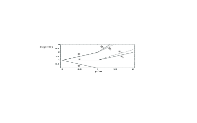
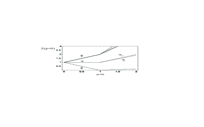
Figure 3: We present the Gaps ($E(p=0)$) for the polar phase (left panel) and the apolar (right panel) of the theory as function of the chemical potential in units of $m$. Left Panel: Before condensation each line describes three degenerate massive states. After condensation $\mu>m$ the dashed lines represent two states while the solid lines represent one state each except for the three gapless states. We used the following values for the plot: $\lambda=1$, $\lambda^{\prime}=0.33$. Right Panel: Before condensation each line describes three degenerate massive states. After condensation $\mu>m$ the dashed line represents two states ($\psi_{V}$) while the solid lines one physical state each except for the two gapless states. We used the following values for the plot: $\lambda=1$, $\lambda^{\prime}=-0.3$.

III.2 The Apolar Phase Dispersion Relations and Gaps

We also solved the physical constraint for the apolar case. In this case the analytical analysis of the physical constraints and of the dispersion relations is complicated by the fact that the vacuum is complex. Since the computations are instructive but technical we provided them in the last appendix and summarize here the results. In this phase we have three broken generators but only two gapless modes: a type I and a type II goldstone boson. Since the unbroken generator is a linear combination of a rotation and the generator for the internal $U(1)$ symmetry the gaps and the dispersion relations lose the straightforward and nice classification in doublets (i.e. vectors) and scalars with respect to a standard rotation. The gaps in this phase, and for a specific choice of the couplings, are displayed in the right panel of Fig. 3. Before condensation each line describes three degenerate massive states. After condensation $\mu>m$ the dashed line ($\psi_{V}$) represents two states while the solid lines one physical state each except for the two gapless states. We used the following values for the plot: $\lambda=1$, $\lambda^{\prime}=-0.3$. The dispersion relations too, in the $\delta=0$ limit, display a more complex structure which does not alter the gapless excitation structure and goldstone counting.

III.3 Breaking the $Z_{2}$ symmetry.

We now comment on what happens if we allow $Z_{2}$ symmetry breaking terms such as the $\delta$ term. Before including the chemical potential in the direction $T^{3}$ the absence of the $\delta$ term prevents an odd number of vectors to be present in any vertex of the theory. Since this term involves 3 fields it will not affect the dispersion relations before condensation. After condensation has taken place the vacuum structure (due to our ansatz) is also unaffected by this term. Since the goldstone states are the fluctuations around the vacuum in the direction of some of the continuously broken symmetries their general properties are also expected not to be disrupted. The $\delta$ term will, however, change some of the details of the dispersion relations. The possible quadratic terms in the fields emerging after condensation will always mix the $\psi$ state with a $\phi$ one and their effect will be investigated elsewhere.

IV Physical Applications and Conclusions

We investigated the phase structure of the relativistic massive vector condensation phenomenon due to a non zero chemical potential associated to some of the global conserved charges of the theory. The possible phase structure is very rich. Indeed according to the value assumed by $\lambda^{\prime}$ we have three independent phases. The polar phase with $\lambda^{\prime}$ positive is characterized by a real vacuum expectation value and 3 goldstone bosons of type I. The apolar phase for $\lambda^{\prime}$ negative has a complex vector vacuum expectation value spontaneously breaking CP. In this phase we have one goldstone boson of type I and one of type II while still breaking 3 continuous symmetries. The third phase has an enhanced potential type symmetry and 3 goldstone bosons one of type I and two of type II.

We also discovered that if we force the self interaction couplings $\lambda$ and $\lambda^{\prime}$ to be identical, as predicted in a Yang-Mills massive theory, our ansatz for the vacuum does not lead to a stable minimum when increasing the chemical potential above the mass of the vectors. A possible resolution of such an instability is that the chemical potential can be at most as large as the vector mass. This case it very similar to the Bose-Einstein condensation phenomenon for an ideal bose gas at high chemical potential. Interestingly the gauge coupling limit is often adopted in literature to economically describe, for example, the QCD composite vector field $\rho$. We hence suggest that lattice studies at high isospin chemical potential in the vector channel for QCD might be able to, indirectly, shed light on this sector of the theory at zero chemical potential. More generally the hope is that these studies might help understanding how to construct consistent theories of interacting massive higher spin fields not necessarily related to a gauge principle.

We also developed a formalism which enabled us to investigate the vacuum structure and dispersion relations in the spontaneously broken phase of the theory. Our results are helpful when trying to go beyond the classical and tree approximation. Our present studies are readily applicable to a number of physical phenomena of topical interest. For example in the framework of 2 color QCD at high baryon chemical potential vector condensation has been predicted in Lenaghan:2001sd ; Sannino:2001fd . Recent lattice studies Alles:2002st seem to support it. The present analysis while reinforcing the scenario of vector condensation shows that we can have many different types of condensations with very distinct signatures. Some details of other possible physical applications are presented in Sannino:2001fd . The present analysis can be straightforwardly extended to a general number of space dimensions Sannino:2001fd which may be useful for more exotic scenarios related to the phenomenon of vector condensation Li:2002iw .

Appendix A Lagrangian in cartesian components

It is helpful to know also the different terms of the theory in cartesian components. We start with the vector Lagrangian presented and studied in the main test:

$${\cal L} = -\frac{1}{4}F^{a}_{\mu\nu}F^{a{\mu\nu}}+\frac{m^{2}}{2}A_{\mu}^{a}A^{a\mu}+\delta\,\epsilon^{abc}\partial{\mu}A_{a\nu}A^{\mu}_{b}A^{\nu}_{c}-\frac{\lambda}{4}\left(A^{a}_{\mu}A^{a{\mu}}\right)^{2}+\frac{\lambda^{\prime}}{4}\left(A^{a}_{\mu}A^{a{\nu}}\right)^{2}\ ,$$ (81)

with $F_{\mu\nu}^{a}=\partial_{\mu}A^{a}_{\nu}-\partial_{\nu}A^{a}_{\mu}$, $a=1,2,3$ and metric convention $\eta^{\mu\nu}={\rm diag}(+,-,-,-)$. Here, $\delta$ is a real dimensionless coefficient, $m^{2}$ is the tree level mass term and $\lambda$ and $\lambda^{\prime}$ are positive dimensionless coefficients with $\lambda>\lambda^{\prime}$.

After including a nonzero chemical potential associated to a given conserved charge - related to the generator (say $B$) - in the the following way:

$$\partial_{\nu}A_{\rho}\rightarrow\partial_{\nu}A_{\rho}-i\left[B_{\nu}\ ,A_{\rho}\right]\ ,$$ (82)

with $B_{\nu}=\mu\,\delta_{\nu 0}B\equiv V_{\nu}B$ where $V=(\mu\ ,\vec{0})$. The vector kinetic term modifies according to:

$${\rm Tr}\left[F_{\rho\nu}F^{\rho\nu}\right] \rightarrow {\rm Tr}\left[F_{\rho\nu}F^{\rho\nu}\right]-4i{\rm Tr}\left[F_{\rho\nu}\left[B^{\rho},A^{\nu}\right]\right]-2{\rm Tr}\left[\left[B_{\rho},A_{\nu}\right]\left[B^{\rho},A^{\nu}\right]-\left[B_{\rho},A_{\nu}\right]\left[B^{\nu},A^{\rho}\right]\right]\ .$$ (83)

The terms induced by $F_{\mu\nu}F^{\mu\nu}$, after integration by parts, yields Lenaghan:2001sd

$${\cal L}_{kinetic} = \frac{1}{2}A_{\rho}^{a}\left\{\delta_{ab}\left[g^{\rho\nu}\Box-\partial^{\rho}\partial^{\nu}\right]-4i\gamma_{ab}\left[g^{\rho\nu}V\cdot\partial-\frac{V^{\rho}\partial^{\nu}+V^{\nu}\partial^{\rho}}{2}\right]+2\chi_{ab}\left[V\cdot Vg^{\rho\nu}-V^{\rho}V^{\nu}\right]\right\}A_{\nu}^{b}$$ (84)

with

$$\gamma_{ab}={\rm Tr}\left[T^{a}\left[B,T^{b}\right]\right]\ ,\qquad\chi_{ab}={\rm Tr}\left[\left[B,T^{a}\right]\left[B,T^{b}\right]\right]\ .$$ (85)

For $B=T^{3}$ we have

$$\gamma_{ab}=-\frac{i}{2}\epsilon^{ab3}\ ,\quad\chi_{11}=\chi_{22}=-\frac{1}{2}\ ,\quad\chi_{33}=0\ .$$ (86)

The chemical potential induces a “magnetic-type” mass term for the vectors at tree-level.

The trilinear term with a single derivative is:

$${\cal L}_{\delta}=\delta\,\epsilon^{abc}\partial_{\mu}A_{a\nu}A^{\mu}_{b}A^{\nu}_{c}+\delta\,\left(V\cdot A^{b}\right)A^{a\nu}A_{\nu}^{c}\left[\delta^{3b}\delta^{ac}-\delta^{3c}\delta^{ab}\right]\ .$$ (87)

.

Appendix B Cylindrical Coordinates

Here we summarize all of the terms in the Lagrangian using the cylindrical coordinates:

$$\phi_{\mu} = {1\over\sqrt{2}}(A^{1}_{\mu}+iA^{2}_{\mu})\ ,\qquad\phi^{\ast}_{\mu}={1\over\sqrt{2}}(A^{1}_{\mu}-iA^{2}_{\mu})\ ,\qquad\psi_{\mu}=A^{3}_{\mu}\ ,$$ (88)

The quadratic, cubic and quartic terms - in the vector fields - now reads:

$${\cal{L}}_{\rm quadratic} = {1\over 2}\,\psi^{\mu}\,[g_{\mu\nu}[\partial^{2}+m^{2}]-\partial_{\mu}\partial_{\nu}]\,\psi^{\nu}+\left\{{1\over 2}\,{\phi^{\ast}}^{\mu}\,\left(g_{\mu\nu}[D^{2}+m^{2}]-D_{\mu}D_{\nu}\right)\,\phi^{\nu}+c.c.\right\}$$ (89)

$${\cal L}_{cubic} = -i\,\delta\partial_{\mu}\psi_{\nu}\left({\phi^{\ast}}^{\mu}\cdot\phi^{\nu}\right)-i\,\delta\psi^{\nu}\left(\partial_{\mu}\phi^{\ast}_{\nu}\phi^{\mu}\right)-i\,\delta\psi^{\mu}\left(\partial_{\mu}\phi^{\ast}_{\nu}\phi^{\nu}\right)+{\rm c.c.}$$ (90)

$$-2\delta\,V\cdot\psi\left(\phi^{\ast}\cdot\phi\right)-\delta\,\left[V\cdot\phi^{\ast}\left(\phi\cdot\psi\right)+{\rm c.c.}\right]\ .$$

$${\cal L}_{4-vectors}=-\frac{\lambda}{4}\left(A^{a}_{\mu}A^{a{\mu}}\right)^{2}+\frac{\lambda^{\prime}}{4}\left(A^{a}_{\mu}A^{a{\nu}}\right)^{2} = {\lambda^{\prime}-2\lambda\over 2}(\phi^{\ast}\cdot\phi)^{2}+{\lambda^{\prime}\over 2}|(\phi\cdot\phi)|^{2}+{\lambda^{\prime}-\lambda\over 4}(\psi\cdot\psi)^{2}$$

$$-{\lambda}(\phi^{\ast}\cdot\phi)(\psi\cdot\psi)+\lambda^{\prime}|(\psi\cdot\phi)|^{2}$$

Appendix C Dispersion relations for the apolar phase

In this case the vev is proportional to the vector:

$$n^{\mu}=\frac{1}{\sqrt{2}}\left(\begin{array}[]{c}0\\ 1\\ \imath\\ 0\\ \end{array}\right)\ ,\quad{\rm with}\quad n^{2}={n^{\ast}}^{2}=0\ ,\quad{\rm and}\quad n\cdot n^{\ast}=-1\ .$$ (97)

The quadratic Lagrangian term for the field $\psi$ takes the form:

$${1\over 2}\,\psi^{\mu}\,[g_{\mu\nu}[\partial^{2}+\bar{m}^{2}]-\partial_{\mu}\partial_{\nu}]\,\psi^{\nu}+\frac{{\kappa}}{2}\psi^{\mu}\left(n_{\mu}n_{\nu}^{\ast}+n_{\mu}^{\ast}n_{\nu}\right)\psi^{\nu}\ ,$$ (98)

and the constraint equation reads:

$$\bar{m}^{2}\partial\cdot\psi=-{\kappa}\left[n\cdot\partial\left(n^{\ast}\cdot\psi\right)+n^{\ast}\cdot\partial\left(n\cdot\psi\right)\right]\ .$$ (99)

We define the following projectors

$${\cal P}_{\mu\nu}=g_{\mu\nu}-{\cal L}_{\mu\nu}\ ,\qquad{\cal L}_{\mu\nu}=\frac{n_{\mu}n^{\ast}_{\nu}+n_{\nu}n^{\ast}_{\mu}}{n\cdot n^{\ast}}\ .$$ (100)

Now ${\cal L}_{\mu\nu}$ has two non zero components (i.e. $\mu=\nu=x$ and $\mu=\nu=y$) and hence projects out two real scalars while ${\cal P}_{\mu\nu}$ has non zero the temporal and the zed component projecting out a vector which lives in $1+1$ dimensions (i.e. again a scalar field). It is convenient to split $\psi$ as follows:

$$\psi_{\mu}={\psi_{S}}_{\mu}+\frac{n_{\mu}}{n\cdot n^{\ast}}{\psi_{D}}+\frac{n_{\mu}^{\ast}}{n\cdot n^{\ast}}{\psi_{D}^{\ast}}\ ,\qquad{{\psi}_{D}}=n^{\ast}\cdot\psi\ ,$$ (101)

Using these fields plus the constraint the Lagrangian becomes:

$${\cal L} = \frac{1}{2}{\psi_{S}}_{\mu}\left(\partial^{2}+\bar{m}^{2}\right){\psi_{S}}^{\mu}-\psi_{D}^{\ast}\left(\partial^{2}+\widetilde{m}^{2}+\frac{\kappa^{2}}{\bar{m}^{4}}(n\cdot\partial)(n^{\ast}\cdot\partial)\right){\psi_{D}}$$ (102)

$$-\frac{\kappa^{2}}{2\bar{m}^{4}}\left[{\psi_{D}}(n\cdot\partial)^{2}{\psi_{D}}+\psi_{D}^{\ast}(n^{\ast}\cdot\partial)^{2}\psi_{D}^{\ast}\right]\ ,$$

with

$$\Delta^{2}_{\psi_{D}}\equiv\widetilde{m}^{2}=\bar{m}^{2}-\kappa\ ,\qquad\Delta^{2}_{\psi_{S}}\equiv\bar{m}^{2}\ .$$ (103)

Diagonalizing the $D$ and $S$ sector independently we deduce the following dispersion relations:

$$E_{{\psi_{D}}^{1}}^{2} = \Delta^{2}_{\psi_{D}}+{\bf p}^{2}\ ,\qquad E_{{\psi_{D}}^{2}}^{2}=\Delta^{2}_{\psi_{D}}+v^{2}_{D^{2}}\left(p^{2}_{x}+p^{2}_{y}\right)+p^{2}_{z}\ ,\qquad E_{\psi_{S}}^{2}=\bar{m}^{2}+{\bf p}^{2}\ ,$$ (104)

with

$$v^{2}_{D^{2}}=1-\frac{\kappa^{2}}{\bar{m}^{4}}\ .$$ (105)

Substituting for the vev:

$$\Delta^{2}_{\psi_{S}}=\bar{m}^{2}=\mu^{2}+\frac{\lambda^{\prime}}{2\lambda-\lambda^{\prime}}\left(\mu^{2}-m^{2}\right)\ ,\quad\kappa=\frac{\lambda^{\prime}}{2\lambda-\lambda^{\prime}}\left(\mu^{2}-m^{2}\right)\ ,\quad\Delta^{2}_{\psi_{D}}=\mu^{2}\ .$$ (106)

We see that in the $\psi$ sector of the theory when $\delta$ is zero two states have isotropic dispersion relations but are not degenerate. The two degenerate states have different momentum dependence.

C.1 The $\phi$ dispersion relations

The general quadratic Lagrangian in a 2 component formalism and in the presence of the complex vev for $\phi$ reads:

$$\frac{1}{2}{\chi^{\dagger}}^{\mu}\left[g_{\mu\nu}\left(\Delta^{2}+\overline{M}\right)-\Delta_{\mu}\Delta_{\nu}\right]\chi^{\nu}+\frac{1}{2}{\chi^{\dagger}}^{\mu}{\cal K}_{\mu\nu}\chi^{\nu}\ .$$ (107)

with

$$\overline{M}=\left(\begin{array}[]{cc}\mu^{2}&0\\ 0&\mu^{2}\\ \end{array}\right)\ ,\quad{\cal K}_{\mu\nu}=(m^{2}-\mu^{2})\left(\begin{array}[]{cc}n_{\mu}n^{\ast}_{\nu}-\gamma\,n^{\ast}_{\mu}n_{\nu}&n_{\mu}n_{\nu}\\ n^{\ast}_{\mu}n^{\ast}_{\nu}&n^{\ast}_{\mu}n_{\nu}-\gamma\,n_{\mu}n^{\ast}_{\nu}\\ \end{array}\right)\ ,\quad{\gamma}=\frac{2\lambda^{\prime}}{2\lambda-\lambda^{\prime}}\ .$$ (112)

Note that the matrix ${\cal K}_{\mu\nu}$ Lorentz structure is solely determined by the vector vev. The quadratic equation of motion leads to the following physical constraint:

$$\overline{M}\Delta_{\nu}\chi^{\nu}=-\Delta^{\mu}{\cal K}_{\mu\nu}\chi^{\nu}.$$ (113)

We split $\chi$ as follows:

$$\chi_{\mu}={\Phi_{S}}_{\mu}+\frac{n_{\mu}}{n\cdot n^{\ast}}{\widetilde{\Phi}_{D}}+\frac{n_{\mu}^{\ast}}{n\cdot n^{\ast}}{\Phi_{D}}\ ,\qquad{{\widetilde{\Phi}}_{D}}=n^{\ast}\cdot\chi\ ,\quad{\Phi_{D}}=n\cdot\chi\ .$$ (114)

Now $\Phi_{S}$, $\Phi_{D}$ and $\widetilde{\Phi}_{D}$ represent three independent (2-components) physical states. (i.e. using these fields plus the constraint the quadratic term Lagrangian can be compactly written as:

$$\frac{1}{2}{{\Phi}_{S}^{\mu}}^{\dagger}\left(\Delta^{2}+\overline{M}\right){{\Phi}_{S}}_{\mu}-\frac{1}{2}{{{\cal T}}_{D}}^{\dagger}\left[\left(\Delta^{2}+\overline{M}\right)\times{\bf 1}+\frac{U}{\mu^{4}}-Q\right]{\cal T}_{D}\ ,$$ (115)

with

$${\cal T}_{D}=\left(\begin{array}[]{c}\widetilde{\Phi}_{D}\\ \Phi_{D}\\ \end{array}\right)\ ,\quad U=\left(\begin{array}[]{cc}{n^{\ast}}{\cal K}^{\dagger}\partial\,\partial{\cal K}{n}&{n^{\ast}}{\cal K}^{\dagger}\partial\,\partial{\cal K}{n^{\ast}}\\ n{\cal K}^{\dagger}\partial\,\partial{\cal K}{n}&n{\cal K}^{\dagger}\partial\,\partial{\cal K}{n^{\ast}}\\ \end{array}\right)\ ,\quad Q=\left(\begin{array}[]{cc}n^{\ast}{\cal K}n&n^{\ast}{\cal K}n^{\ast}\\ n{\cal K}n&n{\cal K}n^{\ast}\\ \end{array}\right)$$ (122)

where ${\cal T}_{D}$ is a 4 column vector, $U$ and $Q$ are four-dimensional matrices. $n{\cal K}^{\dagger}\partial\equiv n^{\mu}{\cal K}^{\dagger}_{\mu\nu}\partial^{\nu}$ is a two dimensional matrix.

The dispersion relations in the $S$ sector are now straightforward and we deduce the following two states:

$$E_{GB-II} = \frac{p^{2}}{2\mu^{2}}+{\cal O}(p^{4})\ ,$$ (123)

$$E_{WBGB} = 2\mu^{2}+\frac{p^{2}}{2\mu^{2}}+{\cal O}(p^{4})\ .$$ (124)

The first state is a type II goldstone boson while the second state is the would be goldstone boson e.g. the one which would have been massless if we had no breaking of the Lorentz symmetry. For the D sector the diagonalization can be performed analytically when setting the momentum in the $x$ and $y$ direction to zero and we get:

$$E_{GB-I}^{2} = {v_{z}}^{2}\,p_{z}^{2}+{\cal O}(p^{4})\ ,$$ (125)

$$E_{\Phi_{A}}^{2} = 2(3\mu^{2}-m^{2})+(2+v_{z}^{2})\,p_{z}^{2}+{\cal O}(p^{4})\ ,$$ (126)

$$E_{\Phi_{B}}^{2} = \Delta^{2}_{\Phi_{B}}+v^{2}_{\Phi_{B}}\,p_{z}^{2}+{\cal O}(p^{4})\ ,$$ (127)

$$E_{\Phi_{C}}^{2} = \Delta^{2}_{\Phi_{C}}+v^{2}_{\Phi_{C}}\,{p_{z}^{2}}+{\cal O}(p^{4})\ .$$ (128)

This sector of the theory contains a goldstone boson of type I and 3 massive states.

In the following we summarize the nine physical gaps related to this phase:

$$\begin{array}[]{|cll||c|}\hline\cr&&&\\ \Delta^{2}_{GLess}&=&0\ ,&{\rm 2~{}States}\\ &&&\\ \Delta^{2}_{\phi_{WBGB}}&=&4\mu^{2}&{\rm 1~{}State}\\ &&&\\ \hline\cr&&&\\ \Delta^{2}_{\phi_{A}}&=&2\,(3\mu^{2}-m^{2})&{\rm 1~{}State}\\ &&&\\ \Delta^{2}_{\phi_{B}}&=&\frac{2}{(2\lambda-\lambda^{\prime})^{2}}(h1+\sqrt{h2})&{\rm 1~{}State}\\ &&&\\ \Delta^{2}_{\phi_{C}}&=&\frac{2}{(2\lambda-\lambda^{\prime})^{2}}(h1-\sqrt{h2})&{\rm 1~{}State}\\ \hline\cr\end{array}$$ (140)

$$\begin{array}[]{|cll||c|}\hline\cr&&&\\ \Delta^{2}_{\psi_{V}}&=&\mu^{2}&{\rm 2~{}States}\\ &&&\\ \Delta^{2}_{\psi_{S}}&=&\mu^{2}+\frac{\lambda^{\prime}}{2\lambda-\lambda^{\prime}}(\mu^{2}-m^{2})&{\rm 1~{}State}\\ \hline\cr\end{array}$$ (145)

with:

$$h1=m^{2}(2\lambda-\lambda^{\prime})\lambda^{\prime}+4\lambda^{2}\mu^{2}-6\lambda\lambda^{\prime}\mu^{2}+2{\lambda^{\prime}}^{2}\mu^{2},\qquad h2=\mu^{2}\,(2\lambda-\lambda^{\prime})^{3}\,(2m^{2}\lambda^{\prime}+(2\lambda-3\lambda^{\prime})\mu^{2})\ .$$ (146)

References

(1)
A. D. Linde,
Phys. Lett. B 86, 39 (1979).
(2)
J. Ambjorn and P. Olesen,
Phys. Lett. B 218, 67 (1989) [Erratum-ibid. B 220,
659 (1989)], ibid. B 257, 201 (1991), Nucl. Phys. B 330, 193 (1990).
(3)
N. S. Manton,
Nucl. Phys. B 158, 141 (1979).
(4)
Y. Hosotani,
Annals Phys. 190, 233 (1989).
(5)
L. F. Li,
arXiv:hep-ph/0210063.
(6)
G. E. Brown and M. Rho,
Phys. Rev. Lett. 66, 2720 (1991).
(7)
M. Harada and K. Yamawaki,
Phys. Rev. Lett. 86, 757 (2001) [arXiv:hep-ph/0010207].
(8) M. Bando, T. Kugo and K. Yamawaki, Phys. Rept. 164, 217
(1988).
(9)
R. D. Pisarski and D. H. Rischke,
Phys. Rev. D 61, 074017 (2000) [arXiv:nucl-th/9910056].
(10)
M. Buballa, J. Hosek and M. Oertel,
arXiv:hep-ph/0204275.
(11)
J. T. Lenaghan, F. Sannino and K. Splittorff,
Phys. Rev. D 65, 054002 (2002) [arXiv:hep-ph/0107099].
(12)
F. Sannino and W. Schafer,
Phys. Lett. B 527, 142 (2002) [arXiv:hep-ph/0111098].
(13)
B. Alles, M. D’Elia, M. P. Lombardo and M. Pepe,
arXiv:hep-lat/0210039. (See references therein for 2 color QCD at
high baryon chemical potential)
(14)
S. Muroya, A. Nakamura and C. Nonaka,
arXiv:hep-lat/0211010.
(15)
D.M. Stamper-Kurn, M.R. Andrews, A.P. Chikkatur, S. Inouye,
H.-J. Miesner, J. Stenger, and W. Ketterle, Phys. Rev. Lett. 80, 2027 (1998).
(16)
G. Volovik,
J. Low. Temp. Phys. 121, 357 (2000)
[arXiv:cond-mat/0005431] and references therein; U. Leonhardt and
G. E. Volovik,
JETP Lett. 72, 46 (2000) [arXiv:cond-mat/0003428].
(17)
H.B. Nielsen and S. Chadha,
Nucl. Phys. B105, 445 (1976).
(18)
T. Schafer, D. T. Son, M. A. Stephanov, D. Toublan and
J. J. Verbaarschot,
hep-ph/0108210.
V. A. Miransky and I. A. Shovkovy,
hep-ph/0108178.
(19) Ö. Kaymakcalan, S. Rajeev and J. Schechter,
Phys. Rev. D30, 594 (1984); J. Schechter, Phys. Rev. D34, 868 (1986); P. Jain, R. Johnson, Ulf-G. Meissner, N. W. Park
and J. Schechter, Phys. Rev. D37, 3252 (1988).
(20) Ö. Kaymakcalan and J. Schechter, Phys. Rev. D31,
1109 (1985).
(21) T. Appelquist, P.S. Rodrigues da Silva and F. Sannino,
Phys. Rev. D60, 116007 (1999), hep-ph/9906555.
(22) Z. Duan, P.S. Rodrigues da Silva and F. Sannino, Nucl. Phys. B 592, 371
(2001), hep-ph/0001303.
(23)
G. Ecker, J. Kambor and D. Wyler,
Nucl. Phys. B 394, 101 (1993).
(24)
J. I. Kapusta, Finite-temperature field theory, Cambridge
Monographs on Mathematical Physics (1993).